Embed Size (px)
Citation preview
1
Stochastic Frontier Analysis of Biological Agents (Microbial Inoculants) Input
Usage in Apple Production
Holcer Chavez1, Denis Nadolnyak1 and Joseph Kloepper2
1Department of Agricultural Economics & Rural Sociology, Auburn University, Auburn Alabama 2Department of Entomology and Plant Pathology, Auburn University, Auburn Alabama
Selected Paper prepared for presentation at the Southern Agricultural Economics Association Annual Meeting, Birmingham, AL, February 4-7, 2012
Copyright 2012 by H. Chavez, D. Nadolnyak and J. Kloepper. All rights reserved. Readers may make verbatim copies of this document for non-commercial purposes by any means, provided that this copyright notice appears on all such copies.

2
Abstract
This paper analyzes the effect of Microbial Inoculants (MI) Technology over pesticide and yields
in apples using 2007 farm data. The results show that pesticide usage is not reduced by MI
applications; however, there is a significant positive effect over the outputs. Farmers’ efficiency
rates are on average 37%.
Introduction
Currently, disease management in crops worldwide is heavily dependent upon application of
synthetic (chemical) pesticides for pathogen and insect control. However, the excess application
of pesticides can enhance the development of pest resistance, thus requiring more chemicals or
increasing the damage of pests. Also, stricter regulations compromising yields for environmental
objectives discourage the use of pesticides. As an example, regulations in the United States are
based almost entirely on the direct effects on health and environment (White, 1998). Moreover,
chemical pesticides’ prices have been increasing as fuel prices have been increasing and because
big portion of the market power is shared only by few big transnational producers who are
becoming the only suppliers (Marcoux and Urpelainen, 2011; Fernandez-Cornejo and Just,
2007). All of this works against farmer’s profit maximizing objectives and makes them to look
for alternatives that can keep up with higher yields.
In the last years, global demand for more environmentally friendly products and sustainable
production systems has been increasing. In this context, biological control products offer an
attractive alternative to synthetic pesticides. According to Pal and Gardener (2006) “Biological
control refers to the purposeful utilization of introduced or resident living organisms, other than

3
disease resistant host plants, to suppress the activities and populations of one or more plant
pathogens”
Over the last two decades, biological control of plant pathogens has emerged as a viable disease
control strategy (Harman et al., 2010; Singh et al., 2011). Microbial inoculants (MI) is a type of
biocontrol agent that includes bacteria and fungi, representing an environmental friendly
approach to reduce losses due to pest and diseases or showing as an alternative to chemical
pesticides (Lugtenberg et al., 2002). Impact assessments of biological control are measured by
cost-benefit analysis in an ex-ante situation but, for ex-post analysis, a production function, that
can have an integrated damage control, is a standard procedure in agricultural production
economics. The chosen crop is apples as there are already some products being applied and
because according to the United States-based Environmental Working Group (EWG), apples
rank as the most contaminated fruit and vegetable produce (Lloyd, 2011; Bagnato, 2011)
The objectives of this study are to quantify the contribution of MI and other production factors to
the 2007 U.S. apples yields, and to estimate the effects of MI usage over pesticide usage.
Data basis
USDA’s 2007 Agricultural Resource Management Survey (ARMS) data on apple production
was used for this study. This survey contains information on the, production practices, inputs and
costs, and financial performance of America’s farm households. Most of the data come from the
Phase 2 part of the survey. Only conventional (non organic) farmers were considered as intend
was estimate the complementary and/or supplemental effect over pesticides. Under the “pest
management practices” section of the production practices and costs reports (phase 2) of the
survey, an item referring to biological control was used as the variable of interest. In the sample
4
of 547 conventional farms, 197 farms were using one or more biological control products, from
which the main ingredient included one of the following: Granulovirus, Bacillus thuringensis,
Bacillus subtilis, Bacillus pumilus and Thricoderma sp. Figure 1 shows the percentage
represented by each biological agent, from which, 67% fall into the MI definition.
[Place Figure 1 Approximately Here]
MI provides good resistance to different varieties of insects and diseases for apples compared to
others biological agents used in this study. For example, the Granulovirus is only used against
Codling moth (Cydia pomonella), but Bacillus thuringensis has been proved to work against
Codling moth, Apple pandemis, Leafrollers, Western tussock moth, Velvetbean caterpillar and
Green fruitworm (California, 1999). Bacillus subtilis has been proven to work against Fire
Blight, Botrytis, Sour Rot, Rust, Sclerotinia, Powdery Mildew, Bacterial Spot and White Mold
(Peighamy-Ashnaei et al., 2008; Sundin et al., 2009). However, there are many other pest and
diseases to which MI agents do not provide resistance; Therefore, MI does not completely
eliminate the need to use chemical pesticides. For easiness of the study, from now on MI will
refer to all biological agents used in the data (as Granulovirus was often combined with an MI
agent).
Seven states were represented in the survey: Michigan, Oregon, New York, Pennsylvania, North
Carolina, California and Washington, the last one used as the base. Washington was used as the
base for its continuous and successful history of apple production.
Data analysis and framework
Effects of MI on pesticide application

5
As a first step, the summary statistics of those farmers using and not using the technology are
compared to have a quick look of what might have been happening. The variable pesticide is
only including insecticide and fungicide applications, herbicides were not took into account as
they fall into other category. In order to confirm the findings, a more precise quantification was
needed. A Cobb-Douglas type functional form was estimated using OLS regression to estimate
the technology’s effect over the pesticide use. This was calculated using plot and farmer
characteristic. The amount of pesticide (pest) in pounds per acre can be expressed as:
Log (Pest) = Log (A) + ∑ βi Log (X) + ∑ βi Log (VS) + β1 (MI) + ∑ β2 (K) + ε (1)
Where A is the intercept, X is a vector of direct production inputs, VS is the value of sales per
acre. In this study, value of sales per acre is used as a proxy for yields per acre. With cross-
sectional data, using a nominal output measure (revenue) or a physical production output
measure makes very little difference as it was stated by Mairesse and Jaumandreu (2005). MI is a
dummy variable which takes the value of one for MI plots and zero otherwise1. Lastly, K is a
vector of other determining factors such as experience, expenditure on pesticide over pesticide
(as proxy of price), pest pressure and a state area variable (dummy) as proxy for the different
agro climate conditions found in these areas.
Productivity and damage control
A production function or frontier is defined as the specification, given an available technology,
of the maximum amount of output possible to produce given a certain quantity of inputs and
combinations. It measures the effect of each exogenous variable over the quantity produced.
1 It would have been advantageous to use a quantitative measure of the MI applications but the AMRS survey data, the most comprehensive data available to us, only contains a categorical measure of MI use.

6
Different types of production functions are estimated to measure MI impact over the output
production. First, a Cobb-Douglas specification is used, which in general is the standard
approach for a production function. We estimate the following relationship:
Log (VS) = Log (A) + ∑ βi Log (X) + β1 (MI) + ∑ βi (P) + ε (2)
Where VS is the value of sales per acre, A is the intercept, X is a vector of direct production
inputs, MI is the microbial inoculants dummy variable and P is a vector of experience and area
variables.
In agricultural production, inputs can be divided into 2 main categories: standard factors of
production (e.g. land, labor, capital, etc.) and damage control agents (e.g. pesticides, herbicides,
and biological control). The damage control agents enhance productivity indirectly by preventing
output loses. Thus, a damage control function needs to be integrated in a production function as
inputs cannot be treated in the same way. In the analysis of pesticide productivity, the use of a
standard Cobb-Douglas function is criticized for treating pesticide as a yield increasing
production factor and not capturing knowledge about physical and biological processes of pest
control agents. Lichtenberg and Zilberman (1986) explain that using a Cobb-Douglas functional
form results in overestimation of productivity of damage control inputs, while productivity of
other factors will be underestimated. To address this problem they introduce the concept of
damage control functions. They propose using a separate damage control function G, which is
linked to the production function in a multiplicative way.
Y = f (X) g (Z) (3)
Where X denotes normal inputs, and Z pest control agents. g (Z) possesses the properties of a
cumulative distribution function, with values defined in the (0, 1) interval. Thus, f(X) is the
potential maximum yield to be obtained with zero pest damage or maximum pest control.

7
For f (·) we use the same Cobb-Douglas functional form as before, whereas for g (·) different
functional forms can be assumed and specification can be crucial for the parameter estimation
results (Carrasco-Tauber and Moffitt, 1992; Fox and Weersink, 1995). But, since up until now
there is no consensus on which specification best suits the purpose, a logistic specification is
used as it generally represents the pest abatement relationship quite well and it was used in the
study made by Qaim and De Janvry (2005).
g (Z) = [1 + exp (μ - α1Pest – α2MI)]-1 (4)
Log (VS) = Log (A) + ∑ βi Log (x) + ∑ βi (P) + Log (g (Z)) + ε (5)
The parameter μ is interpreted as the fixed damage effect. A standard Cobb-Douglas production
function treating pesticide and biological control as conventional production factors is also
estimated for comparison purposes.
A problem in estimating production functions is that pest variables tend to be correlated with the
production function error term ε. This is because unobserved factors like climate conditions can
result in both high input levels of insecticides and low yields (Huang et al., 2002) and also
because insecticides applied to high responses of pest pressure can become a problem
(Widawsky and et al., 1998).To address this problem, a two-stage least square (2SLS) estimation
is used and the pesticide variable is instrumented. The instrumental variable (IV) has to have the
following characteristics: cov (IV, ε) =0 as it should not be correlated with the error term, and
cov (IV, pest) ≠0 and highly correlated. For the IV we will use the amount of active ingredient.
Furthermore, production functions and pesticide use function are tested for multicollinearity and
corrected for heteroskedasticity, two other potential problems with cross-sectional data.
8
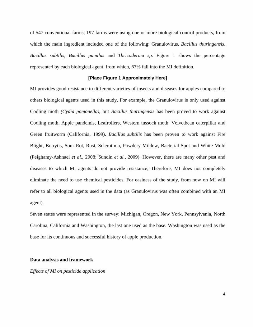
Stochastic production frontier
In addition, to the 2 previous Cobb-Douglas models, a Stochastic Production Frontier (SPF) is
estimated. In contrast to a regular production function, SPF allows for inefficiency as it does not
assume that all farmers are producing on the production possibilities frontier.
The SPF estimates a frontier function that can be interpreted as the technological constraint for
each farming system. How far from the frontier the farm operation is located addresses the
farm’s performance or technical efficiency. Traditional regression approaches, such as ordinary
least squares (OLS), can be used to estimate parameters of production, cost, and/or profit
functions; however, the estimates only reflect the average farm performance.
The stochastic frontier model considers random shocks on the production process. Assume that
cross sectional data for the quantities of N inputs used to produce a single output are available to
I producers. A SPF model is written as
Yi = f (Xi; β) exp {𝑣�} 𝑇𝐸� (6)
Where Yi is the scalar output of producer i, i = 1, . . . , I, Xi is a vector of N inputs used by
producer i, f (Xi; β) is the deterministic production frontier, β is a vector of technology
parameters to be estimated, exp {𝑣�} captures the effects of statistical noise, and TEi is the output
oriented technical efficiency of producer i. [f (Xi; β) · exp {𝑣�}] is the SPF. It consists of two
parts: a deterministic component f (Xi; β) common to all producers and a producer-specific
component exp {𝑣�} which captures the effect of random shocks on each producer.
Now equation (6) can be rewritten as
𝑇𝐸� = ���(��;�).���{��}
(7)

9
Which defines technical efficiency as the ratio of observed output to the maximum feasible
output in an environment characterized by exp {𝑣�}. It follows that 𝑌� achieves its maximum
feasible value of [f (Xi; β) · exp {𝑣�}] if and only if 𝑇𝐸� = 1. Otherwise 𝑇𝐸� < 1 provides a
measure of the shortfall of observed output from maximum feasible output in an environment
characterized by exp {𝑣�}, which is allowed to vary across producers. Rewrite equation (7) as
𝑌� = f (Xi; β) exp {𝑣�} exp {−𝑢�} (8)
Where 𝑇𝐸� = exp {−𝑢�}. This form is chosen due to the simplification when taking natural
logarithms. Because we require that 𝑇𝐸�≤ 1, we have 𝑢� ≥ 0. Next, assume that f (Xi; β) is of the
log-linear Cobb- Douglas form. Alternative functional specifications are conceivable but this
specification is computationally convenient. The SPF model (8) becomes
Log 𝑌� = β0 + ∑ 𝛽� Log 𝑋��+ 𝑣� - 𝑢� (9)
Where 𝑣� is the two sided individual “noise” component, and 𝑢� is the nonnegative technical
inefficiency component of the error term. The distributional assumptions are (i) 𝑣� ∼ i.i.d. N (0,
𝜎�� ); (ii) 𝑢� ∼ i.i.d. N+ (0, 𝜎�� ), that is, as nonnegative half normal; and (iii) 𝑣� and 𝑢� are
distributed independently of each other and of the exogenous variables (Kumbhakar and Lovell,
2000). However, this Normal - Half Normal model implicitly assumes that the “likelihood” of
inefficient behavior monotonically decreases for increasing levels of inefficiency. In order to
generalize the model, allows u to follow a truncated normal distribution: (ii)’ 𝑢� ∼ i.i.d. N+ (μ,
𝜎��), where μ is the mode of the normal distribution and is truncated below at zero. The
Normal–Truncated Normal model, which has the three distributional assumptions (i), (ii)’, and
(iii), provides a somewhat more flexible representation of the pattern of efficiency in the data
(Kumbhakar and Lovell, 2000; Coelli et al., 2005).

10
The density function of v is
𝑓(𝑣) = ������
. exp{− ��
����} (10)
The truncated normal density function for u ≥ 0 is given by
𝑓(𝑣) = �
������(� ��� . exp{− (���)�
����} (11)
Where Φ (·) is the standard normal cumulative distribution function. When μ = 0, the density
function in equation (6) collapses to the half normal density function for the Normal–Half
Normal model. Point estimates for technical efficiency of each producer can be obtained by
means of
𝑇𝐸� = E [exp {−𝑢� } |𝜀� ] (12)
Where 𝜀� = 𝑣� −𝑢� .
Results and discussion
Pesticide use function
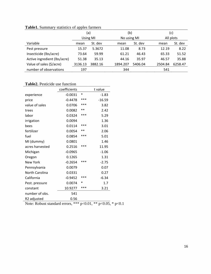
Patterns of pesticide use with and without MI are shown in column (a) and column (b)
respectively in Table 1. Heterogeneity was found to be characteristic of the sample but because
of the limited amount of observations, the sample was not subdivided.
[Place Table 1 Approximately Here]
Unexpectedly, and in contrast of with what was found previously regarding biological control by
Qaim and De Janvry (2003), the amount of pesticide used in plots also using MI is greater than
in those who are not using it. A comparison between columns (a) and (b) shows that there is a
20% increase in pesticide use associated with MI use but is only 14% if we refer to pesticide

11
active ingredient. However, this positive relationship could be explained by looking at some of
the other variables as pest pressure and value of sales are 38% and 65% greater respectively on
the plots using MI. It can be inferred then that farmers using MI have a bigger income and also
bigger pest problems and use more pest products (biological or not). So, there is a mixed effect
of costs increments (through the pesticide increase) and productivity gains.
The pesticide use function is estimated by an OLS Regression. Multicollineality detection was
performed through a Variance Inflation Factor (VIF), being the average of 1.48 and never larger
than 2.5 so it was not an issue. Robust standard errors were used to address heteroskedasticity
concerns.
[Place Table 2 Approximately Here]
All coefficients of the insecticide use function (pest) show the expected signs. As it was showed
in the summary statistics, MI, which in theory is supposed to be a substitute for pesticide, have a
positive coefficient but is not significant. This positive coefficient goes against previous studies
made in other crops like Cabbage (Jankowski et al., 2007) and cotton (Qaim and de Janvry,
2005; Huang et al., 2002). Nevertheless, the study made by Pemsl (2005) in cotton in china also
had a positive coefficient, but as in our study, it was not significant. This results can fit some
paradigms established about biocontrol like “the more a grower is willing to gamble the better
prospect he is to accept the idea of biological control. Those growers who cannot afford to lose
much (monetarily) usually do not want to risk using BC. They rather pay the price of
"prevention" insecticide treatments than take a chance on BC not coming through for them. The
prevention treatments are basically an insurance policy” (Peshin and Dhawan, 2009). Going back
to the results, for 1 extra year of experience, farmers use 0.31% less pesticide. The price
elasticity of pesticide use is -0.45%, i.e., if the pesticide price increases, by 1%, the amount of

12
pesticide used is reduced by 0.45%, which likely confirms our “insurance” argument. The
elasticity of pesticide use with respect to yield is 0.07 (for a 1% increase in yields, pesticide used
is increased by 0.07%) suggesting that pesticides only marginally increase yields and perhaps
mostly in the lower range. In the direct input category, for a 1% increase in trees, labor, bees,
fertilizer and fuel, the pesticide use increases by 0.0082%, 0.032%, 0.011%, 0.0054%, and
0.09% respectively. This could be due to higher general production intensity or more indirectly
as higher production inputs lead to higher yields and hence trigger higher insecticide use.
An interesting finding is that pesticide use increases with planted acres (production volume).
Only the states of California and New York are significantly compared to Washington (the base).
Pest pressure is a vector describing the degree of pest pressure exante (before spraying
decisions). In this study it was found to be positive significant (as usually is expected), meaning
that as pressure becomes worst there is an increase in pesticide use.
Production functions and frontier
As it can be seen in table 1, MI is positively correlated with the quantity of pesticides used, but
also increases yields to a significant extent. The net yield effect can be estimated econometrically
by using a production function approach. The first column in Table3 shows the results for the
production function considering all inputs as equal. As it was explained before, multicollinearity
and heteroskedasticity issues were tested and corrected. In addition, a Chow test was performed
in order to see if the two groups of farmers could be pooled together. Also, the problem of
endogeneity was addressed through a two stages least squares (2SLS) regression.
[Place Table 3 Approximately Here]

13
Microbial inoculatnts have a positive effect on output at the 10 % confidence level. All other
parameters remaining equal (ceteris paribus), MI increases apples yields by 21.25% per hectare,
which keeps up with what was speculated previously looking at the summary statistics. This also
corroborates the results found by Qaim and De Janvry (2003) where they found that the use of Bt
cotton increases yields by 507 kg./ha. in Argentina.
Insecticides also contribute substantially to higher yields. For a 1% increase in the amount of
pesticides used, the yield increased by 19%. Labor has a positive effect on apples output. For a 1
% increase in labor, the expected output increases by 0.05%. The impact of fertilizers is also
positive, but not statistically significant. The positive and significant coefficient at the harvested
acres suggests economies of size in the production of apples.
With respects to the area dummies, all the states have negative significant coefficients except for
California and Oregon. This means that, compared to the state of Washington, they produce less.
The coefficients of the production function with integrated damage control are very similar to
those in the standard production model but in this case our variable of interest is no significant.
MI has a t-value of 1.41 which is close to the minimum value to be significant. This can be due
to the fact that we chose a logistic damage control function. Without any pest control inputs, crop
damage would have been around 74%. As it was stated in the theory, it can be seen that
parameters of pesticide use was overestimated at 0.19 as compared to 0.002 An interesting fact is
that with the fixed damage effect of 74% and the marginal amount of damage contained by the
pesticide of only 0.002% the damage could be enormous, but because the MI is addressing 65%
of this damage at a 14% of level of confidence the parameters are acceptable. Again, all these
little margins of errors could be due the damage functional form. Comparing these results to
Qaim and De Janvry (2003) found shows quite a few similarities. They found a fixed effect of

14
57%, but in this case the biological control component was significant only at a 10% level of
confidence which correspond to our findings. In contrast, Pemsl (2006) and Jankowski et al.
(2007) found biological control values to be very insignificant and negatively significant
respectively, which confirms that some of these products are facing a different paradigm or are
still in process of development.
Lastly, going through the production frontier, we have some results similar to the regular
production function but with some minor changes. Our variable of interest remains significant
and actually gains more statistical power. In fact, it has increased the impact on the output from
21% to 25% while the pesticide impact on production decreases by 0.04%. The labor impact
decreases by 0.01%. As an innovation, irrigation amount is now significant, contributing to the
yields by 0.02%. This is maybe due apples growing in states where there is less drought.
Economies of size still remain but has decreased going from 0.12% to 0.08%. The same states as
in the previous models remain significant and with a negative sign, confirming that the state of
Washington is the best in apples production. The average efficiency rate is 37% suggesting that
there is room for improvement. Although none of the states is completely efficient in apples
production, Washington and California were the ones who obtained higher efficiency rates.
Conclusion
This article has empirically analyzed the effects of the Microbial Inoculants (MI) technology on
pesticide use and productivity in apple production in the United States.
Using the ARMS survey data statistics, it was found that farmers using the technology tend to
have bigger pesticide application rates. However, as the MI use was also correlated with higher

15
yields and higher pest pressures, a pesticide use model was estimated. The results showed that
the use of the MI technology does not affect the use of chemical pesticides.
Biocontrol agents are a new approach of an integrated pest management (IPM) practices.
According to this study, only 36% of the US apple producers were using them in 2007. Results
showed that for this case, there was no significant impact on pesticide use. However, it is
expected that in the future due to the increasing concerns about pesticide residues and more
strictly regulations the incorporation of MI as an integrated pest management (IPM) tool will
increased (Fravel, 2005).
Moreover, using different types of production functions, it was shown that MI adopters benefit
significantly from higher yields compared to those not using it. A logistic damage control
function was integrated into one of these production functions resulting in the technology being
very close to being significant; that is why some other specifications such as the exponential or
Weibull are recommended.
Efficiency rates for all apple producers were found to be around 37%. The states with the highest
rates of efficiency were California and Washington.
The MI technology is an environmentally friendly alternative that can complement, rather than
substitute, agricultural chemical use easing compliance with regulations and positively impacts
yields. Even though the pesticide usage is not significantly impacted by the MI use, the overall
on farmer’s income depends on the tradeoff between the amount expended on biological control
and the extra income from the increase in yields. This will be researched in the near future.
16
Table1. Summary statistics of apples farmers
(a)
(b)
(c)
Using MI
No using MI
All plots
Variable mean St. dev mean St. dev mean St. dev Pest pressure 15.37 5.3672 11.08 8.73 12.19 8.22 Insecticide (lbs/acre) 73.64 59.99
61.21 46.43
65.33 51.52
Active ingredient (lbs/acre) 51.38 35.13
44.16 35.97
46.57 35.88 Value of sales ($/acre) 3136.13 3882.16
1894.207 5406.04
2504.84 6258.47
number of observations 197
344
541
Table2. Pesticide use function
coefficients
t value
experience -0.0031 * -1.83 price -0.4478 *** -16.59 value of sales 0.0706 *** 3.82 trees 0.0082 ** 2.42 labor 0.0324 *** 5.29 irrigation 0.0094
1.36
bees 0.0114 *** 3.01 fertilizer 0.0054 ** 2.06 fuel 0.0854 *** 5.01 MI (dummy) 0.0801
1.46
acres harvested 0.2516 *** 11.95 Michigan -0.0965
-1.06
Oregon 0.1265
1.31 New York -0.2654 *** -2.75 Pennsylvania 0.0079
0.07
North Carolina 0.0331
0.27 California -0.9452 *** -6.34 Pest. pressure 0.0074 * 1.7 constant 10.9277 *** 3.21 number of obs. 541
R2 adjusted 0.56 Note: Robust standard errors, *** p<0.01, ** p<0.05, * p<0.1

17
Table3. Production functions and stochastic production frontier
(a)
(b)
(c)
Cobb-Douglas
logistic damage control
Cobb-Douglas frontier
coefficient t value coefficient t value coefficient t value
active ingredient 0.1922 *** 3.07
0.1519 *** 3.49 experience 0.0016
0.34
0.0014
0.37
-0.0019
-0.59
trees 0.0001
0.02
0.0001
0.03
-0.0042
-0.68 labor 0.0487 *** 2.83
0.0464 *** 3.12
0.0368 *** 3.13
irrigation 0.0027
0.18
0.0038
0.24
0.0229 * 1.84 bees 0.0117
1.32
0.0125
1.46
0.0053
0.74
fertilizer 0.0034
0.57
0.0032
0.54
0.0053
1.07 fuel 0.0319
0.77
0.0282
0.7
0.0281
0.93
MI (dummy) 0.2125 * 1.76
0.2475 ** 2.45 Acres harvested 0.1226 ** 2.52
0.1197 *** 2.64
0.0846 ** 2.32
Michigan -0.7714 *** -4.36
-0.7414 *** -4.03
-0.7307 *** -4.89 Oregon 0.3297
1.62
0.3031
1.38
0.2783
1.52
New York -0.4674 ** -2.51
-0.4296 ** -2.04
-0.4539 *** -2.61 Pennsylvania -1.0899 *** -4.55
-1.0593 *** -5.05
-0.7996 *** -4.48
North Carolina -1.6653 *** -6.01
-1.6812 *** -6.68
-1.2252 *** -5.54 California 0.3175
0.82
0.2272
0.64
0.4832
1.55
constant 2.221
0.23
3.8377
0.49
10.9868 * 1.64 Damage control fun. μ
0.7448 *** 2.06
active ingredient
0.0002 ** 1.99 MI (dummy) 0.6579 a 1.41
number of obs.
547
547
547 R2 adjusted
0.39
0.38
-
average efficiency
0.37 a significant at a 14% level
Note: Robust standard errors, *** p<0.01, ** p<0.05, * p<0.1

18
Figure 1. Market share of biocontrol agents for 2007 apples production
33%
50%
10% 6%
1%
% of Biological Products Used Granulovirus Bt. Kurstaki Bacillus subtilis Bacillus pumilus Thricoderma

19
References
Bagnato, B. (2011).Apples top list for pesticide contamination. In CBS News. California, U. o. (1999). Integrated pest management for apples & pears. Oakland: University of
California, Statewide Integrated Pest Management Project, Division of Agriculture and Natural Resources.
Carrasco-Tauber, C. &Moffitt, L. J. (1992). Damage control econometrics: Functional specification and pesticide productivity. American Journal of Agricultural Economics 74(1): 158.
Coelli, T. J., Rao, D. S. P. &O'Donnell, C. J. (2005). An Introduction to Efficiency and Productivity Analysis. New York: Springer Science + Business Media.
Fernandez-Cornejo, J. &Just, R. E. (2007). Researchability of Modern Agricultural Input Markets and Growing Concentration. American Journal of Agricultural Economics 89(5): 1269-1275.
Fox, G. &Weersink, A. (1995). Damage control and increasing returns. American Journal of Agricultural Economics 77(1): 33.
Fravel, D. R. (2005). Commercialization and implementation of biocontrol. Annual Review of Phytopathology 43(1): 337-359.
Harman, G. E., Obregón, M. A., Samuels, G. J. &Loreto, M. (2010). Changing Models for Commercialization and Implementation of Biocontrol in the Developing and the Developed World. Plant Disease 94(8): 928-939.
Huang, J., Hu, R., Rozelle, S., Qiao, F. &Pray, C. E. (2002). Transgenic varieties and productivity of smallholder cotton farmers in China. Australian Journal of Agricultural & Resource Economics 46(3): 367-387.
Jankowski, A., Mithöfer, D., Löhr, B. &Weibel, H. (2007).Economic of biological control in cabbage production in two countries in East Africa. In Conference on International Agricultural Research for Development, 8 p. Tropentag.
Kumbhakar, S. C. &Lovell, C. A. K. (2000). Stochastic frontier analysis. New York: Cambridge University Press.
Lichtenberg, E. &Zilberman, D. (1986). The Econometrics of Damage Control: Why Specification Matters. American Journal of Agricultural Economics 68(2): 261.
Lloyd, J. (2011).Apples top most pesticide-contaminated list. In USA TODAY. Lugtenberg, B. J. J., Chin-A-Woeng, T. F. C. &Bloemberg, G. V. (2002). Microbe-plant interactions:
principles and mechanisms. Antonie Van Leeuwenhoek 81(1-4): 373-383. Mairesse, J. &Jaumandreu, J. (2005). Panel-data Estimates of the Production Function and the
Revenue Function: What Difference Does It Make? Scandinavian Journal of Economics 107(4): 651-672.
Marcoux, C. &Urpelainen, J. (2011). Special Interests, Regulatory Quality, and the Pesticides Overload. Review of Policy Research 28(6): 585-612.
Pal, K. K. &Gardener, B. M. (2006). Biological Control of Plant Pathogens. The Plant Health Instructor vol. 2: pp. 1117–1142.
Peighamy-Ashnaei, S., Sharifi-Tehrani, A., Ahmadzadeh, M. &Behboudi, K. (2008). Interaction of media on production and biocontrol efficacy of Pseudomonas fluorescens and Bacillus subtilis against grey mould of apple. Communications In Agricultural And Applied Biological Sciences 73(2): 249-255.
Pemsl, D. E. (2005). Economics of agricultural biotechnology in crop protection in developing countries: the case of Bt-cotton in Shandong Province, China. Univ., Inst. of Development and Agricultural Economics.

20
Peshin, R. &Dhawan, A. K. (2009). Integrated Pest Management: Innovation-Development Process. Springer.
Qaim, M. &de Janvry, A. (2005). Bt Cotton and Pesticide Use in Argentina: Economic and Environmental Effects. Environment and Development Economics 10(2): 179-200.
Singh, J. S., Pandey, V. C. &Singh, D. P. (2011). Efficient soil microorganisms: A new dimension for sustainable agriculture and environmental development. Agriculture, Ecosystems & Environment 140(3/4): 339-353.
Sundin, G. W., Werner, N. A., Yoder, K. S. &Aldwinckle, H. S. (2009). Field Evaluation of Biological Control of Fire Blight in the Eastern United States. Plant Disease 93(4): 386-394.
White, A. (1998). Children, Pesticides and Cancer. The Ecologist 28: 100-105. Widawsky, D. &et al. (1998). Pesticide Productivity, Host-Plant Resistance and Productivity in China.
Agricultural Economics 19(1-2): 203-217.


![[Part 3] 1/49 Stochastic FrontierModels Stochastic Frontier Model Stochastic Frontier Models William Greene Stern School of Business New York University](https://img.dokumen.tips/doc/110x75/56649d0c5503460f949e0e8b/part-3-149-stochastic-frontiermodels-stochastic-frontier-model-stochastic.jpg)