Embed Size (px)
Citation preview
1/91
Stochastic calculus – Introduction – I
Stochastic Finance
C. AziziehVUB
C. Azizieh VUB Stochastic Finance

2/91
Stochastic calculus – Introduction – I
Agenda of the course
Stochastic calculus : introductionBlack-Scholes modelInterest rates models
C. Azizieh VUB Stochastic Finance

3/91
Stochastic calculus – Introduction – I
Stochastic calculus : introduction
C. AziziehVUB
C. Azizieh VUB Stochastic calculus : introduction

4/91
Stochastic calculus – Introduction – I
Known notions : stochastic processes, filtration, martingales,...Brownian MotionStochastic integral - MotivationStochastic integral - Construction
Agenda
Stochastic calculus : introductionProbability space, stochastic process in continuous time,filtration, martingales, convergence of random variablesBrownian MotionIto stochastic integral : motivationIto stochastic integral : constructionIto lemmaStochastic differential equationsGirsanov theorem
C. Azizieh VUB Stochastic calculus : introduction

5/91
Stochastic calculus – Introduction – I
Known notions : stochastic processes, filtration, martingales,...Brownian MotionStochastic integral - MotivationStochastic integral - Construction
Probability space
We consider the set of “all possible states of the world” Ω, with a“sigma-algebra” F . We speak about the notion of measurable space(Ω,F).
In financial modelling, Ω represents the different possible evolutionscenarios in the market : each “scenario” ω ∈ Ω typically represents apossible evolution in time of the prices of a set of financialinstruments.
An element of the sigma-algebra, A ∈ F , represents an event, hencetypically a set of scenarios, to which a probability can be attributed :
C. Azizieh VUB Stochastic calculus : introduction

6/91
Stochastic calculus – Introduction – I
Known notions : stochastic processes, filtration, martingales,...Brownian MotionStochastic integral - MotivationStochastic integral - Construction
Probability space
A probability measure is a mapping :
P : F → [0,1] : A 7→ P(A)
such that :P(∅) = 0,P(Ω) = 1,If Ai (i ∈ IN0) are 2 by 2 disjoint, then :
P (∪i∈IN0Ai ) =∞∑i=1
P(Ai )
(sigma-additivity)→We will always work on a probability space (Ω,F ,P).
C. Azizieh VUB Stochastic calculus : introduction
7/91
Stochastic calculus – Introduction – I
Known notions : stochastic processes, filtration, martingales,...Brownian MotionStochastic integral - MotivationStochastic integral - Construction
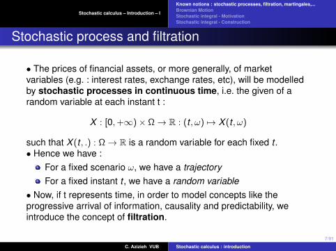
Stochastic process and filtration
• The prices of financial assets, or more generally, of marketvariables (e.g. : interest rates, exchange rates, etc), will be modelledby stochastic processes in continuous time, i.e. the given of arandom variable at each instant t :
X : [0,+∞)× Ω→ R : (t , ω) 7→ X (t , ω)
such that X (t , .) : Ω→ R is a random variable for each fixed t .• Hence we have :
For a fixed scenario ω, we have a trajectoryFor a fixed instant t , we have a random variable
• Now, if t represents time, in order to model concepts like theprogressive arrival of information, causality and predictability, weintroduce the concept of filtration.
C. Azizieh VUB Stochastic calculus : introduction
8/91
Stochastic calculus – Introduction – I
Known notions : stochastic processes, filtration, martingales,...Brownian MotionStochastic integral - MotivationStochastic integral - Construction
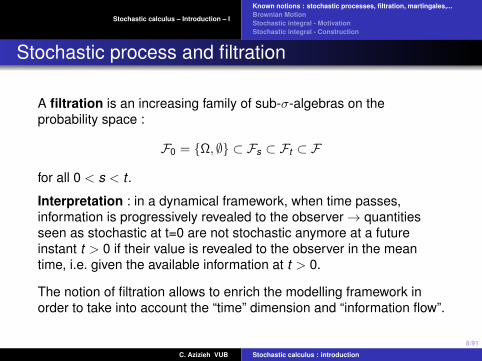
Stochastic process and filtration
A filtration is an increasing family of sub-σ-algebras on theprobability space :
F0 = Ω, ∅ ⊂ Fs ⊂ Ft ⊂ F
for all 0 < s < t .
Interpretation : in a dynamical framework, when time passes,information is progressively revealed to the observer→ quantitiesseen as stochastic at t=0 are not stochastic anymore at a futureinstant t > 0 if their value is revealed to the observer in the meantime, i.e. given the available information at t > 0.
The notion of filtration allows to enrich the modelling framework inorder to take into account the “time” dimension and “information flow”.
C. Azizieh VUB Stochastic calculus : introduction

9/91
Stochastic calculus – Introduction – I
Known notions : stochastic processes, filtration, martingales,...Brownian MotionStochastic integral - MotivationStochastic integral - Construction
Filtration and process
Notions linked by two definitions :
Definition (Natural filtration or filtration generated by a stochasticprocess)
Every stochastic process X generates a filtration called the “naturalfiltration” of the process, and defined by :
Ft = σ(X (s)|s ≤ t) ∀t
(filtration corresponding to the history of the process)
Definition (Adapted process)
A process X is said to be adapted to a filtration (Ft ) if
X (t) is Ft – measurable ∀t
C. Azizieh VUB Stochastic calculus : introduction

10/91
Stochastic calculus – Introduction – I
Known notions : stochastic processes, filtration, martingales,...Brownian MotionStochastic integral - MotivationStochastic integral - Construction
Filtration and process
Concretely, if (Ft ) represents the available information (in a market)through time, a process (Xt ) is adapted if its value at t is known assoon as we have reach instant t .
In finance, we will model prices of financial assets by adaptedprocesses.
Definition
A filtration Ft is said to satisfy the usual conditions ifF0 contains all sets of zero probability∀t ≥ 0 Ft = ∩
s>tFs (right continuous).
In what follows, we will always assume that the filtration satisfies theusual conditions (...)
C. Azizieh VUB Stochastic calculus : introduction

11/91
Stochastic calculus – Introduction – I
Known notions : stochastic processes, filtration, martingales,...Brownian MotionStochastic integral - MotivationStochastic integral - Construction
Continuous stochastic processA continuous stochastic process is such that t → Xt (ω) is continuousfor all ω ∈ Ω0 ⊂ Ω with P [Ω0] = 1.
In other words : a process whose trajectories are almost allcontinuous.
0 0.5 1 1.5 2 2.5 3 3.5 4 4.5 5-2
-1.5
-1
-0.5
0
0.5
1
1.5
Time t
X(t
)
C. Azizieh VUB Stochastic calculus : introduction

12/91
Stochastic calculus – Introduction – I
Known notions : stochastic processes, filtration, martingales,...Brownian MotionStochastic integral - MotivationStochastic integral - Construction
Continuous time martingale
The notion of martingale is central in market finance.
Definition (continuous time martingale)
A stochastic process (Mt )t≥0 is a martingale w.r.t. a filtration Ftt iffor all t :
1 Mt is Ft -measurable (adapted process)2 Mt is integrable (hence IE [|Mt |] <∞)3 IE [Mt |Fs ] = Ms for all s < t .
Interpretation : accumulated gains of a player in an equilibrated game
In particular, E [Mt ] = M0.
C. Azizieh VUB Stochastic calculus : introduction
13/91
Stochastic calculus – Introduction – I
Known notions : stochastic processes, filtration, martingales,...Brownian MotionStochastic integral - MotivationStochastic integral - Construction
Martingales - Doob’s results in continuous time
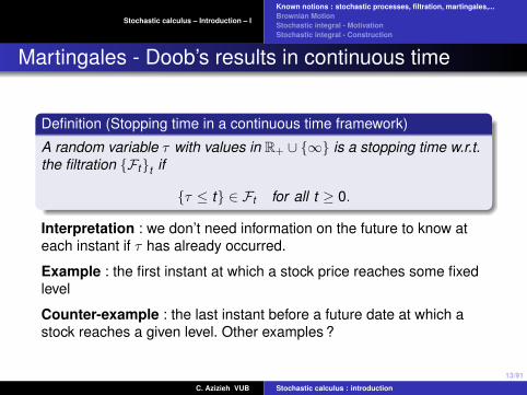
Definition (Stopping time in a continuous time framework)
A random variable τ with values in R+ ∪ ∞ is a stopping time w.r.t.the filtration Ftt if
τ ≤ t ∈ Ft for all t ≥ 0.
Interpretation : we don’t need information on the future to know ateach instant if τ has already occurred.
Example : the first instant at which a stock price reaches some fixedlevel
Counter-example : the last instant before a future date at which astock reaches a given level. Other examples ?
C. Azizieh VUB Stochastic calculus : introduction

14/91
Stochastic calculus – Introduction – I
Known notions : stochastic processes, filtration, martingales,...Brownian MotionStochastic integral - MotivationStochastic integral - Construction
Martingales - Doob’s results in continuous time
An example of link between stopping time and stochastic process :
Definition (Process stopped by a stopping time)
Let (Yt )t be an adapted process to the filtration Ftt and let τ be astopping time. The process stopped at instant τ , denoted by (Y τ
t )t or
(Yt∧τ )t is defined by
Y τt (ω) = Yt∧τ(ω) (ω) ∀t .
C. Azizieh VUB Stochastic calculus : introduction

15/91
Stochastic calculus – Introduction – I
Known notions : stochastic processes, filtration, martingales,...Brownian MotionStochastic integral - MotivationStochastic integral - Construction
Martingales - Doob’s results in continuous time
Example :
Let Y be a stochastic process and let us define the stopping time :
T = inft ≥ 0|Y (t) ≥ M
for M ∈ R (M = barrier). The process Y stopped at M is then :
Z (t) = Y (t ∧ T ) =
Y (t) if t ≤ TM if t > T
C. Azizieh VUB Stochastic calculus : introduction

16/91
Stochastic calculus – Introduction – I
Known notions : stochastic processes, filtration, martingales,...Brownian MotionStochastic integral - MotivationStochastic integral - Construction
Martingales - Doob’s results in continuous time
When we stop a (continuous) martingale with a stopping time, we stillhave a (continuous) martingale :
Theorem (Doob’s stopping time theorem)
Let (Mt )t be a continuous martingale w.r.t. filtration Ft.Let τ be a stopping time w.r.t. Ft .Then the process Xt = Mt∧τ is a continuous martingale w.r.t. Ft .
Proof : see [Steele, section 4.4].
C. Azizieh VUB Stochastic calculus : introduction

17/91
Stochastic calculus – Introduction – I
Known notions : stochastic processes, filtration, martingales,...Brownian MotionStochastic integral - MotivationStochastic integral - Construction
Martingales - Doob’s results in continuous time
Theorem (Doob’s maximal inequalities in continuous time)
Let (Mt )t be a continuous non-negative sub-martingale and λ > 0..Then for all p ≥ 1, we have :
λpP
(sup
t :0≤t≤TMt > λ
)≤ IE
[Mp
T
](1)
and, if MT ∈ Lp (dP) for some p > 1, then :∥∥∥∥∥ supt :0≤t≤T
Mt
∥∥∥∥∥p
≤ pp − 1
‖MT‖p . (2)
Proof : see [Steele, section 4.4].
C. Azizieh VUB Stochastic calculus : introduction

18/91
Stochastic calculus – Introduction – I
Known notions : stochastic processes, filtration, martingales,...Brownian MotionStochastic integral - MotivationStochastic integral - Construction
Convergence of random variables
Let Xn|n ∈ IN be a sequence of random variables.
What is limn→∞ Xn ? ?
One can actually define different types of convergence :almost sure convergencequadratic convergence (or L2)convergence in probabilityconvergence in distributionconvergence in Lp norm...
C. Azizieh VUB Stochastic calculus : introduction

19/91
Stochastic calculus – Introduction – I
Known notions : stochastic processes, filtration, martingales,...Brownian MotionStochastic integral - MotivationStochastic integral - Construction
Almost sure convergence
Xnp.s.→ X iff P[ω ∈ Ω|Xn(ω)→ X (ω)] = 1
Example : Strong law of large numbers :
If (Xn) is a sequence of random variables i.i.d. with finite expectationIE [X1] = µ, then :
1n
n∑i=1
Xip.s.→ E [X1] = µ
C. Azizieh VUB Stochastic calculus : introduction
20/91
Stochastic calculus – Introduction – I
Known notions : stochastic processes, filtration, martingales,...Brownian MotionStochastic integral - MotivationStochastic integral - Construction
Quadratic convergence (or in L2)
Xn → X in quadratic mean (or in L2) iff
‖Xn − X‖2L2 = IE [(Xn − X )2] =
∫Ω
(Xn(ω)− X (ω))2dP(ω)→ 0
C. Azizieh VUB Stochastic calculus : introduction

21/91
Stochastic calculus – Introduction – I
Known notions : stochastic processes, filtration, martingales,...Brownian MotionStochastic integral - MotivationStochastic integral - Construction
Convergence in probability
XnP→ X iff ∀ε > 0 : P[ω ∈ Ω : |Xn(ω)− X (ω)| ≥ ε]→ 0
Link between these different types of convergence :
• Almost sure convergence⇒ convergence in probability
• Convergence in L2 ⇒ convergence in probability
C. Azizieh VUB Stochastic calculus : introduction

22/91
Stochastic calculus – Introduction – I
Known notions : stochastic processes, filtration, martingales,...Brownian MotionStochastic integral - MotivationStochastic integral - Construction
Convergence in distribution
XnD→ X iff ∀f bounded continuous : E [f (Xn)]→ E [f (X )]
In particular this is equivalent to the convergence of characteristicfunctions :
Definition : characteristic function of a random variable X :
∀z ∈ R : ΦX (z) := E [exp(izX )] =
∫Ω
eizX(ω)dP(ω) =
∫R
eizxdµX (x)
(characteristic function = inverse Fourier transform of the density of Xif X has such a density (up to some normalization constant)...)
Result : (Xn) converges in distribution iff we have convergence ofcharacteristic functions :
XnD→ X iff ΦXn (z)→ ΦX (z) for all z ∈ R
C. Azizieh VUB Stochastic calculus : introduction

23/91
Stochastic calculus – Introduction – I
Known notions : stochastic processes, filtration, martingales,...Brownian MotionStochastic integral - MotivationStochastic integral - Construction
Convergence in distribution
convergence in probability⇒ convergence in distribution
Theorem (Central limit theorem)
If (Xn) is a sequence of i.i.d. random variables with finite variance σ2,then ∑n
i=1 Xi − nE [X1]
σ√
nD→ N(0,1)
C. Azizieh VUB Stochastic calculus : introduction

24/91
Stochastic calculus – Introduction – I
Known notions : stochastic processes, filtration, martingales,...Brownian MotionStochastic integral - MotivationStochastic integral - Construction
Brownian motion : Motivation
Suppose that we would like to define a stochastic model for theevolution of a financial asset in continuous time.
Discrete time Continuous time
Deterministic model Sn = S0(1 + i)n S(t) = S0eδt
Stochastic model Sn = S0∏n
k=1(1 + ik ) ? ?
C. Azizieh VUB Stochastic calculus : introduction

25/91
Stochastic calculus – Introduction – I
Known notions : stochastic processes, filtration, martingales,...Brownian MotionStochastic integral - MotivationStochastic integral - Construction
Brownian Motion : Motivation
Continuous deterministic model
We consider a financial asset which evolves deterministically in time :constant rate of return : δvalue of the asset at t : S(t)we assume a double linearity hypothesis :
∆S(t) = δS(t)∆t
→ the evolution of the price is supposed to be proportional to timeand to the invested amount
C. Azizieh VUB Stochastic calculus : introduction

26/91
Stochastic calculus – Introduction – I
Known notions : stochastic processes, filtration, martingales,...Brownian MotionStochastic integral - MotivationStochastic integral - Construction
Brownian Motion : Motivation
Continuous deterministic model
• If we take the limit for ∆t → 0, we obtain the differential equation :
dS(t) = δS(t)dt
whose solution (passing by (0,S(0))) is given by the exponential function :
S(t) = S(0)eδt
• Now, if we assume that the rate of return is not constant anymore, i.e. ifδ = δ(t), then the differential equation becomes :
dS(t) = δ(t)S(t)dt
whose solution is given by :
S(t) = S(0)e∫ t
0 δ(s)ds
C. Azizieh VUB Stochastic calculus : introduction
27/91
Stochastic calculus – Introduction – I
Known notions : stochastic processes, filtration, martingales,...Brownian MotionStochastic integral - MotivationStochastic integral - Construction
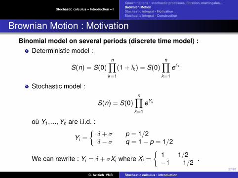
Brownian Motion : MotivationBinomial model on several periods (discrete time model) :
Deterministic model :
S(n) = S(0)n∏
k=1
(1 + ik ) = S(0)n∏
k=1
eδk
Stochastic model :
S(n) = S(0)n∏
k=1
eYk
ou Y1, ...,Yn are i.i.d. :
Yi =
δ + σ p = 1/2δ − σ q = 1− p = 1/2
We can rewrite : Yi = δ + σXi where Xi =
1 1/2−1 1/2 .
C. Azizieh VUB Stochastic calculus : introduction

28/91
Stochastic calculus – Introduction – I
Known notions : stochastic processes, filtration, martingales,...Brownian MotionStochastic integral - MotivationStochastic integral - Construction
Brownian Motion : Motivation
We hence have :
S(n) = S(0)n∏
k=1
eδ+σXk = S(0)enδ+σ∑n
k=1 Xk
We hence obtain the cumulative log-return until n :
log(S(n)/S(0)) =n∑
i=1
Yi = δn︸︷︷︸determ. trend
+ σ
n∑i=1
Xi︸ ︷︷ ︸random walk
In particular, the moments of cumulative log-returns are given by :E[log(S(n)/S(0))] = δnvar [log(S(n)/S(0))] = σ2n
(variance proportional to time)C. Azizieh VUB Stochastic calculus : introduction

29/91
Stochastic calculus – Introduction – I
Known notions : stochastic processes, filtration, martingales,...Brownian MotionStochastic integral - MotivationStochastic integral - Construction
Brownian Motion : Motivation
We will now consider passing to a continuous time model.
This will be done in two steps :1 Modification of the (space and time) scale of the random
walk :The time periods of 1 are replaced by ∆t , and jumps of +1 and -1are replaced by jumps of +∆x and −∆x on each period of time.
The random walk then becomes :
W (n) = ∆x .m∑
i=1
Xi , with m = n/∆t
and in terms of moments :E[W (n)] = 0Var [W (n)] = m(∆x)2 = n (∆x)2
∆t
C. Azizieh VUB Stochastic calculus : introduction

30/91
Stochastic calculus – Introduction – I
Known notions : stochastic processes, filtration, martingales,...Brownian MotionStochastic integral - MotivationStochastic integral - Construction
Brownian Motion : Motivation
2 Passing to the limit ∆x ,∆t → 0
We will now consider a sequence of ∆xk ,∆tk with ∆xk ,∆tk → 0in such a way that the limiting process is non-trivial.For this purpose, we will require :
(∆xk )2
∆tk→ 1
(and not ∆xk∆tk→ 1 !)
C. Azizieh VUB Stochastic calculus : introduction

31/91
Stochastic calculus – Introduction – I
Known notions : stochastic processes, filtration, martingales,...Brownian MotionStochastic integral - MotivationStochastic integral - Construction
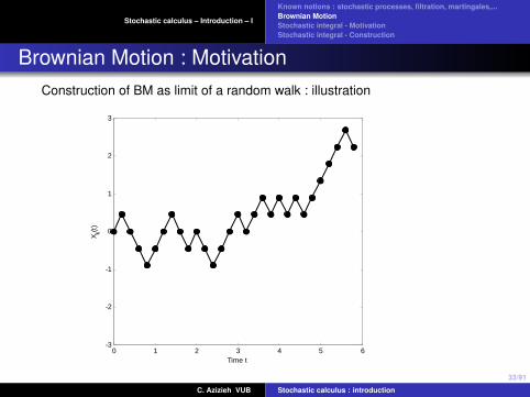
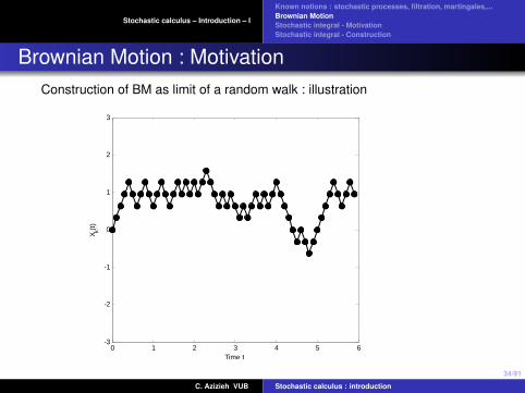
Brownian Motion : MotivationConstruction of BM as limit of a random walk : illustration
0 1 2 3 4 5 6-3
-2
-1
0
1
2
3
Time t
X k(t)
C. Azizieh VUB Stochastic calculus : introduction

32/91
Stochastic calculus – Introduction – I
Known notions : stochastic processes, filtration, martingales,...Brownian MotionStochastic integral - MotivationStochastic integral - Construction
Brownian Motion : MotivationConstruction of BM as limit of a random walk : illustration
0 1 2 3 4 5 6-3
-2
-1
0
1
2
3
Time t
X k(t)
C. Azizieh VUB Stochastic calculus : introduction
33/91
Stochastic calculus – Introduction – I
Known notions : stochastic processes, filtration, martingales,...Brownian MotionStochastic integral - MotivationStochastic integral - Construction
Brownian Motion : MotivationConstruction of BM as limit of a random walk : illustration
0 1 2 3 4 5 6-3
-2
-1
0
1
2
3
Time t
X k(t)
C. Azizieh VUB Stochastic calculus : introduction
34/91
Stochastic calculus – Introduction – I
Known notions : stochastic processes, filtration, martingales,...Brownian MotionStochastic integral - MotivationStochastic integral - Construction
Brownian Motion : MotivationConstruction of BM as limit of a random walk : illustration
0 1 2 3 4 5 6-3
-2
-1
0
1
2
3
Time t
X k(t)
C. Azizieh VUB Stochastic calculus : introduction

35/91
Stochastic calculus – Introduction – I
Known notions : stochastic processes, filtration, martingales,...Brownian MotionStochastic integral - MotivationStochastic integral - Construction
Brownian Motion : MotivationConstruction of BM as limit of a random walk : illustration
0 1 2 3 4 5 6-3
-2
-1
0
1
2
3
Time t
X k(t)
C. Azizieh VUB Stochastic calculus : introduction

36/91
Stochastic calculus – Introduction – I
Known notions : stochastic processes, filtration, martingales,...Brownian MotionStochastic integral - MotivationStochastic integral - Construction
Brownian Motion : MotivationConstruction of BM as limit of a random walk : illustration
0 1 2 3 4 5 6-3
-2
-1
0
1
2
3
Time t
X k(t)
C. Azizieh VUB Stochastic calculus : introduction

37/91
Stochastic calculus – Introduction – I
Known notions : stochastic processes, filtration, martingales,...Brownian MotionStochastic integral - MotivationStochastic integral - Construction
Brownian Motion : MotivationConstruction of BM as limit of a random walk : illustration
0 1 2 3 4 5 6-3
-2
-1
0
1
2
3
Time t
X k(t)
C. Azizieh VUB Stochastic calculus : introduction

38/91
Stochastic calculus – Introduction – I
Known notions : stochastic processes, filtration, martingales,...Brownian MotionStochastic integral - MotivationStochastic integral - Construction
Brownian Motion : MotivationConstruction of BM as limit of a random walk : illustration
0 1 2 3 4 5 6-3
-2
-1
0
1
2
3
Time t
X k(t)
C. Azizieh VUB Stochastic calculus : introduction

39/91
Stochastic calculus – Introduction – I
Known notions : stochastic processes, filtration, martingales,...Brownian MotionStochastic integral - MotivationStochastic integral - Construction
Brownian Motion : Motivation
One can show that the sequence of processes (W (k)(t)) definedabove converges in distribution to a process with continuoustrajectories called Brownian motion :
W (k)(t) = ∆xk
t/∆tk∑i=1
Xi →W (t)
where W (t) :is a continuous time processis called
Standard Brownian motion, orWiener process, or”infinitesimal random walk”
C. Azizieh VUB Stochastic calculus : introduction

40/91
Stochastic calculus – Introduction – I
Known notions : stochastic processes, filtration, martingales,...Brownian MotionStochastic integral - MotivationStochastic integral - Construction
Brownian Motion : Motivation
This convergence is actually the dynamic equivalent of the centrallimit theorem in the static case :
If (Xn) is a sequence of i.i.d. random variables of mean µ and finitevariance σ2, then we note Sn =
∑ni=1 Xi ,
Sn − nµσ√
nD→ N(0,1)
C. Azizieh VUB Stochastic calculus : introduction

41/91
Stochastic calculus – Introduction – I
Known notions : stochastic processes, filtration, martingales,...Brownian MotionStochastic integral - MotivationStochastic integral - Construction
Brownian Motion : Motivation
By construction, this process W (t) has the following properties :
(i) E[W (k)(t)] = 0→ E[W (t)] = 0
(ii) var [W (k)(t)] = t (∆Xk )2
∆tk→ var [W (t)] = t
(iii) W (k)(t) = sum of i.i.d. rvs→W (t) ∼ N(0, t) (Central LimitTheorem)
(iv) W is a process with independent and stationary increments
C. Azizieh VUB Stochastic calculus : introduction
42/91
Stochastic calculus – Introduction – I
Known notions : stochastic processes, filtration, martingales,...Brownian MotionStochastic integral - MotivationStochastic integral - Construction
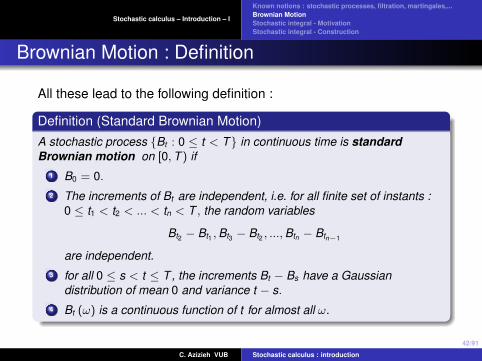
Brownian Motion : Definition
All these lead to the following definition :
Definition (Standard Brownian Motion)A stochastic process Bt : 0 ≤ t < T in continuous time is standardBrownian motion on [0,T ) if
1 B0 = 0.2 The increments of Bt are independent, i.e. for all finite set of instants :
0 ≤ t1 < t2 < ... < tn < T , the random variables
Bt2 − Bt1 ,Bt3 − Bt2 , ...,Btn − Btn−1
are independent.3 for all 0 ≤ s < t ≤ T , the increments Bt − Bs have a Gaussian
distribution of mean 0 and variance t − s.4 Bt (ω) is a continuous function of t for almost all ω.
C. Azizieh VUB Stochastic calculus : introduction
43/91
Stochastic calculus – Introduction – I
Known notions : stochastic processes, filtration, martingales,...Brownian MotionStochastic integral - MotivationStochastic integral - Construction
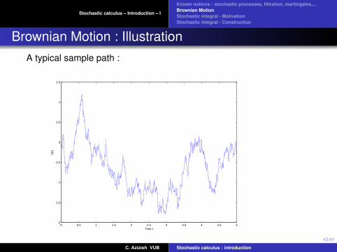
Brownian Motion : IllustrationA typical sample path :
0 0.5 1 1.5 2 2.5 3 3.5 4 4.5 5-2
-1.5
-1
-0.5
0
0.5
1
1.5
Time t
X(t
)
It can be shown that the sample paths (a.s.) are nowheredifferentiable
C. Azizieh VUB Stochastic calculus : introduction

44/91
Stochastic calculus – Introduction – I
Known notions : stochastic processes, filtration, martingales,...Brownian MotionStochastic integral - MotivationStochastic integral - Construction
Brownian Motion : back to the stochastic continuousmodel
The random walk W (k)(t) converges to the standard Brownian motionW (t).
The price of the asset S(t) hence becomes at the limit :
S(k)(t) = S(0)etδ+σ∆xk∑t/∆tk
k=1 Xk
↓
S(t) = S(0)eδt+σW (t)
This is what will be called later geometric Brownian motion.
C. Azizieh VUB Stochastic calculus : introduction

45/91
Stochastic calculus – Introduction – I
Known notions : stochastic processes, filtration, martingales,...Brownian MotionStochastic integral - MotivationStochastic integral - Construction
Brownian Motion : Historical Perspective
1829 : Brown : movement of pollen particles in suspension1900 : Bachelier models financial stock prices by a Brownianmotion1905 : Einstein models particles in suspension in a liquid or agaz, subject to collisions1923 : Wiener proposes a rigorous construction of Brownianmotion (also called “Wiener process”)1944 : Ito contributes to define a stochastic integral w.r.t. aBrownian motion
BM has become a central process in finance for modelling theuncertainty present in the markets
C. Azizieh VUB Stochastic calculus : introduction

46/91
Stochastic calculus – Introduction – I
Known notions : stochastic processes, filtration, martingales,...Brownian MotionStochastic integral - MotivationStochastic integral - Construction
Brownian motion and the Markov property
By using the independence of disjoint increments we directly obtain :
P[Xt+s ∈ B |Xu,0 ≤ u ≤ t ] = P[Xt+s ∈ B |Xt ].
i.e. Markov property .
We also get :
P[Xt+s ∈ B |Xt = x ] = P[Xt+s − Xt ∈ B − x |Xt − X0 = x ]
= P[Xt+s − Xt ∈ B − x ] = P[Xt+s − Xt + x ∈ B] = P[Y ∈ B],
where Y ∼ N (x , s). We also have :
P[Xt+s ∈ B |Xt = x ] =
∫B
1√2πs
e−(y−x)2/(2s) dy .
C. Azizieh VUB Stochastic calculus : introduction

47/91
Stochastic calculus – Introduction – I
Known notions : stochastic processes, filtration, martingales,...Brownian MotionStochastic integral - MotivationStochastic integral - Construction
Non standard Brownian Motion
Brownian motion from level a
Z (t) = a + B(t)
where (Bt ) is a standard BM
Brownian motion from level a, with drift µ and volatility σ
Z (t) = a + µt + σBt
In particular,E [Z (t)] = a + µt
var [Z (t)] = σ2t
C. Azizieh VUB Stochastic calculus : introduction

48/91
Stochastic calculus – Introduction – I
Known notions : stochastic processes, filtration, martingales,...Brownian MotionStochastic integral - MotivationStochastic integral - Construction
Brownian motion and Gaussian processes
Definition ( Gaussian processes)
Xt : 0 ≤ t <∞ is a Gaussian process iff every linear combination ofvalues of X at different instants is normally distributed :
n∑k=1
αk Xtk
has a normal distribution for all coefficients αk and instants tk .
Remark : such a process is characterized by :a mean function t 7→ E[Xt ] andan autocovariance function (s, t) 7→ Cov[Xs,Xt ].
Example of Gaussian process : Brownian motion.
C. Azizieh VUB Stochastic calculus : introduction

49/91
Stochastic calculus – Introduction – I
Known notions : stochastic processes, filtration, martingales,...Brownian MotionStochastic integral - MotivationStochastic integral - Construction
Brownian motion and Gaussian processes
Let us compute the covariance function of a Brownian motion.
for all s ≤ t :
cov (Bs,Bt ) = IE [(Bt − Bs + Bs) Bs] = IE [Bt−Bs]IE [Bs]+IE[B2
s]
= IE[B2
s]
= s
=⇒ cov (Bs,Bt ) = min (s, t) 0 ≤ s, t <∞.
C. Azizieh VUB Stochastic calculus : introduction

50/91
Stochastic calculus – Introduction – I
Known notions : stochastic processes, filtration, martingales,...Brownian MotionStochastic integral - MotivationStochastic integral - Construction
Brownian motion and Gaussian processes
Lemma
Let Xt : 0 ≤ t ≤ T be a Gaussian process with IE [Xt ] = 0 for all0 ≤ t ≤ T and let cov (Xs,Xt ) = min (s, t) for all 0 ≤ s, t ≤ T , then theprocess Xt has independent increments.
Moreover, if the process has continuous trajectories and X0 = 0, thenXtt is a standard Brownian motion on [0,T ] .
C. Azizieh VUB Stochastic calculus : introduction

51/91
Stochastic calculus – Introduction – I
Known notions : stochastic processes, filtration, martingales,...Brownian MotionStochastic integral - MotivationStochastic integral - Construction
Martingales and Brownian motion
Theorem
Let (Bt ) be a standard Brownian motion. Then :1 (Bt )t2(B2
t − t)
t3(exp
(αBt − α2t/2
))t
are martingales w.r.t. a Ftt (= the family of sub-sigma algebraσ (Bs, s ≤ t) completed by adding the sets of zero probability).
C. Azizieh VUB Stochastic calculus : introduction

52/91
Stochastic calculus – Introduction – I
Known notions : stochastic processes, filtration, martingales,...Brownian MotionStochastic integral - MotivationStochastic integral - Construction
Martingales and Brownian motion
Proof1) Bt Ft -measurable,
IE[B2
t]
= t <∞,IE [Bt − Bs |Fs ] = 0 since IE [Bt − Bs] = 0.
2)(B2
t − t)Ft -measurable,
IE[∣∣B2
t − t∣∣] ≤ IE [B2
t ] + t = 2t ,
IE[B2
t − t |Fs]
= IE[(Bt − Bs)2 − B2
s + 2BtBs − t |Fs
]= IE
[(Bt−s)2 |Fs
]− t − B2
s + 2B2s
= t − s − t + B2s = B2
s − s.
3) IE[exp
(αBt − α2t/2
)|Fs]
= IE[exp
(α (Bt − Bs)− α2
2 (t − s))|Fs
]exp
(αBs − α2s
2
)= IE [exp (αBt−s)] exp
(−α
2
2 (t − s))
exp(αBs − α2s
2
)= exp
(αBs − α2s
2
).
C. Azizieh VUB Stochastic calculus : introduction

53/91
Stochastic calculus – Introduction – I
Known notions : stochastic processes, filtration, martingales,...Brownian MotionStochastic integral - MotivationStochastic integral - Construction
Martingales and Brownian motion
Remark :We can actually show that the converse is also true : if (Xt ) is acontinuous process such that (Xt ) and (X 2
t − t) are martingales andX (0) = 0, then (Xt ) is a standard Brownian motion
Brownian motion appears as the fundamental example of continuousmartingale
C. Azizieh VUB Stochastic calculus : introduction

54/91
Stochastic calculus – Introduction – I
Known notions : stochastic processes, filtration, martingales,...Brownian MotionStochastic integral - MotivationStochastic integral - Construction
Brownian motion and bounded variation
Let us consider a sequence of subdivisions of interval [0,t] :0 = t0 < t1 < ... < tn = t with thikness tending to 0(limn→∞max0≤i≤n |ti+1 − ti | = 0).We know that
E
[n∑
i=1
(∆B(ti ))2
]=
n∑i=1
∆ti = t .
If f is a deterministic function with bounded variation, limn→∞∑n
i=1 |∆f (ti )|exists, and
limn→∞
n∑i=1
(∆f (ti ))2 = 0.
This implies that trajectories of a Brownian motion cannot be of boundedvariation. In particular, they cannot be differentiable (in the classical sense).Hence, these trajectories are continuous everywhere but nowheredifferentiable.
C. Azizieh VUB Stochastic calculus : introduction
55/91
Stochastic calculus – Introduction – I
Known notions : stochastic processes, filtration, martingales,...Brownian MotionStochastic integral - MotivationStochastic integral - Construction
Brownian motion and quadratic variation
Lemma (Quadratic variation of a BM)
Let tj = j2n t (j = 0, ...,2n) be a partition of [0,t]. Then
Zn =2n∑
j=1
(B(tj )− B(tj−1))2 → t in L2
Proof(i) E[Zn] = t(ii) IE [(Zn − t)2] = Var [Zn] =
∑2n
j=1 Var(∆B(tj )2).
Now, if X ∼ N(0, σ2), then Var(X 2) = 2σ4 (exercise), which implies :
Var(Zn) =2n∑
j=1
2(
t2n
)2
= 2n+1 t2
22n → 0.
C. Azizieh VUB Stochastic calculus : introduction

56/91
Stochastic calculus – Introduction – I
Known notions : stochastic processes, filtration, martingales,...Brownian MotionStochastic integral - MotivationStochastic integral - Construction
Stochastic integral - Motivation
Let us consider a market composed of d assets of price at t :St = (S1
t , ...,Sdt ), modeled like a vector process
A trading strategy can be modelled by a vector φt describing thequantities invested in each of the assets at instant t : φt = (φ1
t , ..., φdt )
The value at t of the portfolio obtained by following this strategy is thengiven by :
Vt (φ) =d∑
k=1
φkt Sk
t = φt .St
We will denote by 0 = T0,T1, ...,Tn+1 = T the rebalancing instants :between 2 such instants, the composition of the portfolio is supposedunchanged.
C. Azizieh VUB Stochastic calculus : introduction

57/91
Stochastic calculus – Introduction – I
Known notions : stochastic processes, filtration, martingales,...Brownian MotionStochastic integral - MotivationStochastic integral - Construction
Stochastic integral - Motivation
We can then denote by φi = (φ1i , ..., φ
di ) the composition of the portfolio
between Ti and Ti+1, and rewrite φt as :
φt = φ0It=0 +n∑
i=0
φiI]Ti ,Ti+1] (∗)
Generally, the rebalancing instants Ti are random (depending e.g. fromthe levels reached by some assets in the market...). The strategy φt
appears as a Stochastic process.
Definition (Simple predictable process)
A process φt (t ∈ [0,T ]) that can be represented by (∗) is called a simplepredictable process if moreover the stochastic instants Ti are stoppingtimes , and if φi are bounded random variables with φi ∈ FTi , (which meansthat the value φi is revealed at instant Ti ).
C. Azizieh VUB Stochastic calculus : introduction

58/91
Stochastic calculus – Introduction – I
Known notions : stochastic processes, filtration, martingales,...Brownian MotionStochastic integral - MotivationStochastic integral - Construction
Stochastic integral - MotivationExample of simple predictable process (one of its component) :
C. Azizieh VUB Stochastic calculus : introduction

59/91
Stochastic calculus – Introduction – I
Known notions : stochastic processes, filtration, martingales,...Brownian MotionStochastic integral - MotivationStochastic integral - Construction
Stochastic integral - Motivation
Gain process for a simple trading strategy
If φt is simple (we speak about simple trading strategy), then thegain realized by the trader between Ti and Ti+1 is equal to thescalar product
φi .(STi+1 − STi )
Hence the accumulated gain on [0,T ] of the trader beginningwith an initial composition given by φ0 can be written as :
GT (φ) = φ0.S0 +n∑
i=0
φi .(STi+1 − STi )
C. Azizieh VUB Stochastic calculus : introduction

60/91
Stochastic calculus – Introduction – I
Known notions : stochastic processes, filtration, martingales,...Brownian MotionStochastic integral - MotivationStochastic integral - Construction
Stochastic integral - Motivation
Definition (Stochastic integral of a simple predictable process)
GT is called the stochastic integral of the simple predictableprocess φ w.r.t. the price process (St ), and will be denoted by :∫ T
0φ(u).dS(u)
In finance, the cumulative gains of a trader following a strategylead naturally to a new concept of integral : the stochasticintegral
C. Azizieh VUB Stochastic calculus : introduction

61/91
Stochastic calculus – Introduction – I
Known notions : stochastic processes, filtration, martingales,...Brownian MotionStochastic integral - MotivationStochastic integral - Construction
Stochastic integral - Motivation
In view of getting some results concerning option prices in given modelswe cannot limit ourselves to the case where φ is a simple strategy.Hence we need to give a sense to this stochastic integral / gain process,also in the case where the composition continuously changes with time.
We will first give a sense to this integral in the case where St is aBrownian motion of dimension 1, and in the case where φt is a moregeneral process (not necessarily simple) :∫ t
0φ(s)dBs
C. Azizieh VUB Stochastic calculus : introduction

62/91
Stochastic calculus – Introduction – I
Known notions : stochastic processes, filtration, martingales,...Brownian MotionStochastic integral - MotivationStochastic integral - Construction
Stochastic integral - Motivation
A first naive idea would consist to define the stochastic integralas a limit obtained along each trajectory :(∫ t
0φ(s)dBs
)(ω) = lim
max(ti−ti−1)→0
n∑i=1
φti−1 (ω)[Bti (ω)− Bti−1 (ω)
]The problem is that (almost all) trajectories of a Brownian motionhave no bounded variation... and that this limit hence does notexist in general for a given trajectory !
C. Azizieh VUB Stochastic calculus : introduction

63/91
Stochastic calculus – Introduction – I
Known notions : stochastic processes, filtration, martingales,...Brownian MotionStochastic integral - MotivationStochastic integral - Construction
Ito integral - Construction
The stochastic integral will be defined as a limit of Riemann sums, butnot in the sense of a.s. convergence, but in quadratic convergence(L2)
Objective : give a mathematical sense to :
I (X ) (ω) =∫ T
0 X (ω, t) dBt .
where X (t) is a general stochastic process.
C. Azizieh VUB Stochastic calculus : introduction

64/91
Stochastic calculus – Introduction – I
Known notions : stochastic processes, filtration, martingales,...Brownian MotionStochastic integral - MotivationStochastic integral - Construction
Stochastic integral - Construction
Contrarily to the Riemann integral, the result can depend on thepoint yi ∈ [ti−1, ti ). In the Ito integral, we will fix yi = ti−1 ;The final objective is to develop an integral allowing to introduceand to study stochastic evolution equations in continuous time(→ Stochastic differential equations, describing the dynamics ofmarket variables)
C. Azizieh VUB Stochastic calculus : introduction

65/91
Stochastic calculus – Introduction – I
Known notions : stochastic processes, filtration, martingales,...Brownian MotionStochastic integral - MotivationStochastic integral - Construction
Stochastic integral - Construction
Notations
B [0,T ] = the set of Borel sets on [0,T ] (Borel sigma-algebra, i.e.the smallest σ−algebra containing all open sets in [0,T ] .)Ftt the standard Brownian filtration.for all fixed t : Ft ⊗ B = the smallest σ−algebra containing theproduct sets A× B ou A ∈ Ft and B ∈ B.
We say that a stochastic process X (., .) is measurable if X (., .) isFT ⊗ B-measurable.
We say that a process X (., .) is adapted if X (., t) ∈ Ft , ∀t ∈ (0,T ).
C. Azizieh VUB Stochastic calculus : introduction

66/91
Stochastic calculus – Introduction – I
Known notions : stochastic processes, filtration, martingales,...Brownian MotionStochastic integral - MotivationStochastic integral - Construction
Stochastic integral - Construction
In summary, Ito stochastic integral will be defined by following thesubsequent steps :
Definition of Ito integral for a simple processIto isometry : the stochastic integral preserves the L2 norm (inother words, is continuous for that norm)Density of the set of simple processes within the set of adaptedsquare-integrable stochastic processes (with the L2)Extension by density of the Ito integral on the set ofsquare-integrable adapted stochastic processes thanks to the Itoisometry
C. Azizieh VUB Stochastic calculus : introduction
67/91
Stochastic calculus – Introduction – I
Known notions : stochastic processes, filtration, martingales,...Brownian MotionStochastic integral - MotivationStochastic integral - Construction
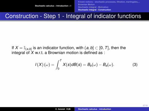
Construction - Step 1 - Integral of indicator functions
If X = I(a,b] is an indicator function, with (a,b] ⊂ [0,T ], then theintegral of X w.r.t. a Brownian motion is defined as :
I (X ) (ω) =
∫ T
0X (s)dB(s) = Bb(ω)− Ba(ω). (3)
C. Azizieh VUB Stochastic calculus : introduction
68/91
Stochastic calculus – Introduction – I
Known notions : stochastic processes, filtration, martingales,...Brownian MotionStochastic integral - MotivationStochastic integral - Construction
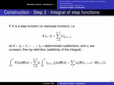
Construction - Step 2 - Integral of step functions
If X is a step function (or staircase function), i.e.
X (ω, t) =n−1∑i=0
ciI]ti ,ti+1]
ou 0 = t0 < t1 < ... < tn = deterministic subdivision, and ci areconstant, then by definition (additivity of the integral) :
∫ T
0X (s)dB(s) =
n−1∑i=0
ci
∫ T
0I]ti ,ti+1](s)dB(s) =
∑i
ci (B(ti+1, ω)−B(ti , ω))
C. Azizieh VUB Stochastic calculus : introduction
69/91
Stochastic calculus – Introduction – I
Known notions : stochastic processes, filtration, martingales,...Brownian MotionStochastic integral - MotivationStochastic integral - Construction
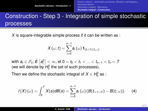
Construction - Step 3 - Integration of simple stochasticprocesses
X is square-integrable simple process if it can be written as :
X (ω, t) =n−1∑i=0
ai (ω) 1(ti<t≤ti+1)
with ai ∈ Fti , IE[a2
i
]<∞, et 0 = t0 < t1 < ... < tn−1 < tn = T
(we will denote by H20 the set of such processes).
Then we define the stochastic integral of X ∈ H20 as :
I (X ) (ω) =
∫ T
0X (s)dB(s) =
n−1∑i=0
ai (ω) (B(ti+1, ω)− B(ti ;ω)). (4)
C. Azizieh VUB Stochastic calculus : introduction

70/91
Stochastic calculus – Introduction – I
Known notions : stochastic processes, filtration, martingales,...Brownian MotionStochastic integral - MotivationStochastic integral - Construction
Construction - Step 4 - Extension by density
X is a square-integrable process on (0,T) if :X is an adapted process
IE[∫ T
0 X 2(ω, s)ds]<∞.
The set of square-integrable adapted processes will be denoted byH2 = H2 [0,T ]
Mathematicians show that H2 is a closed vector subspace ofL2 (dP× dt) .
We will denote by H20 (0,T ) the set of simple square-integrable (cf.
preceding slide).
C. Azizieh VUB Stochastic calculus : introduction

71/91
Stochastic calculus – Introduction – I
Known notions : stochastic processes, filtration, martingales,...Brownian MotionStochastic integral - MotivationStochastic integral - Construction
Construction - Step 4 - Extension by density
We will now extend the definition for all square-integrable processesX ∈ H2. The key of this extension is Ito isometry
Lemma (Ito Isometry on H20 )
∀X ∈ H20 , we have
‖I (X )‖L2(dP) = ‖X‖L2(dP×dt)
In other words :
IE((I(X ))2) = IE(
∫ T
0X 2(s)ds).
C. Azizieh VUB Stochastic calculus : introduction

72/91
Stochastic calculus – Introduction – I
Known notions : stochastic processes, filtration, martingales,...Brownian MotionStochastic integral - MotivationStochastic integral - Construction
Construction - Step 4 - Extension by densityProof of Ito isometryWe first calculate ‖X‖2
L2(dP×dt) .
X is a simple process, hence can be written in the form :
X (ω, t) =n−1∑i=0
ai (ω)1(ti<t≤ti+1)
with ai ∈ Fti , IE[a2
i
]<∞ and 0 = t0 < t1 < ... < tn = T
Let us take the square of X :
X 2 (ω, t) =n−1∑i=0
a2i (ω) 1(ti<t≤ti+1)
such that :
IE[∫ T
0 X 2 (ω, t) dt]
=n−1∑i=0
IE[a2
i
](ti+1 − ti ) .
C. Azizieh VUB Stochastic calculus : introduction

73/91
Stochastic calculus – Introduction – I
Known notions : stochastic processes, filtration, martingales,...Brownian MotionStochastic integral - MotivationStochastic integral - Construction
Construction - Etape 4 - Extension by densityLet us compute now ‖I (X )‖2
L2(dP) :
IE[I (X )2
]= IE
(n−1∑i=0
ai (ω)(Bti+1 − Bti
))2=
n−1∑i=0
IE[a2
i(Bti+1 − Bti
)2]
as the double products have a zero expectation. Then, as Bti+1 − Bti is
independent of ai ∈ Fti , we have :
IE[I (X )2
]=
n−1∑i=0
IE[a2
i
](ti+1 − ti ) .
C. Azizieh VUB Stochastic calculus : introduction

74/91
Stochastic calculus – Introduction – I
Known notions : stochastic processes, filtration, martingales,...Brownian MotionStochastic integral - MotivationStochastic integral - Construction
Construction - Step 4 - Extension by density
We will now extend by density the stochastic integral to the set ofsquare integrable processes. We will use the following result :
Lemma (density of H20 in H2)
For each process X ∈ H2, there exists a sequence Xn with Xn ∈ H20
such that
‖X − Xn‖2L2(dP×dt) = IE
[∫ T
0(X (s)− Xn(s))2ds
]−→ 0
for n −→∞.
C. Azizieh VUB Stochastic calculus : introduction

75/91
Stochastic calculus – Introduction – I
Known notions : stochastic processes, filtration, martingales,...Brownian MotionStochastic integral - MotivationStochastic integral - Construction
Ito integral - Construction - Step 4- Extension bydensity
Consequence of the Ito isometry and the density resultFor each simple process of the sequence, we can define itsstochastic integral : I(Xn) =
∫ T0 Xn(s)dB(s)
The idea is to define I (X ) for a general process X (notnecessarily simple) as the limit of the sequence I (Xn)n in L2 :
I (X )def= lim
n→∞(I (Xn))
where I (X ) ∈ L2 (dP) and the convergence is such that
‖I (X )− I (Xn)‖L2(dP) → 0.
C. Azizieh VUB Stochastic calculus : introduction

76/91
Stochastic calculus – Introduction – I
Known notions : stochastic processes, filtration, martingales,...Brownian MotionStochastic integral - MotivationStochastic integral - Construction
Construction - Step 4 - Extension by density
Let us check that the stochastic integral is well defined 1, i.e. that (1)the limit of the sequence I(Xn) exists and (2) does not depend on theconsidered sequence Xn tending to X :
(1) ‖X − Xn‖L2(dP×dt) → 0 implies that (I (Xn)) converges in L2 (dP) :
Indeed, the convergence of the sequence (Xn) in L2 (dP× dt) implies thatthis is a Cauchy sequence in L2 (dP× dt), which thanks to the Ito isometry,implies that (I (Xn)) is also a Cauchy sequence L2 (dP) .
As L2 (dP) is a complete metric space (convergence of Cauchy sequencestowards limits belonging to the space), the Cauchy sequence (I (Xn))converges to an element of L2 (dP), that we denote by I(X ).
1. The argument developed here is classical in functional analysisC. Azizieh VUB Stochastic calculus : introduction

77/91
Stochastic calculus – Introduction – I
Known notions : stochastic processes, filtration, martingales,...Brownian MotionStochastic integral - MotivationStochastic integral - Construction
Construction - Step 4 - Extension by density
(2) Is I(X ) well defined ? i.e. for another choice of the sequence (X ′n)nconverging to X :
‖X − X ′n‖L2(dP×dt) → 0,
does the new sequence I (X ′n) converges to the same limit in L2 (dP)as the initial sequence I (Xn) ?
The answer is yes, since ‖Xn − X ′n‖L2(dP×dt) → 0 thanks to the triangleinequality, and Ito isometry implies that :
‖I (Xn)− I (X ′n)‖L2(dP) → 0.
C. Azizieh VUB Stochastic calculus : introduction

78/91
Stochastic calculus – Introduction – I
Known notions : stochastic processes, filtration, martingales,...Brownian MotionStochastic integral - MotivationStochastic integral - Construction
Ito integral - Ito isometry
Now, we will show that when extended by density to the whole spaceH2, Ito integral is still an isometry :
Theorem (Ito isometry in H2 (0,T ))
For X ∈ H2 [0,T ], we have that
‖I (X )‖L2(dP) = ‖X‖L2(dP×dt) .
In other words,
IE
(∫ T
0X (s)dB(s)
)2 = IE
[∫ T
0X 2(s)ds
]
C. Azizieh VUB Stochastic calculus : introduction

79/91
Stochastic calculus – Introduction – I
Known notions : stochastic processes, filtration, martingales,...Brownian MotionStochastic integral - MotivationStochastic integral - Construction
Ito integral - Ito isometryProofFirst, we chose (Xn)n ∈ H2
0 such that
‖Xn − X‖L2(dP×dt) → 0 for n→∞.
The triangle inequality for the L2 (dP× dt) norm implies :
‖Xn‖L2(dP×dt) → ‖X‖L2(dP×dt) .
Similarly, since (I (Xn))nL2(dP)−→ I (X ),
‖I (Xn)‖L2(dP) → ‖I (X )‖L2(dP) .
But we know that on H20 , Ito isometry holds :
‖I (Xn)‖L2(dP) = ‖Xn‖L2(dP×dt) ∀n,
and the uniqueness of the limit completes the proof. C. Azizieh VUB Stochastic calculus : introduction
80/91
Stochastic calculus – Introduction – I
Known notions : stochastic processes, filtration, martingales,...Brownian MotionStochastic integral - MotivationStochastic integral - Construction
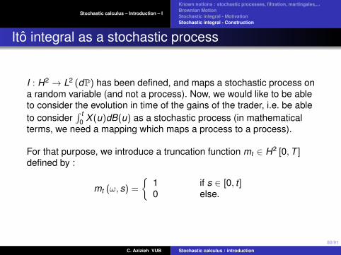
Ito integral as a stochastic process
I : H2 → L2 (dP) has been defined, and maps a stochastic process ona random variable (and not a process). Now, we would like to be ableto consider the evolution in time of the gains of the trader, i.e. be ableto consider
∫ t0 X (u)dB(u) as a stochastic process (in mathematical
terms, we need a mapping which maps a process to a process).
For that purpose, we introduce a truncation function mt ∈ H2 [0,T ]defined by :
mt (ω, s) =
1 if s ∈ [0, t ]0 else.
C. Azizieh VUB Stochastic calculus : introduction
81/91
Stochastic calculus – Introduction – I
Known notions : stochastic processes, filtration, martingales,...Brownian MotionStochastic integral - MotivationStochastic integral - Construction
Ito integral as a stochastic process
For X ∈ H2 [0,T ] , the product mtX ∈ H2 [0,T ] ∀t ∈ [0,T ], henceI (mtX ) =
∫ T0 mt (u)X (u)dB(u) is a well defined element of L2 (dP)
One can show that we can construct a continuous martingale Mt suchthat ∀t ∈ [0,T ], we have
P (Mt = I (mtX )) = 1.
The process Mt , t ∈ [0,T ] is then the Ito integral considered as aprocess.
C. Azizieh VUB Stochastic calculus : introduction

82/91
Stochastic calculus – Introduction – I
Known notions : stochastic processes, filtration, martingales,...Brownian MotionStochastic integral - MotivationStochastic integral - Construction
Ito integral as a stochastic process
Theorem (Ito integral as martingales)
for all X ∈ H2 [0,T ], there exists a process Mt , t ∈ [0,T ] which is acontinuous martingale w.r.t. the standard Brownian filtration (Ft )tsuch that the event :
ω : Mt (ω) = I (mtX ) (ω)
has a probability 1 for all t ∈ [0,T ] .
Proof : [Steele, pg 83-84, thm 6.2]
C. Azizieh VUB Stochastic calculus : introduction

83/91
Stochastic calculus – Introduction – I
Known notions : stochastic processes, filtration, martingales,...Brownian MotionStochastic integral - MotivationStochastic integral - Construction
Ito integral as a stochastic process
The integral sign : notationfor all X ∈ H2 [0,T ] and if Mt : 0 ≤ t ≤ T is a continuous martingalesuch that
P [Mt = I (mtX )] = 1 for all 0 ≤ t ≤ T ,
we write :
Mt (ω) =∫ t
0 X (ω, s) dBs ∀ 0 ≤ t ≤ T∫ t0 X (ω, s) dBs is a notation for what is well defined in the left-hand
side of the equation.
C. Azizieh VUB Stochastic calculus : introduction

84/91
Stochastic calculus – Introduction – I
Known notions : stochastic processes, filtration, martingales,...Brownian MotionStochastic integral - MotivationStochastic integral - Construction
Ito integral as a stochastic process
But the notation is well chosen since
X ∈ H2 =⇒ IE
(∫ t
0X (ω, s) dBs
)2 = IE
[∫ t
0X 2 (ω, s) ds
]∀t ∈ [0,T ] .
Moreover, we have the following result :
Proposition
for all 0 ≤ s ≤ t and for all b ∈ H2, we have
IE
(∫ t
sb (ω,u) dBu
)2
|Fs
= IE
[∫ t
sb (ω,u)2 du |Fs
]. (5)
C. Azizieh VUB Stochastic calculus : introduction

85/91
Stochastic calculus – Introduction – I
Known notions : stochastic processes, filtration, martingales,...Brownian MotionStochastic integral - MotivationStochastic integral - Construction
Ito integral as a stochastic process
ProofInequality (5) is equivalent to ∀A ∈ Fs :
IE[1A
(∫ ts b (ω,u) dBu
)2]
= IE[1A∫ t
s b2 (ω,u) du].
This is true by Theorem 1.4 on slide 78 for the modified integrand :
∧b (ω,u) =
0 u ∈ [0, s) ∪ (t ,T ]1Ab (ω,u) u ∈ [s, t ]
C. Azizieh VUB Stochastic calculus : introduction

86/91
Stochastic calculus – Introduction – I
Known notions : stochastic processes, filtration, martingales,...Brownian MotionStochastic integral - MotivationStochastic integral - Construction
Riemann’s representation
Theorem
For all f : R→ R continuous, if we consider the partition of [0,T ]given by ti = i T
n with 0 ≤ i ≤ n, we have :
limn→∞
n∑i=1
f(Bti−1
) (Bti − Bti−1
)=
∫ T
0f (Bs) dBs (6)
where the limit is taken in the sense of the convergence in probability.
C. Azizieh VUB Stochastic calculus : introduction

87/91
Stochastic calculus – Introduction – I
Known notions : stochastic processes, filtration, martingales,...Brownian MotionStochastic integral - MotivationStochastic integral - Construction
Stochastic integral : explicit calculation
In some cases, this integral can be explicitly computed from thedefinition.
Example :∫ t
0 Bs dBs =?
If we denote ∆iB := Bti − Bti−1 and ∆i t := ti − ti−1, we have :∑i
Bti−1
(∆iB
)=
∑i
(Bti−1Bti − B2
ti−1
)=
12
∑i
[(B2
ti − B2ti−1
)−(Bti − Bti−1
)2]
=12(B2
t − B20)− 1
2
∑i
(∆iB
)2=
12
B2t −
12
∑i
(∆iB
)2,
C. Azizieh VUB Stochastic calculus : introduction

88/91
Stochastic calculus – Introduction – I
Known notions : stochastic processes, filtration, martingales,...Brownian MotionStochastic integral - MotivationStochastic integral - Construction
Stochastic integral : explicit calculation
We have seen that ∑i
(∆iB
)2 → t
in L2. We then get : ∫ t
0Bs dBs =
12
B2t −
12
t .
Remark :We just saw that ”(∆iB)2 behaves like ∆i t” i.e., formally :
(dBt )2 = dt
C. Azizieh VUB Stochastic calculus : introduction

89/91
Stochastic calculus – Introduction – I
Known notions : stochastic processes, filtration, martingales,...Brownian MotionStochastic integral - MotivationStochastic integral - Construction
Riemann’s representationProposition (Gaussian integrals)
Let f ∈ C[0,T ] (a deterministic function), then the process defined by
Xt =
∫ t
0f (s)dBs for all t ∈ [0,T ]
is a Gaussian process of zero mean with indepent increments and withcovariance function
cov(Xs,Xt ) =
∫ s∧t
0f 2(u)du.
Moreover, if we consider the partition of [0,T ] given by ti = iTn for 0 ≤ i ≤ n
and t∗i ∈ [ti−1, ti ], then
limn→∞
n∑i=1
f (t∗i )(Bti − Bti−1
)=
∫ T
0f (s)dBs,
where the limit is taken in the sense of the convergence in probability.
C. Azizieh VUB Stochastic calculus : introduction

90/91
Stochastic calculus – Introduction – I
Known notions : stochastic processes, filtration, martingales,...Brownian MotionStochastic integral - MotivationStochastic integral - Construction
Interpretation trajectory by trajectory of the Ito integral
Theorem (Interpretation trajectory by trajectory of the Ito integralon H2)
If f ∈ H2 is bounded and if ν is a stopping time such that f (ω, s) = 0for almost all ω ∈ ω : s ≤ ν,then
Xt (ω) =∫ t
0 f (ω, s) dBs = 0
for almost all ω ∈ ω : t ≤ ν .
C. Azizieh VUB Stochastic calculus : introduction

91/91
Stochastic calculus – Introduction – I
Known notions : stochastic processes, filtration, martingales,...Brownian MotionStochastic integral - MotivationStochastic integral - Construction
Interpretation trajectory by trajectory of the Ito integral
Theorem (Persistence of the identity on H2)
If f and g ∈ H2 and if ν is a stopping time such that f (ω, s) = g (ω, s)for almost all ω ∈ ω : s ≤ ν,then the integrals
Xt (ω) =∫ t
0 f (ω, s) dBs and Yt (ω) =∫ t
0 g (ω, s) dBs
are equal for almost all ω ∈ ω : t ≤ ν .
C. Azizieh VUB Stochastic calculus : introduction