Mathematical Biosciences 223 (2010) 32–46

Contents lists available at ScienceDirect

Mathematical Biosciences

journal homepage: www.elsevier .com/locate /mbs

Stochastic eco-epidemiological model of dengue disease transmissionby Aedes aegypti mosquito

M. Otero *, H.G. SolariDepartamento de Física, Facultad de Ciencias Exactas y Naturales, Universidad de Buenos Aires, Pabellón 1 Ciudad Universitaria, 1428 Ciudad Autónoma de Buenos Aires, Argentina

a r t i c l e i n f o a b s t r a c t

Article history:Received 9 January 2009Received in revised form 9 October 2009Accepted 15 October 2009Available online 25 October 2009

Keywords:Eco-epidemiologyAedes aegyptiStochastic modelsDengue

0025-5564/$ - see front matter � 2009 Elsevier Inc. Adoi:10.1016/j.mbs.2009.10.005

* Corresponding author.E-mail addresses: mjotero@df.uba.ar (M. Otero), so

We present a stochastic dynamical model for the transmission of dengue that takes into account seasonaland spatial dynamics of the vector Aedes aegypti. It describes disease dynamics triggered by the arrival ofinfected people in a city. We show that the probability of an epidemic outbreak depends on seasonal var-iation in temperature and on the availability of breeding sites. We also show that the arrival date of aninfected human in a susceptible population dramatically affects the distribution of the final size of epi-demics and that early outbreaks have a low probability. However, early outbreaks are likely to producelarge epidemics because they have a longer time to evolve before the winter extinction of vectors. Ourmodel could be used to estimate the risk and final size of epidemic outbreaks in regions with seasonalclimatic variations.

� 2009 Elsevier Inc. All rights reserved.

1. Introduction

Arboviruses is a shortened name given to arthropod-borneviruses from various families which are transmitted by arthropods.Some Arboviruses are able to cause re-emergent diseases such asSt. Louis Encephalitis, Chikungunya, Dengue, Ross River disease,West Nile, Yellow Fever, Equine Encephalitis, etc. [1]. Arthropodsare able to transmit the virus upon biting the host, allowing thevirus to enter the host’s bloodstream. The virus replicates in thevector but usually does not harm it. In the mosquito-borne dis-eases, the virus establishes a persistent infection in the mosquitosalivary glands and there is sufficient virus in the saliva to infectanother host during feeding. Each arbovirus usually grows onlyin a limited number of mosquito species. The work presented inthis article is focused on mosquito-borne diseases (mainly denguefever) transmitted by Aedes aegypti. This is one of the most efficientmosquito vectors for arboviruses, because it is highly anthropo-philic, thrives in close proximity to humans and often lives indoors.

Dengue is spread only by adult females, which require blood tocomplete oogenesis. During the blood meal the female ingests den-gue viruses from an infectious human. The viruses develop withinthe mosquito and are re-injected in later blood meals into theblood stream of susceptible humans. Dengue is an acute febrile vir-al disease (with four serotypes of flaviviruses DEN1;DEN2;DEN3and DEN4) which presents headaches, bone, joint and muscularpains, rash and leukopenia as symptoms. Dengue epidemics werereported throughout the 19th and 20th centuries in the Americas,

ll rights reserved.

lari@df.uba.ar (H.G. Solari).

southern Europe, northern Africa, the eastern Mediterranean, Asia,Australia and on various islands in the Indian Ocean, Central Pacificand Caribbean [2].

The history of dengue in Argentina began as early as in 1916when an epidemic affected the cities of Concordia and Paraná. In1947 the Pan American Health Organization (PHO) led a continen-tal mosquito eradication program and by 1967 the mosquito wasconsidered to be eradicated in Argentina. The mosquito was de-tected again in 1986 and since 1997 several epidemic outbreakstook place in the northwestern and northeastern regions of thecountry. A brief history of dengue epidemics in Argentina is foundin Appendix A.

Nowadays A. aegypti is a permanent inhabitant of the city ofBuenos Aires [3–5]. Every summer there is a potential risk of den-gue virus transmission because of the arrival of viremic peoplefrom Bolivia, Paraguay, Brazil and other endemic countries. How-ever, no autochthonous cases of the disease have been detecteduntil present [5], but in the last years some clinical studies con-firmed dengue infection in people arriving from neighboring ende-mic countries [6]. Therefore, the development of mathematicalmodels which permit the estimation of the probability of an epi-demic outbreak and its final size has become a matter of sanitarynecessity.

The first model of dengue was performed by Newton and Reiterin 1992 [7]. They developed a deterministic model in which thepopulations of hosts and vectors were divided into subpopulationsrepresenting disease status and the flow between subpopulationswas described by differential equations. Several deterministicmodels have been developed taking into account different possibleaspects of the disease: constant human population and variable

M. Otero, H.G. Solari / Mathematical Biosciences 223 (2010) 32–46 33

vector population [8], variable human population size [9], verticaland mechanical transmission in the vector population [10], season-ally varying parameters and presence of two simultaneous dengueserotypes [11], age structure in the human population [12] andpresence of two serotypes of dengue at separated intervals of time[13]. In addition, in 2006 Tran and Raffy proposed a spatial andtemporal dynamical model based on diffusion equations using re-mote-sensing data [14].

There are also other approaches. Focks et al. developed a sto-chastic model that describes the daily dynamics of dengue virustransmission in an urban environment based on the simulationof a human population growing in response to country- and age-specific birth and death rates [15]. Santos et al. developed a period-ically forced two-dimensional cellular automata model that de-scribes complex features of the disease taking into accountexternal seasonality (rainfall) and human and mosquito mobility[16].

Our proposal in this article is the third in a series of minimaliststochastic models. The first describes the seasonal dynamics of A.aegypti populations in a homogeneous environment [17]. The sec-ond one describes the A. aegypti dispersal driven by the availabilityof oviposition sites in an urban environment [18]. This new modeltakes into account the seasonal and spatial dynamics of the vectorsand describes the disease dynamics triggered by the arrival of vire-mic people in a city.

Our main goal is the development of a mathematical tool thatallows the study of different epidemic scenarios in an urban envi-ronment, the estimation of the epidemic risk and the study of thegrowth and final size of an epidemic outbreak due to the spatialdynamics of the vector. A particular aim of the work is the estima-tion of dengue epidemic risk in the city of Buenos Aires, Argentina.

Populations of hosts (Humans) and vectors (A. aegypti) were di-vided into subpopulations representing disease status: susceptible(S), exposed (E) and infectious (I) for adult female vectors, and sus-ceptible (S), exposed (E), infectious (I) and removed (R) for the hu-man population. The population of adult male mosquitoes is nottaken into account explicitly and we consider that, on average,one half of the emerging adults are females [19]. Three kinds of fe-males were considered: adult females in their first gonotrophic cy-cle (A1 females), females in subsequent gonotrophic cycles (A2females) and flyers (F), which are the adult females that have al-ready finished their gonotrophic cycles and fly in order to deposittheir eggs.

The following sections will describe the populations andevents of the stochastic transmission model (Section 2), themathematical description of the stochastic model (Section 3),the parameters, initial values and boundary conditions (Section4), results and discussion (Section 5), the transcription of thedengue model into a yellow fever model, the choice of dengueparameters as well as some minimal computations in the valida-tion direction (Section 6), and finally, summary and conclusions(Section 7).

2. Populations and events of the stochastic transmission model

2.1. Populations of the stochastic process

We consider a two-dimensional space as a mesh of squaredpatches where the dynamics of the immature stages of the mosquitoand the evolution of the disease take place, and where only Flyers canfly from one patch to the next according to a diffusion-like process.We take into account that during the gonotrophic cycles the mos-quito dispersal is negligible, and once the gonotrophic cycle endsthe female begins to fly, becoming a Flyer in search of ovipositionsites. A detailed explanation of the dispersal model has been already

presented [18]. In the present work, host movement was not takeninto account.

The patch coordinates are given by two indices, i and j, corre-sponding to the row and column in the mesh. If Xk is a subpopula-tion in the stage k, then Xkði; jÞ is the Xk subpopulation in the patchof coordinates ði; jÞ.

The transmission of only one serotype of virus was considered,and mechanical transmission (i.e., without amplification of thevirus in the vector) was not taken into account. The populationsof both hosts (Humans) and vectors (A. aegypti) were divided intosubpopulations representing disease status: S.E.I for the vectorsand S.E.I.R for the human population.

Ten different subpopulations for the mosquito were taken intoaccount: three immature subpopulations (eggs Eði;jÞ, larvae Lði;jÞand pupae Pði;jÞ), and seven adult subpopulations (female adultsnot having laid eggs A1ði;jÞ, susceptible flyers Fsði;jÞ, exposed flyersFeði;jÞ, infectious flyers Fiði;jÞ and female adults having laid eggsaccording to their disease status: susceptible A2sði;jÞ, exposedA2eði;jÞ and infectious A2iði;jÞ).

A1ði;jÞ are always susceptible because we neglect the verticaltransmission of the virus. After a blood meal, A1ði;jÞ become eithersusceptible Fsði;jÞ or exposed Feði;jÞ, depending on the disease statusof the host. If the host is infectious, A1ði;jÞ become Feði;jÞ but if thehost is not infectious, then A1ði;jÞ become Fsði;jÞ.

The human population Nhði;jÞ was split into four different sub-populations according to the disease status: susceptible humansHsði;jÞ, exposed humans Heði;jÞ, infectious humans Hiði;jÞ and removedhumans Hrði;jÞ.

The evolution of all the 14 subpopulations is affected by 38 dif-ferent possible events. Events occur at rates that depend on sub-population values and some of them also on temperature, whichis a function of time since it changes over the course of the yearseasonally [17,18]. Hence, the dependence on temperature intro-duces a time dependence in the event rates. A brief descriptionof the temperature model is presented in Appendix B.

2.2. Events related to immature stages

Pre-imaginal stages of domestic A. aegypti develop in artificialcontainers of small volume such as buckets, jars, flasks, bottlesand flower vases [20]. The natural regulation of A. aegypti popula-tions is due to intra-specific competition for food and other re-sources in the larval stage. This regulation was incorporated intothe model as a density-dependent transition probability whichintroduces the necessary non-linearities that prevent a Malthusiangrowth of the population. This effect was incorporated as a nonlin-ear correction to the temperature-dependent larval mortality.

Then, larval mortality can be written as:

x3ðLði;jÞÞ ¼ mlLði;jÞ þ aLði;jÞ � ðLði;jÞ � 1Þ ð1Þ

where the value of a can be further decomposed as

a ¼ a0=BSði;jÞ ð2Þ

with a0 associated with the carrying capacity of one (standardized)breeding site and BSði;jÞ being the density of breeding sites in the ði; jÞpatch [17,18].

Table 1 summarizes the events and rates related to immaturestages of the mosquito during their first gonotrophic cycle. Theconstruction of the transition rates and the choice of model param-eters related to the mosquito biology, such as mortality of eggs(me), hatching rate (elr), mortality of larvae (ml), density-depen-dent mortality of larvae (a), pupation rate (lpr), mortality of pupae(mp), pupae into adults development coefficient (par), and emer-gence factor (ef), have been previously described in detail [17,18].

Table 1Event type, effects on the populations and transition rates for the developmentalmodel. The coefficients are me: mortality of eggs; elr: hatching rate; ml: mortality oflarvae; a: density-dependent mortality of larvae; lpr: pupation rate; mp: mortality ofpupae; par: pupae into adults development coefficient; ef: emergence factor. Thevalues of the coefficients are available in Section 4.

Event Effect Transition rate

(1) Egg death Eði;jÞ ! Eði;jÞ � 1 w1 ¼ me � Eði;jÞ

(2) Egg hatching Eði;jÞ ! Eði;jÞ � 1 w2 ¼ elr � Eði;jÞLði;jÞ ! Lði;jÞ þ 1

(3) Larval death Lði;jÞ ! Lði;jÞ � 1 w3 ¼ ml � Lði;jÞ þ a � Lði;jÞ � ðLði;jÞ � 1Þ

(4) Pupation Lði;jÞ ! Lði;jÞ � 1 w4 ¼ lpr � Lði;jÞPði;jÞ ! Pði;jÞ þ 1

(5) Pupal death Pði;jÞ ! Pði;jÞ � 1 w5 ¼ ðmpþ par � ð1� ðef=2ÞÞÞ � Pði;jÞ

(6) Adult emergence Pði;jÞ ! Pði;jÞ � 1 w6 ¼ par � ðef=2Þ � Pði;jÞA1ði;jÞ ! A1ði;jÞ þ 1

34 M. Otero, H.G. Solari / Mathematical Biosciences 223 (2010) 32–46

2.3. Local events related to the adult stage

As we have already explained in Section 1, A. aegypti females re-quire blood to complete their gonotrophic cycles. In this process,the female may ingest viruses with the blood meal from an infec-tious human during its Viremic Period (VP). The viruses developwithin the mosquito during the Extrinsic Incubation Period (EIP)and are then re-injected into the blood stream of a new susceptiblehuman in later blood meals. The virus in the exposed human devel-ops during the Intrinsic Incubation Period (IIP) and then begins tocirculate in the blood stream, making the human infectious. Theflow from susceptible to exposed subpopulations (in the vectorand the host) depends not only on the contact between vectorand host but also on the transmission probabilities of the virus:the transmission probability from host to vector (ahv) and thetransmission probability from vector to host (avh).

Local events related to the adult stage are shown in Tables 2–5.Table 2 summarizes the events and rates related to adults duringtheir first gonotrophic cycle and related to oviposition by flyersaccording to their disease status. Tables 3 and 4 summarize theevents and rates related to human contagion, A2 gonotrophic cy-cles and A2eði;jÞ and Feði;jÞ that become infectious. Table 5 summa-rizes the events and rates related to the death of A2 and F.

2.4. Events related to flyer dispersal

The development of A. aegypti requires resting sites, ovipositionsites, nectar and blood resources. Different levels of urbanization

Table 2Event type, effects on the subpopulations and transition rates for the developmental mod(number of daily cycles) for adult females in stages A1; ahv: transmission probability from hof eggs laid in an oviposition. The values of the coefficients are available in Section 4.

Event Effect

(7) Adults 1 death A1ði;jÞ ! A1ði;jÞ � 1

(8) I Gonotrophic cycle with virus exposure A1ði;jÞ ! A1ði;jÞ � 1Feði;jÞ ! Feði;jÞ þ 1

(9) I Gonotrophic cycle without virus exposure A1ði;jÞ ! A1ði;jÞ � 1Fsði;jÞ ! Fsði;jÞ þ 1

(10) Oviposition of susceptible flyers Eði;jÞ ! Eði;jÞ þ egnFsði;jÞ ! Fsði;jÞ � 1A2sði;jÞ ! A2sði;jÞ þ 1

(11) Oviposition of exposed flyers Eði;jÞ ! Eði;jÞ þ egnFeði;jÞ ! Feði;jÞ � 1A2eði;jÞ ! A2eði;jÞ þ 1

(12) Oviposition of infected flyers Eði;jÞ ! Eði;jÞ þ egn

Fiði;jÞ ! Fiði;jÞ � 1A2iði;jÞ ! A2iði;jÞ þ 1

might be associated with differences in the availability of these re-sources or the connectivity between patches with resources. Lessmosquito activity was observed in more urbanized areas withhigher density of apartments and/or human population density.In contrast, more activity was observed in less urbanized areaswith higher house density and/or closer to industrial sites [21].

One open question about A. aegypti dispersal is the motivationof the flight. In fact, some experimental results and observationalstudies show that A. aegypti dispersal is driven by the availabilityof oviposition sites [22–24]. According to these observations, weconsidered that only Fði;jÞ can fly from patch to patch in search ofoviposition sites. Flyer dispersal events correspond to event num-bers n from 26 to 31. The implementation of flyer dispersal hasbeen described previously [18].

The general rate of the dispersal event is given by:

wn ¼ b � Fði;jÞ ð3Þ

where n is the event number ðn ¼ 26;27; . . . ;31Þ; b is the dispersalcoefficient and Fði;jÞ is the Flyer population which can be susceptibleFsði;jÞ, exposed Feði;jÞ or infectious Fiði;jÞ.

The dispersal coefficient b can be written as

b ¼0 if the patches are disjoint

diff=d2ij if the patches have at least a common point

(

ð4Þ

where dij is the distance between the centers of the patches and diffis a diffusion-like coefficient so that dispersal is compatible with adiffusion-like process [18].

2.5. Events related to the human population

Table 6 summarizes the events and rates in which humans areinvolved. Human contagion has been already described in Table 4and the evolution of the disease in humans is described in Section2.3. The human population was fluctuating but balanced, meaningthat the birth coefficient was considered equal to the mortalitycoefficient (mh).

3. Mathematical description of the stochastic model

The evolution of the subpopulations is modelled by a state-dependent Poisson process [25,26] where the probability of thestate:

el. The coefficients are ma: mortality of adults; cycle1: gonotrophic cycle coefficientost to vector; ovrði;jÞ: oviposition rate by flyers in the (i, j) patch; egn: average number

Transition rate

w7 ¼ ma � A1ði;jÞ

w8 ¼ cycle1 � A1ði;jÞ � ðHiði;jÞ=Nhði;jÞÞ � ahv

w9 ¼ cycle1 � A1ði;jÞ � ðððNhði;jÞ � Hiði;jÞÞ=Nhði;jÞÞ þ ð1� ahvÞ � ðHiði;jÞ=Nhði;jÞÞÞ

w10 ¼ ovrði;jÞ � Fsði;jÞ

w11 ¼ ovrði;jÞ � Feði;jÞ

w12 ¼ ovrði;jÞ � Fiði;jÞ

Table 3Event type, effects on the subpopulations and transition rates for the developmental model. The coefficients are cycle2: gonotrophic cycle coefficient (number of daily cycles) foradult females in stages A2; ahv: transmission probability from host to vector. The values of the coefficients are available in Section 4.

Event Effect Transition rate

(13) II Gonotrophic cycle of susceptibleAdults 2 with virus exposure

A2sði;jÞ ! A2sði;jÞ � 1 w13 ¼ cycle2 � A2sði;jÞ � ðHiði;jÞ=Nhði;jÞÞ � ahv

Feði;jÞ ! Feði;jÞ þ 1

(14) II Gonotrophic cycle of susceptibleAdults 2 without virus exposure

A2sði;jÞ ! A1ði;jÞ � 1 w14 ¼ cycle2 � A2sði;jÞ � ðððNhði;jÞ � Hiði;jÞÞ=Nhði;jÞÞ þ ð1� ahvÞastðHiði;jÞ=Nhði;jÞÞÞ

Fsði;jÞ ! Fsði;jÞ þ 1

(15) II Gonotrophic cycle of exposed Adults 2 A2eði;jÞ ! A2eði;jÞ � 1 w15 ¼ cycle2 � A2eði;jÞFeði;jÞ ! Feði;jÞ þ 1

Table 4Event type, effects on the subpopulations and transition rates for the developmental model. The coefficients are cycle2: gonotrophic cycle coefficient (number of daily cycles) foradult females in stages A2; ovrði;jÞ: oviposition rate by flyers in the (i,j) patch; avh: transmission probability from vector to host; EIP: extrinsic incubation period. The values of thecoefficients are available in Section 4.

Event Effect Transition rate

(16) Exposed adults 2 becoming infectious A2eði;jÞ ! A2eði;jÞ � 1 w16 ¼ ð1=ðEIP � ð1=ovrði;jÞÞÞ�ÞA2eði;jÞA2iði;jÞ ! A2iði;jÞ þ 1

(17) Exposed flyers becoming infectious Feði;jÞ ! Feði;jÞ � 1 w17 ¼ ð1=ðEIP � ð1=ovrði;jÞÞÞ�ÞFeði;jÞFiði;jÞ ! Fiði;jÞ þ 1

(18) II Gonotrophic cycle of infectious Adults 2with human contagion

A2iði;jÞ ! A2iði;jÞ � 1 w18 ¼ cycle2 � A2iði;jÞ � ðHsði;jÞ=Nhði;jÞÞ � avh

Fiði;jÞ ! Fiði;jÞ þ 1Hsði;jÞ ! Hsði;jÞ � 1Heði;jÞ ! Heði;jÞ þ 1

(19) II Gonotrophic cycle of infectious Adults 2without human contagion

A2iði;jÞ ! A2iði;jÞ � 1 w19 ¼ cycle2 � A2iði;jÞ � ðððNhði;jÞ � Hsði;jÞÞ=Nhði;jÞÞ þ ð1� avhÞ � ðHsði;jÞ=Nhði;jÞÞÞ

Fiði;jÞ ! Fiði;jÞ þ 1

Table 5Event type, effects on the subpopulations and transition rates for the developmentalmodel. The coefficients are ma: adult mortality. The values of the coefficients areavailable in Section 4.

Event Effect Transition rate

(20) Susceptible flyer death Fsði;jÞ ! Fsði;jÞ � 1 w20 ¼ ma � Fsði;jÞ(21) Exposed flyer death Feði;jÞ ! Feði;jÞ � 1 w21 ¼ ma � Feði;jÞ(22) Infectious flyer death Fiði;jÞ ! Fiði;jÞ � 1 w22 ¼ ma � Fiði;jÞ(23) Susceptible adult 2 death A2sði;jÞ ! A2sði;jÞ � 1 w23 ¼ ma � A2sði;jÞ(24) Exposed adult 2 death A2eði;jÞ ! A2eði;jÞ � 1 w24 ¼ ma � A2eði;jÞ(25) Infectious adult 2 death A2iði;jÞ ! A2iði;jÞ � 1 w25 ¼ ma � A2iði;jÞ

M. Otero, H.G. Solari / Mathematical Biosciences 223 (2010) 32–46 35

ðE; L; P;A1;A2s;A2e;A2i; Fs; Fe; Fi;Hs;He;Hi:HrÞði;jÞ

evolves in time following a Kolmogorov forward equation that canbe constructed directly from the information collected in Tables 1–6

Table 6Event type, effects on the subpopulations and transition rates for the developmental mhuman mortality coefficient; IIP: intrinsic incubation period. The values of the coef

Event

(32) Birth of susceptible humans

(33) Death of susceptible humans

(34) Death of exposed humans

(35) Transformation from exposed to viremic

(36) Death of Infectious humans

(37) Removal of infectious humans

(38) Death of removed humans

odel.ficient

and in Eq. (4). Fig. 1 shows the subpopulations of vector populationsand the events which affect these populations collected in Tables 1–5 and Eq. (4). Fig. 2 shows the subpopulations of human populationsand the events which affect these populations collected in Tables 4and 6.

3.1. Deterministic rates approximation for the density-dependentMarkov process

We consider X is an integer vector having as entries the popula-tions under consideration, and ea;a ¼ 1 . . . j the events at whichthe populations change by a fixed amount Da in a Poisson processwith density-dependent rates. Then, a theorem by Kurtz andco-worker [25] allows us to rewrite the stochastic process as:

XðtÞ ¼ Xð0Þ þXja¼1

DaYZ t

0xaðXðsÞÞds

� �ð5Þ

The coefficients are mh: human mortality coefficient; VP: human viremic period; mh:s are available in Section 4.

Effect Transition rate

Hsði;jÞ ! Hsði;jÞ þ 1 w32 ¼ mh � Nhði;jÞ

Hsði;jÞ ! Hsði;jÞ � 1 w33 ¼ mh � Hsði;jÞ

Heði;jÞ ! Heði;jÞ � 1 w34 ¼ mh � Heði;jÞ

Heði;jÞ ! Heði;jÞ � 1 w35 ¼ ð1=IIPÞ � Heði;jÞHiði;jÞ ! Hiði;jÞ þ 1

Hiði;jÞ ! Hiði;jÞ � 1 w36 ¼ mh � Hiði;jÞ

Hiði;jÞ ! Hiði;jÞ � 1 w37 ¼ ð1=VPÞ � Hiði;jÞHrði;jÞ ! Hrði;jÞ þ 1

Hrði;jÞ ! Hrði;jÞ � 1 w38 ¼ mh � Hrði;jÞ

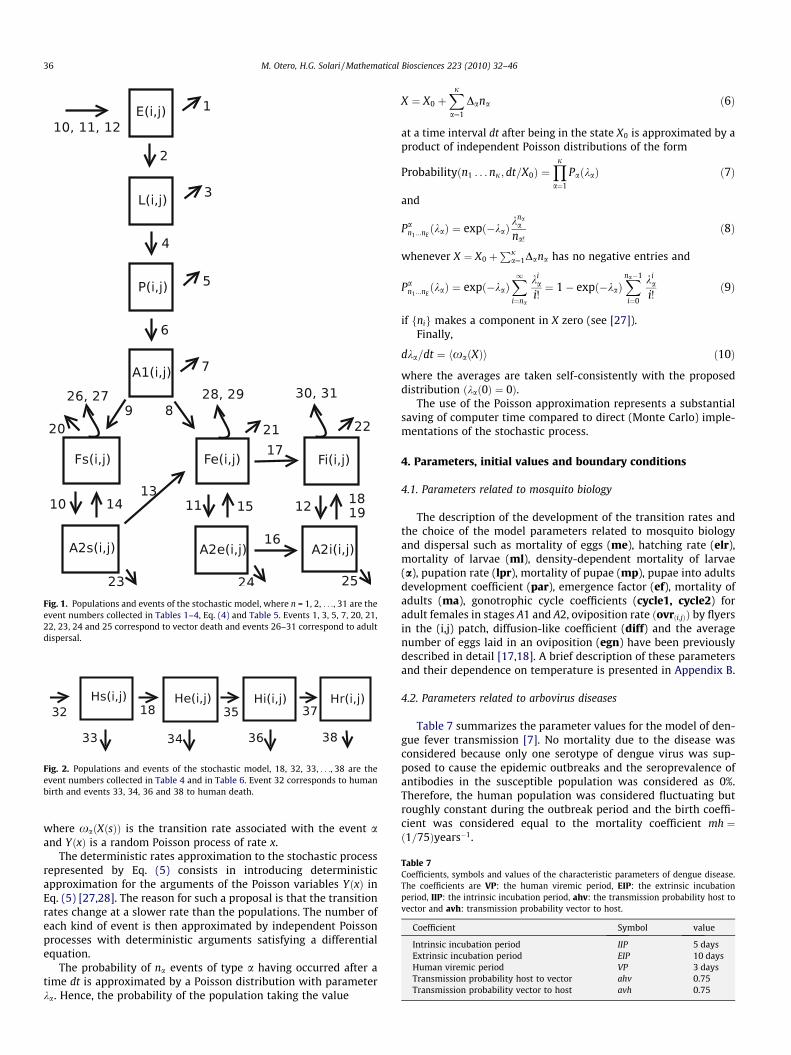
Fig. 1. Populations and events of the stochastic model, where n = 1, 2, . . ., 31 are theevent numbers collected in Tables 1–4, Eq. (4) and Table 5. Events 1, 3, 5, 7, 20, 21,22, 23, 24 and 25 correspond to vector death and events 26–31 correspond to adultdispersal.

Fig. 2. Populations and events of the stochastic model, 18, 32, 33, . . ., 38 are theevent numbers collected in Table 4 and in Table 6. Event 32 corresponds to humanbirth and events 33, 34, 36 and 38 to human death.

Table 7Coefficients, symbols and values of the characteristic parameters of dengue disease.The coefficients are VP: the human viremic period, EIP: the extrinsic incubationperiod, IIP: the intrinsic incubation period, ahv: the transmission probability host tovector and avh: transmission probability vector to host.

Coefficient Symbol value

Intrinsic incubation period IIP 5 daysExtrinsic incubation period EIP 10 daysHuman viremic period VP 3 daysTransmission probability host to vector ahv 0.75Transmission probability vector to host avh 0.75

36 M. Otero, H.G. Solari / Mathematical Biosciences 223 (2010) 32–46

where xaðXðsÞÞ is the transition rate associated with the event aand YðxÞ is a random Poisson process of rate x.

The deterministic rates approximation to the stochastic processrepresented by Eq. (5) consists in introducing deterministicapproximation for the arguments of the Poisson variables YðxÞ inEq. (5) [27,28]. The reason for such a proposal is that the transitionrates change at a slower rate than the populations. The number ofeach kind of event is then approximated by independent Poissonprocesses with deterministic arguments satisfying a differentialequation.

The probability of na events of type a having occurred after atime dt is approximated by a Poisson distribution with parameterka. Hence, the probability of the population taking the value

X ¼ X0 þXja¼1

Dana ð6Þ

at a time interval dt after being in the state X0 is approximated by aproduct of independent Poisson distributions of the form

Probabilityðn1 . . . nj; dt=X0Þ ¼Yja¼1

PaðkaÞ ð7Þ

and

Pan1 ...nE

ðkaÞ ¼ expð�kaÞknaa

na!

ð8Þ

whenever X ¼ X0 þPj

a¼1Dana has no negative entries and

Pan1 ...nE

ðkaÞ ¼ expð�kaÞX1i¼na

kia

i!¼ 1� expð�kaÞ

Xna�1

i¼0

kia

i!ð9Þ

if fnig makes a component in X zero (see [27]).Finally,

dka=dt ¼ hxaðXÞi ð10Þ

where the averages are taken self-consistently with the proposeddistribution ðkað0Þ ¼ 0Þ.

The use of the Poisson approximation represents a substantialsaving of computer time compared to direct (Monte Carlo) imple-mentations of the stochastic process.

4. Parameters, initial values and boundary conditions

4.1. Parameters related to mosquito biology

The description of the development of the transition rates andthe choice of the model parameters related to mosquito biologyand dispersal such as mortality of eggs (me), hatching rate (elr),mortality of larvae (ml), density-dependent mortality of larvae(a), pupation rate (lpr), mortality of pupae (mp), pupae into adultsdevelopment coefficient (par), emergence factor (ef), mortality ofadults (ma), gonotrophic cycle coefficients (cycle1, cycle2) foradult females in stages A1 and A2, oviposition rate ðovrði;jÞÞ by flyersin the (i,j) patch, diffusion-like coefficient (diff) and the averagenumber of eggs laid in an oviposition (egn) have been previouslydescribed in detail [17,18]. A brief description of these parametersand their dependence on temperature is presented in Appendix B.

4.2. Parameters related to arbovirus diseases

Table 7 summarizes the parameter values for the model of den-gue fever transmission [7]. No mortality due to the disease wasconsidered because only one serotype of dengue virus was sup-posed to cause the epidemic outbreaks and the seroprevalence ofantibodies in the susceptible population was considered as 0%.Therefore, the human population was considered fluctuating butroughly constant during the outbreak period and the birth coeffi-cient was considered equal to the mortality coefficient mh ¼ð1=75Þyears�1.

M. Otero, H.G. Solari / Mathematical Biosciences 223 (2010) 32–46 37

4.3. Initial values and boundary conditions

Studies performed in the city of Buenos Aires [5,29] have shown aparticular spatial distribution of the mosquito and suggest that theextinction of adults and all aquatic forms of the mosquito are com-mon in localized areas of the city, being the egg stage the only onethat can survive the winter period. According to these observations,we chose as initial time July 1st, ran the model with different initialegg population values and observed no significant differences in anypopulation numbers provided the mosquito survived until the fol-lowing favorable season (spring–summer) [17,18]. These resultsshow a very strong regulatory capability of the environment. Thecarrying capacity of the environment, reflected by the Breeding Siteparameter ðBSÞ, regulates the mosquito populations, which show lit-tle to no memory of the population situation 1 year before. There-fore, we used 10,000 eggs/ha as initial value for the mosquitopopulations and considered 1 year as transient period.

Many quarters suitable for the mosquito development have apopulation density lower than the population density of the city(146.3 inhab./ha). Then, we considered as mean population density100 inhab./ha according to the population densities of the quarterswith high mosquito abundance.

The spatial boundary condition takes into account that theprobability of the flyers Fði;jÞ flying away from the region understudy was considered equal to the probability of flying into thatregion, which means a zero average derivative condition. Thisassumes that the patch is just part of a larger region with the samefavorable conditions for the mosquitoes.

5. Results and discussion

5.1. Effect of the date of arrival of one exposed human in the final sizeof the epidemics

Fig. 3 shows the frequency of the final size of epidemics as a func-tion of the date of arrival of one exposed human in the susceptible

Fig. 3. Histograms of final size of epidemics vs. date of arrival of one exposed human in thof 100 susceptible humans/patch.

human population. By final size of epidemics we understand thetotal number of susceptible humans who were infected during theepidemic outbreak. We performed the simulations using a grid with13 � 13 patches and with a density of breeding sites of 200 BS/patch.We started with 100 susceptible humans and 10,000 mosquito eggsin every patch July 1st and we ran the simulations for 2 years. Theseasonal variation of temperature was calculated by using Eq. (16)(see Appendix B). Only the second year of each simulation was ana-lyzed since the first year was considered as transient (see Section4.3). This procedure was repeated 100 times for 12 different datesof arrival of one exposed human in the susceptible human popula-tion in the central patch of the grid during the second year of the sim-ulation. Histograms of the final size of epidemics were constructedusing a bin size of 1000.

Fig. 3 shows that no epidemic outbreaks take place during thewinter season and that the final size distribution is bimodal (i.e.,either no or only a few individuals are infected or else a fairly largeproportion of the susceptible population is infected, such as instandard Markovian SIR epidemic models) [26]. Fig. 3 also showsthat the date of arrival of the exposed human affects not only theshape but also the center of the distribution.

In order to see more clearly the details of the histograms, Fig. 4shows the histograms of non-zero final size of epidemics for fourdifferent dates of arrival of the exposed human: November 1st,December 1st, January 1st and February 1st. This is, the relativefrequency of an epidemic according to the size (binned) condi-tioned to be a non-zero epidemic. The analysis of the probabilityof no-development of an epidemic outbreak is discussed in Section5.2.

Fig. 4 clearly shows that the date of arrival of the exposed humandramatically affects the distribution of the final size of epidemics. Ifthe exposed human is incorporated into the susceptible populationon November 1st, the frequency of development of epidemicoutbreaks is low but instead the maximum final size is very highreaching almost 62% of the initial susceptible population. That corre-sponds to a scenario in which the probability of an epidemic

e susceptible population for simulations with 200 BS/patch and an initial population

0 2000 4000 6000 8000 10000 120000

0.10.20.30.40.50.6

November

0 2000 4000 6000 8000 10000 120000

0.050.1

0.150.2

0.25

December

0 2000 4000 6000 8000 10000 120000

0.050.1

0.150.2

January

0 2000 4000 6000 8000 10000 12000Final Size of Epidemic

00.05

0.10.150.2

0.25

February

Fig. 4. Relative frequency of non-zero final size of epidemics for different dates of arrival of the exposed human in the susceptible population for simulations with 200 BS/patch, an initial population of 100 susceptible humans/patch and dates of arrival of the exposed human: November 1st, December 1st, January 1st and February 1st.

38 M. Otero, H.G. Solari / Mathematical Biosciences 223 (2010) 32–46

outbreak is low but in case of an outbreak the consequences are ofsanitary emergency. By comparing the four histograms it can be seenthat the later the date of arrival of the exposed human during thesummer season, the lower the centers of the final size distribution.In order to understand the underlying processes that determine thisbehavior, we compared the temporal dynamics of the infectiouspopulation with the temporal dynamics of the mosquitoes (Fig. 5).

Fig. 5A shows the evolution of the infectious human populationunder the conditions already described, initial human populationof 100 susceptible humans/patch and four different dates of arrivalof the exposed human: November 1st, December 1st, January 1stand February 1st. The infectious human population profiles corre-spond to typical results belonging to final sizes of the center of the

0 30 60 90 120 150 1Tim

0

100

200

300

400

500

600

Infe

ctio

us h

uman

s

NovemberDecemberJanuaryFebruary

0 30 60 90 120 150 1Tim

0

200

400

600

800

1000

1200

Adu

lt fe

mal

es p

er p

atch

A

B

Fig. 5. Temporal evolution of the Infectious human population and the adult female vectoof arrival of the exposed human: November 1st, December 1st, January 1st and Februar

distributions. Fig. 5 B shows the temporal dynamics of the adult fe-males per patch.

As it was already observed in Fig. 4, outbreaks starting with thearrival of the exposed human in late spring (November 1st) willhave a lower chance to evolve, but those that eventually developare likely to produce large epidemic outbreaks (Fig. 5A) becausethey have a longer time to evolve until the disappearance of theadult vector population at the beginning of the winter season(Fig. 5B). A later arrival of the exposed human (December 1st toFebruary 1st) produces outbreaks with lower populations of infec-tious humans because in all the cases studied the end of the epi-demics was not due to the depletion of the susceptible humansbut rather to the extinction of the mosquitoes by the end of fall

80 210 240 270 300 330 360e / days

80 210 240 270 300 330 360e / days

Winter

Fall

r population per patch for simulations with 200 BS/patch and for four different datesy 1st.

M. Otero, H.G. Solari / Mathematical Biosciences 223 (2010) 32–46 39

and the beginning of winter. That means that the beginning of theoutbreak influences the dynamics of the disease and the final sizeof the epidemic, being the end of the epidemic modulated by themosquito seasonal dynamics.

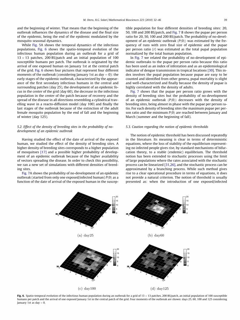
While Fig. 5A shows the temporal dynamics of the infectiouspopulations, Fig. 6 shows the spatio-temporal evolution of theinfectious human population during an outbreak for a grid of13 � 13 patches, 200 BS/patch and an initial population of 100susceptible humans per patch. The outbreak is originated by thearrival of one exposed human on January 1st at the central patchof the grid. Fig. 6 shows four pictures that represent four differentmoments of the outbreak (considering January 1st as day ¼ 0): theearly stages of the epidemic outbreak, characterized by the appear-ance of the first secondary infectious humans in the central andsurrounding patches (day 25), the development of an epidemic fo-cus in the center of the grid (day 60), the decrease in the infectiouspopulation in the center of the patch because of recovery and thespread of the disease in all directions resembling a cylindrical trav-elling wave in a reacto-diffusion model (day 100) and finally thelast stages of the outbreak because of the extinction of the adultfemale mosquito population by the end of fall and the beginningof winter (day 125).

5.2. Effect of the density of breeding sites in the probability of no-development of an epidemic outbreak

Having studied the effect of the date of arrival of the exposedhuman, we studied the effect of the density of breeding sites. Ahigher density of breeding sites corresponds to a higher populationof mosquitoes [17] and a possible higher probability of develop-ment of an epidemic outbreak because of the higher availabilityof vectors spreading the disease. In order to check this possibility,we ran a new set of simulations with different densities of breed-ing sites.

Fig. 7A shows the probability of no-development of an epidemicoutbreak (started from only one exposed/infected human) Pð0Þ as afunction of the date of arrival of the exposed human in the suscep-

0

5

10

15

20

0 2

4 6

8 10

12 0

2

4

6

8

10

12

0 5101520

0

5

10

15

20

0 2

4 6

8 10

12 0

2

4

6

8

10

12

0 5 10 15 20

Fig. 6. Spatio-temporal evolution of the infectious human population during an outbreakhumans per patch and the arrival of one exposed January 1st in the central patch of the gJanuary 1st as day ¼ 0.

tible population for four different densities of breeding sites: 20,50, 100 and 200 BS/patch, and Fig. 7 B shows the pupae per personratio for 20, 50, 100 and 200 BS/patch. The probability of no-devel-opment of an epidemic outbreak ðPð0ÞÞ was estimated by the fre-quency of runs with zero final size of epidemic and the pupaeper person ratio (r) was estimated as the total pupal populationnormalized by the total human population.

In Fig. 7 we related the probability of no-development of epi-demic outbreaks to the pupae per person ratio because this ratiohas been used as an index of infestation and as an epidemiologicalindicator of dengue transmission in tropical locations [30]. This in-dex involves the pupal population because pupae are easy to becounted and identified from other genera, pupal mortality is slightand well-characterized and finally because the density of pupae ishighly correlated with the density of adults.

Fig. 7 shows that the pupae per person ratio grows with thedensity of breeding sites but the probability of no-developmentof an epidemic outbreak ðPð0ÞÞ decreases with the density ofbreeding sites, being almost in phase with the pupae per person ra-tio. For each density of breeding sites the maximum pupae per per-son ratio and the minimum Pð0Þ are reached between January andMarch (summer and the beginning of fall).

5.3. Caution regarding the notion of epidemic thresholds

The notion of epidemic threshold has been discussed repeatedlyin the literature. Its meaning is clear in terms of deterministicequations, where the loss of stability of the equilibrium represent-ing no infected people gives rise, by standard mechanisms of bifur-cation theory, to a stable (endemic) equilibrium. The thresholdnotion has been extended to stochastic processes using the limitof large populations where the rates associated with the stochasticprocess can be linearized [31,26], and the stochastic process can beapproximated by a branching process. While such method givesrise to a clear operational procedure in terms of equations, it doesnot provide a natural criterion. The notion of threshold is usuallypresented as: when the introduction of one exposed/infected

0

5

10

15

20

0 2

4 6

8 10

12 0

2

4

6

8

10

12

0 5 10 15 20

0

5

10

15

20

0 2

4 6

8 10

12 0

2

4

6

8

10

12

0 5 10 15 20

for a grid of 13 � 13 patches, 200 BS/patch, an initial population of 100 susceptiblerid. Four moments of the outbreak are shown: days 25, 60, 100 and 125 considering

0 30 60 90 120 150 180 210 240 270 300 330 3600

0.2

0.4

0.6

0.8

1

out

brea

k. P

(0)

200 BS/patch100 BS/patch50 BS/patch20 BS/patch

0 30 60 90 120 150 180 210 240 270 300 330 360Time / days

0.01.02.03.04.05.06.07.08.0

Pupa

e pe

r pe

rson

rat

io. r

Prob

abili

ty o

f no

epi

dem

ic

A

B

Fig. 7. Probability of no-development of an epidemic outbreak ðPð0ÞÞ and pupae per person ratio (r) vs. the date of arrival of the exposed human in the susceptible populationfor different densities of breeding sites, 20, 50, 100 and 200 BS/patch.

40 M. Otero, H.G. Solari / Mathematical Biosciences 223 (2010) 32–46

individual into a community of susceptible individuals will notgive rise to a large outbreak with probability one, the system is be-low threshold. The criterion is associated with the necessary use ofthe word ‘‘large”. In natural sciences there is no ‘‘large” or ‘‘small”but rather ‘‘larger than” and ‘‘smaller than”.

Nevertheless, not always the introduction of an infective humanresults in a major epidemic. Two epidemiological scenarios arepossible, as it has been already shown in Fig. 3. Either no infectionor only a few individuals will become infected or else a large pro-portion of the population of susceptible humans will have been in-fected by the end of the epidemic [26], but no clear non-arbitrarythreshold can be computed from observations or simulations.

Several works have been carried out [7,8,10,13,12] in order tofind a suitable expression for the basic reproductive number R0

for dengue transmission. By R0 we understand the average numberof secondary cases arising from a single primary case in a largepopulation of susceptible humans, and it is used as an ordinarythreshold condition for the existence of an endemic state.

In 2000, Focks et al. attempted to develop dengue transmissionthresholds for several dengue-endemic or dengue-receptive tropi-cal locations in terms of the pupae per person ratio [30], and esti-mated this ratio in several conditions of constant temperatures andinitial seroprevalences of antibodies in the population. In particularthe ratio is approximately between 1 and 3 for constant tempera-tures between 24 and 26 degrees (according to daily mean temper-atures of the city of Buenos Aires in summer) and with an initialseroprevalence of antibody of 0%.

Considering Figs. 4 and 7 jointly, we see that the epidemic out-breaks for 200 BS that start on November 1st (day 123 in Fig. 7)present about 1 pupa per human and a probability of not develop-ing an epidemic of 0.8, but a possibility of having large epidemicoutbreaks. This is not precisely a disagreement between our workand that by Focks et al., but rather a necessary consequence of sea-sonal effects not included in the models by Focks. Such effects notalways take the form of summer-winter temperature differences,but even in tropical regions they are present as humid (rainy)-dry seasons.

According to our model, pupae per person ratios between 1 and3 would correspond to densities between 50 and 100 BS/patch andprobabilities of no-development of an epidemic outbreak Pð0Þbetween 0.75 and 0.45, respectively. Differences between bothmodels were not unexpected because even though the pupae per

person ratio might be a good estimate of A. aegypti infestation,its use as a dengue risk index is doubtful in temperate climateswhere the mosquito spatio-temporal dynamics modulates theepidemic outbreaks. We have already shown that very unlikelyepidemic outbreaks beginning at the end of spring could lead tolarge final sizes of epidemics.

In 1964, M. S. Bartlett proposed a simple analytical expressionfor the probability of no major epidemics started from only one in-fected human [31]. This probability Q � is given by Eqs. (11) and(12). We must keep in mind that in Bartlett’s model, vector popu-lations and infection rates were considered constant (no seasonaleffects) although he was inspired in malaria (a comprehensiveretelling of Bartlett results can be found in [32]).

Q � ¼ l1 � ðl2 þ k1 � ShÞk1 � Shðl1 þ k2 � SvÞ ð11Þ

or

Q � ¼ 1 ð12Þ

whichever is the smaller and where Sh is the initial population ofsusceptible humans, Sv is the initial population of susceptible vec-tors, k1 is the rate of infection for humans per susceptible humanper infected vector, k2 is the rate of infection for vectors per suscep-tible vector and infected human and l1 and l2 are the removal ratesfor infected humans and vectors, respectively.

According to our model, the parameters of Bartlett’s model can beexpressed as: k1 ¼ cycle2 � avh; k2 ¼ cycle1 � ahv;l1 ¼ ð1=VPÞ;l2 ¼ma; Sh ¼ Nhði;jÞ and Sv ¼ Av ði;jÞ which is the total adult female vectorpopulation whose dynamics are seasonal. Then a Bartlett-like esti-mate of Pð0Þ is given by Eqs. (13) and (14).

Q � ¼ ð1=VPÞ � ðmaþ cycle2 � avh � Nhði;jÞÞcycle2 � avh � Nhði;jÞðð1=VPÞ þ cycle1 � ahv � Av ði;jÞÞ

ð13Þ

or

Q � ¼ 1 ð14Þ

whichever is the smaller and where cycle1 and cycle2 are thegonotrophic cycle rate coefficients (see Appendix B), ahv is thetransmission probability from host to vector, avh is the transmis-sion probability from vector to host, ðahv ¼ avh ¼ 0:75Þ;VP is theviremic period ðVP ¼ 3 daysÞ;ma is the mortality coefficient of

M. Otero, H.G. Solari / Mathematical Biosciences 223 (2010) 32–46 41

adult vectors ma ¼ 0:091 days�1 and Nhði;jÞ and Av ði;jÞ are thehuman and adult female vector populations per patch respec-tively.

Fig. 8 shows the Pð0Þ values obtained with our model (with 0.90confidence intervals) vs the date of arrival of the exposed human inthe susceptible population for different densities of breeding sites(20, 50, 100 and 200 BS/patch) and, for comparison, results derivedfrom a Bartlett-like Model, Eq. (13). First, notice that the Bartlettmodel assumes a constant vector population, which we took asthe population of the day the first infectious individual is placed.Second, Bartlett’s model produces the probability of not having amajor outbreak ðP�Þ where as already explained, major has no pre-cise meaning, but we know that P� P Pð0Þ. Finally, Q � is an approx-imation to P� that not only simplifies the biological problem butalso introduces linear rates instead of the non-linear rates of theproblem. The way in which the linearization is performed disre-gards the slowing down (and eventually ceasing) of the epidemicoutbreak by the exhaustion of susceptible individuals and satura-tion of exposed vectors. Since P� P Q � and P� P Pð0Þ the relationbetween Q � and Pð0Þ is not fixed a priori.

Fig. 8 shows that for low vector densities (20 and 50 BS/patch) Q � > Pð0Þ. We see that Q � would suggest zero probabilityof large epidemic outbreaks starting on November 1st or May1st even for 200 BS/patch, although both situations are quite dif-ferent. Epidemics starting on May 1st have no chance to developinto large epidemic outbreaks but those starting on November1st can produce major outbreaks although with small frequency.When the epidemic outbreaks start near the maximum of themosquito population (February 1st) the estimation by Eq. (13)goes from excess at 20 BS/patch to defect at 200 BS/patch corre-sponding to the increase in the abundance of vectors and thecorresponding improved performance of the linearization. For20 BS/patch, the predicted epidemic outbreaks starting on Janu-ary 1st involve 14 cases. However, whether 14 cases representa not-large epidemic outbreak in a region with no precedentsof dengue is a matter of public policy and cannot be settled bymathematical criteria completely unrelated to public healthcriteria.

0 30 60 90 120 150 180

0.20.40.60.8

1

P(0)

0 30 60 90 120 150 180

0.20.40.60.8

1

P(0)

0 30 60 90 120 150 180.20.40.60.8

1

P(0)

0 30 60 90 120 150 18Time

0.4

0.6

0.81

P(0)

200 BS

100 BS

50 BS

20 BS

Fig. 8. Probability of no-development of an epidemic outbreak (with 0.90 confidence intdifferent densities of breeding sites, 20, 50, 100 and 200 BS/patch and comparison with

6. Miscellaneous discussion

6.1. Dengue and yellow fever

Dengue and yellow fever are two kinds of encephalitis that pro-duce hemorrhagic fever. At the level of description explored in thepresent work they are not distinguishable, except perhaps for dif-ferent characteristic times of the clinical phase and the extrinsiccycle of the virus.

From a clinical point of view, the main difference betweendengue and yellow fever is the mortality of the toxic period. Inboth diseases, fever takes a saddle back pattern, with fever drop-ping or disappearing during some hours (up to 48 h) followed bya re-emergence [34,37]. In yellow fever, this second febrile periodis called the ‘‘toxic period” and occurs in about 15–25% of the cases[33], leading to death in about half of them. The toxic period in yel-low fever is not contagious and as such does not change thedynamics of the epidemic.

From a virological point of view, dengue and yellow fever areproduced by two flaviviruses of the Flaviviridae family [35].

The involved vector in the Americas for urban yellow fever anddengue is the same mosquito: A. aegypti [20,36,35].

The immunological response to these viruses is so similar thatthe IgG-ELISA and hemagglutination-inhibition tests cannot distin-guish between flaviviruses [37]. It has been argued that denguecould provide immunity for yellow fever, an argument that hasbeen later proven wrong by experiments in mice [38]. Yet, chime-ric dengue vaccines are being sought as modified yellow fever vac-cines [39], a project that exploits similarities at the molecular levelof both viruses.

All the similarities described indicate that our dengue modelcan be used, with a proper choice of parameters, to simulate urbanyellow fever outbreaks, as discussed in [35] for simpler models.

6.2. Choice of parameters for dengue

The quantitative details of dengue transmission are not com-pletely known, in part because clinical manifestations of dengue

0 210 240 270 300 330 360

Bartlett ModelModel ResultsConfidence Intervals

0 210 240 270 300 330 360

0 210 240 270 300 330 360

0 210 240 270 300 330 360 / days

ervals) vs the date of arrival of the exposed human in the susceptible population forresults predicted by Bartlett Model.

Table 8Comparison of dengue transmission parameters in different works. The present workfollows [7]. The values extracted from [41] are direct elaboration of experimentaldata. IIP = intrinsic incubation period; ATT = average time virus transmission (humanto mosquito); IIP + ATT = characteristic time from onset of dengue and mosquitoinfection; W = accumulated weight factor of virus transmission and WV = window ofviremia.

Work IIP/days ATT/days I + ATT/days W WV/days

Newton [7] 5 3 8 2.25 —Focks [15] 4 0–5 4–9 1.5–2.75 5Chowell [40] 5.5 �2.5 �8 �0.98 —Nishiura [41] 4 (DEN1) 2.38 6.38 3.5 5

42 M. Otero, H.G. Solari / Mathematical Biosciences 223 (2010) 32–46

do not follow immediately the inoculation of the virus by themosquito. The acute febrile period begins after 3–14 days ofinoculation [2] (Gubler reports that averages are in the range of4–7 days [37]). During the febrile period, which lasts between 2and 19 days, dengue viruses can circulate in the peripheral blood[[37]p484]. Since these numbers are conditioned to those peoplereporting dengue symptoms, thus asymptomatic and subclinicalcases are not part of the sample adding more uncertainties to thedescription. In addition, ‘‘viremia usually peaks at the time orshortly after the onset of illness and may remain detectable for var-ious periods ranging from 2 to 12 days” [[37], p. 487].

More uncertainties are added by the various kinds of modelsused for dengue. In a first group we have the stochastic modelswith exponentially distributed times and their deterministic limitssuch as in [7,9,10] and this work. These works follow Newton andReiter [7] in their choice of parameters, with an average intrinsicincubation period of 5 days and average viremic period of 3 days.

A second set of parameters is used by Focks et al. [15]. The de-fault value for the duration of the incubation period is of 4 daysand for the duration of viremic period is of 5 days. The preciseway in which this parameter is used is not clear, presumably inan accounting program (also called dynamics time table). Afterbeing infected, people enter the incubation stage and after 4 daysmove into the viremic phase, which lasts 5 days. To add furthercomplexity, the transmission of virus to the biting mosquito re-sponds to the level of viremic titer, whose form changes alongthe viremic period.

A third and last set of parameters is used in a deterministicmodel implementing the so-called linear-chain-trick [40]. In thiscase the mean intrinsic incubation period is of 5.5 days and theviremic period has a mean of 5 days (These averages correspondto incomplete gamma distributions associated with 54 and 25exponentially distributed steps).

It is clear that the three families of models rely heavily on whatis possible to simulate. Existing data are scarce. Experiments per-formed with human beings before World War II are perhaps thebest source of data. Recently two of these experiments have beenrevisited [41].

The incubation period is defined in [41] as the time from themosquito bite until the day of the onset of the illness (i.e., fever),and averages 6 days (DEN4) and 5.7 days (DEN1) with cases asearly as 3 days and as late as 10 days. The viremic period is countedfrom the onset of classical dengue symptoms (day zero) and ex-tends from �2 to 3 days (i.e., the possibility of infecting a mosquitocan precede 2 days the appearance of clinical symptoms). In orderto compute Virus Transmission Rates ðVTRðtÞÞ, counting by daysfrom the inoculation, we need to perform the convolution

Z t

0/Incðt � sÞgðsÞds ð15Þ

where /IncðsÞ is the probability density distribution for the incuba-tion time and gðsÞ the probability of infecting a mosquito at the times after the onset of the contagious period (i.e., gðtÞ is zero fort R ½0;WV � where WV is the limit of the window for viremia). Theexperimental function reported in [41] has WV ¼ 5 days, the accu-mulated weight factor of virus transmission is W ¼

RWV0 gðsÞds ¼

3:5, the average time of incubation (i.e., before viremia) is 4 days(DEN4) and 3.7 days (DEN1) and the average transmission time isATT ¼

RWV0 sgðsÞds=W , which takes the value ATT ¼ 2:38 days count-

ing from the start of the viremic period.The interpretation of the identified characteristics is as follows:

assume that susceptible mosquitoes bite at a constant rate b andthat the time is counted from the beginning of the viremic period.When t > WV there are no viruses transmitted to the mosquitoes.The average number of infected mosquitoes per viremic person is

then W b , while the average time when a mosquito loaded thevirus is ATT. When the viremic period is exponentially distributedwith parameter VP and the transmission probability from host tovector is ahv, we have W ¼ VP ahv and ATT ¼ VP.

It is extremely important to notice that the incubation period asdefined by Gubler [37] and by Nishiura and Halstead [41] differs inmeaning with the incubation period given in modelling worksincluding those by Focks et al. [15], Chowell et al. [40] and thiswork. Incubation period refers to the time from virus inoculationto fever in [37,41] and from virus inoculation to the beginning ofthe infective period here and in [15,40].

We summarize the results corresponding to the data and mod-els in Table 8. Notice that the value of W will only be relevant whennot only the evolution of the epidemic but also the adult mosquitopopulation is measured, since the mosquito population (or thenumber of breeding sites in this work) is roughly a multiplicativefactor in front of gðsÞ.

When the human viremic period is changed in the model, bothATT and W change according to the assumed exponential distribu-tion of the viremic time. As W increases, we expect a larger pro-portion of mosquitoes infected and thus more circulation of thevirus and larger final size of the epidemic. However, the oppositeeffect may occur to a lesser degree since it takes a longer averagetime for a mosquito to load the virus, reducing the number ofcontagious cycles prior to winter, and resulting in smaller out-breaks. We illustrate these effects in Fig. 9. All the plots corre-spond to the final size of an epidemic started with the arrivalof one infected person on January 1st and correspond to an envi-ronment with A. aegypti sustained in the equivalent to 200 breed-ing sites. The plot in the center is the same plot shown in Fig. 4for January, repeated to facilitate the comparison. On top, onlythe viremic period has been changed from 3 to 5 days, resultingin larger epidemics as expected. The bottom plot presents thesame change in viremic period with the additional change ofahv (7) from 0.75 to 0.45 to compensate the change of W. Wecan see then how the effect of a longer period produces smallerepidemics when the infected mosquitoes are compensated byother parameters.

6.3. A first encounter with (real) dengue

The history of dengue in Argentina has been resumed in Appen-dix A, but the account in the appendix was up to the date of sub-mission of the initial version of this work.

Between the date of the first version and that of the revised ver-sion, the largest ever epidemic of dengue in Argentina developed.With several simultaneously active focus disseminated throughthe country, such as in Charata, Catarmarca, Tartagal, Oran, Tuc-umán and other cities, dengue virus began to circulate throughthe country. In retrospect, the initial cases emerged at the begin-ning of January while the peak of the epidemic was around mid-April [42].

0 2000 4000 6000 8000 10000Final size of Epidemic

0

5

10

15

20

Freq

uenc

y in

100

run

s0 2000 4000 6000 8000 10000

0

5

10

15

20

0 2000 4000 6000 8000 100000

5

10

15

20

Fig. 9. Frequency of the total number of infected people in 100 simulations of epidemic outbreaks starting on January 1st for 200 breeding sites per block. Top, viremic periodof 5 days (ATT = 5 days, W = 3.75). Middle, viremic period of 3 days (ATT = 3 days, W = 2.25) and bottom, viremic period of 5 days (ATT = 5 days, W = 2.25).

M. Otero, H.G. Solari / Mathematical Biosciences 223 (2010) 32–46 43

During the year, a total of 106 imported cases were confirmed inthe city of Buenos Aires. However, potential local cases were rou-tinely dismissed until the end of March enforcing the belief that den-gue transmission was not possible in the region. The total of localcases confirmed so far is of 20. During the same period of time only72 imported cases were confirmed (the geographical distribution ofcases presents higher density in the quarter of Mataderos than inother regions of the city). Assuming an equal handling of local andimported cases, the ratio between local cases and total cases (R) isR � 20

92 � 0:22, while our computations for Mataderos (a districtwhich has the largest recorded infestation of A. aegypti) are in therange: 0:05 6 R 6 0:76 for infected people arriving on April 1st(see Fig. 10). The range computed corresponds to the intrinsic diffi-culties of estimating the number of breeding sites in the area.

While a detailed calculation is for the time being not possiblesince details of the information are not available, we notice thatthe model scales in the limit of large numbers with the numberof breeding sites, provided the ratio BS/human is kept constant.In this extreme simplification, the data of the city of Buenos Aires

0 0.5Breeding s

0

0.2

0.4

0.6

0.8

Loc

al D

engu

e ca

ses

/ (To

tal c

ases

)

Fig. 10. Ratio between local cases and total cases in 100 runs (R) compute

correspond to 0:5 BS=human according to our calculations. How-ever, data available for the great Buenos Aires area (which includesseveral satellite cities making a continuous urbanization) producean estimate of R ¼ 0:58 which roughly corresponds to small epi-demic scenarios computed for ratios of about 1:5 BS/human. Thesedata must be considered with extreme caution because reports ofconfirmed cases are still changing.

The model has then survived its first encounter with denguetransmission, being able to predict without any tuning, that theecological conditions in the city of Buenos Aires (and its extendedarea) made it possible the circulation of the dengue to a limited ex-tend, for infected people arriving by late March and early April.According to the model, the date of arrival has been crucial for thisoutcome and more dangerous epidemic situations would developin case of arrivals earlier in the year.

The data made so far available by the Health authority do notmake it possible a deeper analysis. We can only hope that theinformation will be made available in the future so that more de-tailed checks can be performed on the model.

1 1.5 2ites/Human

d for different ratios of breeding sites to human beings in Mataderos.

44 M. Otero, H.G. Solari / Mathematical Biosciences 223 (2010) 32–46

7. Summary and conclusions

We have developed a stochastic dynamical model for the trans-mission of dengue that takes into account the seasonal and spatialdynamics of the vectors and describes the disease dynamics trig-gered by the arrival of infected people in the city and modulatedby the seasonal and the spatial vector dynamics.

The model takes into account the populations of both hosts(Humans) and vectors (A. aegypti), which are divided into subpop-ulations representing the disease status: susceptible (S), exposed(E) and infectious (I) for adult female vectors and susceptible (S),exposed (E), infectious (I) and removed (R) for humans. The trans-mission of only one serotype of virus is considered and mechanicaltransmission (i.e., without amplification of the virus in the vector)is not taken into account. The evolution of the populations is con-sidered in terms of random events with transition probabilitiesprescribed in terms of the mosquito biology, the disease evolutionand the local environment. The model can be easily extended toother diseases propagated by Aedes aegypti such as yellow fever.

While any model is reductionist, we have tried to build ourmodel avoiding as much as possible simplifying hypotheses (i.e.,hypotheses with dubious biological support introduced only torender the calculations simpler). We actually intended to producea simple but realistic model, where the different biological pro-cesses are reflected and acknowledged. Our expectation is that incase the model is shown not to agree with field research, the falsa-tion will move up to the hypotheses and a piece of ignored or mis-understood biology will be unearthed. Despite the very largenumber of parameters required by the model, there are no freeparameters to fit the model to the observations, not even the num-ber of active breeding sites ðBSÞ which are hard to evaluate but nothard to estimate.

We showed that the date of arrival of an exposed/infected hu-man in a susceptible human population dramatically affects thedistribution of the final size of the epidemics. Outbreaks startingwith the arrival of the exposed in the late spring, have a lesserprobability to evolve, but those that eventually develop are likelyto produce large epidemic outbreaks because they have a longertime to evolve until the extinction of the adult female vector pop-ulation at the beginning of winter. In the contrary, a later arrival ofthe exposed in summer (even if the probability of an epidemic out-break is higher) produces outbreaks with lower populations ofinfectious humans because the end of the epidemics is modulatedby the progressive extinction of the adult female mosquitoes bythe end of the autumn season.

Furthermore, when conditions are favorable for the spreading ofdengue in summer, the epidemic outbreak is quenched by theextinction of the adult female population in winter. When the loca-tion presents a seasonal dependence of climatic conditions, andone season is sufficiently adverse to the mosquito to prevent thespread of dengue, the probability of secondary cases will stronglydepend on the basic reproductive number and on the time ofarrival of the exposed person. Yet, even in situations below the epi-demic threshold [31] not significantly large epidemics can sustainthe circulation of the virus until favorable conditions for a largeepidemic are reached. Seasonal climatic variations not only includetemperature as considered here, but also humid-dry periods as inthe cases studied in [16].

We believe that the results presented make a strong case for thenecessity of predictive models as opposed to ‘‘criteria”. If preven-tive measures are to be taken in time to be useful, and not lateas quite often happens, it is necessary to predict the evolution ofmosquito populations and the viral disease according to the realsituation. Actually, mathematical models have the advantage ofmaking explicit the predictive mechanism while criteria, onceseparated from the originating work, appear as universal conclu-

sions, as they leave for the user the verification of hiddenhypotheses.

Our model could be used as a mathematical tool to study differ-ent epidemic scenarios in urban environments and to estimate therisk and final size of epidemic outbreaks in temperate cities whereseasonal temperature changes cannot be ruled out. For general use,the model needs to incorporate the dry-humid cycle. Work is inprogress in this direction as well, but we anticipate that currentbiological knowledge on this matter is not as accurate as theknowledge of the temperature influence, and the development ofan improved model runs in parallel with the development of bio-logical understanding.

Having formulated a model that intends to be almost as realisticas possible under present knowledge of the problem, we intend to‘‘validate” it by contrasting its results with real epidemic observa-tions. The recent circulation of the virus in the target region will of-fer a good opportunity for validation. The model can be easilyadapted to other regions using the appropriated climatic data,and further validation and/or tuning can be achieved in this form.Furthermore, since the model can also be easily adapted to yellowfever outbreaks (as discussed in Section 6.1), the eco-epidemiolog-ical approach supported in the description of the mosquito A. ae-gypti can be tested with the historical records of urban yellowfever epidemics. The reconstruction of the historic epidemic of1871, with its more than 13,000 death cases will be the subjectof a separate study.

The discussion regarding the choice of parameters in Section 6indicates that compensatory effects may occur. Epidemic datamay not be enough to determine, indirectly, parameter choices un-less the details of the epidemic outbreak are considered and themosquito abundance is sampled. The data recently made availableby Nishiura and Halstead [41] suggest that all the existing denguemodels will fail at one point or another, and that new forms ofmodelling are needed to achieve further realism.

Acknowledgements

The authors acknowledge CONICET and the support given bythe University of Buenos Aires under Grant X308 (2004–2007),X210 (2008–2010) and by the Agencia Nacional de PromociónCientf́ica y Tecnológica (Argentina) under Grants PICTR 87/2002and PICT 00932/2006.

Appendix A. A brief history of dengue fever in Argentina

In 1916 an epidemic of dengue in Argentina, introduced fromParaguay, affected the cities of Concordia (Corrientes) and Paraná(Entre Rios). In 1947 the Pan-american Health organization(PHO) led a continental mosquito eradication program which con-sisted of the use of insecticides and the systematic destruction ofwater containers [43]. By 1967 the mosquito was considered tobe eradicated in 18 countries including Argentina. In 1986 themosquito was detected in Posadas, Puerto Iguazú and other citiesin northern Argentina, and finally in the city of Buenos Aires by1995. In 1997 DEN2 cases were detected in cities of Salta such asOrán, Salvador Mazza, Güemes and Tartagal and in 1998 an epi-demic outbreak of DEN2 in the region of the Chaco Salteño withepicenter in the city of Tartagal caused 359 confirmed cases [44].From December 1999 to May 2000 the Muñiz Infectology Hospitalof Buenos Aires received 50 patients infected with dengue (DEN1)imported mainly from an extended epidemic in Paraguay [6]. In2000 two DEN1 epidemic outbreaks were reported in Misionesand Formosa, both outbreaks probably originated from importedcases from neighboring endemic countries. In 2002 DEN3 appearedin Misiones and 214 DEN1 cases were detected in Salta. A total of

M. Otero, H.G. Solari / Mathematical Biosciences 223 (2010) 32–46 45

98 confirmed cases were reported in the country in 2003 [44], andin 2004 an extended outbreak of DEN3 took place in the cities ofSalvador Mazza, Orán, Tartagal, Embarcación, Aguaray and Picha-nal [6]. The situation in the northwestern region became worsein 2006 because of floodings mainly in the city of Tartagal. Smalloutbreaks took place not only in the northwestern region (ChacoSalteño) but also in the northeastern region (Iguazú), with 55and 90 reported cases respectively.

Appendix B. Temperature model and parameter values

B.1. Temperature model

A very simple model for the mean daily temperature variation,which contains only the deterministic component of the tempera-tures, was used in this work. The model was chosen from [45] andtakes the form:

T ¼ aþ b cos2pt

365:25daysþ c

� �ð16Þ

with time measured in days beginning on the first of July. Theparameters a, b and c were fitted from temperature records alonga period of time of 10 years and are: a ¼ 18:0 �C;b ¼ 6:7 �C andc ¼ 9:2. The use and development of this model is detailed in[17].

B.2. Developmental rate coefficients

The developmental rates that correspond to egg hatching, pupa-tion, adult emergence and the gonotrophic cycles were evaluatedusing the results of the thermodynamic model developed by Sharpand DeMichele [46] and simplified by Schoofield et al. [47]. Accord-ing to this model, the maturation process is controlled by only oneenzyme which is active in a given temperature range and is deac-tivated only at high temperatures. The development is stochastic innature and is controlled by a Poisson process with rate RDðTÞ. Ingeneral terms RDðTÞ takes the form

RDðTÞ ¼ RDð298 �KÞ

� ðT=298 �KÞ � expððDHA=RÞð1=298 �K� 1=TÞÞ1þ expðDHH=RÞð1=T1=2 � 1=TÞ ð17Þ

where T is the absolute temperature, DHA and DHH are thermody-namics enthalpies characteristic of the organism, R is the universalgas constant, and T1=2 is the temperature when half of the enzyme isdeactivated because of high temperature.

Table 9 presents the values of the different coefficients involvedin the events: egg hatching, pupation, adult emergence and gono-trophic cycles. The values are taken from [48] and are discussed in[17].

Table 9Coefficients for the enzymatic model of maturation (Eq. (17)). RD is measured inday�1, enthalpies are measured in (cal/ mol) and the temperature T is measured inabsolute (Kelvin) degrees.

Develop. cycle (17) RDðTÞ RDð298�KÞ DHA DHH T1=2

Egg hatching elr 0.24 10,798 100,000 14,184Larval develop. lpr 0.2088 26,018 55,990 304.6Pupal develop. par 0.384 14,931 �472,379 148Gonotrophic c. ðA1Þ Cycle1 0.216 15,725 1,756,481 447.2Gonotrophic c. ðA2Þ Cycle2 0.372 15,725 1,756,481 447.2

B.3. Mortality coefficients

B.3.1. Egg mortalityThe mortality coefficient of eggs is me ¼ 0:011=day, indepen-

dent of temperature in the range 278 �K 6 T 6 303 �K [49].

B.3.2. Larval mortalityThe value of a0 (associated with the carrying capacity of a single

breeding site) is a0 ¼ 1:5 and was assigned by fitting the model toobserved values of immatures in the cemeteries of Buenos Aires[17]. The temperature-dependent larval death coefficient isapproximated by ml ¼ 0:01þ 0:9725 expð�ðT � 278Þ=2:7035Þ andis valid in the range 278 �K 6 T 6 303 �K [50–52].

B.3.3. Pupal mortalityThe intrinsic mortality of a pupa has been considered as

mp ¼ 0:01þ 0:9725expð�ðT � 278Þ=2:7035Þ [50–52]. Besides thedaily mortality in the pupal stage, there is an additional mortalityassociated with the emergence of the adults. We consider a mortal-ity of 17% of the pupae at this event, which is added to the mortal-ity rate of pupae, hence the emergence factor is ef ¼ 0:83 [19].

B.3.4. Adult mortalityAdult mortality coefficient is ma ¼ 0:091=day and is considered

independent of temperature in the range 278 �K 6 T 6 303 �K[50,20,53].

B.4. Fecundity and oviposition coefficient

Females lay a number of eggs that is roughly proportional totheir body weight ð46:5 eggs=mgÞ [54,55]. Considering that themean weight of a three-day-old female is 1:35 mg [20], we esti-mate the average number of eggs laid in one oviposition asegn ¼ 63.

The oviposition coefficient ovrði;jÞ depends on breeding site den-sity BSði;jÞ and is defined as:

ovrði;jÞ ¼h=tdep if BSði;jÞ 6 1501=tdep if BSði;jÞ > 150

(ð18Þ

where h was chosen as h ¼ BSði;jÞ=150, a linear function of the den-sity of breeding sites [18].

B.5. Dispersal coefficient

We chose a diffusion-like coefficient of diff = 830 m2/day whichcorresponds to a short dispersal, approximately a mean dispersalof 30 m in one day, in agreement with short dispersal experimentsand field studies analyzed in detail in our previous article [18].

References

[1] M. Hunt, Microbiology and Immunology On-line, University of South Carolina,School of Medicine, South Carolina, United States, 2007, Available from<http://www.med.sc.edu:85/mhunt/arbo.htm>.

[2] WHO, Dengue hemorrhagic fever, in: Diagnosis Treatment Prevention andControl, second ed., World Health Organization, Ginebra, Suiza, 1998.

[3] N. Schweigmann, R. Boffi, Aedes aegypti y aedes albopictus: Situaciónentomológica en la región, in: Temas de Zoonosis y EnfermedadesEmergentes, Segundo Cong. Argent. de Zoonosis y Primer Cong. Argent. yLationoamer. de Enf. Emerg. y Asociación Argentina de Zoonosis, Buenos Aires,1998, p. 259.

[4] A.B. de Garı́n, R.A. Bejarán, A.E. Carbajo, S.C. de Casas, N.J. Schweigmann,Atmospheric control of Aedes aegypti populations in buenos aires (argentina)and its variability, International Journal of Biometerology 44 (2000) 148.

[5] A.E. Carbajo, N. Schweigmann, S.I. Curto, A. de Garı́n, R. Bejarán, Denguetransmission risk maps of argentina, Tropical Medicine and InternationalHealth 6 (3) (2001) 170.

[6] A. Seijo, Situación del dengue en la argentina, Boletín de la AsociaciónArgentina de Microbiología 175 (2007) 1.

46 M. Otero, H.G. Solari / Mathematical Biosciences 223 (2010) 32–46

[7] E.A.C. Newton, P. Reiter, A model of the transmission of dengue fever with anevaluation of the impact of ultra-low volume (ulv) insecticide applications ondengue epidemics, American Journal of Tropical Medicinal Hygiene 47 (1992)709.

[8] L. Esteva, C. Vargas, Analysis of a dengue disease transmission model,Mathematical Biosciences 150 (1998) 131.

[9] L. Esteva, C. Vargas, A model for dengue disease with variable humanpopulation, Journal of Mathematical Biology 38 (1999) 220.

[10] L. Esteva, C. Vargas, Influence of vertical and mechanical transmission on thedynamics of dengue disease, Mathematical Biosciences 167 (2000) 51.

[11] L.M. Bartley, C.A. Donnelly, G.P. Garnett, The seasonal pattern of dengue inendemic areas: mathematical models of mechanisms, Transactions of theRoyal Society of Tropical Medicine and Hygiene 96 (2002) 387.

[12] P. Pongsumpun, I.M. Tang, Transmission of dengue hemorrhagic fever in anage structured population, Mathematical and Computer Modelling 37 (2003)949.

[13] M. Derouich, A. Boutayeb, E.H. Twizell, A model of dengue fever, BiomedicalEngineering Online 2 (2003) 4.

[14] A. Tran, M. Raffy, On the dynamics of dengue epidemics from large-scaleinformation, Theoretical Population Biology 69 (2006) 3.

[15] D.A. Focks, D.C. Haile, E. Daniels, D. Keesling, A simulation model of theepidemiology of urban dengue fever: literature analysis, model development,preliminary validation and samples of simulation results, American Journal ofTropical Medicinal Hygiene 53 (1995) 489.

[16] L.B.L. Santos, M.C. Costa, S.T.R. Pinho, R.F.S. Andrade, F.R. Barreto, M.G. Teixeira,M.L. Barreto, Periodic forcing in a three level cellular automata model for avector transmitted disease, arXiv:0810.0384v1, 2008.

[17] M. Otero, H.G. Solari, N. Schweigmann, A stochastic population dynamic modelfor Aedes aegypti: formulation and application to a city with temperateclimate, Bulletin of the Mathematical Biology 68 (2006) 1945.

[18] M. Otero, N. Schweigmann, H.G. Solari, A stochastic spatial dynamical modelfor Aedes aegypti, Bulletin of Mathematical Biology 70 (2008) 1297.

[19] T.R.E. Southwood, G. Murdie, M. Yasuno, R.J. Tonn, P.M. Reader, Studies on thelife budget of Aedes aegypti in wat samphaya Bangkok Thailand, Bulletin of theWorld Health Organisation 46 (1972) 211.

[20] R. Christophers, Aedes aegypti (L.), the yellow fever mosquito, CambridgeUniversity Press, Cambridge, 1960.

[21] A.E. Carbajo, S.I. Curto, N. Schweigmann, Spatial distribution pattern ofoviposition in the mosquito Aedes aegypti in relation to urbanization inbuenos aires: southern fringe bionomics of an introduced vector, Medical andVeterinary Entomology 20 (2006) 209.

[22] M. Wolfinsohn, R. Galun, A method for determining the flight range of Aedesaegypti (linn.), Bullentin of the Research Council of Israel 2 (1953) 433.

[23] P. Reiter, M.A. Amador, R.A. Anderson, G.G. Clark, Short report: dispersal ofAedes aegypti in an urban area after blood feeding as demonstrated byrubidium-marked eggs, American Journal of Tropical Medicinal Hygiene 52(1995) 177.

[24] J.D. Edman, T.W. Scott, A. Costero, A.C. Morrison, L.C. Harrington, G.G. Clark,Aedes aegypti (diptera culicidae) movement influenced by availability ofoviposition sites, Journal of Medicinal Entomology 35 (4) (1998) 578.

[25] S.N. Ethier, T.G. Kurtz, Markov Processes, John Wiley and Sons, New York,1986.

[26] H. Andersson, T. Britton, Stochastic epidemic models and their statisticalanalysis, Lecture Notes in Statistics, vol. 151, Springer-Verlag, Berlin, 2000.

[27] H.G. Solari, M.A. Natiello, Stochastic population dynamics: the poissonapproximation, Physical Review E 67 (2003) 031918.

[28] J.P. Aparicio, H.G. Solari, Population dynamics: a Poissonian approximation andits relation to the langevin process, Physical Review Letters 86 (2001) 4183.

[29] A.E. Carbajo, S.M. Gomez, S.I. Curto, N. Schweigmann, Variación espaciotemporal del riesgo de transmisión de dengue en la ciudad de buenos aires,Medicina 64 (2004) 231.

[30] D.A. Focks, R.J. Brenner, J. Hayes, E. Daniels, Transmission thresholds fordengue in terms of Aedes aegypti pupae per person with discussion of theirutility in source reduction efforts, American Journal of Tropical MedicinalHygiene 62 (1) (2000) 11.

[31] M.S. Bartlett, The relevance of stochastic models for large-scaleepidemiological phenomena, Applied Statistics 13 (1) (1964) 2.

[32] A.L. Lloyd, J. Zhang, A.M. Root, Stochasticity and heterogeneity in host vectormodels, Interface 4 (2007) 851.

[33] WHO, Yellow Fever, World Health Organization, Ginebra, Suiza, 2001, factsheet 100.

[34] J.S. Simmons, Dengue fever, The American Journal of Tropical Medicine XI(1933) 77.

[35] E. Massad, F.A.B. Coutnho, M.N. Burattini, L.F.F. Lopez, The risk of yellow feverin a dengue-infested area, Transactions of the Royal Society of TropicalMedicine and Hygiene 95 (2001) 370.

[36] P.N. Dégallier, J.P. Hervé, A.F.A.T.D. Rosa, G.C. Sa, Aedes aegypti (l.): Importancede sa bioécologie dans la transmission de la dengue et des autres arbobirus,Bulletin des Societes Pathologie Exotique 81 (1988) 97.

[37] D.J. Gubler, Dengue and dengue hemorrhagic fever, Clinical MicrobiologyReview 11 (1998) 480.

[38] J. Vainio, F. Cutts, Yellow fever, Tech. Rep., World Health Organization, Geneva,1998.

[39] R.G. van der Most, K. Murali-JKrishna, R. Ahmed, J.H. Strauss, Chimeric yellowfever/dengue virus as a candidate dengue vaccine: quantitation of the denguevirus-specific cd8 t-cell response, Journal of Virology 74 (2000) 8094.

[40] G. Chowella, P. Diaz-Dueñas, J. Miller, A. Alcazar-Velazco, J. Hyman, P.Fenimore, C. Castillo-Chavez, Estimation of the reproduction number ofdengue fever from spatial epidemic, Mathematical Biosciences 208 (2007)571.

[41] H. Nishiura, S.B. Halstead, Natural history of dengue virus (denv)-1 and denv-4infections: Reanalysis pf classic studies, Journal of Infectious Diseases 195(2007) 1007.

[42] Actualización casos de dengue en argentina, 10 de mayo de 2009, Tech. rep.,Ministerio de Salud Pública de Argentina, Buenos Aires, 2009, Available from<http://www.msal.gov.ar/htm/Site/sala_situacion/index.asp>.

[43] Campaña de erradicacion del Aedes aegypti en la república argentina. informefinal, Tech. Rep., Ministerio de Asistencia Social y Salud Publica, Argentina,Buenos Aires, 1964.

[44] C. Rotela, F. Fouque, M. Lamfri, P. Sabatier, V. Introini, M. Zaidenberg, C.Scavuzzo, Space-time analysis of the dengue spreading dynamics in the 2004tartagal outbreak northern argentina, Acta Tropica 103 (2007) 1.

[45] A. Király, I.M. Jánosi, Stochastic modelling of daily temperature fluctuations,Physical Review E 65 (2002) 051102.

[46] P.J.H. Sharpe, D.W. DeMichele, Reaction kinetics of poikilotherm development,Journal of Theoretical Biology 64 (1977) 649.

[47] R.M. Schoofield, P.J.H. Sharpe, C.E. Magnuson, Non-linear regression ofbiological temperature-dependent rate models based on absolute reaction-rate theory, Journal of Theoretical Biology 88 (1981) 719.

[48] D.A. Focks, D.C. Haile, E. Daniels, G.A. Moun, Dynamics life table model forAedes aegypti: analysis of the literature and model development, Journal ofMedical Entomology 30 (1993) 1003.

[49] M. Trpis, Dry season survival of Aedes aegypti eggs in various breeding sites inthe dar salaam area, tanzania, Bulletin of the World Health Organisaion 47(1972) 433.

[50] W.R. Horsfall, Mosquitoes: Their Bionomics and Relation to Disease, Ronald,New York, USA, 1955.

[51] M. Bar-Zeev, The effect of temperature on the growth rate and survival of theimmature stages of Aedes aegypti, Bulletin of the Entomological Research 49(1958) 157.

[52] L.M. Rueda, K.J. Patel, R.C. Axtell, R.E. Stinner, Temperature-dependentdevelopment and survival rates of culex quinquefasciatus and Aedes aegypti(diptera: Culicidae), Journal of Medicinal Entomology 27 (1990) 892.

[53] R.W. Fay, The biology and bionomics of Aedes aegypti in the laboratory,Mosquito News 24 (1964) 300.

[54] M. Bar-Zeev, The effect of density on the larvae of a mosquito and its influenceon fecundity, Bulletin of the Research Council Israel 6B (1957) 220.

[55] J.K. Nayar, D.M. Sauerman, The effects of nutrition on survival and fecundity inflorida mosquitoes. part 3. utilization of blood and sugar for fecundity, Journalof Medicinal Entomology 12 (1975) 220.