Stochastic Dynamics of a Finite-Size Spiking …ccc/htdocs/archive/soula_chow.pdfStochastic Dynamics of a Finite-Size Spiking Neural Network 3267 Solving for X µ gives the mean activity

LETTER Communicated by Alessandro Treves

Stochastic Dynamics of a Finite-Size Spiking Neural Network

Hedi [email protected] C. [email protected] of Biological Modeling, National Institute of Diabetes and Digestive andKidney Diseases, National Institutes of Health, Bethesda, MD 20892, U.S.A.

We present a simple Markov model of spiking neural dynamics thatcan be analytically solved to characterize the stochastic dynamics of afinite-size spiking neural network. We give closed-form estimates for theequilibrium distribution, mean rate, variance, and autocorrelation func-tion of the network activity. The model is applicable to any networkwhere the probability of firing of a neuron in the network depends ononly the number of neurons that fired in a previous temporal epoch. Net-works with statistically homogeneous connectivity and membrane andsynaptic time constants that are not excessively long could satisfy theseconditions. Our model completely accounts for the size of the networkand correlations in the firing activity. It also allows us to examine howthe network dynamics can deviate from mean field theory. We show thatthe model and solutions are applicable to spiking neural networks inbiophysically plausible parameter regimes.

1 Introduction

Neurons in the cortex, while exhibiting signs of synchrony in certain statesand tasks (Singer & Gray, 1995; Steinmetz et al. 2000; Fries, Reynolds, Rorie,& Desimone, 2001; Pesaran, Pezaris, Sahani, Mitra, & Andersen, 2002),mostly fire stochastically or asynchronously (Softky & Koch, 1993). Pre-vious theoretical and computational work on the stochastic dynamics ofneuronal networks has mostly focused on the behavior of networks in theinfinite size limit with and without the presence of external noise. Thebulk of these studies utilize a mean field theory approach, which presumesself-consistency between the input to a given neuron from the collectivedynamics of the network with the output of that neuron and either ignoresfluctuations or assumes that the fluctuations obey a prescribed statisticaldistribution (for a review, see Amit & Brunel, 1997a, 1997b; Van Vreeswijk& Sompolinsky, 1996, 1998; Gerstner, 2000; Cai, Tao, Shelley, & McLaughlin,2004; Gerstner & Kistler, 2002). Within the mean field framework, thestatistical distribution of fluctuations may be directly computed using a

Neural Computation 19, 3262–3292 (2007) C© 2007 Massachusetts Institute of Technology

Stochastic Dynamics of a Finite-Size Spiking Neural Network 3263

Fokker-Planck approach (Abbott & Van Vreeswijk, 1993; Treves, 1993; Fusi &Mattia, 1999; Golomb & Hansel, 2000; Brunel, 2000; Nykamp & Tranchina,2000; Hansel & Mato, 2003; Del Giudice & Mattia, 2003; Brunel & Hansel,2006) or estimated from the response of one individual neuron submittedto noise (Plesser & Gerstner, 2000; Salinas & Sejnowski, 2002; Fourcaud &Brunel, 2002; Soula, Beslon, & Mazet, 2006).

Although correlations in mean field or near–mean field networks can benontrivial (Ginzburg & Sompolinsky, 1994; Van Vreeswijk & Sompolinsky,1996, 1998; Meyer & Van Vreeswijk, 2002), in general, mean field theory isstrictly valid only if the size of the network is large enough, the connectionsare sparse enough, or the external noise is large enough to decorrelateneurons or suppress fluctuations. Hence, mean field theory may not capturecorrelations in the firing activity of the network that could be important forthe transmission and coding of information.

It is well known that finite-size effects can contribute to fluctuations andcorrelations (Brunel, 2003). It could be possible that for some areas of thebrain, small regions are statistically homogeneous in that the probabilityof firing of a given neuron is mostly affected by a common input and theneural activity within a given neighborhood. These neighborhoods maythen be influenced by finite-size effects. However, the effect of finite sizeon neural circuit dynamics is not fully understood. Finite-size effects havebeen considered previously using expansions around mean field theory(Ginzburg & Sompolinsky, 1994; Meyer & Van Vreeswijk, 2002; Mattia &Del Giudice, 2002). It would be useful to develop analytical methods thatcould account for correlated fluctuations due to the finite size of the networkaway from the mean field limit.

In general, finite-size effects are difficult to analyze. We circumvent someof the difficulties by considering a simple Markov model where the firingactivity of a neuron at a given temporal epoch depends on only the activityof the network at a previous epoch. This simplification, which presumesstatistical homogeneity in the network, allows us to produce analytical ex-pressions for the equilibrium distribution, mean, variance, and autocorrela-tion function of the network activity (firing rate) for arbitrary network size.We find that mean field theory can be used to estimate the mean activitybut not the variance and autocorrelation function. Our model can describethe stochastic dynamics of spiking neural networks in biophysically reason-able parameter regimes. We apply our formalism to three different spikingneuronal models.

2 The Model

We consider a simple Markov model of spiking neurons. We assume thatthe network activity, which we define as the number of neurons firing at agiven time, is characterized entirely by the network activity in a previoustemporal epoch. In particular, the number of neurons that fire between t

3264 H. Soula and C. Chow

and t + �t depends on only the number that fired between t − �t and t.This amounts to assuming that the neurons are statistically homogeneousin that the probability that any neuron will fire is uniform for all neurons inthe network and have a short memory of earlier network activity. Statisticalhomogeneity could arise, for example, if the network receives commoninput and the recurrent connectivity is effectively homogeneous. We notethat our model does not necessarily require that the network architecture behomogeneous, only that the firing statistics of each neuron be homogeneous.As we will show later, the model in some circumstances can tolerate randomconnection heterogeneity. Short neuron memory can arise if the membraneand synaptic time constants are not excessively long.

The crucial element for our formalism is the gain or response function ofa neuron p(i, t), which gives the probability of firing of one neuron withint and t + �t given that i neurons have fired in the previous epoch. Thetime dependence can reflect the time dependence of an external input or anetwork process such as adaptation or synaptic depression. Without loss ofgenerality, we can rescale time so that �t = 1.

Assuming p(i, t) is the same for all neurons, then the probability thatexactly j neurons in the network will fire between t and t + 1 given that ineurons fired between t − 1 and t is

p(X(t + 1) = j |X(t) = i) = C jN p(i, t) j (1 − p(i, t))N− j , (2.1)

where X(t) is the number of neurons firing between t − 1 and t and CkN is

the binomial coefficient. Equation 2.1 describes a Markov process on thefinite set {0, . . . , N} where N is the maximum number of neurons allowedto fire on a time interval �t. The process can be reexpressed in terms of atime-dependent probability density function (PDF) of the network activityP(t) and a Markov transition matrix (MTM) defined by

Mi j (t) ≡ p(X(t + 1) = j |X(t) = i) = CkN p(i, t) j (1 − p(i, t))N− j . (2.2)

P(t) is a row vector on the space [0, 1]N that obeys

P(t + 1) = P(t)M(t). (2.3)

For time-invariant transition probabilities, p(i, t) = p(i), and for fixed N,we can write

P(t) = P(0)Mt. (2.4)

Our formalism is a simplified variation of previous statistical approachesthat use renewal models for neuronal firing (Gerstner & van Hemmen,1992; Gerstner, 1995; Meyer & Van Vreeswijk, 2002). In those approaches,


the probability for a given neuron to fire depends on the refractory dynamicsand inputs received over the time interval since the last time that particularneuron fired. Our model assumes that the neurons are completely indis-tinguishable, so the only relevant measure of the network dynamics is thenumber of neurons active within a temporal epoch. Thus, the probabilitythat a neuron will fire depends on only the network activity in a previoustemporal epoch. This simplifying assumption allows us to compute thePDF of the network activity, the first two moments, and the autocorrelationfunction analytically.

3 Time-Independent Markov Model

We consider a network of size N with a time-independent response func-tion, p(i, t) = p(i), so that equation 2.4 specifies the temporal evolution ofthe PDF of the network activity. If 0 < p(i) < 1 for all i ∈ [0, N] (i.e., theprobability of firing is never zero or one), then the MTM is a positive ma-trix (i.e., it has only nonzero entries). The sum over a row of the MTM isunity by construction. Thus, the maximum row sum matrix norm of theMTM is unity, implying that the spectral radius is also unity. Hence, bythe Frobenius-Perron theorem, the maximum eigenvalue is unity, and it isunique. This implies that for all initial states of the PDF, P(t) converges to aunique left eigenvector µ called the invariant measure, which satisfies therelation

µ = µM. (3.1)

The invariant measure is the attractor of the network dynamics and theequilibrium PDF. Given that the spectral radius of M is unity, convergenceto the equilibrium will be exponential at a rate governed by the penulti-mate eigenvalue. We note that if the MTM is not positive, there may notbe an invariant measure. For example, if the probability of just one possibletransition is zero, then the PDF may never settle to an equilibrium.

The PDF specifies all the information of the system and can be found bysolving equation 3.1. From equation 2.4, we see that the invariant measure isgiven by the column average over any arbitrary PDF of limt→∞ Mt . Hence,the infinite power of the MTM must be a matrix with equal rows, eachrow being the invariant measure. Thus, a way to approximate the invariantmeasure to arbitrary precision is to take one row of a large power of theMTM. The higher the power, the more precise the approximation. Since theconvergence to equilibrium is exponential, an accurate approximation canbe obtained easily.

3.1 Mean and Variance. In general, of most interest are the first twomoments of the PDF, so we derive expressions for the expectation value


and variance of any function of the network activity. Let X ∈ [0, . . . , N] bea random variable representing the network activity and f be a real-valuedfunction of X. The expectation value and variance of f at time t are thus

〈 f (X)〉t =N∑

k=0

f (k)Pk(t) (3.2)

and

Vart( f (X)) = 〈 f (X)2〉t − 〈 f (X)〉2t , (3.3)

where we denote the kth element of vector P(t) by Pk(t). We note that innumerical simulations, we will implicitly assume ergodicity at equilibrium.That is, we will consider that the expectation value over all the possibleoutcomes to be equal to the expectation over time.

Inserting equation 2.2 into 2.3 and using the definition of the mean of abinomial distribution, the mean activity 〈X〉t has the form

〈X〉t = N〈p(X)〉t−1. (3.4)

The mean firing rate of the network is 〈X〉t/�t. We can also show that thevariance is given by

Vart(X) = N〈p(1 − p)〉t−1 + N2Vart−1(p). (3.5)

Details of the calculations for the mean and variance are in appendix A.Thus, the mean and variance of the network activity are expressible interms of the mean and variance of the response function. At equilibrium,equations 3.4 and 3.5 are 〈X〉µ = N〈p〉µ and Varµ(X) = N〈p(1 − p)〉µ +N2Varµ(p), respectively. Given an MTM, we can calculate the invariantmeasure and from that obtain all the moments.

If we suppose the response function to be linear, we can compute themean and variance in closed form. Consider the linear response function

p(X) = p0 + (q − p0)Nq

X (3.6)

for X ∈ [0, N]. Here, p0 ∈ [0, 1] is the probability of firing for no inputs, and(q − p0)/Nq is the slope of the response function. Inserting equation 3.6into 3.4, gives

〈X〉µ = Np0 + (q − p0)q

〈X〉µ. (3.7)


Solving for 〈X〉µ gives the mean activity

〈X〉µ = Nq . (3.8)

Substituting equation 3.6 into 3.5 leads to the variance

Varµ(X) = Nq (1 − q )

1 − λ2 + λ2/N, (3.9)

where λ = (q − p0)/q . The details of these calculations are given inappendix A.

The expressions for the mean and variance give several insights into themodel. From equation 3.6, we see that the mean activity 3.8 satisfies thecondition

p(Nq ) = q . (3.10)

Hence, on a graph of the response function versus the input, the meanresponse probability is given by the intersection of the response functionand a line of slope 1/N, which we denote the diagonal. Using equation 3.8,equation 3.10 can be reexpressed as

〈X〉µ = Np(〈X〉µ). (3.11)

In equilibrium, the mean response of a neuron to 〈X〉 neurons firing is〈X〉/N. Hence, for a linear response function, the mean network activityobeys the self-consistency condition of mean field theory. This can be ex-pected because of the assumption of statistical homogeneity.

The variance 3.9 does not match a mean field theory that assumes uncor-related statistically independent firing. In equilibrium, the mean probabilityof firing of a single neuron in the network is q . Thus, each neuron obeys a bi-nomial distribution with variance q (1 − q ). Mean field theory would predictthat the network variance would then be given by Nq (1 − q ). Equation 3.9shows that the variance exceeds the statistically independent result by afactor that is size dependent, except for q = p0, which corresponds to anunconnected network. Hence, the variance of the network activity cannotbe discerned from the firing characteristics of a single neuron. The networkcould possess very large correlations, while each constituent, neuron wouldexhibit uncorrelated firing.

When N � λ2, the variance scales as N, but for small N, there is a size-dependent correction. The coefficient of variation approaches zero as 1/

√N

as N approaches infinity. When λ = 1, the slope of the response functionis 1/N and coincides with the diagonal. This is a critical point where theequilibrium state becomes a line attractor (Seung, 1996). In the limit of


N → ∞, the variance diverges at the critical point. At criticality, the varianceof our model has the form N2q (1 − q ), which diverges as the square ofN. Away from the critical point, in the limit as N goes to infinity, thevariance has the form (Nq (1 − q ))/(1 − λ2). Thus, the deviation from meanfield theory is present for all network sizes and becomes more pronouncednear criticality.

The mean field solution of equation 3.10 is not a strict fixed point ofthe dynamics 2.4 per se. For example, if the response function is nearcriticality, possesses discontinuities, or crosses the diagonal multiple times,then the solution of equation 3.10 may not give the correct mean activity.Additionally, if the slope of the crossing has a magnitude greater than1/N, then the crossing point would be locally unstable. Consider smallperturbations of the mean around the fixed point given by equation 3.8:

〈X〉t = Nq + v(t). (3.12)

The response function, equation 3.6, then takes the form

p(X) = q + λ

Nv, (3.13)

where λ = (q − p0)/q . Substituting equations 3.12 and 3.13 into 3.4 gives

〈v〉t = λ〈v〉t−1. (3.14)

Hence, v will approach zero (i.e., fixed point is stable) only if |λ| < 1.Finally, we note that in the case that there is only one solution to equa-

tion 3.10 (i.e., the response function crosses the diagonal only once), if thefunction is continuous and monotonic, then it can cross only with λ < 1(slope less than 1/N) since 0 < p < 1. Thus, a continuous monotonic in-creasing response function that crosses the diagonal only once has a stablemean activity given by this crossing. This mean activity corresponds to themode of the invariant measure.

We can estimate the mean and variance of the activity for a smoothnonlinear response function that crosses the diagonal once by linearizingthe response function around the crossing point (q = p(Nq )). Hence, nearthe intersection,

p(X) = q + λ(X − Nq )

N, (3.15)

where λ = N ∂p∂ X (Nq ). Using equations 3.8 and 3.9 then gives

〈X〉µ = Nq (3.16)


Figure 1: Example for response function p(n) = 12π

∫ ∞θ−I−J n

σe− x2

2 dx with N = 100,θ = 1, I = 0.1, J = 1.5/N and σ = 1.0. (A) Np(n) (solid line) and the diagonal(dashed line). (B) The associated Markov transition matrix (in gray levels).(C) The evolution of the mean network activity (solid line) and the variance(dashed line). The steady state is quickly reached, and the activity correspondsto the crossing point between Np(n) and the diagonal. (D) The invariant measure(i.e., the PDF of the network activity).

Varµ(X) = Nq (1 − q )1 − λ2 + λ2/N

. (3.17)

Additionally, the crossing point is stable if |λ| < 1. These linearized esti-mates are likely to break down near criticality (i.e., λ near one).

We show an example of a response function and resulting MTM inFigure 1. Starting with a trivial density function (all neurons are silent),we show the time evolution of the mean and the variance in Figure 1C. Weshow the invariant measure in Figure 1D. The equilibrium state is given bythe intersection of the response function with the diagonal. We see that themode of the invariant measure is aligned with the mean activity given bythe crossing point.


3.2 Autocovariance and Autocorrelation Functions. We can also com-pute the autocovariance function of the network activity:

Cov(τ ) = 〈(X(t) − 〈X〉µ)(X(t + τ ) − 〈X〉µ)〉 = 〈X(t)X(t + τ )〉 − 〈X2〉µ. (3.18)

Noting that

〈X(t)X(t + τ )〉 =∑

j

∑k

jkp(X(t + τ ) = k|X(t) = j)p(X(t) = j), (3.19)

where p(X(t + τ ) = k|X(t) = j) = Mτjk , we show in appendix B that at equi-

librium,

Cov(τ ) = λτ Varµ(X), (3.20)

where λ is the slope factor (N times the slope) of the response function eval-uated at the crossing point with the diagonal. The autocorrelation functionAC(τ ) is simply λτ .

The correlation time is given by 1/ ln λ. At the critical point (λ = 1),the correlation time becomes infinite. For a totally decorrelated network,λ = 0, giving a Kronecker delta function for the autocorrelation as expected.For an inhibitory network (λ < 0), the autocorrelation exhibits decayingoscillations with period equal to the time step of the Markov approximation(i.e., Cov(1) < 0). (Since we have assumed p > 0, an inhibitory network inthis formalism is presumed to be driven by an external current, and theprobability of firing decreases when other neurons in the local networkfire.) We stress that these correlations are apparent only at the networklevel. Unless the rate is very high, a single neuron will have a very shortcorrelation time.

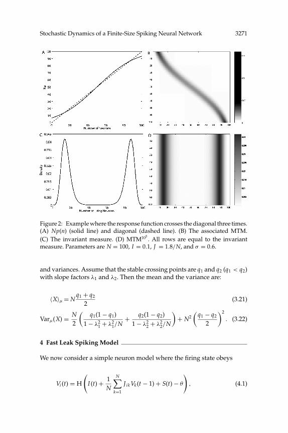
3.3 Multiple Crossing Points. For dynamics where 0 < p < 1, if theresponse function is continuous and crosses the diagonal more than once,then the number of crossings must be odd. Consider the case with threecrossings with p(0) < p(N). If the slopes of all the crossings are positive(i.e., a sigmoidal response function), then the slope factor λ of the middlecrossing will be greater than one, and the other two crossings will have λ lessthan one, implying two stable crossing points and one unstable one in themiddle. Figures 2A and 2B provide an example of such a response functionand its associated MTM. The invariant measure is shown in Figure 2C. Wesee that it is bimodal with local peaks at the two crossing points with λ

less than one. The invariant measure is well approximated by any row ofa large power of the MTM (see Figure 2D). If the stable crossing pointsare separated enough (beyond a few standard deviations), then we canestimate the network mean and variance by combining the two local mean


Figure 2: Example where the response function crosses the diagonal three times.(A) Np(n) (solid line) and diagonal (dashed line). (B) The associated MTM.(C) The invariant measure. (D) MTM105

. All rows are equal to the invariantmeasure. Parameters are N = 100, I = 0.1, J = 1.8/N, and σ = 0.6.

and variances. Assume that the stable crossing points are q1 and q2 (q1 < q2)with slope factors λ1 and λ2. Then the mean and the variance are:

〈X〉µ = Nq1 + q2

2(3.21)

Varµ(X) = N2

(q1(1 − q1)

1 − λ21 + λ2

1/N+ q2(1 − q2)

1 − λ22 + λ2

2/N

)+ N2

(q1 − q2

2

)2

. (3.22)

4 Fast Leak Spiking Model

We now consider a simple neuron model where the firing state obeys

Vi (t) = H

(I (t) + 1

N

N∑k=1

J ik Vk(t − 1) + S(t) − θ

), (4.1)


where H(·) is the Heaviside step function, I (t) is an input current, S(t) =N(0, σ ) is uncorrelated gaussian noise, θ is a threshold, and J ik is the connec-tion strength between neurons in the network. When the combined inputof the neuron is below threshold, Vi = 0 (neuron is silent), and when theinput exceeds threshold, Vi = 1 (neuron is active). This is a simple versionof a spike response or renewal model (Gerstner & van Hemmen, 1992;Gerstner, 1995; Meyer & Van Vreeswijk, 2002).

In order to apply our Markov formalism, we need to construct the re-sponse function. We assume first that the connection matrix has constantentries J . We will also consider disordered connectivity later. The responsefunction is the probability that a neuron will fire given that n neurons firedpreviously. The response function at t for the neuron is then given by

p(n, t) = 1√2π

∫ ∞

θ−I (t)−nJ /Nσ

e−x2/2dx. (4.2)

If we assume a time-independent input, then we can construct the MTMusing equation 2.2. The equilibrium PDF is given by equation 3.1 and canbe approximated by one row of a large power of the MTM.

4.1 Mean, Variance, and Autocorrelation. Imposing the self-consistency condition, equation 3.10, on the mean activity Nq , whereq = 〈p〉µ, and p is given by equation 4.2 leads to

q = 1√2π

∫ ∞

θ−I−q Jσ

e−x2/2dx. (4.3)

Taking the derivative of p(n, t) in equation 3.10 at n = Nq gives

λ = J

σ√

2πe− (θ−I−J q )2

2σ2 . (4.4)

Using this in equation 3.17 gives the variance.Equation 4.4 shows the influence of noise and recurrent excitation on

the slope factor and hence variance of the network activity. For λ < 1, thevariance 3.17 increases with λ. An increase in excitation J increases λ forlarge J but decreases λ for small J . Similarly, a decrease in noise σ increasesλ for large σ but decreases it for small σ . Thus, variability in the system canincrease or decrease with synaptic excitation and external noise dependingon the regime. The autocovariance function, from equation 3.20, is

Cov(τ ) = λτ Nq (1 − q )1 − λ2 + λ2/N

. (4.5)


4.2 Bifurcation Diagram. Bifurcations occur when the stability of themean field solutions (i.e., crossing points) for the mean activity changes.We can construct the bifurcation diagram on the I − J plane by locatingcrossing points where λ = 1. We first consider rescaled parameters I =(θ − I )/σ and J = J /σ . Then equation 4.3 becomes

q = 1√2π

∫ ∞

I−qJe−x2/2dx, (4.6)

and equation 4.4 becomes

λ = J√2π

e− (I−J q )2

2 . (4.7)

Solving equation 4.7 for q and inserting into equation 4.6 gives

I = J√2π

∫ ∞

±√

ln( J 2

2πλ2 )e−x2/2dx ±

√ln

( J 2

2πλ2

). (4.8)

The bifurcation points are obtained by setting λ = 1 in equation 4.8and evaluating the integral. The solutions have two branches that sat-isfy the conditions J ≥ √

2π and I ≥ √π/2. Figure 3A shows the two-

dimensional bifurcation diagram on the I − J plane. The intersection ofthe two branches at J = √

2π and I = √π2 is a codimension two cusp bifur-

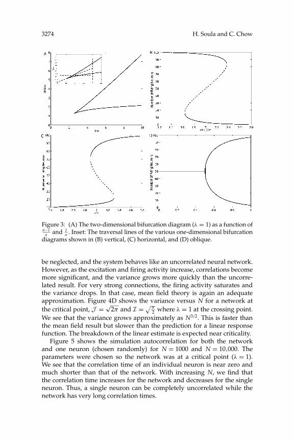
cation point (i.e., satisfies Np′(x) = 1, Np′′(x) = 0 with genericity conditions;Kuznetsov, 1998). Between the two branches are three crossing points (twoof which are stable), and outside there is one stable crossing point. Eachtraversal of a branch yields a saddle node bifurcation as seen in Figures3B and 3C for the vertical and horizontal traversals (shown in the insetto Figure 3A), respectively. Traversing through the critical point along thediagonal line in the inset of Figure 3A shows a pitchfork bifurcation. Wehave assumed that J > 0 (i.e., excitatory network). By taking J → −J , weobtain the same bifurcation diagram for the inhibitory case, and the aboveconditions still hold using the absolute value of J .

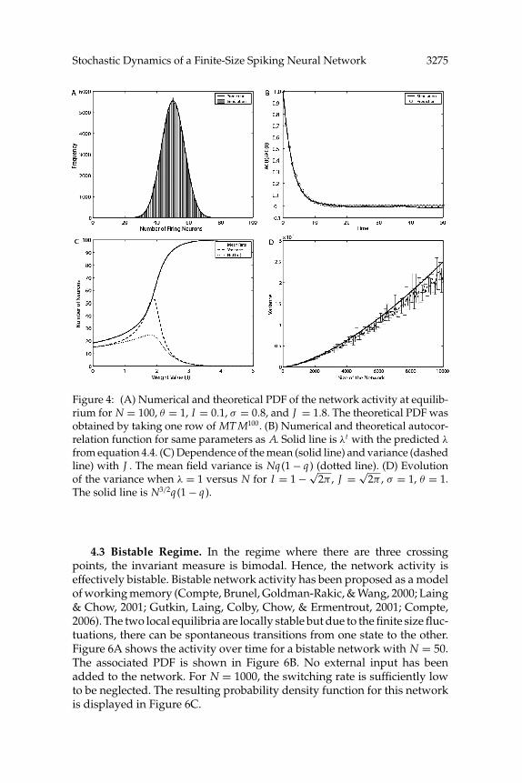
We compare our analytical estimates from the Markov model with nu-merical simulations of the fast leak model 4.1 in Figure 4. Figure 4A showsthat the equilibrium PDF derived from the MTM matches the PDF generatedfrom the simulation. Figure 4B shows a comparison of λτ versus the simula-tion autocorrelation function. Figure 4C shows the mean and variance of theactivity versus the connection weight J . The theoretical results match thesimulation results very well. On the same plot, we show the mean field the-ory estimate where the neurons are assumed to be completely uncorrelated.For low recurrent excitation and, hence, low activity, the correlations can


Figure 3: (A) The two-dimensional bifurcation diagram (λ = 1) as a function ofθ−Iσ

and Jσ

. Inset: The traversal lines of the various one-dimensional bifurcationdiagrams shown in (B) vertical, (C) horizontal, and (D) oblique.

be neglected, and the system behaves like an uncorrelated neural network.However, as the excitation and firing activity increase, correlations becomemore significant, and the variance grows more quickly than the uncorre-lated result. For very strong connections, the firing activity saturates andthe variance drops. In that case, mean field theory is again an adequateapproximation. Figure 4D shows the variance versus N for a network atthe critical point, J = √

2π and I = √π2 where λ = 1 at the crossing point.

We see that the variance grows approximately as N3/2. This is faster thanthe mean field result but slower than the prediction for a linear responsefunction. The breakdown of the linear estimate is expected near criticality.

Figure 5 shows the simulation autocorrelation for both the networkand one neuron (chosen randomly) for N = 1000 and N = 10,000. Theparameters were chosen so the network was at a critical point (λ = 1).We see that the correlation time of an individual neuron is near zero andmuch shorter than that of the network. With increasing N, we find thatthe correlation time increases for the network and decreases for the singleneuron. Thus, a single neuron can be completely uncorrelated while thenetwork has very long correlation times.


Figure 4: (A) Numerical and theoretical PDF of the network activity at equilib-rium for N = 100, θ = 1, I = 0.1, σ = 0.8, and J = 1.8. The theoretical PDF wasobtained by taking one row of MT M100. (B) Numerical and theoretical autocor-relation function for same parameters as A. Solid line is λt with the predicted λ

from equation 4.4. (C) Dependence of the mean (solid line) and variance (dashedline) with J . The mean field variance is Nq (1 − q ) (dotted line). (D) Evolutionof the variance when λ = 1 versus N for I = 1 − √

2π , J = √2π , σ = 1, θ = 1.

The solid line is N3/2q (1 − q ).

4.3 Bistable Regime. In the regime where there are three crossingpoints, the invariant measure is bimodal. Hence, the network activity iseffectively bistable. Bistable network activity has been proposed as a modelof working memory (Compte, Brunel, Goldman-Rakic, & Wang, 2000; Laing& Chow, 2001; Gutkin, Laing, Colby, Chow, & Ermentrout, 2001; Compte,2006). The two local equilibria are locally stable but due to the finite size fluc-tuations, there can be spontaneous transitions from one state to the other.Figure 6A shows the activity over time for a bistable network with N = 50.The associated PDF is shown in Figure 6B. No external input has beenadded to the network. For N = 1000, the switching rate is sufficiently lowto be neglected. The resulting probability density function for this networkis displayed in Figure 6C.


Figure 5: Autocorrelation of the network and one neuron at a critical point(λ = 1). The solid line is for a network of 10,000 neurons and the dashed line isfor a network of 1000 neurons. Crosses and dots are the autocorrelation of oneneuron for N = 1000 and N = 10,000, respectively. The autocorrelation for oneneuron decays almost immediately. Parameters are σ = 1, θ = 1, J = √

2π , andI = 1 − √

2/π .

We can estimate the scaling behavior on N of the state switching rate,and hence lifetime of a memory, by supposing the finite-size induced fluc-tuations can be approximated by uncorrelated gaussian noise. We can thenmap the switching dynamics to barrier hopping of a stochastically forcedparticle in a double potential well V(x) with a stationary PDF given by theinvariant measure µ. The switching rate is given by the formula (Risken,1989)

r = (2π)−1√

V′′(c)|V′′(a )|e− (V(a )−V(c))σ2 , (4.9)

where V = −σ 2 ln(µ), µ is the invariant measure, c is a stable crossing point,a is the unstable crossing point, and σ 2 is the forcing noise variance aroundc, which we take to be proportional to the variance of the network activity.For the general case, we cannot derive this rate analytically, but we can


Figure 6: (A) The firing activity over time of a bistable network of 50 neurons.The switching between the two states (high and low activity) is spontaneous.(B) Theoretical PDF for N = 50. (C) Theoretical PDF for N = 1000. (D) Switchingrate depends exponentially on N (solid curve). The dashed line is a linear fit ona semilog scale. Parameters are J = 1.8, σ = 0.6, I = 0.1, and θ = 1.

obtain an estimate by assuming that the invariant measure is a sum of twogaussian PDFs whose means are exactly the two stable crossing points:

µ(x) =exp

(− (x−Nq1)2

2σ 21

)2√

2πσ1+

exp(− (x−Nq2)2

2σ 22

)2√

2πσ2, (4.10)

where σ 2i = Nqi (1−qi )

1−λ2i +λ2

i /Nfor i = 1, 2. Using this in equation 4.9 then gives

r ∝ �e−k N (4.11)

for a constant k. The switching rate is an exponentially decreasing functionof N. We computed the switching rate for N ∈ [0; 150] for the parametersof the bistable network above. The results are displayed in Figure 6D. Forthe parameters in Figure 6D, a fit shows that k is of order 0.05. For these


parameters, switching between states will not be important when N �1/k ∼ 20.

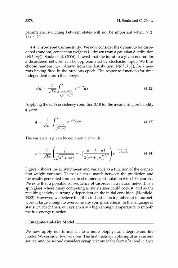
4.4 Disordered Connectivity. We now consider the dynamics for disor-dered (random) connection weights J i j drawn from a gaussian distribution(N( J , σ 2

J )). Soula et al. (2006) showed that the input to a given neuron fora disordered network can be approximated by stochastic input. We thuschoose random input drawn from the distribution, N(k J , kσ 2

J ), for k neu-rons having fired in the previous epoch. The response function (for timeindependent input) then obeys

p(n) = 1√2π

∫ ∞

θ−I−nJ /N√σ2+nσ2

J /N

e−x2/2dx. (4.12)

Applying the self-consistency condition 3.10 for the mean firing probabilityq gives

q = 1√2π

∫ ∞

θ−I−q J√σ2+qσ2

J

e−x2/2dx. (4.13)

The variance is given by equation 3.17 with

λ = 1√2π

J√

σ 2 + qσ 2J

− σ 2J

θ − I − q J

2(σ 2 + qσ 2

J

)3/2

e

− (θ−I− J q )2

2(σ2+qσ2J ) . (4.14)

Figure 7 shows the activity mean and variance as a function of the connec-tion weight variance. There is a close match between the prediction andthe results generated from a direct numerical simulation with 100 neurons.We note that a possible consequence of disorder in a neural network is aspin glass where many competing activity states could coexist, and so theresulting activity is strongly dependent on the initial condition (Hopfield,1982). However, we believe that the stochastic forcing inherent in our net-work is large enough to overcome any spin glass effects. In the language ofstatistical mechanics, our system is at a high enough temperature to smooththe free energy function.

5 Integrate-and-Fire Model

We now apply our formalism to a more biophysical integrate-and-firemodel. We consider two versions. The first treats synaptic input as a currentsource, and the second considers synaptic input in the form of a conductance


Figure 7: Mean (crosses) and variance (diamonds) from a numerical simulationof the fast leak model for N = 100 neurons as a function of the variance ofthe random disordered connection weights. Theoretical mean (solid line) andvariance (dashed line) match well with numerical simulation values. Parametersare J = 0.5/N, I = 0.1, σ = 1.0, and θ = 1.0.

change. We apply our Markov model with a discrete time step chosen to bethe larger of the membrane or synaptic time constants.

5.1 Current-Based Synapse. We first consider an integrate-and-firemodel where the synaptic input is applied as a current. The membranepotential obeys

τdv

dt= I − V + J

N

N∑t f <t

α(t − t f ) + Z(t), (5.1)

where α(t) = e− tτs /τs if t > 0 and zero otherwise, I is a constant input, Z is

an uncorrelated zero-mean white noise with variance σ , J is the synapticstrength coefficient, N is the network size, and t f are the firing times ofall neurons in the network. These firing times are computed whenever themembrane potential crosses a threshold Vθ , whereupon the potential is resetto VRs . After firing, neurons are prevented from firing during an absolute


refractory period r . The parameter values are τ = 1 ms, τs = 1 ms,Vr =−65 mV, Vθ = −60 mV, VRs = −80 mV, and r = 1 ms.

The network dynamics of this model were studied previously in detailwith a Fokker-Planck formalism (Brunel, 2000; Brunel & Hansel, 2006).These analyses showed that if the input current is an uncorrelated whitenoise N(µI , σ

2I ) and τs < 1, then the response function of the neuron in

equilibrium is given by

1p(X)

= r + √π

∫ Vθ −µI −J X/N

σ2I

Vr −µI −J X/N

σ2I

dueu2(1 + erf (u)). (5.2)

The mean activity is again given by Nq where 〈p(X)〉µ = q , and q is asolution of equation 3.10:

q =r + √

π

∫ Vθ −µI −J q

σ2I

Vr −µI −J q

σ2I

dueu2(1 + er f (u))

−1

. (5.3)

Using equation 5.3, we can derive the slope factor λ,

λ = m2 Jσ 2

I

e

(Vθ −µI −J m

σ2I

)2 (1 + er f

(Vθ − µI − Jm

σ 2I

))

−e

(Vr −µI −J m

σ2I

)2 (1 + er f

(Vr − µI − Jm

σ 2I

)) , (5.4)

which can be used to estimate the variance using equation 3.17.We also evaluate the response function numerically. We assume that the

response function can be approximated by the firing probability of a neuronwhose membrane potential obeys

τdVdt

= I + J XN

− V(t) + Z(t), (5.5)

where X ∈ {0, . . . , N}. This presumes that the effect of discrete synapticevents can be approximated by a constant input equivalent to the meaninput plus noise. We estimated the firing probability in a temporal epochfrom the average firing rate of the neuron obeying equation 5.5 for eachX. We used the firing probabilities directly to form the MTM. We thencomputed the equilibrium PDF, the mean activity (crossing point), the slope


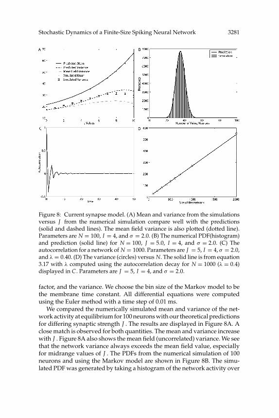
Figure 8: Current synapse model. (A) Mean and variance from the simulationsversus J from the numerical simulation compare well with the predictions(solid and dashed lines). The mean field variance is also plotted (dotted line).Parameters are N = 100, I = 4, and σ = 2.0. (B) The numerical PDF(histogram)and prediction (solid line) for N = 100, J = 5.0, I = 4, and σ = 2.0. (C) Theautocorrelation for a network of N = 1000. Parameters are J = 5, I = 4, σ = 2.0,and λ = 0.40. (D) The variance (circles) versus N. The solid line is from equation3.17 with λ computed using the autocorrelation decay for N = 1000 (λ = 0.4)displayed in C . Parameters are J = 5, I = 4, and σ = 2.0.

factor, and the variance. We choose the bin size of the Markov model to bethe membrane time constant. All differential equations were computedusing the Euler method with a time step of 0.01 ms.

We compared the numerically simulated mean and variance of the net-work activity at equilibrium for 100 neurons with our theoretical predictionsfor differing synaptic strength J . The results are displayed in Figure 8A. Aclose match is observed for both quantities. The mean and variance increasewith J . Figure 8A also shows the mean field (uncorrelated) variance. We seethat the network variance always exceeds the mean field value, especiallyfor midrange values of J . The PDFs from the numerical simulation of 100neurons and using the Markov model are shown in Figure 8B. The simu-lated PDF was generated by taking a histogram of the network activity over


105 ms. For the Markov model, the PDF is the eigenvector with eigenvalueone and approximated by taking a single row of the one-hundredth powerof the MTM.

The model predicts an exponentially decaying autocorrelation functionwith time constant 1/ ln(λ). It is displayed in Figure 8C for a network ofN = 1000. We used the same parameters as in Figure 8A with a connectionweight where the dynamics deviates from mean field theory (J = 5). In thisparameter range, the recurrent excitation is strong, and the single-neuronfiring rate is very high—approximately 350 Hz (the refractory time of 1 msimposes a maximum frequency is 1000 Hz). In this regime, the refractorytime acts like inhibition, so the probability of firing actually decreases if theactivity in the previous epoch increases. Thus, the autocorrelation functionexhibits anticorrelations as seen in the Figure 8C. We can estimate λ byfitting the autocorrelation to λτ . Using the approximation λ = Cov(1)/Vargives |λ| = 0.40. The theoretical value of |λ| using equation 5.4 gives 0.37 forthe same parameters (using the simulated mean number of firing neurons).Figure 8D shows a plot of the variance versus N for the numerical simu-lation. The simulated variance is well matched by the estimated variancefrom equation 3.17 with q measured from the simulation (estimated by themean firing rate of a single neuron) and λ = 0.4.

5.2 Conductance-Based Synapse. We now consider the integrate-and-fire neuron model with conductance-based synaptic connections. The mem-brane potential V obeys

τdVdt

= I (t) − (V − Vr ) − s(t) (V − Vs) + Z(t), (5.6)

where τ is the membrane time constant, I (t) is an input current, Z(t) iszero-mean white noise with variance σ , Vr is the rest potential, and Vs isthe reversal potential of an excitatory synapse. The synaptic gating variables(t) obeys

τsdsdt

= JN

∑t f

δ(t − t f ) − s(t), (5.7)

where τs is the synaptic time constant, J is the maximal synaptic conduc-tance, N is the number of neurons in the network, and t f are the firing timesof all neurons in the network. The threshold is Vθ , and the reset potentialis VR. As with the previous model, a refractory period r was introduced.We used τ = 1 ms, τs = 1 ms, Vr = −65 mV, Vs = 0 mV, Vθ = −60 mV,VR = −80 mV, τs = 1 ms, and r = 1 ms.


Figure 9: Conductance synapse model. (A) Mean and variance from the simula-tions versus J from the numerical simulation compare well with the predictions(solid and dashed lines). Parameters are N = 100, I = 4, and σ = 2.0. (B) The nu-merical PDF(histogram) and prediction (solid line) for N = 100, I = 4, σ = 2.0,and J = 0.05. (C) The autocorrelation for a network of N = 1500. Parametersare J = 0.05, I = 4, σ = 2.0, and λ = 0.31. (D) The variance (circles) versus N.The solid line is from equation 3.17 with λ computed using the autocorrelationdecay for N = 1500 (λ = 0.31) displayed in C . Parameters are J = 0.05, I = 4,and σ = 2.0.

We computed the response function by measuring numerically the firingprobability of a neuron that obeys

τdVdt

= I − (V − Vr ) − J XN

(V − Vrvs) + Z(t) (5.8)

for all X ∈ {0, . . . , N} using the same method as in the current-based model.From the response function, we obtained the MTM and the invariant mea-sure. Figure 9A compares the mean and variance of a numerical simulationwith the Markov prediction for varying J . We see that there is a good match.For J = 0.05, we compare the numerically computed PDF with the invari-ant measure. As shown in Figure 9B, the prediction is extremely accurate.


We estimated the slope factor as in the previous section using the auto-correlation function for N = 1500 and found λ = 0.31 and computed theestimated variance for various N. The comparison is shown on Figure 9D.There is again a close match.

6 Discussion

Our model relies on the assumption that the neuronal dynamics can berepresented by a Markov process. We partition time into discrete epochs,and the probability that a neuron will fire in one epoch depends on onlythe activity of the previous epoch. For this approximation to be valid, atleast two conditions must be met. The first is that the epoch time needsto be long enough so that the influence of activity in the distant past isnegligible. The second is that the epoch time needs to be short enough sothat a neuron fires at most once within an epoch. The influence time of aneuron is given approximately by the larger of the membrane time constant(τm) and synaptic time constant (τs). Presumably the neuron does not havea memory of events much beyond this timescale. This gives a lower boundon the epoch time �t. Hence, �t > max[τm, τs]. The second condition isequivalent to f �t < 1, where f is the maximum firing rate of a neuron inthe network. Thus, the Markov model is applicable for

max[τm, τs] < f −1. (6.1)

This condition is not too difficult to satisfy. For example, a cortical neuronreceiving AMPA inputs with a membrane time constant less than 20 mscan satisfy the Markov condition if its maximum firing rate is below 50 Hz.Since typical cortical neurons have a membrane time constant between1 and 20 ms and many recordings in the cortex find rates below 50 Hz(Nicholls, Martin, & Wallace, 1992), our formalism could be applicable to abroad class of cortical circuits.

The equilibrium state of our Markov model exists and is exactly solvableif the response function is never zero or one. In other words, a neuron in thenetwork always has a nonzero probability of firing but never has full cer-tainty it will fire. Hence, the neuronal dynamics are always fully stochastic.Thus, the equilibrium state of a fully stochastic network could be anotherdefinition of the asynchronous state. However, although the network iscompletely stochastic, the activity is not uncorrelated. These correlationsare manifested in the entire network activity but not within the firing statis-tics of the individual neurons, which obey a simple random binomial orPoisson distribution. The autocorrelation function of the individual neuronalso decays much more quickly than that of the network.

Many previous approaches to studying the asynchronous state as-sumed that neuronal firing was statistically independent so a mean field


description was valid. With our simple model, we can compute the equilib-rium PDF directly and explicitly determine the parameter regimes wheremean field theory breaks down. We also show that the order parameterthat determines nearness to criticality is the slope of the response functionaround the equilibrium mean activity. As expected, we find that mean fieldtheory is less applicable for small or strongly recurrent neural circuits. Inour model, the mean activity of our network can be obtained using meanfield theory except at the critical point. We compute the variance of thenetwork activity directly and see precisely how the network dynamics de-viate from mean field theory as we approach the critical point. We notethat while our closed-form estimates for the mean and variance may breakdown very near criticality, our model does not. The invariant measure ofthe MTM still gives the equilibrium PDF and in principle can be computedto arbitrary precision. Hence, our model can serve as a simple example ofwhen mean field theory is applicable. We note that even in the limit of Ngoing to infinity, the variance of the network deviates from a network ofindependent neurons by a factor of (1 − λ)−1. The deviations from meanfield theory persist even in an infinite-sized network.

Our model requires statistical homogeneity. While purely homogeneousnetworks are unrealistic for biological networks, statistical homogeneitymay be more plausible. For some classes of inputs, the probability of firingfor a given set of neurons could be uniform over some limited temporalduration. We found that our analytical estimates can be modified to ac-count for disordered randomness in the connections. A model that fullyincorporated all heterogeneous effects would require taking into accountdifferent populations. However, with each additional population, the di-mension of the MTM increases by a power of N. Thus, for a network of twopopulations, say inhibitory and excitatory neurons, the resulting problemwill involve an MTM with N2 × N2 elements.

Future work could examine the behavior at the critical point more care-fully. Our variance estimate predicted that the variance at criticality woulddiverge as the system size squared, but simulations found an exponent of3/2. We also showed that the correlation time of the network activity di-verged at the critical point. We expect correlations to obey a power law atcriticality. Perhaps a renormalization group approach may be adapted tostudy the scaling behavior near criticality. Recent experiments have foundthat cortical slices exhibit critical behavior (Beggs & Plenz, 2003, 2004). OurMarkov model may be an ideal system to explore critical behavior.

Finally, we note that even at the critical point, where the network activityis highly correlated, the single-neuron dynamics can exhibit uncorrelatedPoisson statistics. This shows that collective network dynamics may not bededucible from single-neuron dynamics. Using our model as a basis, it maybe possible to probe characteristics about local network size, connectivity,and nearness to criticality by combining recordings of single neurons withmeasurements of the local field potential.


Appendix A: Mean and Variance Derivations

The mean activity is given by

〈X〉t =N∑

k=0

k Pk(t)

=N∑

k=0

kN∑

i=0

CkN(1 − pi )N−k pk

i Pi (t − 1).

Rearranging yields

〈X〉t =N∑

i=0

Pi (t − 1)N∑

k=0

kCkN(1 − pi )N−k pk

i .

Since∑N

k=0 kCkN(1 − pi )N−k pk

i = Npi is the mean of a binomial distribution,we obtain

〈X〉t =N∑

i=0

Pi (t − 1)Npi

= N〈p〉t−1

which is equation 3.4.The variance is given by

Vart(X) =N∑

k=0

k2 Pk(t) − N2〈p〉2t−1

=N∑

k=0

k2N∑

i=0

CkN(1 − pi )N−k pk

i Pi (t − 1) − N2〈p〉2t−1

=N∑

i=0

Pi (t − 1)N∑

k=0

k2CkN(1 − pi )N−k pk

i − N2〈p〉2t−1

=N∑

i=0

Pi (t − 1)Npi (1 − pi ) +N∑

i=0

Pi (t − 1)N2 p2i − N2〈p〉2

t−1

= N〈p(1 − p)〉t−1 + N2Vart−1(p),


where we have used the variance of a binomial distribution Np(1 − p). Forthe linear case, writing p(X) = a + b X we have:

Varµ(X) = N〈p(1 − p)〉µ + N2〈p2〉µ − N2〈p〉2µ

= N〈a + b X − a2 − 2ab X − b2 X2〉µ + N2〈a2 + 2ab X + b2 X2〉µ− N2〈a + b X〉2

µ

= Na + b N〈X〉 − Na2 − 2Nab〈X〉 − Nb2〈X2〉 + N2a2 + 2N2ab〈X〉+ N2b2〈X2〉 − N2(a2 + 2ab〈X〉 + b2〈X〉2)

= Na − Na2 + N2a2 − N2a2 + 〈X〉(b N − 2Nab + 2N2ab − 2N2ab)

+ 〈X2〉(−Nb2 + N2b2) − b2 N2〈X〉2

= Na − Na2 + b N(1 − 2a )〈X〉 + (N2b2 − Nb2)Var(X) − Nb2〈X〉2

= Na − Na2 + b N(1 − 2a )〈X〉 − Nb2〈X〉2

1 − N2b2 + Nb2 .

Setting a = p0 and b = (q−p0)Nm gives

Varµ(X) = q 2 Np0(1 − p0) + (q − p0)(1 − p0 − q )

q 2 − (q − p0)2 + (q − p0)2/N.

If we set λ = (q − p0)/q , we get equation 3.17.

Appendix B: Autocovariance Function

We prove the form of the autocovariance function Cov(τ ) = λτ Varµ(X) forthe linear response function using induction. We first show that Cov(1) =λVarµ(X) and then Cov(τ + 1) = λCov(τ ).

The autocovariance function when τ = 1 is given by

Cov(1) = 〈Xt Xt+1〉 − 〈X〉2µ

=N∑

k=0

N∑i=0

ki P(Xt+1 = i |Xt = k)P(Xt = k) − 〈X〉2µ

= NN∑

k=0

kpk P(Xt = k) − 〈X〉2µ

= N〈pX〉µ − 〈X〉2µ.


For a linear response function p, we obtain

Cov(1) = N〈pX〉µ − 〈X〉2µ

= N⟨

p0 X + q − p0

NqX2

⟩µ

− N2m2

= N2 p0q +⟨

q − p0

qX2

⟩µ

− N2q 2

= N2q (p0 − q ) + q − p0

q

(Varµ(X) + N2q 2)

= q − p0

qVarµ(X).

Hence for τ = 1, the autocovariance function is equal to the slope factorλ = (q − p0)/q times the variance. Assume for τ that Cov(τ ) = λτ Varµ(X);then

Cov(τ + 1) =〈Xt Xt+τ+1〉 − 〈X〉2µ

=N∑

k=0

N∑j=0

k j P(Xt = k)P(Xt+τ+1 = j |Xt = k) − 〈X〉2µ

=N∑

k=0

N∑j=0

k j P(Xt = k)N∑

r=0

P(Xt+τ+1 = j |Xt+τ = r )P

× (Xt+τ = r |Xt = k) − 〈X〉2µ

=N∑

k=0

N∑j=0

N∑r=0

k j P(Xt = k)C jN(1 − p(r ))N− j p(r ) j P

× (Xt+τ = r |Xt = k) − 〈X〉2µ

=N∑

k=0

N∑r=0

Nkp(r )P(Xt = k)P(Xt+τ = r |Xt = k) − 〈X〉2µ,

using the mean of the binomial distribution. We can now insert the linearresponse function to obtain

Cov(τ + 1) =N∑

k=0

N∑r=0

Nk(

p0 + q − p0

Nqr)

P(Xt = k)P(Xt+τ = r |Xt = k)−〈X〉2µ


=N∑

k=0

N∑r=0

Nkp0 P(Xt = k)P(Xt+τ = r |Xt = k)

+ q − p0

q

(Cov(τ )〈X〉2

µ

) − 〈X〉2µ

because

N∑k=0

N∑r=0

kr P(Xt = k)P(Xt+τ = r |Xt = k) = Cov(t + τ ) + 〈X〉2µ.

Then since

N∑k=0

N∑r=0

Nkp0 P(Xt = k)P(Xt+τ = r |Xt = k) =N∑

k=0

Nkp0 P(Xt = k),

because

N∑r=0

P(Xt+τ = r |Xt = k) = 1,

for all k and

N∑k=0

Nkp0 P(Xt = k) = 〈Np0 X〉µ = N2 p0q ,

we finally obtain

Cov(τ + 1) = N2 p0q + q − p0

q〈X〉2

µ − 〈X〉2µ + λCov(τ )

= N2 p0q + q − p0

qN2q 2 − N2q 2 + λCov(τ )

= N2(p0q + (q − p0)q − q 2) + λCov(τ )

= λCov(τ ).

proving equation 3.20 by induction.

Acknowledgments

This work was supported by the Intramural Research Program of NIH,NIDDK. We thank Michael Buice for his helpful comments on themanuscript.


References

Abbott, L., & Van Vreeswijk, C. (1993). Asynchronous states in a network of pulse-coupled oscillators. Phys. Rev. E, 48(2), 1483–1490.

Amit, D. J., & Brunel, N. (1997a). Dynamics of recurrent spiking neurons before andfollowing learning. Network: Comput. Neural. Syst., 8, 373–404.

Amit, D. J., & Brunel, N. (1997b). Model of global spontaneous activity and localstructured activity during delay periods in the cerebral cortex. Cereb. Cortex, 7(3),237–252.

Beggs, J. M., & Plenz, D. (2003). Neuronal avalanches in neocortical circuits. J. Neu-rosci., 23(35), 11167–11177.

Beggs, J. M., & Plenz, D. (2004). Neuronal avalanches are diverse and precise activitypatterns that are stable for many hours in cortical slice cultures. J. Neurosci., 24(22),5216–5229.

Brunel, N. (2000). Dynamics of sparsely connected networks of excitatory and in-hibitory spiking neurons. J. Comput. Neurosci., 8(3), 183–208.

Brunel, N. (2003). Dynamics and plasticity of stimulus-selective persistent activityin cortical network models. Cereb. Cortex, 13(11), 1151–1161.

Brunel, N., & Hansel, D. (2006). How noise affects the synchronization properties ofrecurrent networks of inhibitory neurons. Neural Comput., 18(5), 1066–1110.

Cai, D., Tao, L., Shelley, M., & McLaughlin, D. W. (2004). An effective kinetic rep-resentation of fluctuation-driven neuronal networks with application to simpleand complex cells in visual cortex. Proc. Natl. Acad. Sci. USA, 101(20), 7757–7762.

Compte, A. (2006). Computational and in vitro studies of persistent activity: Edgingtowards cellular and synaptic mechanisms of working memory. Neuroscience,139(1), 135–151.

Compte, A., Brunel, N., Goldman-Rakic, P. S., & Wang, X. J. (2000). Synaptic mech-anisms and network dynamics underlying spatial working memory in a corticalnetwork model. Cereb. Cortex, 10(9), 910–923.

Del Giudice, P., & Mattia, M. (2003). Stochastic dynamics of spiking neurons. InE. Korutcheva & K. Cureno (Eds.), Advances in condensed matter and statisticalphysics (pp. 125–153). Hauppauge, NY: Nova Science.

Fourcaud, N., & Brunel, N. (2002). Dynamics of the firing probability of noisyintegrate-and-fire neurons. Neural Comput., 14(9), 2057–2110.

Fries, P., Reynolds, J. H., Rorie, A. E., & Desimone, R. (2001). Modulation of oscillatoryneuronal synchronization by selective visual attention. Science, 291(5508), 1560–1563.

Fusi, S., & Mattia, M. (1999). Collective behavior of networks with linear (VLSI)integrate-and-fire neurons. Neural Comput., 11, 633–652.

Gerstner, W. (1995). Time structure of the activity in neural network models. PhysicalReview E: Statistical Physics, Plasmas, Fluids, and Related Interdisciplinary Topics,51(1), 738–758.

Gerstner, W. (2000). Population dynamics of spiking neurons: Fast transients, asyn-chronous states and locking. Neural Comput., 12, 43–89.

Gerstner, W., & van Hemmen, J. (1992). Associative memory in a network of“spiking” neurons. Network, 3, 139–164.


Gerstner, W., & Kistler, W. (2002). Spiking neuron models—single neurons, populations,plasticity. Cambridge: Cambrige University Press.

Ginzburg, I., & Sompolinsky, H. (1994). Theory of correlations in stochastic neuralnetworks. Phys. Rev. E.: Stat. Nonlin. Soft Matter Phys., 50(4), 3171–3191.

Golomb, D., & Hansel, D. (2000). The number of synaptic inputs and the synchronyof large, sparse neuronal networks. Neural Computation, 12(5), 1095–1139.

Gutkin, B. S., Laing, C. R., Colby, C. L., Chow, C. C., & Ermentrout, G. B. (2001).Turning on and off with excitation: The role of spike-timing asynchrony andsynchrony in sustained neural activity. J. Comput. Neurosci., 11(2), 121–134.

Hansel, D., & Mato, G. (2003). Asynchronous states and the emergence of synchronyin large networks of interacting excitatory and inhibitory neurons. Neural Com-put., 15(1), 1–56.

Hopfield, J. J. (1982). Neural networks and physical systems with emergent compu-tational properties. Proc. Natl. Acad. Sci. USA, 79(2), 2554–2558.

Kuznetsov, Y. (1998). Elements of bifurcation theory (2nd ed.). Berlin: Springer.Laing, C. R., & Chow, C. C. (2001). Stationary bumps in networks of spiking neurons.

Neural Comput., 13(7), 1473–1494.Mattia, M., & Del Giudice, P. (2002). Population dynamics of interacting spiking

neurons. Physical Review E, 66(5), 051917.Meyer, C., & Van Vreeswijk, C. (2002). Temporal correlations in stochastic networks

of spiking neurons. Neural Computation, 14(2), 369–404.Nicholls, J., Martin, A., & Wallace, B. (1992). From neuron to brain (3rd ed.).

Sunderland, MA: Sinauer Associates.Nykamp, D., & Tranchina, D. (2000). A population density approach that facilitates

large-scale modeling of neural networks: Analysis and an application to orienta-tion tuning. Journal of Computational Neuroscience, 8, 19–50.

Pesaran, B., Pezaris, J. S., Sahani, M., Mitra, P. P., & Andersen, R. A. (2002). Tempo-ral structure in neuronal activity during working memory in macaque parietalcortex. Nat. Neurosci., 5(8), 805–811.

Plesser, H. E., & Gerstner, W. (2000). Noise in integrate-and-fire models: Fromstochastic input to escape rates. Neural Computation, 12, 367–384.

Risken, H. (1989). The Fokker-Planck equation: Methods of solution and application (2nded.). Berlin: Springer.

Salinas, E., & Sejnowski, T. J. (2002). Integrate-and-fire neurons driven by correlatedstochastic input. Neural Comput., 14(9), 2111–2155.

Seung, H. S. (1996). How the brain keeps the eyes still. Proc. Natl. Acad. Sci. USA,93(23), 13339–13344.

Singer, W., & Gray, C. M. (1995). Visual feature integration and the temporal corre-lation hypothesis. Annu. Rev. Neurosci., 18, 555–586.

Softky, W. R., & Koch, C. (1993). The highly irregular firing of cortical cells is in-consistent with temporal integration of random EPSPS. J. Neurosci., 13(1), 334–350.

Soula, H., Beslon, G., & Mazet, O. (2006). Spontaneous dynamics of asymmetricrandom recurrent spiking neural networks. Neural Computation, 18(1), 60–79.

Steinmetz, P. N., Roy, A., Fitzgerald, P. J., Hsiao, S. S., Johnson, K. O., & Niebur, E.(2000). Attention modulates synchronized neuronal firing in primate somatosen-sory cortex. Nature, 404(6774), 187–190.


Treves, A. (1993). Mean-field analysis of neuronal spike dynamics. Network, 4, 259–284.

Van Vreeswijk, C., & Sompolinsky, H. (1996). Chaos in neuronal networks withbalanced excitatory and inhibitory activity. Science, 274, 1724–1726.

Van Vreeswijk, C., & Sompolinsky, H. (1998). Chaotic balanced state in a model ofcortical circuits. Neural Comput., 10(6), 1321–1371.

Received August 9, 2006; accepted September 27, 2006.

Documents

Stochastic Dynamics of a Finite-Size Spiking …ccc/htdocs/archive/soula_chow.pdfStochastic Dynamics of a Finite-Size Spiking Neural Network 3267 Solving for X µ gives the mean activity