Stochastic dynamic equations

Scholars' Mine Scholars' Mine

Doctoral Dissertations Student Theses and Dissertations

Spring 2008

Stochastic dynamic equations Stochastic dynamic equations

Suman Sanyal

Follow this and additional works at: https://scholarsmine.mst.edu/doctoral_dissertations

Part of the Applied Mathematics Commons

Department: Mathematics and Statistics Department: Mathematics and Statistics

Recommended Citation Recommended Citation Sanyal, Suman, "Stochastic dynamic equations" (2008). Doctoral Dissertations. 2276. https://scholarsmine.mst.edu/doctoral_dissertations/2276

This thesis is brought to you by Scholars' Mine, a service of the Missouri S&T Library and Learning Resources. This work is protected by U. S. Copyright Law. Unauthorized use including reproduction for redistribution requires the permission of the copyright holder. For more information, please contact [email protected].

https://library.mst.edu/

https://library.mst.edu/

https://scholarsmine.mst.edu/

https://scholarsmine.mst.edu/doctoral_dissertations

https://scholarsmine.mst.edu/student-tds

https://scholarsmine.mst.edu/doctoral_dissertations?utm_source=scholarsmine.mst.edu%2Fdoctoral_dissertations%2F2276&utm_medium=PDF&utm_campaign=PDFCoverPages

http://network.bepress.com/hgg/discipline/115?utm_source=scholarsmine.mst.edu%2Fdoctoral_dissertations%2F2276&utm_medium=PDF&utm_campaign=PDFCoverPages

https://scholarsmine.mst.edu/doctoral_dissertations/2276?utm_source=scholarsmine.mst.edu%2Fdoctoral_dissertations%2F2276&utm_medium=PDF&utm_campaign=PDFCoverPages

mailto:[email protected]

STOCHASTIC DYNAMIC EQUATIONS

by

SUMAN SANYAL

A DISSERTATION

Presented to the Faculty of the Graduate School of the

MISSOURI UNIVERSITY OF SCIENCE AND TECHNOLOGY

In Partial Fulfillment of the Requirements for the Degree

DOCTOR OF PHILOSOPHY

in

APPLIED MATHEMATICS

2008

Dr. Martin Bohner, Advisor Dr. Elvan Akın-Bohner

Dr. David Grow Dr. Xuerong Wen

Dr. Greg Gelles

c© 2008

Suman Sanyal

All Rights Reserved

ABSTRACT

We propose a new area of mathematics, namely stochastic dynamic equations,

which unifies and extends the theories of stochastic differential equations and stochastic

difference equations. After giving a brief introduction to the theory of dynamic equations

on time scales, we construct Brownian motion on isolated time scales and prove some of

its properties. Then we define stochastic integrals on isolated time scales. The main

contribution of this dissertation is to give explicit solutions of linear stochastic dynamic

equations on isolated time scales. We illustrate the theoretical results for dynamic stock

prices and Ornstein—Uhlenbeck dynamic equations. Finally we study almost sure

asymptotic stability of stochastic dynamic equations and mean-square stability for

stochastic dynamic Volterra type equations.

iii

ACKNOWLEDGEMENTS

Firstly, I would like to thank my advisor, Dr. Martin Bohner. I could not have

imagined having a better advisor and mentor for my PhD, and without his nous,

knowledge, perceptiveness I would never have finished.

Thank you to my committee members Dr. Elvan Akın-Bohner, Dr. Greg Gelles,

Dr. David Grow and Dr. Xuerong Wen for managing to read the whole dissertation so

thoroughly. I am thankful to all people at the Department of Mathematics and Statistics at

Missouri University of Science and Technology for providing a pleasant atmosphere to

work in and the department itself for its generous support during my time as a graduate

student. I would like to say a big thank you to Dr. Leon Hall and Dr. V. A. Samaranayake

for the timely administrative support. I owe very much to Dr. David Grow for many

fruitful discussions and for his brilliant lectures during my stay at Missouri University of

Science and Technology. I would also like to thank Dr. Miron Bekker for discussing

anything and everything with me.

I would also like to thank my friends Nathanial Huff, Vonzel McDaniel, Aninda

Pradhan and Howard Warth for their generous support. Also, I would like to extend my

special thanks to my sisters Dr. Manisha Sanyal-Bagchi, Soma Sanyal and my brother-in-

law Dr. Ashutosh Bagchi.

I wish to express my deepest gratitude to my father Ranjan Sanyal and my

mother Kanika Sanyal for their invaluable help, advice, support and understanding during

many stages of my work, and to them I dedicate this dissertation.

iv

TABLE OF CONTENTS

Page

ABSTRACT……………………………………………………………………...............iii

ACKNOWLEDGEMENTS………………………………………………………………iv

LIST OF ILLUSTRATIONS………………………………………………………........viii

LIST OF TABLES…………………………………………………………………..........ix

NOMENCLATURE………………………………………………………………………x

SECTION

1. INTRODUCTION…………………………………………………………...........1

2. TIME SCALE……………………………………………………………………..4

2.1. BASIC DEFINITIONS………………………………………………..........4

2.2. DIFFERENTIATION………………………………………………………7

2.3. INTEGRATION………………………………………………………........9

2.4. GENERALIZED POLYNOMIALS………………………………………11

2.5. EXPONENTIAL FUNCTIONS…………………………………………..13

3. STOCHASTIC DIFFERENTIAL EQUATION…………………………………18

3.1. PROBABILITY THEORY………………………………………………..18

3.2. STOCHASTIC DIFFERENTIAL EQUATIONS………………………....22

4. CONSTRUCTION OF BROWNIAN MOTION…………………………….......26

4.1. BROWNIAN MOTION…………………………………………………...26

4.1.1. Historical Remarks and Basic Definitions…………………………...26

4.1.2. Stochastic Processes………………………………………………….27

4.1.3. Properties of Brownian Motion……………………………………...28

v

4.2. BUILDING A ONE—DIMENSIONAL BROWNIAN MOTION……….31

4.2.1. Haar Functions……………………………………………………….31

4.2.2. Schauder Functions and Wiener Processes…………………………..34

5. STOCHASTIC INTEGRALS……………………………………………………44

5.1. INTRODUCTION………………………………………………………...44

5.2. CONSTRUCTION OF ITÔ INTEGRAL…………………………………44

5.3. QUADRATIC VARIATION……………………………………………...47

5.4. PRODUCT RULES……………………………………………………….56

6. STOCHASTIC DYNAMIC EQUATIONS (SDE)……………………………...60

6.1. LINEAR STOCHASTIC DYNAMIC EQUATIONS…………………….60

6.1.1. Stochastic Exponential……………………………………………….60

6.1.2. Initial Value Problems……………………………………………….72

6.1.3. Gronwall’s Inequality………………………………………………..76

6.1.4. Geometric Brownian motion……………………………………........77

6.2. STOCK PRICE…………………………………………………………....82

6.3. ORNSTEIN—UHLENBECK DYNAMIC EQUATION…………………85

6.4. AN EXISTANCE AND UNIQUENESS THEOREM……………………94

7. STABILITY…………………………………………………………………….101

7.1. ASYMPTOTIC BEHAVIOUR………………………………………….101

7.2. ALMOST SURE ASYMPTOTIC STABILITY………………………....105

8. STOCHASTIC EQUATIONS OF VOLTERRA TYPE……………………….114

8.1. CONVOLUTIONS………………………………………………………114

vi

8.2. MEAN—SQUARE STABILITY………………………………………..118

BIBLIOGRAPHY………………………………………………………………………124

VITA……………………………………………………………………………………132

vii

LIST OF ILLUSTRATIONS

Figure Page

4.1. Haar Functions 00 ( )h t for T= 1,2,4,8= …………………………………………39

4.2. Haar Functions 01( )h t for T= 1,2,4,8= …………………………………………39



4.5. Schauder Functions 00 ( )s t for T= 1,2,4,8= …………………………………….41

4.6. Schauder Functions 01( )s t for T= 1,2,4,8= …………………………………….41



4.9. Generated Brownian Motion ( )W t for T= 1,2,4,8= …………………………...43

4.10. Generated Haar Function 02 ( )h t for T= 1,2,4,8,16,32,64,128= ………………43

viii

LIST OF TABLES

Tables Page

2.1. Classification of Points……………………………………………………………6

2.2. Examples of Time Scales………………………………………………………….6

4.1. Haar Functions for T = 2 3 4 5 6 71, , , , , , , q q q q q q q ………………………………..34

ix

x

NOMENCLATURE

Symbol Description

T Time Scales

R Set of Real Numbers

N Set of Natural Numbers

N0 Set of Whole Numbers

N20 The Set 0, 1, 4, 9, 16, . . .

hZ The Set . . . ,−2,−1, 0, 1, 2, . . .

C Set of Complex Numbers

qZ The Set . . . , q−2, q−1, 1, q, q2 . . . for q > 1.

σ Forward Jump Operator

ρ Backward Jump Operator

µ Graininess Function

∆ Delta Derivative Operator

∆ Forward Difference Operator

ξh Cylinder Transformation

R Set of Regressive Functions

RW Set of Stochastic Regressive Functions

R+ Set of Positively Regressive Functions

R+W Set of Stochastic Positively Regressive Functions

xi

⊕ Addition in Time Scales

⊕W Stochastic Addition in Time Scales

Subtraction in Time Scales

W Stochastic Subtraction in Time Scales

Multiplication in Time Scales

W Stochastic Multiplication in Time Scales

ep(·, ·) Exponential Function in Time Scales

Eb(·, ·) Stochastic Exponential in Time Scales

Ω Arbitrary Space

F σ-algebra

P Probability Measure

E Expectation

V Variance

Cov Covariance

W Brownian Motion or Wiener Process

N Gaussian Distribution

L2∆(T) Space of L2 Functions on T

b Shift or Delay of b

b ∗ r Convolution of Functions b and r

t ∧ s Minimum of t and s

1. INTRODUCTION

The theory of time scales was introduced by Stefan Hilger [44] in 1998 in order

to unify continuous and discrete analysis. This dissertation deals with stochastic

dynamic equations on time scales. Many results concerning stochastic differential

equations carry over quite easily to corresponding results in stochastic difference

equations, while other results seem to be completely different in nature from their

continuous counterparts. The study of stochastic dynamic equations reveals such

discrepancies, and helps avoid proving results twice, once for stochastic differential

equations and once for stochastic difference equations. The general idea is to prove a

result for a stochastic dynamic equation, where the domain of the unknown function

is a so-called time scale, which is an arbitrary nonempty closed subset of the reals.

By choosing the time scale to be the set of real numbers, the general result yields a

result concerning a stochastic differential equation. On the other hand, by choosing

the time scale to be the set of integers, the same result yields a result in stochastic

difference equations. However, since there are many other time scales than just the

set of real numbers or the set of integers, one has a much more general result. We

may summarize the above and state that Unification and Extension of stochastic

equations are the two main features of this dissertation.

The results concerning Brownian motion given in this dissertation have been

investigated from 1827 onward by pioneers like Robert Brown, Louis Bachelier, Langevin,

Einstein, Smoluchowski, Fokker, Planck, Wiener, Uhlenbeck and many others [14,31,

36, 96]. The theory of stochastic dynamic equations that has been developed in this

dissertation closely follows the work of Ito [49–52] and others.

In Section 2 the time scale calculus is introduced. A time scale T is an arbitrary

nonempty subset of reals. For functions f : T → R we define the derivative and

integrals. Fundamental results, e.g., the product rule and the quotient rule, are

also given. Generalized polynomials and exponential functions ep(t, s) for T are also

defined and examples are given.

2

In Section 3 we give a brief introduction about stochastic differential equations.

We list the problems that we attempt to generalize in subsequent sections.

In Section 4 we define and discuss basic properties of Brownian motion on

time scales. We also give the corresponding Haar and Schauder functions for time

scales and use them to construct Brownian motion.

In Section 5 we discuss stochastic integrals for time scales. We construct

stochastic integrals for random step functions. For technical reason this result is not

extended to general time scales. Next we define the quadratic variation of Brownian

motion and use it to prove two product rules, one involving an arbitrary function and

a random variable function and another involving two random variable functions.

In Section 6 we introduce stochastic dynamic equations which are the hybrid

of stochastic differential equations and stochastic difference equations. We define

the stochastic exponential function Eb(·, t0) and give explicit solutions of stochastic

dynamic equations (S∆E) in terms of Eb(t, t0) and ep(t, t0), the exponential function

on the time scale. We apply the theory of S∆E to stochastic volatility equations

and show that the expected stock price is given by E[S(t)] = S0eα(t, t0). We also

present expectation and variance of the solution of the Ornstein–Uhlenbeck dynamic

equation. In our theory we do not use Ito’s calculus as is standard and they agree

with known results when T = R. Lastly, an existence and uniqueness theorem is

proved.

In Section 7 we give necessary and sufficient conditions for the almost sure

asymptotic stability of solutions of some stochastic dynamic equations.

In Section 8 we first introduce the convolution on time scale and prove some

basic results. Then we give stochastic dynamic equations of Volterra type and prove

a result about the mean-square stability of its solution.

Thus, the setup of this dissertation is as follows. In Section 2 we introduce

the notion of a time scale. In Section 3 we give a brief introduction about stochastic

differential equations. In Section 4 we construct a one dimensional Wiener process for

3

isolated time scales. In Section 5, we introduce stochastic Ito integrals and prove some

of its properties. In Section 6, stochastic dynamic equations (S∆Es) are introduced

and an existence and uniqueness theorem is presented. We also give two examples

involving stochastic dynamic equations, namely an equation governing a stock price

(stochastic volatility) and the Ornstein–Uhlenbeck equation. In Section 7, we present

some results about almost sure stability of S∆Es. In Section 8, we introduce con-

volution and present some results about mean-square stability of S∆Es of Volterra

type.

4

2. TIME SCALES

In this section we introduce the basic results that we should know before

reading the new results obtained in the remaining sections. The theory of measure

chains was introduced by Stefan Hilger in his PhD dissertation [44] in 1988 in order

to unify continuous and discrete analysis.

2.1. BASIC DEFINITIONS

Definition 2.1. A time scale (measure chain) T is an arbitrary nonempty closed

subset of the real numbers R, where we assume T has the topology that it inherits

from the real numbers R with the standard topology.

Aulbach and Hilger [13] gave a more general definition of a measure chain,

but we will only consider the special case given in Definition 2.1. There are other

time scales such as hZ (h > 0), the Cantor set, the set of harmonic numbers∑nk=1

1k

: n ∈ N

, and so on. One is usually concerned with step size h, but in

some cases one is interested in variable step size. A population of a species where

all the adults die out before the babies are born is an example that could lead to a

time scale which is the union of disjoint closed intervals. Any dynamic equation on

T = qZ := qk : k ∈ Z ∪ 0, for some q > 1, is called a q-difference equation. These

q-difference equations have been studied by Bezivin [16], Trijtzinsky [92], Zhang [59].

Also Derfel, Romanenko, and Sharkovsky [35] are concerned with the asymptotic

behavior of solutions of nonlinear q-difference equations. Bohner and Lutz [27] inves-

tigate the asymptotic behavior of dynamic equations on time scales and also consider

some q-difference equations.

The sets Tκ and Tκ are derived from T as follows: If T has a left-scattered

maximum m, then Tκ = T \ m. Otherwise, Tκ = T. If T has a right-scattered

minimum n, then Tκ = T \ n. Otherwise Tκ = T. Obviously a time scale T may or

may not be connected. Therefore we introduce the concept of forward and backward

5

jump operators as follows.

Definition 2.2. Let T be a time scale and define the forward jump operator σ on Tκ

by

σ(t) := infs > t : s ∈ T (2.1)

for all t ∈ Tκ.

Definition 2.3. The backward jump operator ρ on Tκ is defined by

ρ(t) := sups < t : s ∈ T (2.2)

for all t ∈ Tκ.

If σ(t) > t, we say t is right-scattered, while if ρ(t) < t, we say t is left-scattered.

Points that are right-scattered and left-scattered at the same time are called isolated.

If σ(t) = t, we say t is right-dense, while if ρ(t) = t, we say t is left-dense. In this

dissertation, we make the blanket assumption that T refers to an isolated time scale

which we define next.

Definition 2.4. We say a time scale T is isolated provided all the points in T are

isolated.

Definition 2.5. The graininess function µ is a function µ : Tκ → R defined by

µ(t) := σ(t)− t (2.3)

for all t ∈ Tκ.

Table 2.1 gives a classification of points in T while Table 2.2 gives the forward,

backward operators and the graininess function for some well known time scales.

Definition 2.6. The interval [a, b] is the intersection of the real interval [a, b] with

the given time scale, that is [a, b] ∩ T.

6

Table 2.1: Classification of Points

t right-scattered t < σ(t)

t right-dense t = σ(t)

t left-scattered ρ(t) < t

t left-dense ρ(t) = t

t isolated ρ(t) < t < σ(t)

t dense ρ(t) = t = σ(t)

Table 2.2: Examples of Time Scales

T µ(t) σ(t) ρ(t)

R 0 t t

Z 1 t+ 1 t− 1

hZ h t+ h t− h

qZ (q − 1)t qt tq

2Z t 2t t2

N20 2

√t+ 1 (

√t+ 1)2 (

√t− 1)2, t 6= 0

7

2.2. DIFFERENTIATION

Definition 2.7 (Hilger [45]). Assume f : T → R and let t ∈ Tκ. Then we define

f∆(t) to be the number (provided it exists) with the property that given any ε > 0,

there is a neighborhood U of t such that

| [f(σ(t))− f(s)]− f∆(t)[σ(t)− s] |≤ ε | σ(t)− s | (2.4)

for all s ∈ U . We call f∆(t) the delta derivative of f at t. We say that f : T→ R is

(delta) differentiable if it is delta differentiable at any t ∈ T.

Choosing the time scale to be the set of real numbers corresponds to the

continuous case where ∆ is the usual derivative, and choosing the time scale to be

isolated corresponds to the case where ∆ is the forward difference operator ∆ defined

by

∆f(t) = f(σ(t))− f(t). (2.5)

In the next two theorems we give some important properties of the delta derivative.

Theorem 2.8 (Hilger [45], Bohner and Peterson [28]). Assume f : T → R is a

function and let t ∈ Tκ. Then we have the following:

(i) If f is differentiable at t, then f is continuous at t.

(ii) If f is continuous at t and t is right-scattered, then f is differentiable at t with

f∆(t) =f(σ(t))− f(t)

µ(t). (2.6)

(iii) If f is differentiable at t and t is right-dense, then

f∆(t) = lims→t

f(t)− f(s)

t− s. (2.7)

8

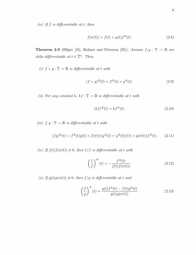
(iv) If f is differentiable at t, then

f(σ(t)) = f(t) + µ(t)f∆(t). (2.8)

Theorem 2.9 (Hilger [45], Bohner and Peterson [28]). Assume f, g : T → R are

delta differentiable at t ∈ Tκ. Then

(i) f + g : T→ R is differentiable at t with

(f + g)∆(t) = f∆(t) + g∆(t). (2.9)

(ii) For any constant k, kf : T→ R is differentiable at t with

(kf)∆(t) = kf∆(t). (2.10)

(iii) f, g : T→ R is differentiable at t with

(fg)∆(t) = f∆(t)g(t) + f(σ(t))g∆(t) = g∆(t)f(t) + g(σ(t))f∆(t). (2.11)

(iv) If f(t)f(σ(t)) 6= 0, then 1/f is differentiable at t with

(1

f

)∆

(t) = − f∆(t)

f(t)f(σ(t)). (2.12)

(v) If g(t)g(σ(t)) 6= 0, then f/g is differentiable at t and

(f

g

)∆

(t) =g(t)f∆(t)− f(t)g∆(t)

g(t)g(σ(t)). (2.13)

9

2.3. INTEGRATION

Definition 2.10. We say f : T → R is right-dense continuous (rd-continuous) pro-

vided f is continuous at each right-dense point t ∈ T and whenever t ∈ T is left-dense,

lims→t−

f(s)

exists as a finite number.

For example, the function µ : T→ R in case T = [0, 1]∪N is rd-continuous but

not continuous at 1. Note that if T = R, then f : R→ R is rd-continuous on T if and

only if f is continuous on T. Also note that if T = Z, then any function f : Z → R

is rd-continuous. We now state some elementary results concerning rd-continuous

functions.

Theorem 2.11. (i) Any continuous function on T is also rd-continuous on T.

(ii) If f is rd-continuous on T, then f σ is rd-continuous on Tκ.

(iii) If f and g are rd-continuous on T, then f + g and fg are rd-continuous on T.

(iv) If f is continuous and g is rd-continuous, then f g is rd-continuous.

Definition 2.12. A function F : T→ R is called a delta antiderivative of f : T→ R

provided F∆(t) = f(t) holds for all t ∈ Tκ. In this case we define the integral of f by

∫ t

a

f(s)∆s = F (t)− F (a)

for all t ∈ T.

Hilger [45] proved that every rd-continuous function on T has a delta an-

tiderivative. Using the different properties of differentiation, one can prove the fol-

lowing properties of the integral.

Theorem 2.13 (Bohner and Peterson [28]). Assume f, g : T→ R are rd-continuous.

Then the following hold.

10

(i)∫ ba[f(t) + g(t)]∆t =

∫ baf(t)∆t+

∫ bag(t)∆t,

(ii)∫ bakf(t)∆t = k

∫ baf(t)∆t,

(iii)∫ baf(t)∆t = −

∫ abf(t)∆t,

(iv)∫ baf(t)∆t =

∫ caf(t)∆t+

∫ bcf(t)∆t,

(v)∫ baf(σ(t))g∆(t)∆t = [f(t)g(t)]ba −

∫ baf∆(t)g(t)∆t,

(vi)∫ baf(t)g∆(t)∆t = [f(t)g(t)]ba −

∫ baf∆(t)g(σ(t))∆t,

(vii)∫ aaf(t)∆t = 0,

where a, b, c ∈ T.

In the following theorem we give a well-known formula that we use frequently

in later sections.

Theorem 2.14. Assume f : T→ R is rd-continuous and t ∈ Tκ. Then

∫ σ(t)

t

f(τ)∆τ = µ(t)f(t). (2.14)

Theorem 2.15 (Hilger [45]). Assume a, b ∈ T and f : T→ R is rd-continuous. Then

the integral has the following properties.

(i) If T = R, then∫ baf(t)∆t =

∫ baf(t)dt, where the integral on the right-hand side

is the Riemann integral.

(ii) If T consists of isolated points, then

∫ b

a

f(t)∆t =

∑t∈[a,b) f(t)µ(t) if a < b

0 if a = b

−∑

t∈[b,a) f(t)µ(t) if a > b.

11

(iii) If T = hZ, where h > 0, then

∫ b

a

f(t)∆t =

∑ bh−1

k= ahf(kh)h if a < b

0 if a = b

−∑ a

h−1

k= bh

f(kh)h if a > b.

(iv) If T = Z, then

∫ b

a

f(t)∆t =

∑b−1t=a f(t) if a < b

0 if a = b

−∑a−1

t=b f(t) if a > b.

(v) If T = qN0, where q > 1, then

∫ b

a

f(t)∆t =

(q − 1)

∑t∈[a,b) tf(t) if a < b

0 if a = b

−(q − 1)∑

t∈[b,a) tf(t) if a > b.

2.4. GENERALIZED POLYNOMIALS

The generalized polynomials gk, hk [1,28] are the functions gk, hk : T×T→ R,

k ∈ N0, defined recursively as follows. The functions g0 and h0 are

g0(t, s) = h0(t, s) ≡ 1 for all s, t ∈ T, (2.15)

and given gk and hk for k ∈ N0, the functions gk+1 and hk+1 are

gk+1(t, s) =

∫ t

s

gk(σ(τ), s)∆τ for all s, t ∈ T (2.16)

12

and

hk+1(t, s) =

∫ t

s

hk(τ, s)∆τ for all s, t ∈ T. (2.17)

If we let h∆k (t, s) denote for each fixed s the derivative of hk(t, s) with respect to t,

then

h∆k (t, s) = hk−1(t, s) for k ∈ N, t ∈ Tκ. (2.18)

Similarly,

g∆k (t, s) = gk−1(σ(t), s) for k ∈ N, t ∈ Tκ. (2.19)

Here are some examples of polynomials in different time scales.

Example 2.16 (Bohner and Peterson [28]). (i) If T = R and k ∈ N0, then

gk(t, s) = hk(t, s) =(t− s)k

k!for all s, t ∈ R.

(ii) If T = Z and k ∈ N0, then

hk(t, s) =

(t− sk

)for all s, t ∈ Z

and

gk(t, s) =

(t− s+ k − 1

k

)for all s, t ∈ Z.

Here(αβ

)is the binomial coefficient defined by

(αβ

)= α(β)

Γ(β+1)for all α, β ∈ C such

that the right-hand side of this equation makes sense, where Γ is the gamma

function and α(β) is the factorial function defined by α(β) := Γ(α+1)Γ(α−β+1)

whenever

the right-hand side is defined.

(iii) If T = qZ and q > 1, then

hk(t, s) =k−1∏i=0

t− qis∑ij=0 q

jfor all s, t ∈ T

13

and

gk(t, s) =k−1∏i=0

qis− t∑ij=0 q

jfor all s, t ∈ T.

2.5. EXPONENTIAL FUNCTIONS

We will start with some technical notions given by Hilger [45] to define the

exponential function on a general measure chain. He studies the complex exponential

function on a measure chain as well. For h > 0, let Zh be

Zh :=z ∈ C : −π

h< Im(z) ≤ π

h

,

and let Ch be defined by

Ch :=

z ∈ C : z 6= −1

h

.

For h = 0, let Z0 = C0 = C, the set of complex numbers.

Definition 2.17. For h > 0, the cylinder transformation ξh is defined by

ξh(z) =1

hLog(1 + zh),

where Log is the principal logarithm function. For h = 0, we define ξ0(z) = z for all

z ∈ Z0 = C.

Definition 2.18. We say that a function p : T→ R is regressive on T provided

1 + µ(t)p(t) 6= 0 for all t ∈ T.

The set of all regressive functions R (Bohner and Peterson [29]) on a time

scale T forms an Abelian group under the addition ⊕ defined by

p⊕ q := p+ q + µpq.

14

The additive inverse in this group is denoted by

p := − p

1 + µp.

We then define subtraction on the set of regressive functions by

p q := p⊕ (q).

It can be shown that

p q =p− q

1 + µq.

Definition 2.19. We define the set R+ of all positively regressive elements of R by

R+ = p ∈ R : 1 + µ(t)p(t) > 0 for all t ∈ T.

Definition 2.20. If p : T → R is regressive and rd-continuous, then we define the

exponential function ep(·, ·) by

ep(t, s) = exp

(∫ t

s

ξµ(τ)(p(τ))∆τ

)

for t ∈ T, s ∈ Tκ, where ξh is the cylinder transformation.

Definition 2.21. The first order linear dynamic equation

y∆ = p(t)y (2.20)

is said to be regressive provided p is regressive and rd-continuous on T.

Theorem 2.22 (Hilger [45]). Assume the dynamic equation (2.20) is regressive and

fix t0 ∈ Tκ. Then ep(·, t0) is the unique solution of the initial value problem

y∆ = p(t)y, y(t0) = 1 (2.21)

on T.

15

Theorem 2.23. Let t0 ∈ T and y0 ∈ R. The unique solution of the initial value

problem

y∆ = p(t)y, y(t0) = y0 (2.22)

is given by

y = ep(·, t0)y0. (2.23)

We next give the variation of constants formulas for first order linear equations.

Theorem 2.24 (Bohner and Peterson [28]). Suppose p ∈ R and f : T → R is rd-

continuous. Let t0 ∈ T and x0 ∈ R. The unique solution of the initial value problem

x∆ = −p(t)xσ + f(t), x(t0) = x0 (2.24)

is given by

x(t) = ep(t, t0)x0 +

∫ t

t0

ep(t, τ)f(τ)∆τ. (2.25)

Theorem 2.25 (Bohner and Peterson [28]). Suppose p ∈ R and f : T → R is rd-

continuous. Let t0 ∈ T and y0 ∈ R. The unique solution of the initial value problem

y∆ = p(t)y + f(t), y(t0) = y0 (2.26)

is given by

y(t) = ep(t, t0)y0 +

∫ t

t0

ep(t, σ(τ))f(τ)∆τ. (2.27)

We next give some important properties of the exponential function.

Theorem 2.26 (Bohner and Peterson [28]). Assume p, q : T→ R are regressive and

rd-continuous. Then the following hold.

(i) e0(t, s) ≡ 1 and ep(t, t) ≡ 1,

(ii) ep(σ(t), s) = (1 + µ(t)p(t))ep(t, s),

(iii) 1/ep(t, s) = ep(s, t) = ep(t, s),

16

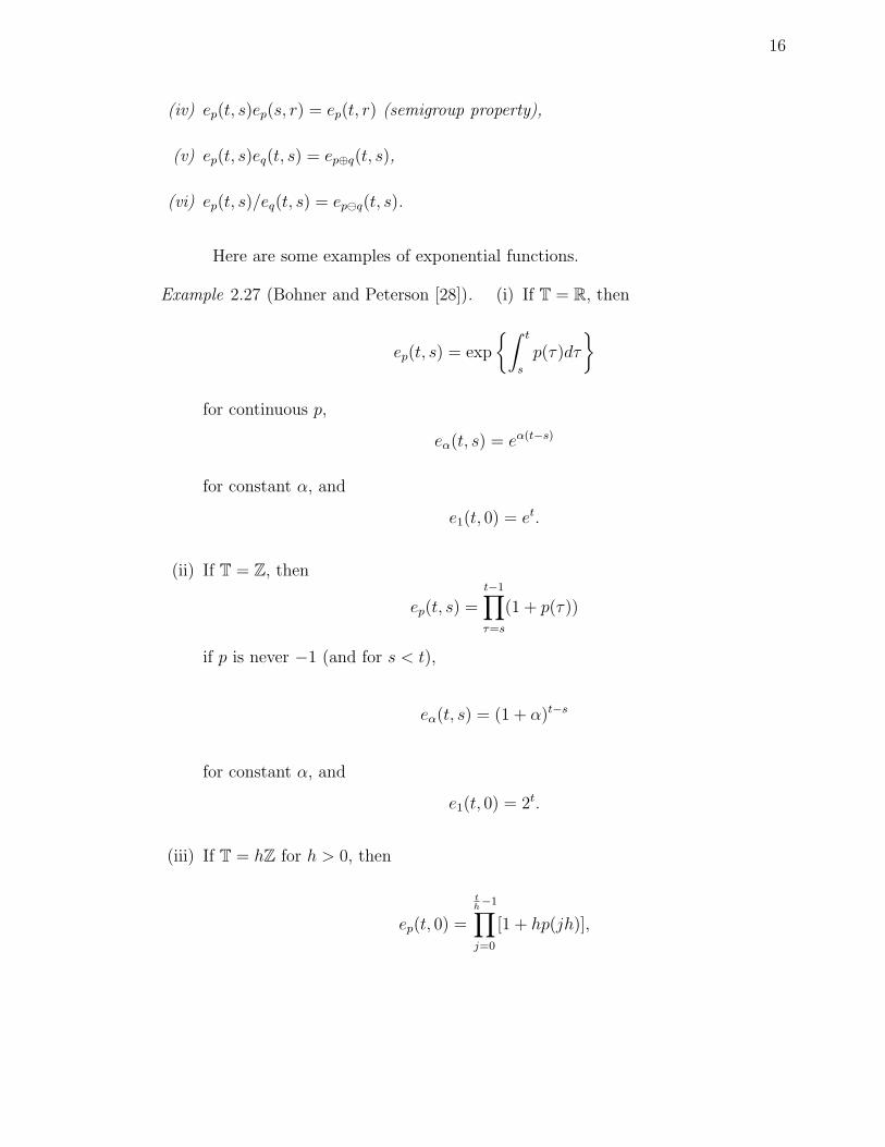
(iv) ep(t, s)ep(s, r) = ep(t, r) (semigroup property),

(v) ep(t, s)eq(t, s) = ep⊕q(t, s),

(vi) ep(t, s)/eq(t, s) = epq(t, s).

Here are some examples of exponential functions.

Example 2.27 (Bohner and Peterson [28]). (i) If T = R, then

ep(t, s) = exp

∫ t

s

p(τ)dτ

for continuous p,

eα(t, s) = eα(t−s)

for constant α, and

e1(t, 0) = et.

(ii) If T = Z, then

ep(t, s) =t−1∏τ=s

(1 + p(τ))

if p is never −1 (and for s < t),

eα(t, s) = (1 + α)t−s


e1(t, 0) = 2t.

(iii) If T = hZ for h > 0, then

ep(t, 0) =

th−1∏j=0

[1 + hp(jh)],

17

for regressive p (and for t > 0),

eα(t, s) = (1 + hα)t−sh


e1(t, 0) = (1 + h)th .

(iv) If T = qN0 = qk : k ∈ N0, where q > 1, then it is easy to show that

ep(t, 1) =√t exp

(− ln2(t)

2 ln(q)

)

if p(t) := (1− t)/((q − 1)t2).

(v) If T = N20 = k2 : k ∈ N0, then

e1(t, 0) = 2√t(√t)!

(vi) If Hn are the harmonic numbers

H0 = 0 and Hn =n∑k=1

1

nfor nN

and

T = Hn : n ∈ N0,

then

eα(Hn, 0) =

(n+ α

n

).

18

3. STOCHASTIC DIFFERENTIAL EQUATION

In this section we give some basic results from stochastic differential equations,

which we attempt to extend to time scales in the subsequent sections.

A stochastic process is a phenomenon which evolves with time in a random

way. Thus, a stochastic process is a family of random variables X(t), indexed by time

(or in a more general framework by a set T ). A realization or sample function of a

stochastic process X(t)t∈T is an assignment, to each t ∈ T , of a possible value of

X(t). So we obtain a random curve which is referred to as a trajectory or a path of

X.

A basic but very important example of a stochastic process is the Brownian

motion process, whose name derives from the observation in 1827 by Robert Brown

of the motion of the pollen particles in a liquid [31].

3.1. PROBABILITY THEORY

In this subsection we state some concepts from general probability theory. We

refer the reader to [43,62,97] for more information.

Definition 3.1. If Ω is a given set, then a σ-algebra on Ω is a family F of subsets of

Ω with the following properties:

(i) ∅ ∈ F ,

(ii) F ∈ F implies FC ∈ F , where FC = Ω\F is the complement of F in Ω,

(iii) A1, A2, . . . ∈ F implies⋃∞i=1 Ai ∈ F .

The pair (Ω,F) is called a measurable space.

Definition 3.2. A probability measure P on a measurable space (Ω,F) is a function

P : F → [0, 1] such that

19

(i) P(∅) = 1, P(Ω) = 1,

(ii) if A1, A2, . . . ∈ F and Ai∞i=1 is disjoint (i.e., Ai ∩ Aj = ∅ if i 6= j), then

P

(∞⋃i=1

Ai

)=∞∑i=1

P(Ai).

The triple (Ω,F ,P) is called a probability space. It is called a complete probability

space if F contains all subsets G of Ω with P-outer measure zero, i.e., with

P∗(G) := infP(G) : F ∈ F , G ⊂ F = 0.

We note that any probability space can be made complete by adding to F all

sets of outer measure 0 and by extending P accordingly. The subsets F of Ω which

belong to F are called F -measurable sets.

Definition 3.3. If (Ω,F ,P) is a given probability space, then a function X : Ω→ R

is called F -measurable if

X−1(U) := ω ∈ Ω : X(ω) ∈ U ∈ F

for all open sets U ⊂ R.

In the following we let (Ω,F ,P) denote a given complete probability space. A

random variable X is an F -measurable function X : Ω→ R. Every random variable

induces a probability measure λX on R, defined by

λX(B) = P(X−1(B)).

λX is called the distribution of X.

Definition 3.4. If∫

Ω|X(ω)|dP(ω) <∞, then the number

E[X] :=

∫Ω

X(ω)dP(ω) =

∫R

xdλX(x)

20

is called the expectation E of X (w.r.t. P).

Definition 3.5. If∫

Ω|X(ω)|2dP(ω) <∞, then the variance of a random variable X

is given by

V[X] = E[(X − E[X])2

]= E

[X2]− (E[X])2.

Definition 3.6. The covariance between two random variables X and Y is given by

Cov [X, Y ] = E [(X − E[X])(Y − E[Y ])] = E[XY ]− E[X]E[Y ].

Definition 3.7. Two subsets A,B ∈ F are called independent if

P(A ∩B) = P(A) · P(B).

A collectionA = Hi : i ∈ I of families ofHi of measurable sets is called independent

if

P(Hi1 ∩Hi2 ∩ · · · ∩Hik) = P(Hi1) · · ·P(Hik)

for all choices ofHi1 ∈ Hi1 , · · · , Hik ∈ Hik with different indices i1, . . . , ik. A collection

of random variables Xi : i ∈ I is called independent if the collection of generated

σ-algebras HXi is independent.

If two random variables X, Y : Ω → R are independent, then E[XY ] =

E[X]E[Y ], provided that E[|X|] <∞ and E[|Y |] <∞.

Next we discuss conditional expectation.

Definition 3.8. Let (Ω,F ,P) be a probability space and let X : Ω→ R be a random

variable such that E [|X|] < ∞. If H ⊂ F is a σ-algebra, then the conditional

expectation of X given H, is defined as E [X|H] =: Y , where Y is a random variable

satisfying

(i) E [|Y |] <∞,

(ii) E [X|H] is H-measurable,

21

(iii)∫H

E [X|H] dP =∫HXdP for all H ∈ H.

We list some of the basic properties of the conditional expectation.

Theorem 3.9. Suppose Y : Ω→ R is another random variable with E [Y ] <∞ and

let a, b ∈ R. Then

(i) E [aX + bY |H] = aE [X|H] + bE [Y |H],

(ii) E [E [X|H]] = E [X],

(iii) E [X|H] = X if X is H-measurable,

(iv) E [X|H] = E [X] if X is independent of H,

(v) E [Y X|H] = Y E [X|H] if Y is H-measurable.

Next we define filtration and martingales.

Definition 3.10. A filtration on (Ω,F) is a family M = M(t)t∈T of σ-algebras

M(t) ⊂ F such that

t0 ≤ s < t implies M(s) ⊂M(t),

i.e., M(t) is increasing.

Definition 3.11. A stochastic process M(t)t∈T on (Ω,F ,P) is called a martingale

with respect to a filtration M(t)t∈T and with respect to P if

(i) M(t) is M(t)-measurable for all t ∈ T

(ii) E[|M(t)|] <∞ for all t ∈ T and

(iii) E[M(s)|M(t)] = M(t) for all s, t ∈ T with s ≥ t.

22

If (iii) above is replaced by

E[M(s)|M(t)] ≤M(t) for all s, t ∈ T with s ≥ t

then M(t)t∈T is called a supermartingale and if (iii) above is replaced by

E[M(s)|M(t)] ≥M(t) for all s, t ∈ T with s ≥ t

then M(t)t∈T is called a submartingale.

3.2. STOCHASTIC DIFFERENTIAL EQUATIONS

In this subsection we give a brief introduction to stochastic differential equa-

tions. Let us fix x0 ∈ R and for t > 0 consider the ordinary differential equation

dx

dt= a(x(t)), x(0) = x0, (3.1)

where a : R→ R is given and the solution is the trajectory x : [0,∞)→ R.

In many applications, the experimentally measured trajectories of systems

modeled by (3.1) do not behave as predicted. Hence, it is reasonable to modify (3.1),

somehow to include the possibility of random effects disturbing the system. A formal

way to do so is to write

dX

dt= a(X(t)) + b(X(t))ζ(t), X(0) = X0 (3.2)

where b : R→ R and ζ is white noise.

This approach presents us with these mathematical problems:

• Define what it means for X to solve (3.2).

• Show (3.2) has a solution, discuss asymptotic behavior, dependence upon X0,

a, b, etc.

23

If we let X0 = 0, a ≡ 0, and b ≡ 1, then the solution of (3.2) turns out to be the

Wiener process or Brownian motion denoted by W . Thus, we may symbolically write

dW/dt = ζ, thereby asserting that white noise is the time derivative of the Wiener

process. Returning to (3.2), we have

dX

dt= a(X(t)) + b(X(t))

dW

dt,

which gives us

dX = a(X(t))dt+ b(X(t))dW, X(0) = X0. (3.3)

This expression is a stochastic differential equation. We say that X solves (3.3)

provided

X(t) = X0 +

∫ t

0

a(X(s)) ds+

∫ t

0

b(X(s)) dW (3.4)

for all t > 0. Now we must

• Construct W .

• Define the stochastic integral.

• Find explicit solutions in special cases.

Next we look at the chain rule in stochastic calculus.

Definition 3.12. We denote by Lp(0, T ), for p ≥ 1, the space of all real-valued,

progressively measurable stochastic processes X such that

E[∫ T

0

|X|p(t) dt]<∞. (3.5)

Theorem 3.13 (Ito’s Lemma). Suppose that X has a stochastic differential

dX = F (t)dt+G(t)dW,

for F ∈ L1(0, T ), G ∈ L2(0, T ). Assume u : R × [0, T ] → R is continuous and that

∂u/∂t, ∂u/∂x, ∂2u/∂x2 exist and are continuous. Set Y (t) := u(X(t), t). Then Y

24

has the stochastic differential

dY =∂u(X(t), t)

∂tdt+

∂u(X(t), t)

∂xdX +

1

2

∂2u(X(t), t)

∂x2G2dt

=

(∂u(X(t), t)

∂t+∂u(X(t), t)

∂xF (t) +

1

2

∂2u(X(t), t)

∂x2G2(t)

)dt

+∂u(X(t), t)

∂xG(t) dW. (3.6)

Example 3.14. Let us suppose that g is a continuous function. Then the unique

solution of

dY = g(t)Y dW, Y (0) = 1 (3.7)

is

Y (t) = exp

(−1

2

∫ t

0

g2(s) ds+

∫ t

0

g(s) dW

)(3.8)

for 0 ≤ t ≤ T . To verify this, note that

X(t) := −1

2

∫ t

0

g2(s) ds+

∫ t

0

g(s) dW

satisfies

dX = −1

2g2(t) dt+ g(t) dW.

Thus, Ito’s lemma for u(x) = ex gives

dY =∂u (X(t))

∂xdX +

1

2

∂2u (X(t))

∂x2g2(t) dt

= eX(t)

(−1

2g2(t) dt+ g(t) dW +

1

2g2(t) dt

)= g(t)Y dW,

as claimed.

Example 3.15. Similarly, the unique solution of

dY = f(t)Y dt+ g(t)Y dW, Y (0) = 1 (3.9)

25

is

Y (t) = exp

(∫ t

0

(f − 1

2g2

)(s) ds+

∫ t

0

g(s) dW

)(3.10)

for 0 ≤ t ≤ T .

Example 3.16. Let S(t) denote the price of a stock at time t. We can model the

evolution of S(t) in time by supposing that dSS

, the relative change of price, evolves

according to the SDEdS

S= αdt+ βdW

for certain constants α > 0 and β, called the drift and volatility of the stock. Hence,

dS = αSdt+ βSdW, (3.11)

and so by Ito’s formula

d(log(S)) =dS

S− 1

2

β2S2dt

S2

=

(α− β2

2

)dt+ βdW.

Consequently

S(t) = S0 exp

(βW (t) +

(α− β2

2

)t

).

The mean of S(t) is given by

E [S(t)] = S0 exp (α(t− t0)) (3.12)

and its variance is

V [S(t)] = S20 exp (2α(t− t0))

[exp

(β2(t− t0)

)− 1]. (3.13)

We refer to [56,93] for further applications of stochastic differential equations.

For a short history of stochastic integration and mathematical finance we refer to [53],

and for Stratonovic stochastic integrals we refer to [88–90].

26

4. CONSTRUCTION OF BROWNIAN MOTION

In this section we construct Brownian motion on an isolated time scale. We

also present some of the basic properties of Brownian motion.

4.1. BROWNIAN MOTION

4.1.1. Historical Remarks and Basic Definitions. In 1828, Robert

Brown published a brief account of the microscopical observations made in the months

of June, July and August, 1827 on the particles contained in the pollen of plants [31].

In 1900, Bachelier [14] postulated that stock prices execute Brownian motion, and he

developed a mathematical theory which was similar to the theory which Einstein [36]

developed. In 1923, Norbert Wiener proved the existence of Brownian motion and

made significant contributions to related mathematical theories, so Brownian motion

is often called a Wiener process [96].

This new branch of mathematics blossomed from the pioneering work of Kiyosi

Ito [49–52]. Probably his most influential contribution was the development of an

equation that describes the evolution of a random variable driven by Brownian mo-

tion. Ito’s lemma, as mathematicians now call it, is a series expansion of a stochastic

function giving the total differential.

The mathematical theory of Brownian motion has been applied in contexts

ranging far beyond the movement of particles in fluids. In 1973, Fischer Black, My-

ron Scholes and Robert Merton [18, 60] used stochastic analysis and an equilibrium

argument to compute a theoretical value for an options’ price. This is now called the

Black and Scholes option price formula or Black and Scholes model.

This brief list, of course, does not do justice to the work of many other people

who have written about Brownian motion.

27

4.1.2. Stochastic Processes. We begin our study by defining a stochastic

process on a time scale.

Definition 4.1. A stochastic process is a parameterized collection of random vari-

ables

X(t)t∈T

defined on a probability space (Ω,F ,P) and assuming values in R.

The parameter space T is usually the half line [0,∞), but it may also be an

interval [a, b], the nonnegative integers and even subsets of R. In this dissertation,

we focus on those parameter spaces for which ρ(t) < t < σ(t) for all t ∈ T. Such a

parameter space is called an isolated time scale (Definition 2.4). We will denote an

isolated time scale by T throughout.

An important class of stochastic processes are those with independent incre-

ments, that is, for which the random variables ∆X(t)t∈T are independent for any

finite combination of time instants in T. A Brownian motion or a standard Wiener

process W = W (t)t∈T is an example of a stochastic process with independent in-

crements which we define next.

Definition 4.2. A real-valued stochastic process W is called a Brownian motion or

Wiener process on T if

(i) W (t0) = 0 a.s.,

(ii) W (t)−W (s) ∼ N (0, t− s) for all t0 ≤ s ≤ t ∈ T ,

(iii) for all times ti0 < ti1 < ti2 < . . . < tin , the random variables

W (ti0),W (ti1)−W (ti0), . . . ,W (tin)−W (tin−1)

are independent (independent increments),

for t0, t, s ∈ T and N (0, t − s) is the normal distribution with mean 0 and variance

t− s.

28

Theorem 4.3. For an isolated time scale T = t0, t1, t2, . . ., W is Brownian motion

if and only if

(i) W (t0) = 0 a.s.,

(ii) ∆W (t) ∼ N (0, µ(t)) for all t ∈ T,

(iii) for all t ∈ T, the random variables ∆W (t) are independent ( independent incre-

ments).

Proof. It is obvious that Definition 4.2 reduces to the assumptions of this theorem if

we choose tji = tj for j ∈ N0. To see that Definition 4.2 follows from the assumption

of this theorem we observe that for t0 < tm < tn,∑n−1

i=mN (0, µ(ti)) has the same

distribution as N(0,∑n−1

i=m µ(ti))

or N (0, tn − tm).

4.1.3. Properties of Brownian Motion. In this part, we prove some of

the basic properties of Brownian motion which we use in subsequent sections.

Lemma 4.4. E[W (t)] = 0 and E[W 2(t)] = t− t0 for each time t ≥ t0.

Proof. We observe that W (t)−W (t0) ∼ N (0, t− t0) and that

E[W (t)−W (t0)] = E[W (t)] = 0

and

E[W 2(t)] = E[W 2(t)]− (E[W (t)])2

= V[W (t)]

= V[W (t)−W (t0)]

= t− t0.

This concludes the proof.

29

Definition 4.5. For t, s ∈ T, we define t ∧ s as the minimum of t and s.

Lemma 4.6. Suppose W is a one-dimensional Brownian motion. Then

E[W (t)W (s)] = (t ∧ s)− t0 for all t, s ∈ T. (4.1)

Proof. Let us assume t0 ≤ s < t. Then

Cov[W (t),W (s)] = E[W (t)W (s)] = E[(W (s) +W (t)−W (s))W (s)]

= E[W 2(s)] + E[(W (t)−W (s))W (s)]

= s− t0 + E[W (t)−W (s)] E[W (s)]︸︷︷︸=0

= s− t0

= (t ∧ s)− t0,

since W (s) ∼ N (0, s) and W (t)−W (s) is independent of W (s).

Theorem 4.7. Brownian motion W (t)t∈T is a martingale w.r.t. the σ-algebras F(t)

generated by W (s) : s ≤ t.

Proof. We show that W satisfies the conditions given in Definition 3.11. From

Cauchy–Schwarz inequality we have,

(E[W (t)])2 ≤ E[|W (t)|2] = t− t0.

Also, for all t0 ≤ s ≤ t <∞ and t0, s, t ∈ T, we have

E [W (t)|F(s)] = E [W (s) +W (t)−W (s)|F(s)]

= E [W (s)|F(s)] + E [(W (t)−W (s))|F(s)]

= W (s) + 0 = W (s).

Here we have used that E [W (t)−W (s)|F(s)] = 0 since W (t)−W (s) is independent

30

of F(t) and we have used that E [W (s)|F(s)] = W (s) since W (s) is F(s)-measurable.

Theorem 4.8. W 2(t)− t is a martingale.

Proof. For t > s > t0 we have

E[W 2(t)− t|F(s)

]= E

[W 2(t)|F(s)

]− t

= E[(W (s) +W (t)−W (s))2|F(s)

]− t

= E[W 2(s)|F(s)

]− 2E [W (s)(W (t)−W (s))|F(s)]

+ E[(W (t)−W (s))2|F(s)

]− t

= W 2(s) + 2W (s)E [W (t)−W (s)|F(s)]

+ E[(W (t)−W (s))2|F(s)

]− t

= W 2(s) + 0 + t− s− t

= W 2(s)− s,

where on the fourth equality we have used Definition 4.2.

Theorem 4.9. Suppose c > 0. Let Wc be a Brownian motion on Tc := c2t : t ∈ T

with Wc(c2t0) = 0. Then W (t) := c−1Wc(c

2t) is a Brownian motion on T.

Proof. We have E [W (t)] = c−1E [Wc(c2t)] = 0 and V [W (t)] = c−2c2t = t. Also

Cov [W (t),W (s)] = c−1c−1Cov[Wc(c

2t),Wc(c2s)]

= c−2[(c2t ∧ c2s)− c2t0

]= (t ∧ s)− t0,

where in the second equality we have used Lemma 4.6.

Next we give some possible directions about constructing a Wiener process on

isolated time scales.

31

4.2. BUILDING A ONE-DIMENSIONAL BROWNIAN MOTION

The existence of the Brownian motion process follows from Kolmogorov’s ex-

istence theorem [17]. Our method will be to develop a formal expansion of ∆W

in terms of an orthonormal basis of L2∆(T) functions on T. We then integrate the

resulting expression in time and prove then that we have built a Wiener process.

Theorem 4.10 (Agarwal, Otero-Espinar, Perera, Vivero [2]). Let Jo = [t0, t) ∩ T,

t0, t ∈ T, t0 < t, be an arbitrary closed interval of T. Then, the set Lp∆(Jo) is a

Banach space together with the norm defined for every f ∈ Lp∆(Jo) as

||f ||Lp∆ :=

[∫Jo|f |p(τ)∆τ

]1/p

for p ∈ R. (4.2)

Moreover, L2∆(Jo) is a Hilbert space together with the inner product given for every

(f, g) ∈ L2∆(Jo)× L2

∆(Jo) by

(f, g)L2∆

:=

∫Jof(τ)g(τ)∆τ. (4.3)

Definition 4.11. Two functions f, g : T→ R are orthonormal over Jo = [t0, t)∩T if

(i) (f, g)L2∆

=∫Jof(τ)g(τ)∆τ = 0, and

(ii) ||f ||L2∆

= ||g||L2∆

=[∫Jo|f |2(τ)∆τ

]1/2=[∫Jo|g|2(τ)∆τ

]1/2= 1.

4.2.1. Haar Functions. The Haar function is the first known wavelet and

was proposed in 1909 by Alfred Haar [41]. We use Haar functions on isolated time

scales to construct Brownian motion.

Definition 4.12. The family hmnm,n∈N0 of Haar functions is defined for t ∈ T as

follows:

h00(t) =1√∑

ti∈T µ(ti)for t ∈ T.

32

For n ∈ N, we let n′ = n− 1. Then

h0n(t) =

√µ(t2n′+1)

µ(t2n′ )[µ(t2n′ )+µ(t2n′+1)]if t = t2n′

−√

µ(t2n′ )µ(t2n′+1)[µ(t2n′ )+µ(t2n′+1)]

if t = t2n′+1

0 otherwise,

h1n(t) =

√µ(t4n′+2)+µ(t4n′+3)

[µ(t4n′ )+µ(t4n′+1)][µ(t4n′ )+µ(t4n′+1)+µ(t4n′+2)+µ(t4n′+3)]if t = t4n′ , t4n′+1

−√

µ(t4n′ )+µ(t4n′+1)

[µ(t4n′+2)+µ(t4n′+3)][µ(t4n′ )+µ(t4n′+1)+µ(t4n′+2)+µ(t4n′+3)]if t = t4n′+2, t4n′+3

0 otherwise.

In general for m ∈ N0, n ∈ N and n′ = n− 1, we have

hmn(t) =

√ ∑2k−1i=k µ(ti+2n′k)∑k−1

i=0 µ(ti+2n′k)∑2k−1i=0 µ(ti+2n′k)

if t2n′k ≤ t ≤ t2n′k+k−1

−√ ∑k−1

i=0 µ(ti+2n′k)∑2k−1i=k µ(ti+2n′k)

∑2k−1i=0 µ(ti+2n′k)

if t2n′k+k ≤ t ≤ t2n′k−2k−1

0 otherwise,

where k = 2m.

Example 4.13. When T = Z we have µ(t) = 1. In this case the Haar functions are

33

given by

h0n(t) =

√12

if t = t2n

−√

12

if t = t2n−1

0 otherwise,

h1n(t) =

√14

if t = t4n, t4n+1

−√

14

if t = t4n+2, t4n+3

0 otherwise.

In general, we have

hmn(t) =

√1

2m+1 if tn2m+1 ≤ t ≤ tn2m+1+2m−1

−√

12m+1 if tn2m+1+2m ≤ t ≤ tn2m+1+2m+1−1

0 otherwise.

Lemma 4.14. The functions hmnm,n∈N0 form an orthonormal basis of L2∆(T).

Proof. We have

∫Th2mn(t)∆t =

2m−1∑i=0

µ(ti+n2m+1)

[ ∑2m+1−1i=2m µ(ti+n2m+1)∑2m−1

i=0 µ(ti+n2m+1)∑2m+1−1

i=0 µ(ti+n2m+1)

]

+2m+1−1∑i=2m

µ(ti+n2m+1)

[ ∑2m−1i=0 µ(ti+n2m+1)∑2m+1−1

i=2m µ(ti+n2m+1)∑2m+1−1

i=0 µ(ti+n2m+1)

]= 1.

34

Also for m′ > m, either hmnhm′n = 0 for all t or else hmn is constant on the support

of hm′n. In this second case,

∫Thmn(t)hm′n(t)∆t = hmn

∫Thm′n(t)∆t = 0.

This completes the proof.

Example 4.15. For Haar functions in T = qN0 , q > 1, we refer to Table 4.1. To make

the table compact, we let p = q − 1 and [n] =∑n−1

k=0 qk.

Table 4.1: Haar Functions for T = 1, q, q2, q3, q4, q5, q6, q7.

h00(t) h20(t) h10(t) h11(t) h01(t) h02(t) h03(t) h04(t)

1 1√[8]p

q2√[8]p

q√[4]p

0√

q[2]p

0 0 0

q 1√[8]p

q2√[8]p

q√[4]p

0 −1√[2]pq

0 0 0

q2 1√[8]p

q2√[8]p

−1

q√

[4]p0 0 1√

[2]pq0 0

q3 1√[8]p

q2√[8]p

−1

q√

[4]p0 0 −1√

[2]pq30 0

q4 1√[8]p

−1

q2√

[8]p0 1

q√

[4]p0 0 −1√

[2]pq30

q5 1√[8]p

−1

q2√

[8]p0 1

q√

[4]p0 0 −1√

[2]pq50

q6 1√[8]p

−1

q2√

[8]p0 −1

q3√

[4]p0 0 0 1√

[2]pq5

q7 1√[8]p

−1

q2√

[8]p0 −1

q3√

[4]p0 0 0 −1√

[2]pq7

4.2.2. Schauder Functions and Wiener Processes.

Definition 4.16. For m,n ∈ N0,

smn(t) :=

∫ t

t0

hmn(τ)∆τ (4.4)

35

is called the mnth Schauder function.

Let us assume that k = 2m. Then the graph of smn is an open tent lying

above the interval [t2nk, t2nk+2k]. The highest point on this tent can be found in the

following manner.

maxt∈T|smn(t)| =

∫ t2nk+k

t0

hmn(τ)∆τ

=

∫ t2nk+k

t2nk

hmn(τ)∆τ

=k−1∑i=0

µ(ti+2nk)

√ ∑2k−1i=k µ(ti+2nk)∑k−1

i=0 µ(ti+2nk)∑2k−1

i=0 µ(ti+2nk)

=

√∑k−1i=0 µ(ti+2nk)

∑2k−1i=k µ(ti+2nk)∑2k−1

i=0 µ(ti+2nk).

Next we define

W (t) :=∞∑m=0

∞∑n=0

Zmn(ω)smn(t)

for times t ∈ T, where the coefficients Zmnm,n∈N0 are independent and N (0, 1)

random variables defined on some probability space. This series does not converge

for all T. For those for which this series does converge, the following holds.

Lemma 4.17. We have

∞∑m=0

∞∑n=0

smn(t)smn(s) = (t ∧ s)− t0

for each t, s ∈ T.

Proof. For each s ∈ T, let us define

φs(τ) =

1 if t0 ≤ τ ≤ s

0 otherwise.

36

Then using Definition 4.16 and Lemma 4.14, we have

∞∑m=0

∞∑n=0

smn(t)smn(s) =∞∑m=0

∞∑n=0

∫ t

t0

hmn(τ)∆τ

∫ s

t0

hmn(τ)∆τ

=∞∑m=0

∞∑n=0

∫ ∞t0

φt(τ)hmn(τ)∆τ

∫ ∞t0

φs(τ)hmn(τ)∆τ

=

∫ ∞t0

∫ ∞t0

φt(τ)φs(τ)

[∞∑m=0

∞∑n=0

hmn(τ)hmn(τ)

]∆τ∆τ

=

∫ ∞t0

φt(τ)φs(τ)∆τ

=

∫ t∧s

t0

∆τ

= (t ∧ s)− t0,

where we observe that for fixed m,n ∈ N, the above sums and integrals are finite

thereby permitting us to interchange the integrations with summations.

Theorem 4.18. Let Zmnm,n∈N0 be a sequence of independent and N (0, 1) random

variables defined on the same probability space. Then the sum

W (t, ω) :=∞∑m=0

∞∑n=0

Zmn(ω)smn(t),

is a Brownian motion for t ∈ T.

Proof. To prove W is a Brownian motion, we first note that clearly W (t0) = 0 a.s.

We assert that W (t)−W (s) ∼ N (0, t− s) for all s, t ∈ T such that s ≤ t. To prove

this let us compute

E [exp (iλ(W (t)−W (s)))]

= E

[exp

(iλ

∞∑m=0

∞∑n=0

Zmn(smn(t)− smn(s))

)]

=∞∏m=0

∞∏n=0

E [exp (iλZmn(smn(t)− smn(s)))]

37

=∞∏m=0

∞∏n=0

exp

(−λ

2

2(smn(t)− smn(s))2

)

= exp

(−λ

2

2

∞∑m=0

∞∑n=0

(s2mn(t)− 2smn(t)smn(s) + s2

mn(s))

)

= exp

(−λ

2

2(t− t0 − 2(s− t0) + s− t0)

)= exp

(−λ

2

2(t− s)

),

where second equality follows from independence and for the third equality we have

used the fact that Zmn is N (0, 1). By the uniqueness of characteristic functions, the

increment W (t)−W (s) is N (0, t− s) distributed, as asserted. Next we claim for all

p ∈ N and for all t0 < t1 < t2 < . . . < tp, that

E

[exp

(i

p∑j=1

λj(W (tj)−W (tj−1))

)]=

p∏j=1

exp

(−λ2j

2(tj − tj−1)

). (4.5)

Once this is proved, we will know from uniqueness of characteristic functions that

FW (t1),...,W (tp)−W (tp−1)(x1, . . . , xp) = FW (t1)(x1) · · ·FW (tp)−W (tp−1)(xp)

for all x1, x2, . . . , xp ∈ R. This proves that

W (t1), . . . ,W (tp)−W (tp−1) are independent.

Thus, (4.5) will establish the theorem. Now in the case p = 2, we have

E [exp (i[λ1W (t1) + λ2(W (t2)−W (t1))])]

= E [exp (i[(λ1 − λ2)W (t1) + λ2W (t2)])]

= E

[exp

(i(λ1 − λ2)

∞∑m=0

∞∑n=0

Zmnsmn(t1) + iλ2

∞∑m=0

∞∑n=0

Zmnsmn(t2)

)]

=∞∏m=0

∞∏n=0

E [exp (iZmn ((λ1 − λ2)smn(t1) + λ2smn(t2)))]

38

=∞∏m=0

∞∏n=0

exp

(−1

2[(λ1 − λ2)smn(t1) + λ2smn(t2)]2

)

= exp

(−1

2

∞∑m=0

∞∑m=0

[(λ1 − λ2)2s2

mn(t1) + 2(λ1 − λ2)λ2smn(t1)smn(t2)])

+ exp

(−1

2

∞∑m=0

∞∑m=0

λ22s

2mn(t2)

)

= exp

(−1

2

[(λ1 − λ2)2(t1 − t0) + 2(λ1 − λ2)λ2(t1 − t0) + λ2

2(t2 − t0)])

= exp

(−1

2

[λ2

1(t1 − t0) + λ22(t2 − t1)

]), (4.6)

where on the sixth equality we have used Lemma 4.17. We observe that (4.6) is same

as (4.5) for p = 2. The general case follows similarly.

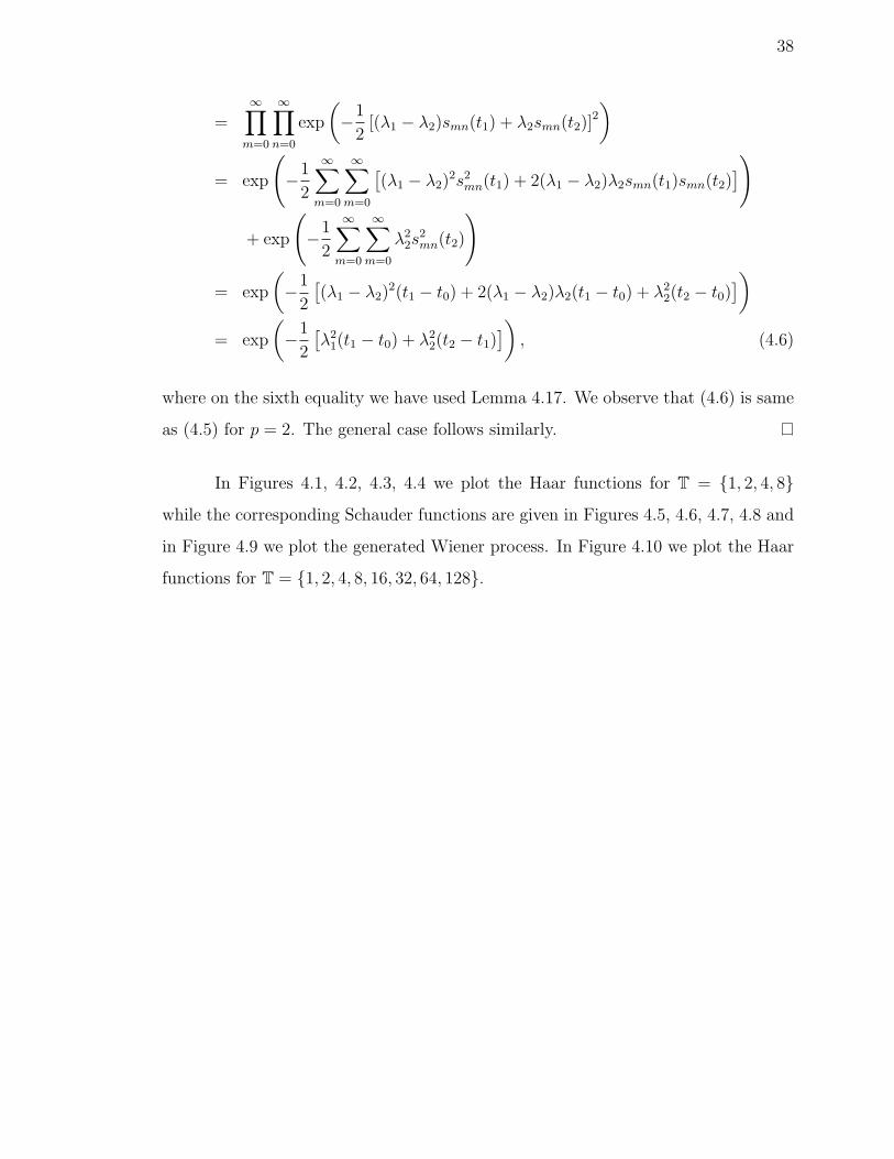
In Figures 4.1, 4.2, 4.3, 4.4 we plot the Haar functions for T = 1, 2, 4, 8

while the corresponding Schauder functions are given in Figures 4.5, 4.6, 4.7, 4.8 and

in Figure 4.9 we plot the generated Wiener process. In Figure 4.10 we plot the Haar

functions for T = 1, 2, 4, 8, 16, 32, 64, 128.

39

-0.4

-0.2

0

0.2

0.4

0.6

0.8

1 2 4 8

h_0

0(t)

t

Haar Function h_00(t) for T=1,2,4,8

'h_00.dat'

Figure 4.1: Haar Function h00(t) for T = 1, 2, 4, 8.

-0.4

-0.2

0

0.2

0.4

0.6

0.8

1 2 4 8

h_0

1(t)

t


'h_01.dat'


40

-0.4

-0.2

0

0.2

0.4

0.6

0.8

1 2 4 8

h_0

2(t)

t


'h_02.dat'


-0.4

-0.2

0

0.2

0.4

0.6

0.8

1 2 4 8

h_1

0(t)

t


'h_10.dat'


41

-1

-0.5

0

0.5

1

1.5

2

2.5

3

1 2 4 8

s_0

0(t)

t

Schauder Function s_00(t) for T=1,2,4,8

's_00.dat'

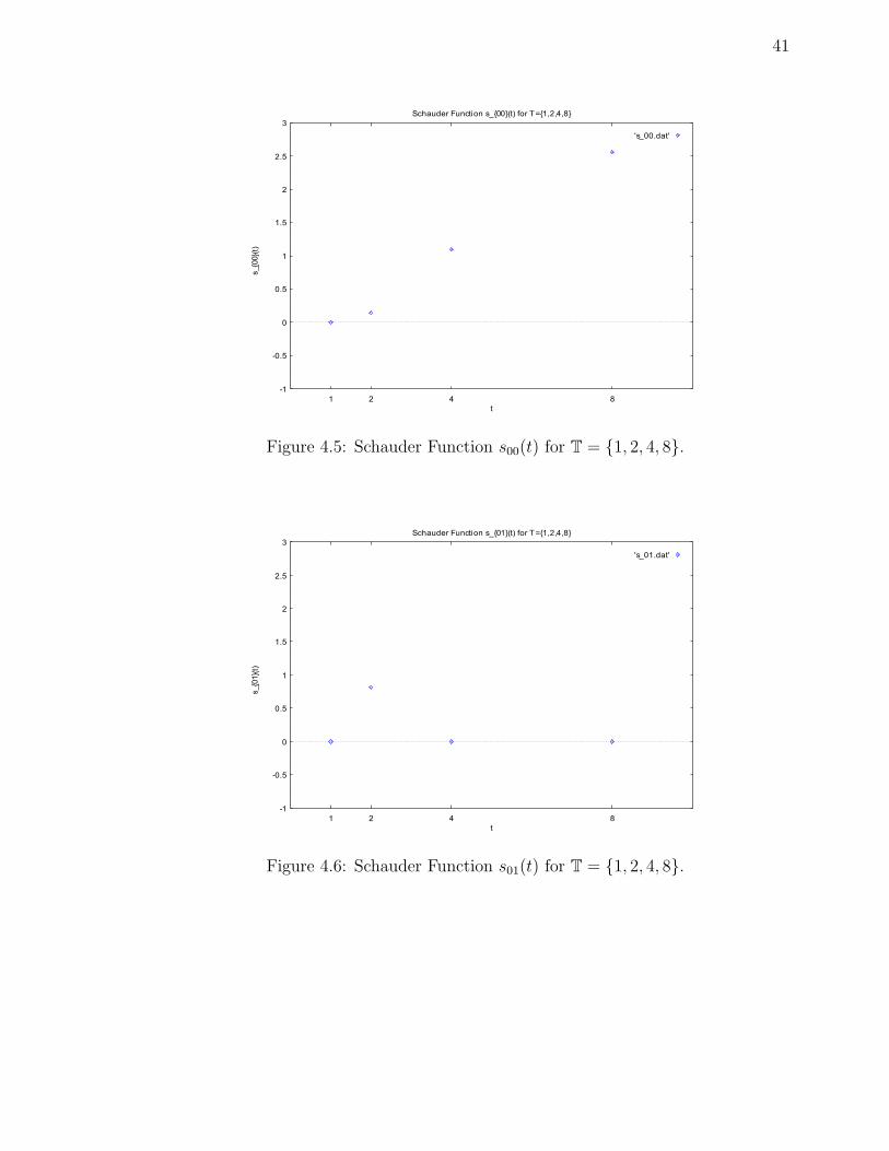
Figure 4.5: Schauder Function s00(t) for T = 1, 2, 4, 8.

-1

-0.5

0

0.5

1

1.5

2

2.5

3

1 2 4 8

s_0

1(t)

t


's_01.dat'


42

-1

-0.5

0

0.5

1

1.5

2

2.5

3

1 2 4 8

s_0

2(t)

t


's_02.dat'


-1

-0.5

0

0.5

1

1.5

2

2.5

3

1 2 4 8

s_1

0(t)

t


's_10.dat'


43

-2

-1.5

-1

-0.5

0

0.5

1

1.5

2

1 2 4 8

W(t)

t

Brownian Motion W(t) for T=1,2,4,8

'brown.dat'

Figure 4.9: Generated Brownian Motion W (t) for T = 1, 2, 4, 8.

-0.1

-0.05

0

0.05

0.1

0.15

0.2

0.25

0.3

12 4 8 16 32 64 128

h_2

0(t)

t

Haar Function h_20(t) for T=1,2,4,8,16,32,64,128

'h_20.dat'

Figure 4.10: Generated Haar Function h20(t) for T = 1, 2, 4, 8, 16, 32, 64, 128.

44

5. STOCHASTIC INTEGRALS

This section provides an introduction to stochastic calculus, in particular to

stochastic integration.

5.1. INTRODUCTION

The stochastic calculus of Ito originated with his investigation of conditions

under which the local properties (drift and the diffusion coefficient) of a Markov

process could be used to characterize this process. This has been used earlier by

Kolmogorov to derive the partial differential equations for the transition probabilities

of a diffusion process. Kiyosi Ito’s [49–52] approach focussed on the functional form

of the processes themselves and resulted in a mathematically meaningful formulation

of stochastic differential equations. A similar theory was developed independently at

about the same time by Gikhman [38–40].

5.2. CONSTRUCTION OF ITO INTEGRAL

An ordinary dynamic equation

x∆ = a(t, x) (5.1)

may be thought of as a degenerate form of a stochastic dynamic equation in the

absence of randomness. We could write (5.1) in the symbolic ∆-differential form

∆x = a(t, x)∆t, (5.2)

or more accurately a ∆-integral equation

x(t) = x0 +

∫ t

t0

a(τ, x(τ))∆τ, (5.3)

45

where x is a solution satisfying the initial condition x(t0) = x0. Stochastic equations

can be written in the form

∆X(t) = a(t,X(t))∆t+ b(t,X(t))ξ(t)∆t, (5.4)

where the deterministic or average drift term (5.1) is perturbed by a noisy term

b(t,X(t))ξ(t), ξ(t) are standard Gaussian random variables for each t, and b(t,X(t))ξ(t)

is a space-time dependent intensity factor. Equation (5.4) is then interpreted as

X(t) = X(t0) +

∫ t

t0

a(τ,X(τ))∆τ +

∫ t

t0

b(τ,X(τ))ξ(τ)∆τ (5.5)

for each sample path. For the special case of (5.5) with a ≡ 0 and b ≡ 1, we see that

ξ(t) should be the ∆ of a Wiener process W , thus suggesting that we could write

(5.5) alternatively as

X(t) = X(t0) +

∫ t

t0

a(τ,X(τ))∆τ +

∫ t

t0

b(τ,X(τ))∆W (τ). (5.6)

For constant b(t, x) ≡ b, we would expect the second integral in (5.6) to be b(W (t)−

W (t0)). To fix ideas, we shall consider such an integral of a random function X over

T, denoting it by I(X), where

I(X) =

∫ t

t0

X(τ)∆W (τ). (5.7)

For a nonrandom step function X(t) = Xt for t ∈ T, we take

I(X) =∑

τ∈[t0,t)

Xτ∆W (τ) a.s. (5.8)

This is a random variable with zero mean since it is the sum of random variables

with zero mean. Let F(t)t∈T be an increasing family of σ-algebras such that W (t)

46

is F(t)-measurable for each t ≥ t0. We consider a random step function

X(t) = Xt

for t ∈ T such that Xt is F(t)-measurable. We also assume that each Xt is mean-

square integrable over Ω. Hence,

E[X2t

]<∞

for t ∈ T. Since

E [∆W (τ)|F(τ)] = 0 a.s.,

it follows that the product Xτ∆W (τ) is F(σ(τ))-measurable, integrable, and

E [Xτ∆W (τ)] = E [Xτ∆W (τ)|F(τ)] = 0

for each τ ∈ T. Analogously to (5.8), we define the integral I(X) by

I(X) =∑

τ∈[t0,t)

Xτ∆W (τ) a.s. (5.9)

Since the Xτ is F(σ(τ))-measurable and hence F(t)-measurable, it follows that I(X)

is F(t)-measurable. In addition, I(X) is integrable over Ω, has zero mean. It is also

mean-square integrable with

E[(I(X))2

]= E

∑τ∈[t0,t)

Xτ∆W (τ)

2∣∣∣∣∣∣F(τ)

=

∑τ∈[t0,t)

E[X2τ

]E[(∆W (τ))2

∣∣F(τ)]

=∑

τ∈[t0,t)

E[X2τ

](σ(τ)− τ)

=∑

τ∈[t0,t)

E[X2τ

]µ (τ) (5.10)

47

on account of the mean-square property of the increments W (σ(τ))−W (τ) for τ ∈ T.

Finally, from (5.9) we have

I (αX + βY ) = αI(X) + βI(Y ) (5.11)

a.s. for α, β ∈ R and any random step functions X, Y satisfying the above properties,

that is, the integration operator I is linear in the integrand.

5.3. QUADRATIC VARIATION

Definition 5.1. If (W (t))t∈T is a Brownian motion defined on some probability space

(Ω,F ,P), then the quadratic variation 〈W,W 〉t is defined by

〈W,W 〉t :=∑

τ∈[t0,t)

(∆W (τ))2, (5.12)

for t ∈ T.

Lemma 5.2. For a Brownian motion W , we have

〈W,W 〉t = W 2(t)−W 2(t0)− 2∑

τ∈[t0,t)

W (τ)∆W (τ) (5.13)

and 〈W,W 〉t = χ(t), where χ(t) is a random variable with

E [χ(t)] =∑

τ∈[t0,t)

µ(τ) =

∫ t

t0

∆τ (5.14)

and

V [χ(t)] = 2∑

τ∈[t0,t)

µ2(τ) = 2

∫ t

t0

µ(τ)∆τ. (5.15)

Proof. We use Definition 5.1 to find

〈W,W 〉t =∑

τ∈[t0,t)

(∆W (τ))2

48

=∑

τ∈[t0,t)

(W 2(σ(τ)) +W 2(τ))−∑

τ∈[t0,t)

2W (σ(τ))W (τ)

=∑

τ∈[t0,t)

(W 2(σ(τ))−W 2(τ))− 2∑

τ∈[t0,t)

W (τ)∆W (τ)

= W 2(t)−W 2(t0)− 2∑

τ∈[t0,t)

W (τ)∆W (τ).

Next we notice that

E[(∆W (t))2

]= V [∆W (t)] = µ(t)

as the expected value of ∆W (t) is zero by definition. Therefore, we have,

E[〈W,W 〉t] =∑

τ∈[t0,t)

E[(∆W (τ))2

]=

∑τ∈[t0,t)

µ(τ).

For the variance, we first compute

V[(∆W (τ))2] = E[(∆W (τ))4]− (µ(τ))2

= 2(µ(τ))2

as E[(∆W (τ))4] = 3(µ(τ))2 since the fourth moment of a normally distributed random

variable with zero mean is three times its variance squared (normal kurtosis). With

this we get

V[〈W,W 〉t] = V

∑τ∈[t0,t)

(∆W (τ))2

=

∑τ∈[t0,t)

V[(∆W (τ))2

]= 2

∑τ∈[t0,t)

µ2(τ),

where the second equality follows on the one hand from independence of the incre-

ments of the Wiener process. On the other hand, we can use the fact that if two

49

random variables are independent, then measurable functions of them are again in-

dependent random variables.

To give a better notation of Lemma 5.2, we first define the following integrals.

Definition 5.3. For the sums in Lemma 5.2, we write

∫ t

t0

X(τ)∆W (τ) =∑

τ∈[t0,t)

X(τ)∆W (τ) (5.16)

and ∫ t

t0

X(τ)∆τ =∑

τ∈[t0,t)

X(τ)µ(τ). (5.17)

With this we get the next corollary.

Corollary 5.4. For a Wiener process W , we can write

W 2(t) = 〈W,W 〉t +W 2(t0) + 2

∫ t

t0

W (τ)∆W (τ), (5.18)

where 〈W,W 〉t = χ(t) and χ(t) has the same properties as in Lemma 5.2.

Proof. The results follow directly from Lemma 5.2 and by using the first part of

Definition 5.3.

For most of the calculations it is easier to use a differential notation than the

integral notation we use in Lemma 5.2. We observe that the differential of χ(t) has

mean

∆∑

τ∈[t0,t)

µ(τ) = µ(t)− µ(t0)

and variance

∆∑

τ∈[t0,t)

µ2(τ) = 2(µ2(t)− µ2(t0)).

This means that we can write ∆χ(t) = (∆W (t))2, where (∆W (t))2 is a random

variable. With this notation, we get the following corollary of Lemma 5.2.

50

Corollary 5.5. In the differential notation we have

∆((W (t))2) = ∆χ(t) + 2W (t)∆W (t), (5.19)

where ∆χ(t) = (∆W (t))2.

Proof. Use Lemma 5.2 and the results for the random variable χ we just derived.

Motivated by Definition 5.3, we state the following lemma which we use in

subsequent sections.

Lemma 5.6. If W (t)t∈T is a Brownian motion defined on some probability space

(Ω,F ,P) and X(t) is F(t)-measurable, then

E[∫ t

t0

X(τ)∆W (τ)

]= 0, (5.20)

E[∫ t

t0

X(τ)∆τ

]=

∫ t

t0

E [X(τ)] ∆τ (5.21)

and

E

[(∫ t

t0

X(τ)∆W (τ)

)2]

=

∫ t

t0

E[X2(τ)

]∆τ. (5.22)

Proof. Let W+(t) be the σ-algebra generated by W (τ), τ > t. Then to prove (5.20)

we observe that

E[∫ t

t0

X(τ)∆W (τ)

]= E

∑τ∈[t0,t)

X(τ)∆W (τ)

=

∑τ∈[t0,t)

E [X(τ)∆W (τ)]

=∑

τ∈[t0,t)

E [X(τ)] E [∆W (τ)]

= 0,

sinceX(τ) is F(τ)-measurable and F(τ) is independent ofW+(τ). On the other hand,

51

∆W (τ) is W+(τ)-measurable, and so X(τ) is independent of ∆W (τ). Likewise,

E[∫ t

t0

X(τ)∆τ

]= E

∑τ∈[t0,t)

X(τ)µ(τ)

=

∑τ∈[t0,t)

E [X(τ)]µ(τ)

=

∫ t

t0

E [X(τ)] ∆τ,

which proves (5.21). Next we observe that

E

[(∫ t

t0

X(τ)∆W (τ)

)2]

= E

∑τ∈[t0,t)

X(τ)∆W (τ)

2=

∑τ1∈[t0,t)

∑τ2∈[t0,t)

E [X(τ1)X(τ2)∆W (τ1)∆W (τ2)] .

Now if τ1 < τ2, then ∆W (τ2) is independent of X(τ1)X(τ2)∆W (τ1). Thus,

E [X(τ1)X(τ2)∆W (τ1)∆W (τ2)] = E [X(τ1)X(τ2)∆W (τ1)] E [∆W (τ2)] = 0.

Consequently

E

[(∫ t

t0

X(τ)∆W (τ)

)2]

=∑

τ∈[t0,t)

E[X2(τ)

]E[(∆W (τ))2

]=

∑τ∈[t0,t)

E[X2(τ)

]µ(τ)

=

∫ t

t0

E[X2(τ)

]∆τ.


To continue with our study of stochastic ∆-integrals with random integrands,

52

let us think what might be an appropriate definition for

∫ t

t0

W (τ)∆W (τ),

where W is a one-dimensional Brownian motion. A reasonable procedure will be to

construct a Riemann sum. Let T = t0, t1, t2, . . . , tn = t with t0 ≥ 0 and let us set

〈W,W 〉t =∑

τ∈[t0,t)

(∆W (τ))2 . (5.23)

Then

〈W,W 〉t − (t− t0) =∑

τ∈[t0,t)

((∆W (τ))2 − µ(τ)

).

Hence,

E[(〈W,W 〉t − (t− t0))2

]=∑

τ1∈[t0,t)

∑τ2∈[t0,t)

E[(

(∆W (τ1))2 − µ(τ1)) (

(∆W (τ2))2 − µ(τ2))].

For τ1 6= τ2, the term in the double sum is

E[(

(∆W (τ1))2 − µ(τ1)) (

(∆W (τ2))2 − µ(τ2))],

according to independent increments, and thus equal to 0, as W (t)−W (s) ∼ N (0, t−

s) for all t, s ∈ T and t ≥ s ≥ t0. Hence,

E[(〈W,W 〉t − (t− t0))2

]=

∑τ∈[t0,t)

E[(Y 2(τ)− 1)2µ2(τ)

]=

∑τ∈[t0,t)

E[Y 4(τ)− 2Y 2(τ) + 1

]µ2(τ)

=∑

τ∈[t0,t)

[3− 2 + 1]µ2(τ)

= 2∑

τ∈[t0,t)

µ2(τ)

53

6= 0,

where

Y (τ) :=W (σ(τ))−W (τ)√

µ(τ)∼ N (0, 1).

If we assume that 〈W,W 〉t is of the form α(t−t0)+β, where α and β are deterministic,

then we have the following:

E[(〈W,W 〉t − α(t− t0)− β)2]

=∑

τ∈[t0,t)

E[(

(∆W (τ))2 − αµ(τ)− β)2]

=∑

τ∈[t0,t)

E

[(Y 2(τ)− α− β

µ(τ)

)2]µ2(τ)

=∑

τ∈[t0,t)

E[Y 4(τ) + α2 +

β2

µ2(τ)− 2αY 2(τ)− 2β

µ(τ)Y 2(τ) +

2αβ

µ(τ)

]µ2(τ)

= α2∑

τ∈[t0,t)

µ2(τ) + nβ2 − 2α∑

τ∈[t0,t)

µ2(τ)− 2(t− t0)β

+ 2(t− t0)αβ + 3∑

τ∈[t0,t)

µ2(τ).

So when (α, β) lies on the curve

x2∑

τ∈[t0,t)

µ2(τ) + ny2 − 2x∑

τ∈[t0,t)

µ2(τ)− 2(t− t0)y + 2(t− t0)xy + 3∑

τ∈[t0,t)

µ2(τ) = 0,

(5.24)

we have

E[(〈W,W 〉t − α(t− t0)− β)2

]= 0,

implying that

〈W,W 〉t =∑

τ∈[t0,t)

(∆W (τ))2 = α(t− t0) + β a.s. (5.25)

54

Next we analyze the curve given by (5.24). Let

D = det

∑τ∈[t0,t)

µ2(τ) t− t0 −∑

τ∈[t0,t)µ2(τ)

t− t0 n −(t− t0)

−∑

τ∈[t0,t)µ2(τ) −(t− t0) 3

∑τ∈[t0,t)

µ2(τ)

= 2

∑τ∈[t0,t)

µ2(τ)

n ∑τ∈[t0,t)

µ2(τ)− (t− t0)2

,

and

J = det

∑

τ∈[t0,t)µ2(τ) t− t0

t− t0 n

= n∑

τ∈[t0,t)

µ2(τ)− (t− t0)2.

Now, if

n∑

τ∈[t0,t)

µ2(τ) = (t− t0)2, (5.26)

then D = 0 = J and

det

n −(t− t0)

−(t− t0) 3∑

τ∈[t0,t)µ2(τ)

= 3n∑

τ∈[t0,t)

µ2(τ)− (t− t0)2

= 2n∑

τ∈[t0,t)

µ2(τ) > 0,

implying that (5.24) represents an imaginary pair of parallel lines [91, Page 145]. If

n∑

τ∈[t0,t)

µ2(τ) > (t− t0)2,

55

then D > 0, J > 0 and D∑

τ∈[t0,t)µ2(τ) > 0, implying that (5.24) again represents

an imaginary conic. On the other hand if

n∑

τ∈[t0,t)

µ2(τ) < (t− t0)2, (5.27)

then D 6= 0 and J < 0, implying (5.24) represents a hyperbola. But in this case there

is no time scale which satisfies (5.27). For if we let t0 as the first point and consider

the case n = 2, then we have

2(µ2(t0) + µ2(t1)

)< (t2 − t1)2 = (µ(t0) + µ(t1))2

which reduces to

(µ(t0)− µ(t1))2 < 0,

a contradiction to the fact that the graininess function µ is real and nonnegative.

Theorem 5.7. There is no α, β ∈ R such that

∫ t

t0

W (τ)∆W (τ) =W 2(t)

2− 1

2[α(t− t0) + β] (5.28)

holds.

Proof. It follows from the above discussion and the fact that

∫ t

t0

W (τ)∆W (τ) =∑

τ∈[t0,t)

W (τ)∆W (τ)

=1

2

∑τ∈[t0,t)

(W 2(σ(τ))−W 2(τ)

)− 1

2

∑τ∈[t0,t)

(∆W (τ))2

=1

2

(W 2(t)−W 2(t0)

)− 1

2

∑τ∈[t0,t)

(∆W (τ))2

=1

2W 2(t)− 1

2〈W,W 〉t.


56

5.4. PRODUCT RULES

In this subsection we prove the following two product rules for stochastic

processes.

Theorem 5.8. For an arbitrary nonrandom function f and a Wiener process W , we

have

∆(f(t)W (t)) = f(σ(t))∆W (t) + (∆f(t))W (t) (5.29)

and

∆(f(t)W (t)) = f(t)∆W (t) + (∆f(t))W (σ(t)). (5.30)

Proof. By using the properties of the ∆-differentials, we get

∆(f(t)W (t)) = f(σ(t))W (σ(t))− f(t)W (t)

= f(σ(t))W (σ(t))− f(σ(t))W (t) + f(σ(t))W (t)− f(t)W (t)

and therefore

∆(f(t)W (t)) = f(σ(t))∆W (t) + (∆f(t))W (t). (5.31)

For (5.30) we just add and subtract the term f(t)W (σ(t)) instead of f(σ(t))W (t), so

that

∆(f(t)W (t)) = f(σ(t))W (σ(t))− f(t)W (t)

= f(σ(t))W (σ(t))− f(t)W (σ(t)) + f(t)W (σ(t))− f(t)W (t)

and so again

∆(f(t)W (t)) = (∆f(t))W (σ(t)) + f(t)∆W (t).

Hence, both (5.29) and (5.30) hold.

57

Theorem 5.9. For two stochastic processes X1 and X2 with

Xi(t) = Xi(t0) + ait+ biW (t) for i = 1, 2

and

∆Xi(t) = ai∆t+ bi∆W (t) for i = 1, 2, (5.32)

we have

∆(X1X2) = X1(∆X2) +X2(∆X1) + (∆X1)(∆X2). (5.33)

Proof. We have

X1(t)X2(t) = [X1(t0) + a1t+ b1W (t)] [X2(t0) + a2t+ b2W (t)]

= X1(t0)X2(t0) + [X1(t0)a2 +X2(t0)a1] t+ a1a2t2

+ [X1(t0)b2 +X2(t0)b1]W (t) + [a1b2 + a2b1] tW (t)

+ b1b2W2(t).

If we now take the differential on both sides and using (5.29) and (5.19), we obtain

∆ (X1(t)X2(t))

= [X1(t0)a2 +X2(t0)a1] ∆t+ [X1(t0)b2 +X2(t0)b1] ∆W (t)

+ a1a2(t+ σ(t))∆t+ [a1b2 + a2b1] [σ(t)∆W (t) +W (t)∆t]

+ b1b2 [∆χ(t) + 2W (t)∆W (t)]

= [X1(t0)a2 +X2(t0)a1 + (a1b2 + a2b1)W (t) + a1a2(t+ σ(t))] ∆t

+ [X1(t0)b2 +X2(t0)b1 + (a1b2 + a2b1)σ(t) + 2b1b2W (t)] ∆W (t)

+ b1b2∆χ(t)

and

X1(t)∆X2(t) = [X1(t0) + a1t+ b1W (t)][a2∆t+ b2∆W (t)]

58

= [a2X1(t0) + a1a2t+ a2b1W (t)]∆t

+ [b2X1(t0) + a1b2t+ b1b2W (t)]∆W (t),

and (by switching X1 and X2) as above

X2(t)∆X1(t) = [a1X2(t0) + a1a2t+ a1b2W (t)]∆t

+ [b1X2(t0) + a2b1t+ b1b2W (t)]∆W (t)

as well as

(∆X1(t))(∆X2(t)) = a1a2(∆t)2 + (a1b2 + a2b1)∆W (t)∆t+ b1b2(∆W (t))2.

Therefore we can express ∆(X1(t)X2(t)) as

∆(X1(t)X2(t)) = [X1(t)a2 + a1a2t+ a2b1W (t)]∆t

+ [b2X1(t0) + a1b2t+ b1b2W (t)]∆W (t)

+ [a1X2(t) + a1a2t+ a1b2W (t)]∆t

+ [b1X2(t0) + a2b1t+ b1b2W (t)]∆W (t)

+ [b1b2χ(t)− a1a2t∆t+ a1a2σ(t)∆t]

+ [−a2b1t− a1b2t+ (a1b2 + a2b1)σ(t)]∆W (t)

= X1(t)∆X2(t) +X2(t)∆X1(t) + b1b2(∆W (t))2

+ a1a2(σ(t)− t)∆t+ (a1b2 + a2b1)(σ(t)− t)∆W (t)

= X1(t)∆X2(t) +X2(t)∆X1(t) + b1b2(∆W (t))2

+ a1a2(∆t)2 + (a1b2 + a2b1)∆t∆W (t)

= X1(t)∆X2(t) +X2(t)∆X1(t) + (∆X1(t))(∆X2(t)),

where we have added and subtracted the terms a1a2t∆t and (b1a2+a2b1)∆W (t) in the

first equality and wrote again (∆W (t))2 instead of ∆χ(t) in the second equality.

59

Motivated by Theorem 5.9, we now evaluate ∆((W (t))m), where m ∈ N.

Theorem 5.10. For a Wiener process W , we have

∆Wm =m∑k=1

(m

k

)Wm−k(∆W )k. (5.34)

Proof. Using the fact that W (t) + ∆W (t) = W (σ(t)), we have

∆((W (t))m) = (W (σ(t)))m − (W (t))m

= (W (t) + ∆W (t))m − (W (t))m

=m∑k=0

(m

k

)(W (t))m−k(∆W (t))k − (W (t))m

=m∑k=1

(m

k

)Wm−k(t)(∆W (t))k,

i.e., (5.34) holds.

60

6. STOCHASTIC DYNAMIC EQUATIONS (S∆E)

The theory of stochastic dynamic equations is introduced in this section. The

emphasis is on Ito stochastic dynamic equations, for which an existence and unique-

ness theorem is proved and properties of their solutions are investigated. Techniques

for solving linear stochastic dynamic equations are presented.

6.1. LINEAR STOCHASTIC DYNAMIC EQUATIONS

Stochastic dynamic equations (S∆E) are introduced in this section. Tech-

niques for solving linear stochastic dynamic equations are also presented. The general

form of a scalar linear stochastic dynamic equation is

∆X = [a(t)X + c(t)] ∆t+ [b(t)X + d(t)] ∆W, (6.1)

where the coefficients a, b, c, d are specified functions of t ∈ T which may be constants.

6.1.1. Stochastic Exponential.

Definition 6.1. Let W be Brownian motion on T. Then we say a random variable

A : T → R defined on some probability space (Ω,F ,P) is stochastic regressive (with

respect to W ) provided

1 + A(t)∆W (t) 6= 0 a.s.

for all t ∈ Tκ. The set of stochastic regressive functions will be denoted by RW .

Theorem 6.2. If we define the “stochastic circle plus” addition ⊕W on RW by

(A⊕W B)(t) := A(t) +B(t) + A(t)B(t)∆W (t) for all t ∈ Tκ, (6.2)

then (RW ,⊕W ) is an Abelian group.

Proof. To prove that we have closure under the addition ⊕W , we note that, for A,B ∈

61

RW , A ⊕W B is a function from T to R. It only remains to show that for all t ∈ T,

(A⊕W B)(t) 6= −1/∆W (t) a.s., but this follows from

1 + (A⊕W B)(t)∆W (t) = 1 + (A(t) +B(t) + A(t)B(t)∆W (t))∆W (t)

= 1 + A(t)∆W (t) +B(t)∆W + A(t)B(t)(∆W (t))2

= (1 + A(t)∆W (t))(1 +B(t)∆W (t))

6= 0 a.s.

Hence, RW is closed under the addition ⊕W . Since

(A⊕W 0)(t) = (0⊕W A)(t) = A(t),

0 is the additive identity for ⊕W . For A ∈ RW , to find the additive inverse of A

under ⊕W , we must solve

(A⊕W B)(t) = 0 a.s.,

for B. Hence, we must solve

A(t) +B(t) + A(t)B(t)∆W (t) = 0 a.s.,

for B. Thus,

B(t) = − A(t)

1 + A(t)∆W (t)for all t ∈ T

is the additive inverse of A under the addition ⊕W . That the associative law holds

follows from the fact that,

((A⊕W B)⊕W C)(t) = ((A+B + AB∆W )⊕W C)(t)

= (A(t) +B(t) + A(t)B(t)∆W (t)) + C(t)

+ (A(t) +B(t) + A(t)B(t)∆W (t))C(t)∆W (t)

= A(t) +B(t) + A(t)B(t)∆W (t) + C(t) + A(t)C(t)∆W (t)

+B(t)C(t)∆W (t) + A(t)B(t)C(t)(∆W (t))2

62

= A(t) + (B(t) + C(t) +B(t)C(t)∆W (t))

+ A(t)(B(t) + C(t) +B(t)C(t)∆W (t))∆W (t)

= (A⊕W (B ⊕W C))(t)

for A,B,C ∈ RW and t ∈ Tκ. Hence, (RW ,⊕W ) is a group. Since

(A⊕W B)(t) = A(t) +B(t) + A(t)B(t)∆W (t)

= B(t) + A(t) + A(t)B(t)∆W (t)

= (B ⊕W A)(t),

the commutative law holds, and hence (RW ,⊕W ) is an Abelian group.

Definition 6.3. If n ∈ N and A ∈ RW , then we define the “stochastic circle dot”

multiplication W by

(nW A)(t) = (A⊕W A⊕W ⊕W . . .⊕W A)(t) for all t ∈ Tκ,

where we have n terms on the right-hand side of this last equation.

In the proof of Theorem 6.2, we saw that if A ∈ RW , then the additive inverse

of A under the operation ⊕W is

(WA)(t) :=−A(t)

1 + A(t)∆W (t)for all t ∈ Tκ. (6.3)

Lemma 6.4. If A ∈ RW , then (W (WA))(t) = A(t) for all t ∈ Tκ.

Proof. Using (6.3), we observe that for all t ∈ Tκ,

(W (WA))(t) =

(W

(−A

1 + A∆W

))(t)

=

(−A(t)

1+A(t)∆W (t)

)1 +

(−A(t)

1+A(t)∆W (t)

)∆W (t)

= A(t),

63

where on the first and second equality we have used (6.3).

Definition 6.5. We define the “stochastic circle minus” subtraction W on RW by

(AW B)(t) := (A⊕W (WA))(t) (6.4)

for all t ∈ Tκ.

Theorem 6.6. If A,B ∈ RW , then

(AW B)(t) =A(t)−B(t)

1 +B(t)∆W (t)(6.5)

for all t ∈ Tκ.

Proof. From Definition 6.5 and (6.3) we have,

(AW B)(t) = (A⊕W (WB))(t)

=

(A⊕W

(−B

1 +B∆W

))(t)

= A(t) +

(−B(t)

1 +B(t)∆W (t)

)+ A(t)

(−B(t)

1 +B(t)∆W (t)

)∆W (t)

=A(t)(1 +B(t)∆W (t))−B(t)− A(t)B(t)∆W (t)

1 +B(t)∆W (t)

=A(t)−B(t)

1 +B(t)∆W (t),

as claimed.


(i) AW A = 0,

(ii) AW B ∈ RW ,

(iii) W (AW B) = B W A,

(iv) W (A⊕W B) = (WA)⊕W (WB).

64

Proof. Part (i). We observe that

(AW A)(t) =A(t)− A(t)

1 + A(t)∆W (t)= 0.

Part (ii). By using (6.5) we have

1 + (AW B)(t)∆W (t) = 1 +A(t)−B(t)

1 +B(t)∆W (t)∆W (t)

=1 + A(t)∆W (t)

1 +B(t)∆W (t)

6= 0 a.s.,

since A,B ∈ RW .

Part (iii). We observe that

(W (AW B))(t) =

(W

(A−B

1 +B∆W

))(t)

=−(

A(t)−B(t)1+B(t)∆W (t)

)1 +

(A(t)−B(t)

1+B(t)∆W (t)

)∆W (t)

=B(t)− A(t)

1 + A(t)∆W (t)

= (B W A)(t),

where on the first equality we have used (6.5) and on the second equality we have

used (6.3).

Part (iv). We observe that

((WA)⊕W (WB)) (t) =

(−A

1 + A∆W⊕W

−B1 +B∆W

)(t)

=−A(t)

1 + A(t)∆W (t)+

−B(t)

1 +B(t)∆W (t)+

A(t)B(t)

(1 + A(t)∆W (t))(1 +B(t)∆W (t))

=−A(t)(1 +B(t)∆W (t))−B(t)(1 + A(t)∆W (t)) + A(t)B(t)∆W (t)

(1 + A(t)∆W (t))(1 +B(t)∆W (t))

=−(A(t) +B(t) + A(t)B(t)∆W (t))

1 + (A(t) +B(t) + A(t)B(t)∆W (t))∆W (t)

65

=−(A⊕W B)(t)

1 + (A⊕W B)(t)∆W (t)

= (W (A⊕W B)) (t),

where we have used (6.2), (6.3) and (6.5).

Definition 6.8. If t0 ∈ T and B ∈ RW , then the unique solution of

∆X = B(t)X∆W, X(t0) = 1 (6.6)

is denoted by

X = EB(·, t0). (6.7)

We call EB(·, t0) the stochastic exponential.

Definition 6.9. If B ∈ RW , then the first order linear stochastic dynamic equation

∆X = B(t)X∆W (6.8)

is called stochastic regressive.

Lemma 6.10. Let f, g : T → R be functions defined on an isolated time scale. If

f(t) = f(t0) +∑

τ∈[t0,t)f(τ)g(τ) holds for all t ≥ t0, then

S(t) : f(t) = f(t0)∏

τ∈[t0,t)

[1 + g(τ)]

holds for all t ≥ t0.

Proof. We prove the lemma using the induction principle given in [28, Theorem 1.7].

We observe that S(t0) is trivially satisfied. Now, assuming that S(t) holds, we have

f(σ(t)) = f(t0) +∑

τ∈[t0,σ(t))

f(τ)g(τ)

= f(t0) + f(t)g(t) +∑

τ∈[t0,t)

f(τ)g(τ)

66

= f(t)g(t) + f(t) = [1 + g(t)]f(t)

= [1 + g(t)]f(t0)∏

τ∈[t0,t)

[1 + g(τ)]

= f(t0)∏

t∈[t0,σ(t))

[1 + g(τ)] .

Therefore S(σ(t)) holds.

Theorem 6.11. Eb(·, t0) defined in Definition 6.8 is given by

EB(t, t0) =∏

τ∈[t0,t)

[1 +B(τ)∆W (τ)] . (6.9)

Proof. Denoting the right-hand side of (6.9) by X(t), we find that

∆X(t) = X(σ(t))−X(t)

=∏

τ∈[t0,σ(t))

[1 +B(τ)∆W (τ)]−∏

τ∈[t0,t)

[1 +B(τ)∆W (τ)]

= [(1 +B(t)∆W (τ))− 1]∏

τ∈[t0,t)

[1 +B(τ)∆W (τ)]

= B(t)∆W (t)∏

τ∈[t0,t)

[1 +B(τ)∆W (τ)]

= B(t)X(t)∆W (t).

Conversely, let X be a solution of (6.6). Then

X(t) = X(t0) +

∫ t

t0

B(τ)X(τ)∆W (τ)

= 1 +∑

τ∈[t0,t)

B(τ)X(τ)∆W (τ)

=∏

τ∈[t0,t)

[1 +B(τ)∆W (τ)] ,

where in the last equality we have used Lemma 6.10 with f(t0) = 1.

67

Example 6.12. (i) If T = Z, then

EB(t, t0) =t−1∏τ=t0

[1 +B(τ)(W (τ + 1)−W (τ))] .

(ii) If T = hZ for h > 0, then

EB(t, t0) =

th−1∏

τ=t0h

[1 +B(hτ)(W (hτ + h)−W (hτ))] .

(iii) If T = qN0 = qk : k ∈ N0, where q > 1, then

EB(t, t0) =

ln tln q−1∏

τ=ln t0ln q

[1 +B (qτ )

(W(qτ+1

)−W (qτ )

)].

(iv) If T = R and B(t) = b(t) is deterministic, then Eb(t, t0) is the solution of the

stochastic differential problem

dX = b(t)XdW, X(t0) = 1,

whose solution from Subsection 3.2 is given by

X(t) = exp

(−1

2

∫ t

t0

b2(s)ds+

∫ t

t0

b(s)dW

)(6.10)

for t ∈ T.


(i) EA(σ(t), t0) = (1 + A(t)∆W (t))EA(t, t0),

(ii) 1EA(t,t0)

= EWA(t, t0),

(iii) EA(t, t0)EB(t, t0) = EA⊕WB(t, t0),

68

(iv) EA(t,t0)EB(t,t0)

= EAWB(t, t0),

(v) ∆(

1EA(t,t0)

)= − A(t)∆t

EA(σ(t),t0).

Proof. Part (i). By Theorem 6.11 we have

EA(σ(t), t0) =∏

τ∈[t0,σ(t))

[1 + A(τ)∆W (τ)]

= (1 + A(t)∆W (t))∏

τ∈[t0,t)

[1 + A(τ)∆W (τ)]

= (1 + A(t)∆W (t))EA(t, t0).

Part (ii). By Theorem 6.11 we have

EWA(t, t0) =∏

τ∈[t0,t)

[1 + (WA)(τ)∆W (τ)]

=∏

τ∈[t0,t)

[1− A(τ)

1 + A(τ)∆W (τ)∆W (τ)

]=

1∏τ∈[t0,t)

[1 + A(τ)∆W (τ)]

=1

EA(t, t0).

Part (iii). We observe that

EA(t, t0)EB(t, t0)

=∏

τ∈[t0,t)

[1 + A(τ)∆W (τ)]∏

τ∈[t0,t)

[1 +B(τ)∆W (τ)]

=∏

τ∈[t0,t)

[1 + A(τ)∆W (τ) +B(τ)∆W (τ) + A(τ)B(τ)(∆W (τ))2

]=

∏τ∈[t0,t)

[1 + (A(τ) +B(τ) + A(τ)B(τ)∆W (τ))∆W (τ)]

=∏

τ∈[t0,t)

[1 + (A⊕W B)(τ)∆W (τ)]

= EA⊕WB(t, t0).

69

Part (iv). By Theorem 6.6 we have

EAWB(t, t0) =∏

τ∈[t0,t)

[1 +

(A(τ)−B(τ)

1 +B(τ)∆W (τ)

)∆W (τ)

]

=

∏τ∈[t0,t)

[1 + A(τ)∆W (τ)]∏τ∈[t0,t)

[1 +B(τ)∆W (τ)]

=EA(t, t0)

EB(t, t0).

Part (v). We calculate

∆

(1

EA(t, t0)

)= ∆ (EWA(t, t0))

= (WA)(t)EWA(t, t0)∆t

=−A(t)

1 + A(t)∆W (t)

1

EA(t, t0)∆t

=−A(t)∆t

EA(σ(t), t0),

where we have used parts (i) and (ii) of this theorem.


∆EAWB(t, t0) = (A(t)−B(t))EA(t, t0)

EB(σ(t), t0)∆t.

Proof. We have

∆EAWB(t, t0) = (AW B)(t)EAWB(t, t0)∆t

=A(t)−B(t)

1 +B(t)∆W (t)

EA(t, t0)

EB(t, t0)∆t

=(A(t)−B(t))EA(t, t0)

EB(σ(t), t0)∆t

where we have used Theorem 6.13 (i) and (iv).

Definition 6.15. We define the set R+W of all stochastic positively regressive elements

70

of RW by

R+W = A ∈ RW : 1 + A(t)∆W (t) > 0 a.s., for all t ∈ T.

Theorem 6.16. R+W is a subgroup of RW .

Proof. Obviously we have R+W ⊂ RW and that 0 ∈ R+

W . Now let A,B ∈ R+W . Then

1 + A(t)∆W (t) > 0 a.s., and 1 +B(t)∆W (t) > 0 a.s.

for all t ∈ T. Therefore

1 + (A⊕W B)(t)∆W (t) = (1 + A(t)∆W (t))(1 +B(t)∆W (t)) > 0 a.s.

for all t ∈ T. Hence, we have

A⊕W B ∈ R+W .

Next, let A ∈ R+W . Then

1 + A(t)∆W (t) > 0 a.s.

for all t ∈ T. This implies that

1 + (WA)(t)∆W (t) = 1− A(t)∆W (t)

1 + A(t)∆W (t)=

1

1 + A(t)∆W (t)> 0 a.s.

for all t ∈ T. Hence,

WA ∈ R+W .

These calculations establish that R+W is a subgroup of R.

Theorem 6.17. If B ∈ R+W , then EB(t, t0) > 0 a.s.

Proof. From Definition 6.15 we have

1 +B(t)∆W (t) > 0 a.s.,

71

for all t ∈ T. Hence,

EB(t, t0) =∏

τ∈[t0,t)

[1 +B(τ)∆W (τ)] > 0 a.s., (6.11)

for all t ∈ T.

Theorem 6.18. If EB(·, t0) is defined as in Definition (6.8), and B(t) and ∆W (t)

is independent for all t ∈ T, then

E [EB(t, t0)] = 1 (6.12)

and

V [EB(t, t0)] = eE[B2](t, t0)− 1. (6.13)

Proof. From (6.9) we have

E [EB(t, t0)] = E

∏τ∈[t0,t)

[1 +B(τ)∆W (τ)]

=

∏τ∈[t0,t)

(1 + E [B(τ)∆W (τ)])

=∏

τ∈[t0,t)

(1 + E [B(τ)] E [∆W (τ)])

= 1, (6.14)

where on the third equality we have used the independence of B and ∆W . Likewise,

E[E2B(t, t0)

]= E

∏τ∈[t0,t)

(1 +B(τ) (W (σ(τ))−W (τ)))2

=

∏τ∈[t0,t)

(1 + E [2B(τ)∆W (τ)] + E

[B2(τ)(∆W (τ))2

])=

∏τ∈[t0,t)

(1 + µ(τ)E

[B2(τ)

])= eE[B2](t, t0). (6.15)

72

Now using (6.14) and (6.15) we have

V [EB(t, t0)] = E[E2B(t, t0)

]− (E [EB(t, t0)])2 = eE[B2](t, t0)− 1, (6.16)

as claimed.

6.1.2. Initial Value Problems In this subsubsection we study the first

order nonhomogeneous linear stochastic dynamic equation

∆X = c(t)∆t+ b(t)X∆W (6.17)

and the corresponding homogeneous equation

∆X = b(t)X∆W (6.18)

on a time scale T, where b, c : T → R are deterministic functions. The results from

Subsubsection 6.1.1 yield the following theorems.

Theorem 6.19. Suppose (6.18) is regressive. Let t0 ∈ T and X0 ∈ R. Then the

solution of the initial value problem

∆X = b(t)X∆W, X(t0) = X0 (6.19)

is given by

X(t) = X0Eb(t, t0).

Proof. Let us assume X is a solution of (6.19) and let us consider the quotient

X/Eb(·, t0) . Then we have

∆

(X(t)

Eb(t, t0)

)=

(∆X(t))Eb(t, t0)−X(t)∆Eb(t, t0)

Eb(t, t0)Eb(σ(t), t0)

=b(t)X(t)Eb(t, t0)∆W (t)−X(t)b(t)Eb(t, t0)∆W (t)

Eb(t, t0)Eb(σ(t), t0)

= 0.

73

Hence,X(t)

Eb(t, t0)≡ X(t0)

Eb(t0, t0)= X0

and therefore X(t) = X0Eb(t, t0).

Theorem 6.20. Suppose b ∈ RW . Let t0 ∈ T and X0 ∈ R. The unique solution of

the initial value problem

∆X = −b(t)Xσ∆W, X(t0) = X0 (6.20)

is given by

X(t) = X0EW b(t, t0).

Proof. Let us assume X is a solution of (6.20) and let us consider the quotient

XEb(·, t0). Then we have

∆ [X(t)Eb(t, t0)] = eB(t, t0)∆X + b(t)Eb(t, t0)X(σ(t))∆W (t)

= Eb(t, t0) [∆X(t) + b(t)X(σ(t))∆W (t)]

= 0.

Hence,

X(t)Eb(t, t0) ≡ X(t0)Eb(t0, t0) = X0

and therefore X(t) = X0EW b(t, t0).

We now turn our attention to the nonhomogeneous problem

∆X = c(t)∆t− b(t)Xσ∆W, X(t0) = X0. (6.21)

Let us assume that X is a solution of (6.21). We multiply both sides of the stochastic

74

dynamic equation in (6.21) by the so-called integrating factor Eb(t, t0) and obtain

∆ [Eb(·, t0)X] = Eb(t, t0)∆X(t) + b(t)Eb(t, t0)X(σ(t))∆W (t)

= Eb(t, t0) [∆X(t) + b(t)X(σ(t))∆W (t)]

= Eb(t, t0)c(t)∆t,

and now we integrate both sides from t0 to t to conclude

Eb(t, t0)X(t)− Eb(t0, t0)X(t0) =

∫ t

t0

Eb(τ, t0)c(τ)∆τ. (6.22)

Definition 6.21. The equation (6.17) is called stochastic regressive provided (6.18)

is regressive and c : T→ R is rd-continuous.

Theorem 6.22. Suppose (6.17) is regressive. Let t0 ∈ T and X0 ∈ R. The solution

of the initial value problem

∆X = c(t)∆t− b(t)Xσ∆W, X(t0) = X0 (6.23)

is given by

X(t) = EW b(t, t0)X0 +

∫ t

t0

EW b(t, τ)c(τ)∆τ. (6.24)

Proof. To verify that X given by (6.24) solves the initial value problem (6.23), we

observe that

X(σ(t)) = EW b(σ(t), t)X0 +

∫ σ(t)

t0

EW b(σ(t), τ)c(τ)∆τ

= (1 + (W b)(t)∆W (t))EW b(t, t)X0 +

∫ t

t0


+

∫ σ(t)

t


= (1 + (W b)(t)∆W (t))

(EW b(t, t0)X0 +

∫ t

t0

EW b(t, τ)c(τ)∆τ

)+ EW b(σ(t), t)c(t)∆t

= (1 + (W b)(t)∆W (t)) (X(t) + c(t)∆t) , (6.25)

75

where on the second equality we have used Theorem 6.13 (i). Now since

1 + (W b)(t)∆W (t) = 1− b(t)

1 + b(t)∆W (t)∆W (t) =

1

1 + b(t)∆W (t),

(6.25) reduces to

(1 + b(t)∆W (t)X(σ(t))) = X(t) + c(t)∆t

or

X(σ(t))−X(t) = c(t)∆t− b(t)X(σ(t))∆W (t)

which is same as (6.23). Next, if X is a solution of (6.23), then we have seen above

that (6.22) holds. Hence, we obtain

Eb(t, t0)X(t) = X0 +

∫ t

t0

Eb(τ, t0)c(τ)∆τ.

We solve for X and apply Theorem 6.13 to arrive at the final formula given in the

theorem.

Theorem 6.23. Suppose (6.17) is regressive. Let t0 ∈ T and X0 ∈ R. The solution

of the initial value problem

∆X = c(t)∆t+ b(t)X∆W, X(t0) = X0 (6.26)

is given by

X(t) = Eb(t, t0)X0 +

∫ t

t0

Eb(t, σ(τ))c(τ)∆τ. (6.27)

Proof. We equivalently rewrite ∆X = c(t)∆t+ b(t)X∆W as

∆X = c(t)∆t+ b(t)[Xσ −∆X]∆W,

i.e,

(1 + b(t)∆W )∆X = c(t)∆t+ b(t)Xσ∆W,

76

whence using the fact that b ∈ RW we obtain

∆X =c(t)∆t

1 + b(t)∆W− (W b)(t)Xσ∆W.

Next we apply Theorem 6.22 and the fact that (W (W b))(t) = b(t) to find the

solution of (6.26) as

X(t) = X0Eb(t, t0) +

∫ t

t0

Eb(t, τ)c(τ)

1 + b(τ)∆W (τ)∆τ.

For the final calculation

Eb(t, τ)

1 + b(τ)∆W (τ)=

Eb(t, τ)

Eb(σ(τ), τ)= Eb(t, σ(τ)),

we use Theorem 6.13.

6.1.3. Gronwall’s Inequality. In this subsubsection we present a dynamic

form of Gronwall’s inequality involving the stochastic exponential. Throughout we

let t0 ∈ T.

Theorem 6.24. Let b ∈ R+W . Then

∆X(t) ≤ c(t)∆t+ b(t)X(t)∆W (t) a.s. (6.28)

for all t ∈ T implies

X(t) ≤ X(t0)Eb(t, t0) +

∫ t

t0

Eb(t, σ(τ))c(τ)∆τ a.s. (6.29)

for all t ∈ T.

Proof. We use Theorem 6.13 to calculate

∆ [X(t)EW b(t, t0)] = (∆X(t))EW b(σ(t), t0) +X(t)(W b)(t)EW b(t, t0)∆W (t)

77

= (∆X(t))EW b(σ(t), t0)

+X(t)(W b)(t)

1 + (W b)(t)∆W (t)EW b(σ(t), t0)∆W (t)

= [∆X(t)− (W (W b))(t)X(t)∆W (t)]EW b(σ(t), t0)

= [∆X(t)− b(t)X(t)∆W (t)]EW b(σ(t), t0).

Since b ∈ R+W , we have W b ∈ R+

W by Theorem 6.16. This implies EW b > 0 a.s., by

Theorem 6.17. Now using (6.28) we have

X(t)EW b(t, t0)−X(t0) ≤∫ t

t0

c(τ)EW b(σ(τ), t0)∆τ a.s.

=

∫ t

t0

Eb(t0, σ(τ))c(τ)∆τ a.s.,

and hence the assertion follows by applying Theorem 6.13.

Corollary 6.25. Let b ∈ R+W with b ≥ 0. Then

∆X(t) ≤ b(t)X(t)∆W (t) a.s., (6.30)

for all t ∈ T implies

X(t) ≤ X(t0)Eb(t, t0) a.s., (6.31)

for all t ∈ T.

Proof. This is Theorem 6.24 with c(t) ≡ 0.

6.1.4. Geometric Brownian Motion. A geometric Brownian motion is a

continuous-time stochastic process in which the logarithm of the randomly varying

quantity follows a Brownian motion, or a Wiener process. It is applicable to math-

ematical modeling of some phenomena in financial markets. It is used particularly

in the field of option pricing because a quantity that follows a geometric Brownian

motion may take any value strictly greater than zero, and only the fractional changes

of the random variate are significant. This is a reasonable approximation of stock

78

price dynamics.

A stochastic process St is said to follow a geometric Brownian motion if it

satisfies the stochastic differential equation

dSt = αStdt+ βStdWt (6.32)

where Wt is a Wiener process or Brownian motion and α and β are constants.

In this subsubsection we construct and study the properties of geometric Brow-

nian motion in time scales T. We observe that when c(t) ≡ 0 and d(t) ≡ 0, (6.1)

reduces to the homogeneous linear S∆E

∆X = a(t)X∆t+ b(t)X∆W. (6.33)

Obviously, X(t) ≡ 0 is a solution of (6.33).

Theorem 6.26. If t0 ∈ T, a ∈ R and b1+µa

∈ RW , then the solution of

∆X = a(t)X∆t+ b(t)X∆W, X(t0) = X0. (6.34)

is given by

X = X0ea(·, t0)E b1+µa

(·, t0). (6.35)

Proof. Let X be given by (6.35). Then by (5.29),

∆X(t) = X0 (∆ea(t, t0))E b1+µa

(t, t0) +X0ea(σ(t), t0)∆E b1+µa

(t, t0)

= X0a(t)ea(t, t0)E b1+µa

(t, t0)∆t

+X0(1 + µ(t)a(t))ea(t, t0)b(t)

1 + µ(t)a(t)E b

1+µa(t, t0)∆W (t)

= X0a(t)ea(t, t0)E b1+µa

(t, t0)∆t+X0b(t)ea(t, t0)E b1+µa

(t, t0)∆W (t)

= a(t)X(t)∆t+ b(t)X(t)∆W (t).

79

Conversely, let X be a solution of (6.34). Then

X(t) = X(t0) +

∫ t

t0

a(τ)X(τ)∆τ +

∫ t

t0

b(τ)X(τ)∆W (τ)

= X0 +∑

τ∈[t0,t)

µ(τ)a(τ)X(τ) +∑

τ∈[t0,t)

b(τ)X(τ)∆W (τ)

= X0 +∑

τ∈[t0,t)

X(τ) [µ(τ)a(τ) + b(τ)∆W (τ)]

= X0

∏τ∈[t0,t)

[1 + µ(τ)a(τ) + b(τ)∆W (τ)]

= X0

∏τ∈[t0,t)

[1 + µ(τ)a(τ)]∏

τ∈[t0,t)

[1 +

b(τ)

1 + a(τ)µ(τ)∆W (τ)

]= X0ea(t, t0)E b

1+µa(t, t0),

where on the fourth equality we have used Lemma 6.10.

In the proof above we have not used Ito’s lemma which is standard while

solving such equations.

When d(t) ≡ 0 in (6.1), the S∆E has the form

∆X = (a(t)X + c(t))∆t+ b(t)∆W, (6.36)

that is, the noise appears additively. The homogeneous equation obtained from (6.36)

is then an ordinary dynamic equation

∆X = a(t)X∆t (6.37)

and its fundamental solution is given by ea(·, t0). Taking the ∆ of ea(t, t0)X(t), we

obtain

∆ [ea(t, t0)X(t)] = (∆ea(t, t0))X(t)∆t+ ea(σ(t), t0)∆X(t)

= −a(t)ea(σ(t), t0)X(t)∆t

+ ea(σ(t), t0) [(a(t)X(t) + c(t))∆t+ b(t)∆W (t)]

80

= c(t)ea(σ(t), t0)∆t+ b(t)ea(σ(t), t0)∆W (t).

We can now integrate to get

ea(t, t0)X(t) = ea(t0, t0)X(t0) +

∫ t

t0

c(τ)ea(σ(τ), t0)∆τ

+

∫ t

t0

b(τ)ea(σ(τ), t0)∆W (τ).

Since ea(t0, t0) = 1, this leads to the solution

X(t) = ea(t, t0)

[X(t0) +

∫ t

t0


]+ ea(t, t0)

∫ t

t0

b(τ)ea(σ(τ), t0)∆W (τ) (6.38)

of the S∆E (6.36).

Theorem 6.27. If X is a solution of (6.36), then X is given by (6.38) and

E[X(t)] = ea(t, t0)

[E[X(t0)] +

∫ t

t0


]. (6.39)

Proof. That X is given by (6.38) is a solution of (6.36) follows from the discussion

above. For (6.39), we observe that

E[X(t)] = E[ea(t, t0)

(X(t0) +

∫ t

t0


)]+ E

[ea(t, t0)

∫ t

t0

b(τ)ea(σ(τ), t0)∆W (τ)

]= ea(t, t0)

[E[X(t0)] +

∫ t

t0


]+ ea(t, t0)E

[∫ t

t0

b(τ)ea(σ(τ), t0)∆W (τ)

]= ea(t, t0)

[E[X(t0)] +

∫ t

t0


],

where in the third equality we have used Lemma 5.6.

81

Example 6.28. Let us consider the S∆E

∆X = a(t)(X − 1)∆t+ b(t)∆W, (6.40)

where a, b ∈ R. First, we observe that (6.40) is of the form (6.36) with c(t) = −a(t).

Therefore, from (6.39) we have

E[X(t)] = ea(t, t0)

[E[X(t0)]−

∫ t

t0

a(τ)ea(σ(τ), t0)∆τ

]= ea(t, t0)

[E[X(t0)] +

∫ t

t0

(1

ea(·, t0)

)∆

(τ)∆τ

]

= ea(t, t0)

[E[X(t0)] +

1

ea(t, t0)− 1

ea(t0, t0)

]= 1 + ea(t, t0) (E[X(t0)]− 1) ,

where on the second equality we have used Theorem 2.26 and on the third equality

we have used Definition 2.12. An important conclusion from above is E[X(t)] ≡ 1 for

all t ∈ T if E[X(t0)] = 1.

Example 6.29. When T = R, (6.6) is given by

dX = b(t)XdW, X(t0) = 1 (6.41)

whose solution from (3.8) is given by

X(t) = exp

(−1

2

∫ t

t0

b2(s)ds+

∫ t

t0

b(s)dW

)(6.42)

for t ∈ T. We observe that (6.42) gives us Eb(t, t0) when T = R. Likewise we observe

that when T = R, (6.34) becomes

dX = a(t)Xdt+ b(t)XdW, X(t0) = 1 (6.43)

82

whose solution is given by

X(t) = exp

(∫ t

t0

(a(s)− 1

2b2(s)

)ds+

∫ t

t0

b(s)dW

). (6.44)

From the above discussion we conclude that (6.35) with X(t0) = 1 is also true when

T = R. To observe this we note that µ(t) ≡ 0 in this case and (6.35) becomes

X(t) = ea(t, t0)Eb(t, t0)

= exp

(∫ t

t0

a(s)ds

)exp

(−1

2

∫ t

t0

b2(s)ds+

∫ t

t0

b(s)dW

)= exp

(∫ t

t0

(a(s)− 1

2b2(s)

)ds+

∫ t

t0

b(s)dW

),

which is the same as (6.44).

6.2. STOCK PRICE

Let S(t) denote the price of stock at time t and S(t0) = S0 the current price

of the stock. Then the evolution of S(t) in time is modeled by supposing that ∆S/S,

the relative change in price, evolves according to the S∆E

∆S

S= α(t)∆t+ β(t)∆W, S(t0) = S0 > 0

for certain α ∈ R and β : T → R, called the drift and the volatility of the stock.

Then

∆S = α(t)S∆t+ β(t)S∆W, (6.45)

and so by (6.35) we have

S(t) = S0eα(t, t0)E β1+µα

(t, t0). (6.46)

83

Thus,

E[S(t)] = E[S0eα(t, t0)E β

1+µα(t, t0)

]= S0eα(t, t0)E

[E β

1+µα(t, t0)

]= S0eα(t, t0), (6.47)

where on the second equality we have used Theorem 6.18. We can also arrive at (6.47)

by observing that

S(t) = S(t0) +

∫ t

t0

α(τ)S(τ)∆τ +

∫ t

t0

β(τ)S(τ)∆W (τ)

and therefore,

E[S(t)] = E[S(t0)] + E[∫ t

t0

α(τ)S(τ)∆τ

]+ E

[∫ t

t0

β(τ)S(τ)∆W (τ)

]= S0 +

∫ t

t0

α(τ)E[S(τ)]∆τ,

where we have used Lemma 5.6. If we take y(t) = E[S(t)], then this is a first-order

homogeneous linear dynamic equation of the form y∆ = α(t)y, y(t0) = y0, whose

solution from Theorem 2.23 is y(t) = eα(t, t0)y0. Using this fact we conclude that

E[S(t)] = S0eα(t, t0). (6.48)

For the variance of stock price, we observe that

V[S(t)] = E[S2(t)]− (E[S(t)])2

= S20e

2α(t, t0)E

[E2

β1+µα

(t, t0)

]− (S0eα(t, t0))2

= S20e

2α(t, t0)e β2

(1+µα)2

(t, t0)− (S0eα(t, t0))2

= S20e

2α(t, t0)

(e β2

(1+µα)2

(t, t0)− 1

), (6.49)

84

where on the third equality we have used Theorem 6.18. We note that when T =

R, (6.49) reduces to

V[S(t)] = S20e

2α(t, t0) (eβ2(t, t0)− 1)

= S20 exp (2α(t− t0))

[exp

(β2(t− t0)

)− 1],

which matches with the standard result regarding the variance of stock price [93, Page

231].

Example 6.30. From (6.48), the expected value of the stock price at time t for different

time scales are the following.

(i) If T = Z, then

E[S(t)] = S0

t−1∏τ=t0

(1 + α(τ))

if α is never −1, and

E[S(t)] = S0(1 + α)t−t0

for constant α 6= −1.

(ii) If T = hZ for h > 0, then

E[S(t)] = S0

th−1∏

τ=t0h

(1 + hα(hτ))

for α regressive, and

E[S(t)] = S0(1 + hα)t−t0h

for constant α 6= −1/h.

(iii) If T = qN0 where q > 1, then

E[S(t)] = S0

ln tln q−1∏

τ=ln t0ln q

(1 + (q − 1)qτα (qτ ))

85

for regressive α.

(iv) If T = R, then

E[S(t)] = S0 exp

(∫ t

t0

α(τ)dτ

)for continuous α, and

E[S(t)] = S0eα(t−t0)

for constant α.

6.3. ORNSTEIN–UHLENBECK DYNAMIC EQUATION

In 1930, Langevin initiated a train of thought that culminated in a new the-

ory of Brownian motion by Leonard S. Ornstein and George Eugene Uhlenbeck [94].

For ordinary Brownian motion the predictions of the Ornstein–Uhlenbeck theory are

numerically indistinguishable from those of the Einstein–Smoluchowski theory. How-

ever, the Ornstein–Uhlenbeck theory is a truly dynamical theory and represents great

progress in the understanding of Brownian motion [61,95]. In this subsection we con-

sider Ornstein–Uhlenbeck type dynamic equation∆(Y ∆(t)

)= −α∆Y (t) + β∆W (t)

Y (t0) = Y0, Y ∆(t0) = Y1,

(6.50)

where Y (t) is the position of a Brownian particle at time t, Y0 and Y1 are given random

variables, while α > 0 is the friction coefficient and β is the diffusion coefficient. If

we substitute

X(t) = Y ∆(t), (6.51)

86

then X is the velocity of the Brownian particle at time t and (6.50) reduces to∆X(t) = −αX(t)∆t+ β∆W (t)

X(t0) = Y1.

(6.52)

Theorem 6.31. Let α ∈ R+, β ∈ R and let W be the Wiener process on T. The

solution of (6.52) for t > t0 is

X(t) = e−α(t, t0)

(Y1 + β

∫ t

t0

e(−α)(σ(τ), t0)∆W (τ)

). (6.53)

The random variables X(t) has mean

E[X(t)] = E[Y1]e−α(t, t0), (6.54)

variance

V [X(t)] = e2−α(t, t0)

(V [Y1] + β2

∫ t

t0

e2(−α)(σ(τ), t0)∆τ

), (6.55)

and covariance

Cov [X(t), X(s)] = e−α(t, t0)e−α(s, t0)

(V [Y1] + β2

∫ t∧s

t0

e2(−α)(σ(τ), t0)∆τ

).

(6.56)

Proof. If we take a(t) = −α, b(t) = β and c(t) ≡ 0 in (6.36), then from (6.38) we

have

X(t) = e−α(t, t0)

(Y1 + β

∫ t

t0

e(−α)(σ(τ), t0)∆W (τ)

)(6.57)

as the solution of (6.52). Now taking expectation on both sides of (6.57), we have

E[X(t)] = e−α(t, t0)

(E [Y1] + E

[β

∫ t

t0

e(−α)(σ(τ), t0)∆W (τ)

])= E[Y1]e−α(t, t0), (6.58)

87

where on the second equality we have used Lemma 5.6. Also from (6.57),

E [X(t)X(s)] = e−α(t, t0)e−α(s, t0)E[Y 2

1 + βY1

∫ t

t0

e(−α)(σ(τ1), t0)∆W (τ1)

+ βY1

∫ s

t0

e(−α)(σ(τ2), t0)∆W (τ2)

+ β2

∫ t

t0

∫ s

t0

e(−α)(σ(τ1), t0)e(−α)(σ(τ2), t0)∆W (τ1)∆W (τ2)

]= e−α(t, t0)e−α(s, t0)

[E[Y 2

1

]+ β2

∫ t∧s

t0

e2(−α)(σ(τ), t0)∆τ

]. (6.59)

For t = s, this is

E[X2(t)

]= e2

−α(t, t0)

(E[Y 2

1

]+ β2

∫ t

t0

e2(−α)(σ(τ), t0)∆τ

). (6.60)

Thus, from (6.58) and (6.60) we have

V [X(t)] = e2−α(t, t0)

(E[Y 2

1

]+ β2

∫ t

t0

e2(−α)(σ(τ), t0)∆τ

)− (E [Y1])2 e2

−α(t, t0)

= e2−α(t, t0)

(V [Y1] + β2

∫ t

t0

e2(−α)(σ(τ), t0)∆τ

).

The covariance of X is given by

Cov [X(t), X(s)] = E [X(t)X(s)]− E [X(t)] E [X(s)]

= e−α(t, t0)e−α(s, t0)

(E[Y 2

1

]+ β2

∫ t∧s

t0

e2(−α)(σ(τ), t0)∆τ

)− (E [Y1])2 e−α(t, t0)e−α(s, t0)

= e−α(t, t0)e−α(s, t0)

(V [Y1] + β2

∫ t∧s

t0

e2(−α)(σ(τ), t0)∆τ

),

where on the second equality we have used (6.58) and (6.59).

Example 6.32. For T = R, t0 = 0 and nonrandom Y1, (6.54) reduces to

E [X(t)] = Y1e−αt,

88

while (6.55) reduces to

V [X(t)] = β2e−2αt

∫ t

0

e2ατdτ =β2

2α

(1− e−2αt

)and (6.56) reduces to

Cov [X(t)X(s)] = β2e−αte−αs∫ t∧s

0

e2ατdτ

=β2

2αe−α(t+s)

(e2α(t∧s) − 1

)=

β2

2αe−α(t+s)

(eα(t+s)e−α|t−s| − 1

)=

β2

2α

(e−α|t−s| − e−α(t+s)

),

which matches with known result given in [61,94].

Example 6.33. If T = hZ for h > 0 and Y1 is deterministic, then µ(t) ≡ h for all

t ∈ T, and (6.54) reduces to

E [X(t)] = Y1(1− hα)t−t0h .

Likewise (6.55) reduces to

V [X(t)] = β2ep(t, t0)

∫ t

t0

eq(σ(τ), t0)∆τ,

where

p = (−α)⊕ (−α) = α(hα− 2)

and

q = ((−α))⊕ ((−α)) =α(2− hα)

(1− hα)2.

Thus,

V [X(t)] = β2ep(t, t0)

∫ t

t0

(1 + hq)eq(τ, t0)∆τ

89

= β2ep(t, t0)(1 + hq)

q

∫ t

t0

qeq(τ, t0)∆τ

=(1 + hq)β2

qep(t, t0) (eq(t, t0)− 1)

=β2

α(2− hα)(1− ep(t, t0))

=β2

α(2− hα)

(1− (1 + hα(hα− 2))

t−t0h

)=

β2

α(2− hα)

(1− (1− hα)

2(t−t0)h

),

where on the fourth equality we have used the fact that 1 + hq = 1/(1 − hα)2 and

p ⊕ q = 0. Next we observe that p ∈ R+ and thus p = α(hα − 2) < 0 would imply

that

limt→∞

V [X(t)] =β2

α(2− hα)

as in this case ep(t, t0) → 0 as t → ∞. Likewise, if T = N0, t0 = 0 and Y1 is

nonrandom, we have

E [X(t)] = Y1(1− α)t

and

V [X(t)] =β2

α(2− α)

(1− (1− α)2t) .

Theorem 6.34. Let X(t) be as in Theorem 6.31, and let

Y (t) = Y (t0) +

∫ t

t0

X(τ)∆τ. (6.61)

Then Y (t) has mean

E[Y (t)] = E[Y0] +

(1− e−α(t, t0)

α

)E[Y1] (6.62)

and variance

V [Y (t)] = V [Y0] +

(1− e−α(t, t0)

α

)2

V [Y1] +β2

α2(t− t0)

90

+2β2

α3(e−α(t, t0)− 1) +

β2

α2

∫ t

t0

e2−α(t, σ(τ))∆τ. (6.63)

Proof. If we take expectation on both sides of (6.61), then

E[Y (t)] = E[Y0] +

∫ t

t0

E[X(τ)]∆τ

= E[Y0] +

∫ t

t0

e−α(τ, t0)E[Y1]∆τ

= E[Y0]− E[Y1]

α(e−α(t, t0)− 1)

= E[Y0] +

(1− e−α(t, t0)

α

)E[Y1], (6.64)

where on the second equality we have used (6.58). Thus,

E [Y (t)− Y0] =E [Y1]

α(1− e−α(t, t0)) . (6.65)

This can be interpreted as the distance traveled by the Brownian particle in the time

t− t0 with the mean velocity E[Y1]e−α(t, t0). Likewise,

E[(Y (t)− Y (t0))2

]= E

[(Y (t)− Y0)2

]= E

[(∫ t

t0

X(τ)∆τ

)2]. (6.66)

Now using (6.65) and (6.66), we have

V [Y (t)− Y0] = E[(Y (t)− Y0)2

]− (E [Y (t)− Y0])2

= E

[(∫ t

t0

X(τ)∆τ

)2]−(

E [Y1]

α

)2

(1− e−α(t, t0))2 . (6.67)

We can further simplify the expression involving X in (6.67) by observing that

E

[(∫ t

t0

X(τ)∆τ

)2]

=

∫ t

t0

∫ t

t0

E [X(τ1)X(τ2)] ∆τ1∆τ2

=

∫ t

t0

(∫ τ2

t0

E [X(τ1)X(τ2)] ∆τ1 +

∫ t

τ2

E [X(τ1)X(τ2)] ∆τ1

)∆τ2

91

=

∫ t

t0

∫ τ2

t0

e−α(τ1, t0)e−α(τ2, t0)

(E[Y 2

1

]+ β2

∫ τ1

t0

e2(−α)(σ(τ), t0)∆τ

)∆τ1

+

∫ t

τ2

e−α(τ2, t0)e−α(τ1, t0)

(E[Y 2

1

]+ β2

∫ τ2

t0

e2(−α)(σ(τ), t0)∆τ

)∆τ1

∆τ2

= E[Y 2

1

] ∫ t

t0

∫ t

t0

e−α(τ1, t0)e−α(τ2, t0)∆τ1∆τ2

+ β2

∫ t

t0

∫ τ2

t0

∫ τ1

t0

e−α(τ1, t0)e−α(τ2, t0)e2(−α)(σ(τ), t0)∆τ∆τ1

+

∫ t

τ2

∫ τ2

t0


∆τ2

=

(e−α(t, t0)− 1

α

)2

E[Y 2

1

]+ β2

∫ t

t0

∫ τ2

t0

∫ τ1

t0


∆τ2

+ β2

∫ t

t0

e−α(τ2, t0)

∫ t

τ2

∫ τ2

t0

e−α(τ1, t0)e2(−α)(σ(τ), t0)∆τ∆τ1

∆τ2

=

(e−α(t, t0)− 1

α

)2

E[Y 2

1

]+ β2

∫ t

t0

∫ τ2

t0

∫ τ1

t0

e−α(τ2, σ(τ))e−α(τ1, σ(τ))∆τ∆τ1

∆τ2

+ β2

∫ t

t0

e−α(τ2, t0)

∫ t

τ2

∫ τ2

t0

e−α(τ1, t0)e2−α(t0, σ(τ))∆τ∆τ1

∆τ2

=

(e−α(t, t0)− 1

α

)2

E[Y 2

1

]+ β2

∫ t

t0

∫ τ2

t0

∫ τ2

σ(τ)

e−α(τ2, σ(τ))e−α(τ1, σ(τ))∆τ1∆τ

∆τ2

+ β2

∫ t

t0

e−α(τ2, t0)

∫ t

τ2

e−α(τ1, t0)∆τ1

∫ τ2

t0

e2−α(t0, σ(τ))∆τ

∆τ2

=

(e−α(t, t0)− 1

α

)2

E[Y 2

1

]+ β2

∫ t

t0

∫ t

t0

e−α(τ2, σ(τ))

(∫ τ2

σ(τ)

e−α(τ1, σ(τ))∆τ1

)∆τ

∆τ2

+β2

α

∫ t

t0

∫ τ2

t0

e2−α(t0, σ(τ)) (e−α(τ2, t0)− e−α(t, t0)) e−α(τ2, t0)∆τ∆τ2

=

(e−α(t, t0)− 1

α

)2

E[Y 2

1

]

92

+β2

α

∫ t

t0

∫ τ2

t0

e−α(τ2, σ(τ)) (1− e−α(τ2, σ(τ))) ∆τ∆τ2

+β2

α

∫ t

t0

∫ t

σ(τ)

e2−α(t0, σ(τ)) (e−α(τ2, t0)− e−α(t, t0)) e−α(τ2, t0)∆τ2∆τ

=

(e−α(t, t0)− 1

α

)2

E[Y 2

1

]+β2

α

∫ t

t0

∫ t

σ(τ)

e−α(τ2, σ(τ))∆τ2∆τ

− β2

α

∫ t

t0

∫ t

σ(τ)

e2−α(τ2, σ(τ))∆τ2∆τ +

β2

α

∫ t

t0

∫ t

σ(τ)

e2−α(τ2, σ(τ))∆τ2∆τ

− β2

α

∫ t

t0

∫ t

σ(τ)

e−α(t, σ(τ))e−α(τ2, σ(τ))∆τ2∆τ

=

(e−α(t, t0)− 1

α

)2

E[Y 2

1

]+β2

α2

∫ t

t0

(1− e−α(t, σ(τ))) ∆τ

− β2

α

∫ t

t0

e−α(t, σ(τ))

(∫ t

σ(τ)

e−α(τ2, σ(τ))∆τ2

)∆τ

=

(e−α(t, t0)− 1

α

)2

E[Y 2

1

]+β2

α2(t− t0)− β2

α3(1− e−α(t, σ(τ)))

+β2

α2

∫ t

t0

e2−αt, σ(τ))∆τ − β2

α2

∫ t

t0

e−α(t, σ(τ))∆τ

=

(e−α(t, t0)− 1

α

)2

E[Y 2

1

]+β2

α2(t− t0) +

2β2

α3(e−α(t, t0)− 1)

+β2

α2

∫ t

t0

e2−α(t, σ(τ))∆τ. (6.68)

Now combining (6.67) and (6.68) we have

V [Y (t)− Y0] =

(1− e−α(t, t0)

α

)2

V [Y1] +β2

α2(t− t0) +

2β2

α3(e−α(t, t0)− 1)

+β2

α2

∫ t

t0

e2−α(t, σ(τ))∆τ, (6.69)

which concludes the proof.

Example 6.35. For T = R, t0 = 0 and nonrandom Y0 and Y1, (6.64) reduces to

E [Y (t)] = Y0 +Y1

α

(1− e−αt

)

93

while (6.69) reduces to

V [Y (t)] =β2

α2t+

2β2

α3

(e−αt − 1

)+β2

α2

∫ t

0

e−2α(t−τ)dτ

=β2

α2t+

β2

2α3

(−3 + 4e−αt − e−2αt

),

which matches with known result given in [61,94].

Example 6.36. If T = hZ for h > 0, Y0 and Y1 is nonrandom then (6.64) reduces to

E [Y (t)] = Y0 +Y1

α

(1− (1− hα)

t−t0h

)and (6.69) reduces to

V [Y (t)] =β2

α2(t− t0) +

2β2

α3(e−α(t, t0)− 1) +

β2

α2ep(t, t0)

∫ t

t0

eq(σ(τ), t0)∆τ

=β2

α2(t− t0) +

2β2

α3(e−α(t, t0)− 1) +

β2

α2ep(t, t0)

(1 + hq)

q(eq(t, t0)− 1)

=β2

α2(t− t0) +

2β2

α3

((1− hα)

t−t0h − 1

)+

β2

α3(2− hα)(eq(t, t0)− 1)

=β2

α2(t− t0) +

2β2

α3

((1− hα)

t−t0h − 1

)+

β2

α3(2− hα)

((1 +

hα(2− hα)

(1− hα)2

) t−t0h

− 1

)

=β2

α2(t− t0) +

2β2

α3

((1− hα)

t−t0h − 1

)+

β2

α3(2− hα)

((1− hα)

−2(t−t0)h − 1

).

Likewise, if T = N0, t0 = 0 and Y0 and Y1 is nonrandom, we have

E [Y (t)] = Y0 +Y1

α

(1− (1− α)t

)and

V [Y (t)] =β2

α2t+

2β2

α3

((1− α)t − 1

)+

β2

α3(2− α)

((1− α)−2t − 1

).

94

6.4. AN EXISTENCE AND UNIQUENESS THEOREM

We now turn to the existence and uniqueness question. For that we need

Gronwall’s lemma which we state next.

Lemma 6.37 (Bohner and Peterson [28]). Let φ ∈ Crd, f ∈ R+, f ≥ 0, and let

C0 ∈ R. Then

φ(t) ≤ C0 +

∫ t

t0

f(s)φ(s)∆s for all t0 ≤ t ≤ T

implies

φ(t) ≤ C0ef (t, t0) for all t0 ≤ t ≤ T.

Theorem 6.38. Let us consider the time scale T = t0, t1, . . . , tn = T and suppose

b, B : R× T→ R satisfy the conditions

|b(x1, t)− b(x2, t)| ≤ L|x1 − x2|, (6.70)

|B(x1, t)−B(x2, t)| ≤ L|x1 − x2|, (6.71)

and

|b(x, t)| ≤ L(1 + |x|), (6.72)

|B(x, t)| ≤ L(1 + |x|) (6.73)

for all t0 ≤ t ≤ T and x, x1, x2 ∈ R for some constant L. Let X0 be any real-valued

random variable such that E[|X0|2] < ∞ and X0 is independent of W (t) for t > t0,

where W is a given one-dimensional Brownian motion. Then for t0 ≤ t ≤ T , there

exists a unique solution X of the stochastic dynamic equation

∆X = b(X, t)∆t+B(X, t)∆W, X(t0) = X0 (6.74)

95

such that

E[∫ t

t0

X2(τ)∆τ

]<∞. (6.75)

Proof. 1. Uniqueness. Suppose X and X are solutions of (6.74). Then for all t0 ≤

t ≤ T , t, t0, T ∈ T,

X(t)− X(t) =

∫ t

t0

(b(X(s), s)− b(X(s), s)

)∆s

+

∫ t

t0

(B(X(s), s)−B(X(s), s)

)∆W (s). (6.76)

Since (a+ b)2 ≤ 2a2 + 2b2, we can estimate

E[∣∣∣X(t)− X(t)

∣∣∣2] = 2E

[∣∣∣∣∫ t

t0

(b(X(s), s)− b(X(s), s))∆s

∣∣∣∣2]

+ 2E

[∣∣∣∣∫ t

t0

(B(X(s), s)−B(X(s), s))∆W (s)

∣∣∣∣2].

The Cauchy–Schwarz inequality [28, Page 260] implies that

∣∣∣∣∫ t

t0

f(s)∆s

∣∣∣∣2 ≤ (t− t0)

∫ t

t0

|f(s)|2∆s

for any t ≥ t0 and f : T→ R. We use this to estimate

2E

[∣∣∣∣∫ t

t0

(b(X(s), s)− b(X(s), s))∆s

∣∣∣∣2]

≤ 2(T − t0)E[∫ t

t0

∣∣∣b(X(s), s)− b(X(s), s)∣∣∣2 ∆s

]≤ 2L2(T − t0)

∫ t

t0

E[∣∣∣X(s)− X(s)

∣∣∣2]∆s.

Furthermore,

2E

[∣∣∣∣∫ t

t0

(B(X(s), s)−B(X(s), s))∆W (s)

∣∣∣∣2]

96

= 2E[∫ t

t0

∣∣∣B(X(s), s)−B(X(s), s)∣∣∣2 ∆s

]≤ 2L2(T − t0)

∫ t

t0

E[∣∣∣X(s)− X(s)

∣∣∣2]∆s,

where on the first equality we have used (5.22). Therefore, for C = 4L2(T − t0), we

have

E[∣∣∣X(t)− X(t)

∣∣∣2] ≤ C

∫ t

t0

E[∣∣∣X(s)− X(s)

∣∣∣2]∆s

provided t0 ≤ t ≤ T . If we now set

φ(t) := E[∣∣∣X(t)− X(t)

∣∣∣2] ,then the foregoing reads

φ(t) ≤ C

∫ t

t0

φ(s)∆s for all t0 ≤ t ≤ T.

Therefore Gronwall’s lemma (Lemma 6.37), with C0 = 0, implies φ ≡ 0. Thus,

X(t) = X(t) a.s. for all t0 ≤ t ≤ T.

2. Existence. We will utilize the iterative scheme. Let us defineX0(t) := X0

Xn+1(t) := X0 +

∫ t

t0

b(Xn(s), s)∆s+

∫ t

t0

B(Xn(s), s)∆W (s)

for n ∈ N0 and t0 ≤ t ≤ T. Let us also define

δn(t) := E[∣∣Xn+1(t)−Xn(t)

∣∣] .

97

We claim that for some constant M , depending on L, T and X0,

δn(t) ≤Mn+1hn+1(t, t0) for all n ∈ N0, t0 ≤ t ≤ T,

where hn are the generalized polynomials defined in Subsection 2.4. Indeed for n = 0,

we have

δ0(t) = E[∣∣X1(t)−X0(t)

∣∣2]= E

[∣∣∣∣∫ t

t0

b(X0, s)∆s+

∫ t

t0

B(X0, s)∆W (s)

∣∣∣∣2]

≤ 2E

[∣∣∣∣∫ t

t0

L(1 + |X0|)∆s∣∣∣∣2]

+ 2E[∫ t

t0

L2(1 + |X0|)2∆s

]≤ (t− t0)M

= Mh1(t, t0)

for M = 4L2(1 + |X0|)2. This confirms the claim for n = 0. Next we assume the

claim is valid for some n− 1. Then

δn(t) = E[∣∣Xn+1(t)−Xn(t)

∣∣2]= E

[∣∣∣∣∫ t

t0

(b(Xn(s), s)− b(Xn−1(s), s))∆s

+

∫ t

t0

(B(Xn(s), s)−B(Xn−1(s), s))∆W (s)

∣∣∣∣2]

≤ 2E

[∣∣∣∣∫ t

t0

(b(Xn(s), s)− b(Xn−1(s), s))∆s

∣∣∣∣2]

+ 2E

[∣∣∣∣∫ t

t0

(B(Xn(s), s)−B(Xn−1(s), s))∆W (s)

∣∣∣∣2]

≤ 2E[∫ t

t0

∣∣(b(Xn(s), s)− b(Xn−1(s), s))∣∣2 ∆s

]+ 2E

[∫ t

t0

∣∣(B(Xn(s), s)−B(Xn−1(s), s))∣∣2 ∆s

]≤ 2(T − t0)L2E

[∫ t

t0

∣∣Xn(s)−Xn−1(s)∣∣2 ∆s

]

98

+ 2L2E[∫ t

t0

∣∣Xn(s)−Xn−1(s)∣∣2 ∆s

]≤ 2L2(T − t0 + 1)E

[∫ t

t0

∣∣Xn(s)−Xn−1(s)∣∣∆s]

= 2L2(T − t0 + 1)

∫ t

t0

δn−1(τ)∆τ

≤ 2L2(T − t0 + 1)

∫ t

t0

Mnhn(s, t0)∆s

≤ Mn+1hn+1(t, t0),

provided we choose M ≥ 2L2(T − t0 + 1). This proves the claim.

Next using (6.76) and (6.70) we have

supt∈[t0,T ]

|Xn+1(t)−Xn(t)|2 ≤ 2(T − t0)L2

∫ T

t0

|Xn(s)−Xn−1(s)|2∆s

+ 2 supt∈[t0,T ]

∣∣∣∣∫ T

t0

(B(Xn(s), s)−B(Xn−1(s), s)

)∆W (s)

∣∣∣∣2 .Consequently the martingale inequality [62] implies

E

[sup

t∈[t0,T ]

|Xn+1(t)−Xn(t)|2]≤ 2(T − t0)L2

∫ T

t0

E[|Xn(s)−Xn−1(s)|2

]∆s

+ 8L2

∫ T

t0

E[|Xn(s)−Xn−1(s)|2

]∆s

≤ CMnhn(T, t0),

by the claim above, where C = 2L2(T − t0 + 4). The Borel–Cantelli lemma [62] thus

applies, since

P

[sup

t∈[t0,T ]

|Xn+1(t)−Xn(t)| > 1

2n

]≤ 4nE

[sup

t∈[t0,T ]

|Xn+1(t)−Xn(t)|2]

≤ 4nCMnhn(T, t0)

99

and∞∑n=1

4nCMnhn(T, t0) <∞.

Thus,

P

[sup

t∈[t0,T ]

|Xn+1(t)−Xn(t)| > 1

2ni.o.

]= 0.

In light of this, for almost every ω

Xn = X0 +n−1∑j=0

(Xj+1 −Xj)

converges on [t0, T ] to the process X(·). Thus, if we let n → ∞ in the definition of

Xn+1(·), then we have

X(t) = X0 +

∫ t

t0

b(X, s)∆s+

∫ t

t0

B(X, s)∆W (s).

That is, (6.74) holds for all times t0 ≤ t ≤ T . Next we show that (6.75) holds. We

have

E[|Xn+1(t)|2

]≤ CE

[|X0|2

]+ CE

[∣∣∣∣∫ t

t0

b(Xn(s), s)∆s

∣∣∣∣2]

+ CE

[∣∣∣∣∫ t

t0

B(Xn(s), s)∆W (s)

∣∣∣∣2]

≤ C(1 + E[|X0|2]) + C

∫ t

t0

E[|Xn|2

]∆s,

where, as usual, C will denote various constants. By induction, therefore,

E[|Xn+1(t)|2

]≤[C + C2h1(t, t0) + . . .+ Cn+2hn+1(t, t0)

](1 + E

[|X0|2

])

Consequently,

E[|Xn+1(t)|2

]≤ C(1 + E

[|X0|2

])eC(t, t0).

100

Let n→∞. Then

E[|X(t)|2

]≤ C

(1 + E

[|X0|2

])eC(t, t0) for all t0 ≤ t ≤ T

and hence

E[∫ t

t0

|X(τ)|2∆τ

]=

∫ t

t0

E[|X(τ)|2

]∆τ

≤(1 + E

[|X0|2

]) ∫ t

t0

CeC(τ, t0)∆τ

=(1 + E

[|X0|2

])(eC(t, t0)− 1)

< ∞,

which proves (6.75).

101

7. STABILITY

Conditions which guarantee almost sure asymptotic stability of solutions of

stochastic equations are crucial in diverse applications. Among such applications we

can mention asset price evolution in discrete markets and population dynamics in

mathematical biology.

Solutions of stochastic equations have been subjected to detailed study. Stochas-

tic functional-integral equations have been discussed in [12, 65–67, 69]. Bounded-

ness and stability of stochastic equations have been discussed in [7, 47, 57, 58, 70,

74–76, 78, 79, 82, 83, 86]. Convergence and asymptotic properties have been studied

in [6, 9–11, 15, 42, 71–73, 81, 85]. For dynamic equations, stability and asymptotic

properties have been studied in [19,27,30,46,55,63,64].

7.1. ASYMPTOTIC BEHAVIOUR

In this subsection we consider a linear stochastic dynamic equation without

drift

∆X = αX∆ξ, X(t0) = X0 6= 0, (7.1)

where ∆ξ(t) are random variables such that E [∆ξ(t)] = 0,

limt→∞

ln |1 + α∆ξ(t)| 6= 0, (7.2)

V [ln |1 + α∆ξ(t)|] < K <∞ for all t ∈ T, (7.3)

α ∈ Rξ, t ∈ T with sup T =∞ and obtain necessary and sufficient conditions for the

fulfillment of the following:

(i) limt→∞X(t) = 0 holds a.s.

(ii) limt→∞X(t) =∞ holds a.s.

102

Let (Ω,F ,P) be a filtered probability space and ∆ξ(t)t∈T be independent and

identically distributed (i.i.d.) random variables. We also suppose that the filtration

F(t)t∈T is naturally generated, i.e., F(t) is the σ-algebra generated by ξ(t)t∈T.

We use the standard abbreviation a.s. for the wordings almost surely with respect to

the fixed probability measure P.

We start by observing that the modulus of the solution X of (7.1) is given by

|X(t)| = |X0|∏

τ∈[t0,t)

|1 + α∆ξ(τ)|

= |X0| exp

∑τ∈[t0,t)

ln |1 + α∆ξ(τ)|

. (7.4)

From the above representation we obtain that

limt→∞

X(t) = 0 if and only if∑

τ∈[t0,∞)

ln |1 + α∆ξ(τ)| = −∞ (7.5)

and

limt→∞

X(t) =∞ if and only if∑

τ∈[t0,∞)

ln |1 + α∆ξ(τ)| =∞. (7.6)

Since limt→∞ ln |1 + α∆ξ(t)| 6= 0 we observe from (7.4) that X(t) can be either 0 or

∞ as t → ∞. Now we derive the conditions which insure fulfillment of one of the

following: ∑τ∈[t0,∞)

ln |1 + α∆ξ(τ)| = −∞

or ∑τ∈[t0,∞)

ln |1 + α∆ξ(τ)| =∞.

Let us define

κ(τ) := ln |1 + α∆ξ(τ)| ,

S(t) :=∑

τ∈[t0,t)

κ(τ),

103

a := E [κ(τ)] ,

θ := V [κ(τ)] .

Let nt = |[t0, t)| be the number of points in the interval [t0, t) and T be such that

∑τ∈T

1

n2τ

<∞. (7.7)

Then the random variables κ(τ)τ∈T are identically distributed and

∑τ∈T

V [κ(τ)]

n2τ

≤ K∑τ∈T

1

n2τ

<∞,

where on the first inequality we have used (7.3). So from Kolmogorov’s strong law of

large numbers [87, Page 389], we have

S(t)− E[S(t)]

nt=

∑τ∈[t0,t)

κ(τ)− ntant

=

∑t∈[t0,t)

κ(τ)

nt− a→ 0. (7.8)

Theorem 7.1. Assume that a 6= 0 and T is such that (7.7) is saisfied. Then

(i) limt→∞X(t) = 0 holds a.s. for the solution X(t)t∈T to equation (7.1) if and

only if

a = E [ln |1 + α∆ξ(τ)|] < 0 for all τ ∈ T. (7.9)

(ii) limt→∞X(t) =∞ holds a.s. for the solution X(t)t∈T to equation (7.1) if and

only if

a = E [ln |1 + α∆ξ(τ)|] > 0 for all τ ∈ T. (7.10)

Proof. Case (i), sufficiency. If a < 0, then from (7.8) we can find N1 = N(ω, a) such

that for t > N1 we have ∑τ∈[t0,t)

κ(τ)− ntant

≤ −a2

104

and therefore, ∑τ∈[t0,t)

κ(τ) ≤ a

2nt → −∞

when t→∞. Now the result is immediately obtained from (7.5).

Necessity. Suppose that limt→∞X(t) = 0 which, according to (7.5), is equiva-

lent to∑

τ∈[t0,t)κ(τ)→ −∞. Let us assume the contrary, i.e., that a > 0. Then there

is N2 = N2(ω, a) such that for t > N2∑τ∈[t0,t)

κ(τ)− ntant

≥ −a2.

Then

∞← nta

2≤∑

τ∈[t0,t)

κ(τ)→ −∞ as t→∞,

which is a contradiction to our assumption.

Case (ii), sufficiency. Let us suppose that a 6> 0. Then from (i) of this theorem

we have limt→∞X(t) = 0 implying that limt→∞X(t) 6=∞. Hence, we conclude that

a > 0 implies limt→∞X(t) =∞.

Necessity. Let us suppose that limt→∞X(t) 6= ∞. Then from the fact that

limt→∞X(t) can either be 0 or ∞, we have limt→∞X(t) = 0 and hence from (i) of

this theorem we have a < 0 or a 6> 0. But this means that limt→∞X(t) =∞ implies

a > 0.

Remark 7.2. Suppose there exists some k ∈ (0, 1) such that for any t

|α∆ξ(t)| < k. (7.11)

Then E [ln |1 + α∆ξ(t)|] < 0. Indeed, from (7.11) we have

0 < 1− k < 1 + α∆ξ(t) < 1 + k,

105

so that

ln |1 + α∆ξ(t)| = ln (1 + α∆ξ(t)) .

Expanding ln(1 + u) in a Taylor series, we get

ln (1 + α∆ξ(t)) = α∆ξ(t)− α2 (∆ξ(t))2

2(1 + γ)2,

where |γ| = |γ(t)| ∈ (0, |α∆ξ(t)|). Using the estimates

1 + γ < 1 + k and − 1

(1 + γ)2< − 1

(1 + k)2,

we arrive at

E [ln |1 + α∆ξ(t)|] = E [α∆ξ(t)]− E

[α2 (∆ξ(t))2

2(1 + γ)2

]

≤ E [α∆ξ(t)]− E

[α2 (∆ξ(t))2

2(1 + k)2

]

= 0− α2

2(1 + k)2E[(∆ξ(t))2]

< 0

(note that if E[(∆ξ(t))2] = 0, then together with E [∆ξ(t)] = 0, makes ∆ξ deter-

ministic with zero mean and variance). This shows that when |α (∆ξ(t)) | < 1 for all

t ∈ T, condition (7.9) is automatically fulfilled.

7.2. ALMOST SURE ASYMPTOTIC STABILITY

In this subsection we prove a theorem on the almost sure asymptotic stability

of the solutions of the stochastic equation

X(σ(t)) = X(t) [1 + a(t)f(X(t)) + b(t)g(X(t))ξ(σ(t))] , t ∈ T, (7.12)

106

where ξ(σ(t)) are independent random variables, E[ξ(t)] = 0, E[ξ2(t)] = 1, a, b :

T → R, and f, g : R → R are continuous. We also assume that X(t0) = X0 > 0.

Throughout this subsection we assume that sup T =∞.

Definition 7.3. A stochastic process X(t)t∈T is said to be an F(t)-martingale-

difference, if E[X(t)] <∞ and E[X(σ(t))|F(t)] = 0 a.s. for all t ∈ T.

Definition 7.4. A stochastic process X(t)t∈T is said to be increasing if

∆X(t) = X(σ(t))−X(t) > 0 a.s.

for all t ∈ T.

Lemma 7.5. If X(t)t∈T is increasing with E[X(t)] < ∞ for all t ∈ T, then

X(t)t∈T is a submartingale as defined in Definition 3.11.

Proof. If X(t)t∈T is increasing, then from Definition 7.4 we have

E[X(σ(t))−X(t)|F(t)] ≥ 0.

Then, X(t)t∈T is a submartingale by the fact that

E[X(σ(t))|F(t)] ≥ X(t)

for all t ∈ T.

The following is a variant of the Doob decomposition theorem (cf., e.g., [87]).

Theorem 7.6. Suppose that X(t)t∈T is an F(t)-submartingale. Then there ex-

ists an F(t)-martingale M(t)t∈T and an increasing F(ρ(t))-measurable stochastic

process A(t)t∈T such that for all t ∈ T

X(t) = X(t0) +M(t) + A(t), a.s. (7.13)

107

Proof. If X(t) is a submartingale, then

X(σ(t)) = X(t0) +∑τ∈[t0,t]

(X(σ(τ))−X(τ)) .

By adding and subtracting E [X(σ(τ))|F(τ)], we obtain the Doob decomposition

X(σ(t)) = X(t0) +∑

τ∈ [t0,t]

(X(σ(τ))− E [X(σ(τ))|F(τ)])

+∑

τ∈ [t0,t]

(E [X(σ(τ))|F(τ)]−X(τ)) ,

where the martingale and the increasing process are given by

M(σ(t)) =∑

τ∈ [t0,t]

(X(σ(τ))− E [X(σ(τ))|F(τ)])

and

A(σ(t)) =∑

τ∈ [t0,t]

(E [X(σ(τ))|F(τ)]−X(τ))

respectively. Here A(t) is an increasing process due to the submartingale property,

E [X(σ(τ))|F(τ)]−X(τ) ≥ 0 for all τ ∈ T and Definition 7.4.

Lemma 7.7. Let X(t)t∈T be a nonnegative F(t)-measurable process, E[X(t)] <∞

for all t ∈ T and

X(σ(t)) ≤ X(t) + u(t)− v(t) + p(σ(t)), (7.14)

where p(t)t∈T is an F(t)-martingale-difference, u(t)t∈T, p(t)t∈T are nonnegative

F(t)-measurable processes, E[u(t)], E[v(t)] <∞ for all t ∈ T. Then

ω :∑t∈T

u(t) <∞

⊆

ω :∑t∈T

v(t) <∞

∩ X(t)→. (7.15)

Here by X(t) → we denote the set of all ω ∈ Ω for which limt→∞X(t) exists and

is finite.

108

Proof. We have

X(σ(t)) = X(t) + u(t)− v(t) + p(σ(t))

− (X(t)−X(σ(t)) + u(t)− v(t) + p(σ(t)))

= X(t) + u(t)− v(t) + p(σ(t))− w(σ(t)), (7.16)

where by (7.14)

w(σ(t)) = X(t)−X(σ(t)) + u(t)− v(t) + p(σ(t)) ≥ 0

and w(t) is an F(t)-measurable process. Since w(t) :=∑

τ∈[σ(t0),t] w(τ) is increasing

and is F(t)-measurable with

E[w(t)] = E

∑τ∈[σ(t0),t]

w(τ)

=∑

τ∈[σ(t0),t]

E[w(τ)] <∞,

we conclude from Lemma 7.5 that w(t) is an F(t)-submartingale. Therefore, from

Theorem 7.6, we have the representation

w(σ(t)) =∑

τ∈[σ(t0),σ(t)]

w(τ) = w(σ(t0)) +M †(σ(t)) + C(t), (7.17)

where M †(t)t∈T is an F(t)-martingale and C(t)t∈T is an F(t)-measurable and

increasing process. From these observations and summing (7.16), we obtain

∑τ∈[t0,t]

X(σ(τ)) =∑τ∈[t0,t]

X(τ) +∑τ∈[t0,t]

u(τ)−∑τ∈[t0,t]

v(τ)

+∑τ∈[t0,t]

p(σ(τ))−∑τ∈[t0,t]

w(σ(τ))

which reduces to

X(σ(t)) = X(t0) + U(t)− V (t) +M(σ(t))−(w(σ(t0)) +M †(σ(t)) + C(t)

)

109

= X(t0)− w(t0) + U(t)− (V (t) + C(t))

+(M(σ(t))−M †(σ(t))

), (7.18)

where on the first equality we have used (7.17) and

U(t) =∑τ∈[t0,t]

u(τ),

V (t) =∑τ∈[t0,t]

v(τ),

M(t) =∑

τ∈[σ(t0),t]

p(τ).

We define

M(t) = M(t)−M †(t)

and

U(t) = X(t0)− w(σ(t0)) + U(t).

Then from (7.18) we see that for all t ∈ T

X(σ(t)) + (V (t) + C(t)) = U(t) +M(σ(t)) =: Y (σ(t)). (7.19)

The process Y (σ(t))t∈T is a nonnegative F(σ(t))-submartingale, and it can be de-

composed uniquely into the sum of the F(σ(t))-martingale M(σ(t))t∈T and F(t)-

measurable and increasing sequence U(t)t∈T, namely,

Y (σ(t)) = U(t) +M(σ(t)).

Now we let limt→∞ U(t) = U∞. Then, from martingale convergence theorem [87, Page

551], we conclude that

Ω1 = U∞ <∞ ⊆ Y (t)→ a.s. (7.20)

110

This means that limt→∞ Y (t) exists a.s. on Ω1 and therefore Y (σ(t)) is a.s. bounded

from above on Ω1. From the left-hand side of (7.19) we have another representation

for Y (σ(t)), namely

Y (σ(t)) = X(σ(t)) + (V (t) + C(t)). (7.21)

Since Y (σ(t)) is a.s. bounded from above on Ω1 and the process X(σ(t)) is nonnega-

tive, the process V (t) + C(t) is also a.s. bounded from above on Ω1. Since V (t) and

C(t) are increasing, both have a.s. finite limits limt→∞ V (t) and limt→∞C(t) on Ω1.

Therefore the limt→∞X(t) also exists on Ω1.

Theorem 7.8. Suppose that there exist some L,L0 ∈ (0,∞) such that for all t ∈ T,

u ∈ R

−1 < a(t)f(u) + b(t)g(u)ξ(σ(t)) ≤ L a.s., (7.22)

g(u) 6= 0 when u 6= 0, (7.23)

a(t) ≤ L0b2(t)g2(u), (7.24)

2L0(1 + L)2 < 1, (7.25)∑τ∈T

b2(τ) =∞ (7.26)

are fulfilled. Let X be a solution of (7.12). Then

limt→∞

X(t) = 0 a.s. (7.27)

Proof. We observe that the solution X of (7.12) can be represented in the form

X(σ(t)) = X(t0)∏

τ∈[t0,t]

[1 + a(τ)f(X(τ)) + b(τ)g(X(τ))ξ(σ(τ))] . (7.28)

By the assumption that X(t0) = X0 > 0 and (7.22), we see from (7.28) that X(t) > 0

111

for all t ∈ T. Also from (7.22) and (7.28), we have

E[|X(σ(t))|p] = E

Xp0

∏τ∈[t0,t]

(1 + a(τ)f(X(τ)) + b(τ)g(X(τ))ξ(σ(τ)))p

≤ E

Xp0

∏τ∈[t0,t]

(1 + L)p

<∞for all t ∈ T and all p > 0. Let α ∈ (0, 1). Applying the Taylor expansion of the

function y = (1 + u)α up to the third term gives

(1 + u)α = 1 + αu+α(α− 1)

2(1 + θ)α−2u2, (7.29)

where θ lies between 0 and u. Taking into account (7.22), we can estimate the

expression α(α−1)2

(1 + θ)α−2 when u = a(t)f(X(t)) + b(t)g(X(t))ξ(σ(t)), according to

1 + θ ≤ 1 + |u| ≤ 1 + L,α(α− 1)

2(1 + θ)2−α ≤α(α− 1)

2(1 + L)2−α . (7.30)

Applying (7.22), (7.29) and (7.30) we get

Xα(σ(t)) = Xα(t) [1 + a(t)f(X(t)) + b(t)g(X(t))ξ(σ(t))]α

= Xα(t) [1 + α (a(t)f(X(t)) + b(t)g(X(t))ξ(σ(t)))]

+Xα(t)

[α(α− 1)

2(1 + θ)2−α (a(t)f(X(t)) + b(t)g(X(t))ξ(σ(t)))2

]≤ Xα(t) [1 + α (a(t)f(X(t)) + b(t)g(X(t))ξ(σ(t)))]

+Xα(t)

[α(α− 1)

2(1 + L)2−α (a(t)f(X(t)) + b(t)g(X(t))ξ(σ(t)))2

]= Xα(t) [1 + αa(t)f(X(t))] + P (σ(t))

+Xα(t)

[α(α− 1)

2(1 + L)2−α

(a2(t)f 2(X(t)) + b2(t)g2(X(t))

)], (7.31)

where

P (σ(t)) = αb(t)Xα(t)g(X(t))ξ(σ(t)) +α(α− 1)

2(1 + L)2−αa2(t)Xα(t)g2(X(t))Q(σ(t))

112

+α(α− 1)

(1 + L)2−αa(t)b(t)Xα(t)f(X(t))g(X(t))ξ(σ(t)) (7.32)

and Q(t) = ξ2(t)− 1. From (7.31), we get the estimate

Xα(σ(t))−Xα(t) ≤ αXα(t)

[a(t)f(X(t))− 1− α

2(1 + L)2−α b2(t)g2(X(t))

]+ P (σ(t)).

(7.33)

We substitute condition (7.24) into (7.33) and get

Xα(σ(t)) ≤ Xα(t)

[1 + αL0b

2(t)g2(X(t))− α(1− α)

2(1 + L)2−α b2(t)g2(X(t))

]+ P (σ(t))

≤ Xα(t)− αXα(t)b2(t)g2(X(t))

[1− α

2(1 + L)2−α − L0

]+ P (σ(t)). (7.34)

By (7.25), we have

0 <1

2− L0(1 + L)2 < 1.

Let us define

α =1

2− L0(1 + L)2.

Then we have

1− α2(1 + L)2−α − L0 ≥

1− α2(1 + L)2

− L0 =α

2(1 + L)2. (7.35)

Substituting (7.35) in (7.34) we arrive at

Xα(σ(t)) ≤ Xα(t)− α2

2(1 + L)2Xα(t)b2(t)g2(X(t)) + P (σ(t)). (7.36)

We can now apply Lemma 7.7 by making the identification

X(t) = Xα(t),

u(t) ≡ 0,

113

v(t) =α2

2(1 + L)2

∑τ∈[t0,t]

b2(τ)Xα(τ)g2(X(τ)),

p(t) = P (t).

to conclude that

limt→∞

Xα(t) ∈ [0,∞) exists a.s.

and also that ∑τ∈T

b2(τ)Xα(τ)g2(X(τ)) <∞ a.s. (7.37)

We put

Ω1 = ω : limt→∞

X(t, ω) = 0 and Ω2 = ω : limt→∞

X(t, ω) > 0.

We note that P(Ω1 ∪ Ω2) = 1 since X(t) > 0 for all t ∈ T. Using (7.37), we get for

almost every ω ∈ Ω2

∑τ∈T

b2(τ) ≤ c∑τ∈T

b2(τ)Xα(τ)g2(X(τ)) <∞,

where c = c(ω) > 0 is some a.s. finite random variable. This contradicts the assump-

tion (7.26) if P(Ω2) > 0. In other words, we must have P(Ω2) = 0 whence P(Ω1) = 1

as desired.

114

8. STOCHASTIC EQUATION OF VOLTERRA TYPE

In this section we consider the mean square stability of linear stochastic dy-

namic equations of the form

∆X = (a ∗X)(t)∆t+ (b ∗X)(t)∆V, X(t0) = X0, (8.1)

where a, b : T→ R, a ∗X is the convolution of a and X defined in Definition 8.3 and

V is the solution of

∆V =√µ(t)∆W. (8.2)

In (8.2), W is one-dimensional Brownian motion. Since V ∆(t) = ∆V (t)/∆t =

∆W (t)/√µ(t), we observe that V ∆(t)t∈T are i.i.d. random variables which generate

the natural filtration F(t)t∈T on some probability space (Ω,F ,P) with E[V ∆(t)] = 0

and E[(V ∆(t)

)2]

= 1. We also assume that X(τ) is independent of V ∆(t) for

τ ∈ [t0, t).

For basic concepts of integral equations of Volterra type we refer to [32]. Sta-

bility and convergence of solutions of Volterra equations, likewise, has been discussed

in [3–5,8, 33, 34, 37,48, 54,68,77, 80,84]. For improper integrals and multiple integra-

tion on time scales we refer to Bohner and Guseinov [20,21,23,24,26], and for partial

differentiation on time scales we refer to [22].

8.1. CONVOLUTION

Convolution on time scales was introduced by Bohner and Guseinov in [25].

Let sup T =∞ and fix t0 ∈ T.

Definition 8.1. For b : T→ R, the shift (or delay) b of b is the function b : T×T→ R

given by

b∆t(t, σ(s)) = −b∆s(t, s), t, s ∈ T, t ≥ s ≥ t0, (8.3)

115

b(t, t0) = b(t), t ∈ T, t ≥ t0,

where ∆t is the partial ∆-derivative with respect to t.

For the forward difference operator, (8.3) reduces to

µ(s)∆tb(t, σ(s)) = −µ(t)∆sb(t, s), t, s ∈ T, t ≥ s ≥ t0, (8.4)

b(t, t0) = b(t), t ∈ T, t ≥ t0,

In the case T = R, the problem (8.3) takes the form

∂b(t, s)

∂t= −∂b(t, s)

∂s, b(t, t0) = b(t), (8.5)

and its unique solution is b(t, s) = b(t− s+ t0). In the case T = Z, (8.3) becomes

b(t+ 1, s+ 1)− b(t, s+ 1) = −b(t, s+ 1) + b(t, s), b(t, t0) = f(t), (8.6)

and its unique solution is again b(t, s) = b(t− s+ t0).

Lemma 8.2. If b is the shift of b, then b(t, t) = b(t0) for all t ∈ T.

Proof. By putting B(t) = b(t, t), we find B(t0) = b(t0, t0) = b(t0) due to the initial

condition in (8.3) and B∆(t) = b∆t(t, σ(t))+ b∆s(t, t) = 0 due to the dynamic equation

in (8.3), where we have used [22, Theorem 7.2].

Definition 8.3. The convolution of two functions b, r : T→ R, b ∗ r is defined as

(b ∗ r)(t) =

∫ t

t0

b(t, σ(s))r(s)∆s, t ∈ T, (8.7)

where b is given by (8.3).

Theorem 8.4. The shift of a convolution is given by the formula

(b ∗ r)(t, s) =

∫ t

s

b(t, σ(l))r(l, s)∆l. (8.8)

116

Proof. We fix t0 ∈ T. Let us consider F (t, s) =∫ tsb(t, σ(l))r(l, s)∆l. Then

F (t, t0) =

∫ t

t0

b(t, σ(l))r(l, t0)∆l

=

∫ t

t0

b(t, σ(l))r(l)∆l

= (b ∗ r)(t).

Next, we calculate

F∆t(t, σ(s)) + F∆s(t, s)

=

∫ t

σ(s)

b∆t(t, σ(l))r(l, σ(s))∆l + b(σ(t), σ(t))r(t, σ(s))

+

∫ t

s

b(t, σ(l))r∆s(l, s)∆l − b(t, σ(s))r(s, σ(s))

= −∫ t

σ(s)

b∆s(t, l)r(l, σ(s))∆l + b(t0)r(t, σ(s))

+

∫ t

s


= − b(t, l)r(l, σ(s))∣∣∣l=tl=σ(s)

+

∫ t

σ(s)

b(t, σ(l))r∆t(l, σ(s))∆l + b(t0)r(t, σ(s))

+

∫ t

s


= −b(t, t)r(t, σ(s)) + b(t, σ(s))r(σ(s), σ(s)) +

∫ t

σ(s)

b(t, σ(l))r∆t(l, σ(s))∆l

+ b(t0)r(t, σ(s)) +

∫ t

s


=

∫ t

σ(s)

b(t, σ(l))r∆t(l, σ(s))∆l + b(t, σ(s))r(t0)

+

∫ t

s


= b(t, σ(s))r(t0)−∫ t

σ(s)

b(t, σ(l))r∆s(l, s)∆l

+

∫ t

s


= b(t, σ(s))r(t0) +

∫ s

σ(s)


117

= b(t, σ(s))r(t0) + µ(s)b(t, σ(s))r∆s(s, s)− b(t, σ(s))r(s, σ(s))

= b(t, σ(s))r(t0) + b(t, σ(s)) [r(s, σ(s))− r(s, s)]− b(t, σ(s))r(s, σ(s))

= 0,

where on the eighth equality we have used Theorem 2.14.

Theorem 8.5. The convolution is associative, that is,

(a ∗ f) ∗ r = a ∗ (f ∗ r). (8.9)

Proof. We use Theorem 8.4. Then

((a ∗ f) ∗ r)(t) =

∫ t

t0

(a ∗ f)(t, σ(s))r(s)∆s (8.10)

=

∫ t

t0

∫ t

σ(s)

a(t, σ(u))f(u, σ(s))r(s)∆u∆s

=

∫ t

t0

∫ u

t0

a(t, σ(u))f(u, σ(s))r(s)∆s∆u

=

∫ t

t0

a(t, σ(u))(f ∗ r)(u)∆u (8.11)

= (a ∗ (f ∗ r))(t),

where on the second equality we have used (8.8). Hence, the associative property

holds.

Theorem 8.6. If r is delta differentiable, then

(r ∗ f)∆ = r∆ ∗ f + r(t0)f (8.12)

and if f is delta differentiable, then

(r ∗ f)∆ = r ∗ f∆ = rf(t0). (8.13)

118

Proof. First note that

(r ∗ f)∆(t) =

∫ t

t0

r∆t(t, σ(t))f(s)∆s+ r(σ(t), σ(t))f(t). (8.14)

From here, since r(σ(t), σ(t)) = r(t0) by Lemma 8.2, and since

r∆(t, s) = r∆t(t, s), (8.15)

the first equal sign of the statement follows. For the second equal sign, we use the

definition of r and integration by parts:

(r ∗ f)∆(t) = −∫ t

t0

r∆s(t, s)f(s)∆s+ r(t0)f(t) (8.16)

= −∫ t

t0

((r(t, ·)f)∆ − r(t, σ(s))f∆(s)

)∆s+ r(t0)f(t)

= −r(t, t)f(t) + r(t, t0)f(t0) +

∫ t

t0

r(t, σ(s))f∆(s)∆s+ r(t0)f(t)

= (r ∗ f∆)(t) + r(t)f(t0).

This completes the proof.

8.2. MEAN-SQUARE STABILITY

Theorem 8.7. If X(t) is represented as

X(t) = r(t)X0 + (r ∗ f)(t), (8.17)

where

r∆(t) = (a ∗ r)(t), r(t0) = 1 (8.18)

and

f(t) = (b ∗X)(t)V ∆(t). (8.19)

119

then X is a solution of the scalar Volterra dynamic problem

∆X = (a ∗X)(t)∆t+ (b ∗X)(t)∆V, X(t0) = X0, (8.20)

Proof. From (8.17) we have

∆X(t) = r∆(t)X0∆t+ (r ∗ f)∆(t)∆t

= (a ∗ r)(t)X0∆t+ (r∆ ∗ f)(t)∆t+ f(t)∆t

= (a ∗ (rX0))(t)∆t+ (r∆ ∗ f)(t)∆t+ f(t)∆t

= (a ∗ (X − r ∗ f))(t)∆t+ (r∆ ∗ f)(t)∆t+ f(t)∆t

= (a ∗X)(t)∆t− (a ∗ (r ∗ f))(t)∆t+ ((a ∗ r) ∗ f)(t)∆t+ f(t)∆t

= (a ∗X)(t)∆t+ f(t)∆t

= (a ∗X)(t)∆t+ (b ∗X)(t)∆V (t),

where on the second equality we have used (8.12) and on the sixth equality we have

used Theorem 8.5.

Lemma 8.8. If f is given by (8.19), then E[f(t)] = 0 and

E[f(t)f(s)] =

(b ∗ E[X])2 (t) =: φ(t) if s = t

0 if s 6= t.

Proof. We first note that

E[f(t)] = E[∫ t

t0

b(t, σ(τ))X(τ)V ∆(t)∆τ

]=

∫ t

t0

b(t, σ(τ))E[X(τ)V ∆(t)]∆τ

=

∫ t

t0

b(t, σ(τ))E [X(τ)] E[V ∆(t)]∆τ

= 0,

120

by the assumption thatX(τ) is independent of V ∆(t) for τ ∈ [t0, t) and E[V ∆(t)

]= 0.

Next, we consider

E[f(t)f(s)]

= E[∫ t

t0

b(t, σ(t1))X(t1)V ∆(t)∆t1

∫ s

t0

b(s, σ(t2))X(t2)V ∆(s)∆t2

]= E

[∫ t

t0

∫ s

t0

b(t, σ(t1))b(s, σ(t2))X(t1)X(t2)V ∆(t)V ∆(s)∆t1∆t2

]=

∫ t

t0

∫ s

t0

b(t, σ(t1))b(s, σ(t2))E[X(t1)X(t2)V ∆(t)V ∆(s)

]∆t1∆t2

=

∫ t

t0

∫ s

t0

b(t, σ(t1))b(s, σ(t2))E [X(t1)X(t2)] E[V ∆(t)V ∆(s)

]∆t1∆t2

=

∫ t

t0

∫ t

t0

b(t, σ(t1))b(t, σ(t2))E [X(t1)] E [X(t2)] ∆t1∆t2 if s = t

0 if s 6= t

=

(b ∗ E[X])2 (t) if s = t

0 if s 6= t,

where on the third equation we have used the assumption that X(τ) is independent

of V ∆(t) for τ ∈ [t0, t) and on fourth equation we have used E[V ∆(t)] = 0 and

E[(V ∆(t))2] = 1 > 0.

Lemma 8.9. If X(t) = r(t)X0 + (r ∗ f)(t), then

E[X(l)X(m)] = r(l)r(m)X20 +

∫ l∧m

t0

r(l, σ(s))r(m,σ(s))φ(s)∆s,

where φ is as in Lemma 8.8 and l ∧m as in Definition 4.5.

121

Proof. From (8.17) we have,

E[X(l)X(m)] = E [r(l)X0 + (r ∗ f)(l)r(m)X0 + (r ∗ f)(m)]

= r(l)r(m)X20

+

∫ l

t0

∫ m

t0

r(l, σ(s1))r(m,σ(s2))E [f(s1)f(s2)] ∆s1∆s2

= r(l)r(m)X20 +

∫ l∧m

t0

r(l, σ(s))r(m,σ(s))E[f 2(s)

]∆s

= r(l)r(m)X20 +

∫ l∧m

t0

r(l, σ(s))r(m,σ(s))φ(s)∆s,

where on the second equality we have used the fact that E [f(t)] = 0 and on the third

equality we have used Lemma 8.8.

Lemma 8.10. φ defined in Lemma 8.8 is given by

φ(t) = (b ∗ r)2(t)X20 +

∫ t

t0

(∫ t

σ(s)

b(t, σ(l))r(l, σ(s))∆l

)2

φ(s)∆s

= (b ∗ r)2(t)X20 +

∫ t

t0

(b ∗ r)2(t, σ(s))φ(s)∆s.

Proof. Using Lemma 8.8, Lemma 8.9 and (8.7), we have

φ(t) = (b ∗ E[X])2 (t)

=

∫ t

t0

∫ t

t0

b(t, σ(l))b(t, σ(m))E [X(l)X(m)] ∆l∆m

=

∫ t

t0

∫ t

t0

b(t, σ(l))b(t, σ(m))r(l)r(m)X20 ∆l∆m

+

∫ t

t0

∫ t

t0

b(t, σ(l))b(t, σ(m))

∫ l∧m

t0

r(l, σ(s))r(m,σ(s))φ(s)∆s∆l∆m

=

∫ t

t0

∫ t

t0

b(t, σ(l))b(t, σ(m))r(l)r(m)X20 ∆l∆m

+

∫ t

t0

∫ t

t0

∫ l∧m

t0

b(t, σ(l))b(t, σ(m))r(l, σ(s))r(m,σ(s))φ(s)∆s∆l∆m

=

(∫ t

t0

b(t, σ(l))r(l)∆l

)2

X20

122

+

∫ t

t0

∫ t

σ(s)

∫ t

σ(s)

b(t, σ(l))b(t, σ(m))r(l, σ(s))r(m,σ(s))φ(s)∆m∆l∆s

= (b ∗ r)2(t)X20 +

∫ t

t0

(∫ t

σ(s)

b(t, σ(l))r(l, σ(s))∆l

)2

φ(s)∆s

= (b ∗ r)2(t)X20 +

∫ t

t0

(b ∗ r)2(t, σ(s))φ(s)∆s,

where on the last equality we have used Theorem 8.4.

Theorem 8.11. If X is a solution of (8.20), then

E[X2(t)

]= r2(t)X2

0 +

∫ t

t0

r2(t, σ(s))φ(s)∆s.

Proof. Squaring both sides of (8.17), we have

X2(t) = r2(t)X20 + 2r(t)X0(r ∗ f)(t)

+

∫ t

t0

r(t, σ(s1))f(s1)∆s1

∫ t

t0

r(t, σ(s2))f(s2)∆s2

= r2(t)X20 + 2r(t)X0 (r ∗ f)(t)

+

∫ t

t0

∫ t

t0

r(t, σ(s1))r(t, σ(s2))f(s1)f(s2)∆s1∆s2.

Now taking the expectation on both sides of the above expression, we have

E[X2(t)

]= r2(t)X2

0 + 2r(t)X0

∫ t

t0

r(t, σ(s))E[f(s)]∆s

+

∫ t

t0

∫ t

t0

r(t, σ(s1))r(t, σ(s2))E[f(s1)f(s2)]∆s1∆s2

= r2(t)X20 +

∫ t

t0

r2(t, σ(s))φ(s)∆s,

where on the second equality we have used Lemma 8.8.

Theorem 8.12. Suppose that X is the solution of (8.20) and r is the solution of

(8.18). Then

r, r(·, s), b ∗ r ∈ L2∆(T)

123

and ∫ ∞σ(s)

(b ∗ r)2(t, σ(s))∆t ≤ k < 1

for all s ∈ T, implies that ∫T

E[X2(t)

]∆t <∞.

Proof. From Lemma 8.10, we have

∫ ∞t0

φ(t)∆t = X20

∫ ∞t0

(b ∗ r)2(t)∆t+

∫ ∞t0

∫ t

t0

(b ∗ r)2(t, σ(s))φ(s)∆s∆t

= X20

∫ ∞t0

(b ∗ r)2(t)∆t+

∫ ∞t0

∫ ∞σ(s)

(b ∗ r)2(t, σ(s))φ(s)∆t∆s

≤ X20

∫ ∞t0

(b ∗ r)2(t)∆t+ k

∫ ∞t0

φ(s)∆s.

Simplifying and using the fact that b ∗ r ∈ L2∆(T), we have

∫ ∞t0

φ(t)∆t ≤ X20

1− k

∫ ∞t0

(b ∗ r)2(t)∆t <∞, (8.21)

which implies that φ ∈ L1∆(T). Then from Theorem 8.11, we have

∫ ∞t0

E[X2(t)

]∆t = X2

0

∫ ∞t0

r2(t)∆t+

∫ ∞t0

∫ t

t0

r2(t, σ(s))φ(s)∆s∆t

≤ α +

∫ ∞t0

∫ ∞σ(s)

r2(t, σ(s))φ(s)∆t∆s

≤ α + β

∫ ∞t0

φ(s)∆s

< ∞,

where α, β ∈ R such that X20

∫∞t0r2(t)∆t < α and

∫∞σ(s)

r2(t, σ(s))∆t < β.

124

BIBLIOGRAPHY

[1] Ravi P. Agarwal and Martin Bohner. Basic calculus on time scales and some ofits applications. Results Math., 35(1-2):3–22, 1999.

[2] Ravi P. Agarwal, Victoria Otero-Espinar, Kanishka Perera, and Dolores R.Vivero. Basic properties of Sobolev’s spaces on time scales. Adv. DifferenceEqu., 2006:Article ID 38121, 14 pages, 2006.

[3] John A. D. Appleby, Siobhan Devin, and David W. Reynolds. Mean square con-vergence of solutions of linear stochastic Volterra equations to non-equilibriumlimits. Dyn. Contin. Discrete Impuls. Syst. Ser. A Math. Anal., 13B(suppl.):515–534, 2006.

[4] John A. D. Appleby and Aoife Flynn. Stabilization of Volterra equations bynoise. J. Appl. Math. Stoch. Anal., Art. ID 89729, 29 pp, 2006.

[5] John A. D. Appleby, Istvan Gyori, and David W. Reynolds. On exact conver-gence rates for solutions of linear systems of Volterra difference equations. J.Difference Equ. Appl., 12(12):1257–1275, 2006.

[6] John A. D. Appleby, Xuerong Mao, and Alexandra E. Rodkina. On pathwisesuper-exponential decay rates of solutions of scalar nonlinear stochastic differen-tial equations. Stochastics, 77(3):241–269, 2005.

[7] John A. D. Appleby, Xuerong Mao, and Alexandra E. Rodkina. On stochasticstabilization of difference equations. Discrete Contin. Dyn. Syst., 15(3):843–857,2006.

[8] John A. D. Appleby and Markus Riedle. Almost sure asymptotic stabilityof stochastic Volterra integro-differential equations with fading perturbations.Stoch. Anal. Appl., 24(4):813–826, 2006.

[9] John A. D. Appleby and Alexandra E. Rodkina. Asymptotic stability of polyno-mial stochastic delay differential equations with damped perturbations. Funct.Differ. Equ., 12(1-2):35–66, 2005.

[10] John A. D. Appleby and Alexandra E. Rodkina. Rates of decay and growth ofsolutions to linear stochastic differential equations with state-independent per-turbations. Stochastics, 77(3):271–295, 2005.

[11] John A. D. Appleby, Alexandra E. Rodkina, and Henri Schurz. Pathwise non-exponential decay rates of solutions of scalar nonlinear stochastic differentialequations. Discrete Contin. Dyn. Syst. Ser. B, 6(4):667–696 (electronic), 2006.

125

[12] Antoni Augustynowicz and Alexandra E. Rodkina. On some stochasticfunctional-integral equation. Comment. Math. Prace Mat., 30(2):237–251, 1991.

[13] Bernd Aulbach and Stefan Hilger. Linear dynamic processes with inhomogeneoustime scale. In Nonlinear dynamics and quantum dynamical systems (Gaussig,1990), volume 59 of Math. Res., pages 9–20. Akademie-Verlag, Berlin, 1990.

[14] Louis Bachelier. Theorie de la speculation. Les Grands Classiques Gauthier-Villars. [Gauthier-Villars Great Classics]. Editions Jacques Gabay, Sceaux, 1995.Theorie mathematique du jeu. [Mathematical theory of games], Reprint of the1900 original.

[15] Gregory Berkolaiko and Alexandra E. Rodkina. Almost sure convergence ofsolutions to nonhomogeneous stochastic difference equation. J. Difference Equ.Appl., 12(6):535–553, 2006.

[16] Jean-Paul Bezivin. Sur les equations fonctionnelles aux q-differences. AequationesMath., 43(2-3):159–176, 1992.

[17] Patrick Billingsley. Probability and measure. Wiley Series in Probability andMathematical Statistics. John Wiley & Sons Inc., New York, third edition, 1995.A Wiley-Interscience Publication.

[18] Fischer Black and Myron Scholes. The pricing of options and corporate liabilities.The Journal of Political Economy, 81(3):637–654, 1973.

[19] Sigrun Bodine, Martin Bohner, and Donald A. Lutz. Asymptotic behavior ofsolutions of dynamic equations. Sovrem. Mat. Fundam. Napravl., 1:30–39 (elec-tronic), 2003.

[20] Martin Bohner and Gusein Sh. Guseinov. Improper integrals on time scales.Dynam. Systems Appl., 12(1-2):45–65, 2003. Special issue: dynamic equationson time scales.

[21] Martin Bohner and Gusein Sh. Guseinov. Riemann and Lebesgue integration.In Advances in dynamic equations on time scales, pages 117–163. BirkhauserBoston, Boston, MA, 2003.

[22] Martin Bohner and Gusein Sh. Guseinov. Partial differentiation on time scales.Dynam. Systems Appl., 13(3-4):351–379, 2004.

[23] Martin Bohner and Gusein Sh. Guseinov. Multiple integration on time scales.Dynam. Systems Appl., 14(3-4):579–606, 2005.

[24] Martin Bohner and Gusein Sh. Guseinov. Multiple Lebesgue integration on timescales. Adv. Difference Equ. 2006, Art. ID 26391, 12 pp.

[25] Martin Bohner and Gusein Sh. Guseinov. The convolution on time scales. Abstr.Appl. Anal. 2007, Art. ID 58373, 24 pp.

126

[26] Martin Bohner and Gusein Sh. Guseinov. Double integral calculus of variationson time scales. Comput. Math. Appl., 54(1):45–57, 2007.

[27] Martin Bohner and Donald A. Lutz. Asymptotic behavior of dynamic equationson time scales. J. Differ. Equations Appl., 7(1):21–50, 2001. Special issue inmemory of W. A. Harris, Jr.

[28] Martin Bohner and Allan Peterson. Dynamic equations on time scales. Anintroduction with applications. Birkhauser Boston Inc., Boston, MA, 2001.

[29] Martin Bohner and Allan Peterson. First and second order linear dynamic equa-tions on time scales. J. Differ. Equations Appl., 7(6):767–792, 2001. On theoccasion of the 60th birthday of Calvin Ahlbrandt.

[30] Martin Bohner and Stevo Stevic. Asymptotic behavior of second-order dynamicequations. Appl. Math. Comput., 188(2):1503–1512, 2007.

[31] Robert Brown. A brief account of microscopical observations made in the monthsof June, July and August, 1827, on the particles contained in the pollen of plants;and on the general existence of active molecules in organic and inorganic bodies.Edinburgh new Philosophical Journal, pages 358–371, 1828.

[32] Theodore Allen Burton. Volterra integral and differential equations, volume 202of Mathematics in Science and Engineering. Elsevier B. V., Amsterdam, secondedition, 2005.

[33] Theodore Allen Burton. Integral equations, Volterra equations, and the remark-able resolvent: contractions. Electron. J. Qual. Theory Differ. Equ., No. 2, 17pp. (electronic), 2006.

[34] Theodore Allen Burton and Wadi E. Mahfoud. Instability and stability inVolterra equations. In Trends in theory and practice of nonlinear differentialequations (Arlington, Tex., 1982), volume 90 of Lecture Notes in Pure and Appl.Math., pages 99–104. Dekker, New York, 1984.

[35] Gregory Derfel, Elena Yu. Romanenko, and Aleksander N. Sharkovskiı. Long-time properties of solutions of simplest nonlinear q-difference equations. J. Differ.Equations Appl., 6(5):485–511, 2000.

[36] Albert Einstein. Uber die von der molekularkinetischen Theorie der Warmegeforderte Bewegung von in ruhenden Flussigkeiten suspendierten Teilchen. Ann.Physik, 322(8):549–560, 1905.

[37] Paul W. Eloe, Muhammad N. Islam, and Youssef N. Raffoul. Uniform asymptoticstability in nonlinear Volterra discrete systems. Comput. Math. Appl., 45(6-9):1033–1039, 2003. Adv. Difference Equ., IV.

127

[38] Iosif I. Gikhman and Anatoli V. Skorokhod. The theory of stochastic processes.I. Classics in Mathematics. Springer-Verlag, Berlin, 2004. Translated from theRussian by S. Kotz, Reprint of the 1974 edition.

[39] Iosif I. Gikhman and Anatoli V. Skorokhod. The theory of stochastic processes.II. Classics in Mathematics. Springer-Verlag, Berlin, 2004. Translated from theRussian by S. Kotz, Reprint of the 1975 edition.

[40] Iosif I. Gikhman and Anatoli V. Skorokhod. The theory of stochastic processes.III. Classics in Mathematics. Springer, Berlin, 2007. Translated from the Russianby Samuel Kotz, Reprint of the 1974 edition.

[41] Alfred Haar. Zur Theorie der orthogonalen Funktionensysteme. Math. Ann.,71(1):38–53, 1911.

[42] Yoshihiro Hamaya and Alexandra E. Rodkina. On global asymptotic stabilityof nonlinear stochastic difference equations with delays. Int. J. Difference Equ.,1(1):101–118, 2006.

[43] Takeyuki Hida. Brownian motion, volume 11 of Applications of Mathematics.Springer-Verlag, New York, 1980. Translated from the Japanese by the authorand T. P. Speed.

[44] Stefan Hilger. Ein Maßkettenkalkul mit Anwendung auf Zentrumsmannigfaltig-keiten. PhD thesis, Universitat Wurzburg, 1988.

[45] Stefan Hilger. Analysis on measure chains—a unified approach to continuousand discrete calculus. Results Math., 18(1-2):18–56, 1990.

[46] Joan Hoffacker and Christopher C. Tisdell. Stability and instability for dynamicequations on time scales. Comput. Math. Appl., 49(9-10):1327–1334, 2005.

[47] Natali Hritonenko, Alexandra E. Rodkina, and Yuri Yatsenko. Stability analysisof stochastic Ricker population model. Discrete Dyn. Nat. Soc. 2006, Art. ID64590, 13 pp.

[48] Muhammad N. Islam and Youssef N. Raffoul. Stability in linear Volterra in-tegrodifferential equations with nonlinear perturbation. J. Integral EquationsAppl., 17(3):259–276, 2005.

[49] Kiyosi Ito. Stochastic integral. Proc. Imp. Acad. Tokyo, 20:519–524, 1944.

[50] Kiyosi Ito. On a stochastic integral equation. Proc. Japan Acad., 22(nos. 1-4):32–35, 1946.

[51] Kiyosi Ito. On a formula concerning stochastic differentials. Nagoya Math. J.,3:55–65, 1951.

128

[52] Kiyosi Ito. On stochastic differential equations. Mem. Amer. Math. Soc.,1951(4):51, 1951.

[53] Robert Jarrow and Philip Protter. A short history of stochastic integration andmathematical finance: the early years, 1880–1970. In A festschrift for HermanRubin, volume 45 of IMS Lecture Notes Monogr. Ser., pages 75–91. Inst. Math.Statist., Beachwood, OH, 2004.

[54] Eric R. Kaufmann and Youssef N. Raffoul. Discretization scheme in Volterraintegro-differential equations that preserves stability and boundedness. J. Dif-ference Equ. Appl., 12(7):731–740, 2006.

[55] Eric R. Kaufmann and Youssef N. Raffoul. Periodicity and stability in neutralnonlinear dynamic equations with functional delay on a time scale. Electron. J.Differential Equations, pages No. 27, 12 pp. (electronic), 2007.

[56] Peter E. Kloeden and Eckhard Platen. Numerical solution of stochastic differen-tial equations, volume 23 of Applications of Mathematics (New York). Springer-Verlag, Berlin, 1992.

[57] Xuerong Mao, Natalia Koroleva, and Alexandra E. Rodkina. Robust stabil-ity of uncertain stochastic differential delay equations. Systems Control Lett.,35(5):325–336, 1998.

[58] Xuerong Mao and Alexandra E. Rodkina. Exponential stability of stochasticdifferential equations driven by discontinuous semimartingales. Stochastics Rep.,55(3-4):207–224, 1995.

[59] Fabienne Marotte and Changgui Zhang. Sur la sommabilite des series entieressolutions formelles d’une equation aux q-differences. II. C. R. Acad. Sci. ParisSer. I Math., 327(8):715–718, 1998.

[60] Robert C. Merton. Theory of rational option pricing. Bell J. Econom., 4(1):141–183, Spring 1973.

[61] Edward Nelson. Dynamical theories of Brownian motion. Princeton UniversityPress, Princeton, N.J., 1967.

[62] Bernt Øksendal. Stochastic differential equations. Universitext. Springer-Verlag,Berlin, sixth edition, 2003. An introduction with applications.

[63] Allan C. Peterson and Youssef N. Raffoul. Exponential stability of dynamicequations on time scales. Adv. Difference Equ., (2):133–144, 2005.

[64] Youssef N. Raffoul. Stability and periodicity in discrete delay equations. J. Math.Anal. Appl., 324(2):1356–1362, 2006.

129

[65] Alexandra E. Rodkina. A proof of the solvability of nonlinear stochasticfunctional-differential equations. In Global analysis and nonlinear equations(Russian), Novoe Global. Anal., pages 127–133, 174. Voronezh. Gos. Univ.,Voronezh, 1988.

[66] Alexandra E. Rodkina. Stochastic functional-differential equations with respectto a semimartingale. Differentsial′nye Uravneniya, 25(10):1716–1721, 1835, 1989.

[67] Alexandra E. Rodkina. On solutions of stochastic equations with almost surelyperiodic trajectories. Differentsial′nye Uravneniya, 28(3):534–536, 552, 1992.

[68] Alexandra E. Rodkina. Stochastic Volterra integral equations. Izv. Akad. NaukRespub. Moldova Mat., (3):9–15, 93, 1992.

[69] Alexandra E. Rodkina. On solvability and averaging for stochastic functional-differential equations with respect to a semimartingale. Trudy Mat. Inst. Steklov.,202(Statist. i Upravlen. Sluchain. Protsessami):246–257, 1993.

[70] Alexandra E. Rodkina. On stabilization of stochastic system with retarded ar-gument. Funct. Differ. Equ., 3(1-2):207–214, 1995.

[71] Alexandra E. Rodkina. On asymptotical normality of stochastic procedures withretardation. Stoch. Anal. Appl., 16(2):361–379, 1998.

[72] Alexandra E. Rodkina. On asymptotic behaviour of solutions of stochastic dif-ference equations. In Proceedings of the Third World Congress of NonlinearAnalysts, Part 7 (Catania, 2000), volume 47, pages 4719–4730, 2001.

[73] Alexandra E. Rodkina. On convergence of discrete stochastic approximationprocedures. In New trends in difference equations (Temuco, 2000), pages 251–265. Taylor & Francis, London, 2002.

[74] Alexandra E. Rodkina. On stabilization of hybrid stochastic equations. Dyn.Contin. Discrete Impuls. Syst. Ser. A Math. Anal., 10(1-3):117–126, 2003. Sec-ond International Conference on Dynamics of Continuous, Discrete and Impul-sive Systems (London, ON, 2001).

[75] Alexandra E. Rodkina. On stability of stochastic nonlinear non-autonomoussystems with delay. In EQUADIFF 2003, pages 1125–1127. World ScientificPubl., Hackensack, NJ, 2005.

[76] Alexandra E. Rodkina and Michael Basin. On delay-dependent stability for aclass of nonlinear stochastic delay-difference equations. Dyn. Contin. DiscreteImpuls. Syst. Ser. A Math. Anal., 12(5):663–664(a–b), 665–673, 2005.

[77] Alexandra E. Rodkina and Michael Basin. On delay-dependent stability for vec-tor nonlinear stochastic delay-difference equations with Volterra diffusion term.Systems Control Lett., 56(6):423–430, 2007.

130

[78] Alexandra E. Rodkina and O’Neil Lynch. Exponential stability of modifiedstochastic approximation procedure. Appl. Math. E-Notes, 2:102–109 (elec-tronic), 2002.

[79] Alexandra E. Rodkina and Xuerong Mao. On boundedness and stability ofsolutions of nonlinear difference equation with nonmartingale type noise. J.Differ. Equations Appl., 7(4):529–550, 2001.

[80] Alexandra E. Rodkina, Xuerong Mao, and Vladimir Kolmanovskii. On asymp-totic behaviour of solutions of stochastic difference equations with Volterra typemain term. Stoch. Anal. Appl., 18(5):837–857, 2000.

[81] Alexandra E. Rodkina, Xuerong Mao, and A. V. Melnikov. Asymptotic normalityof generalised Robbins–Monro procedure. Funct. Differ. Equ., 4(3-4):405–418,1997.

[82] Alexandra E. Rodkina and Valery Nosov. On stability of stochastic delay cubicequations. Dynam. Systems Appl., 15(2):193–203, 2006.

[83] Alexandra E. Rodkina and Henri Schurz. Global asymptotic stability of solutionsof cubic stochastic difference equations. Adv. Difference Equ., (3):249–260, 2004.

[84] Alexandra E. Rodkina and Henri Schurz. A theorem on asymptotic stability ofsolutions of nonlinear stochastic difference equations with Volterra type noise.Stab. Control Theory Appl., 6(1):23–34, 2004.

[85] Alexandra E. Rodkina and Henri Schurz. Almost sure asymptotic stability ofdrift-implicit θ-methods for bilinear ordinary stochastic differential equations inR1. J. Comput. Appl. Math., 180(1):13–31, 2005.

[86] Alexandra E. Rodkina and Henri Schurz. On global asymptotic stability of solu-tions of some in-arithmetic-mean-sense monotone stochastic difference equationsin R1. Int. J. Numer. Anal. Model., 2(3):355–366, 2005.

[87] Albert N. Shiryaev. Probability, volume 95 of Graduate Texts in Mathematics.Springer-Verlag, New York, second edition, 1996. Translated from the first (1980)Russian edition by R. P. Boas.

[88] Rouslan L. Stratonovic. On the infinitesimal operator of a Markov process. InProc. Sixth All-Union Conf. Theory Prob. and Math. Statist. (Vilnius, 19 60)(Russian), pages 169–172. Gosudarstv. Izdat. Politicesk. i Naucn. Lit. Litovsk.SSR, Vilnius, 1962.

[89] Rouslan L. Stratonovic. A new representation for stochastic integrals and equa-tions. SIAM J. Control, 4:362–371, 1966.

[90] Rouslan L. Stratonovic. Uslovnye Markovskie protsessy i ikh primenenie k teoriioptimalnogo upravleniya. Izdat. Moskov. Univ., Moscow, 1966.

131

[91] Dirk J. Struik. Lectures on analytic and projective geometry. Addison-WesleyPublishing Co., Cambridge, Mass., 1953.

[92] W. J. Trjitzinsky. Analytic theory of linear q-difference equations. Acta Math.,61(1):1–38, 1933.

[93] Ruey S. Tsay. Analysis of financial time series. Wiley Series in Probability andStatistics. Wiley-Interscience [John Wiley & Sons], Hoboken, NJ, second edition,2005.

[94] George E. Uhlenbeck and Leonard S. Ornstein. On the theory of Brownianmotion. Physical Review, 36 (1930), 823–841.

[95] Ming C. Wang and George E. Uhlenbeck. On the theory of Brownian motion II.Reviews of Modern Physics, 17 (1945), 323–342.

[96] Norbert Wiener. Differential space. J. Math. Phys., 2:131–174, 1923.

[97] David Williams. Probability with martingales. Cambridge Mathematical Text-books. Cambridge University Press, Cambridge, 1991.

132

VITA

Suman Sanyal was born in Chakradharpur, India on June 28, 1978. He grew

up in Chakradharpur and later moved to Kharagpur, where he graduated from his

high school in 1996. In May 2000, he received his Bachelor of Science from Presidency

College, Calcutta. He then joined the Indian Institute of Technology, Kharagpur to

complete his Master of Science in Applied Mathematics. In August 2003, he entered

graduate school at the University of Missouri–Rolla, as a recipient of a Graduate

Teaching Assistantship.

During the years 2005–2006, he was the graduate student representative for

the Department of Mathematics and Statistics. In May 2007, he was voted on to the

list of favorite teachers of freshman engineering students at UMR.

He has submitted two papers for publication, namely, Stochastic Dynamic

Equations on Isolated Time Scales and Ordered Derivatives, Backpropagation, and

Approximate Dynamic Programming on Time Scales.

Suman Sanyal is a member of the American Mathematical Society and the In-

ternational Society of Difference Equations. He is the webmaster of the site

http://dynamicequations.org which is devoted to dynamic equations on time scales.

Suman Sanyal received his PhD from Missouri University of Science and Tech-

nology in May 2008.

Documents

Stochastic dynamic equations