STOCHASTIC CONSIDERATIONS IN

FREEWAY OPERATIONS AND CONTROL

by

Donald R, Drew Assistant Research Engineer

Research Report Number 24-5

Freeway Surveillance and Control Research Project Number 2-8-61-24

Sponsored by

The Texas Highway Department In Cooperation with the

U. S~ Department of Commerce 1 Bureau of Public Roads

June, 1965

TEXAS' .. TRANSPORTATION INSTITUTE Texas A&M University College Station,. Texas

INTRODUCTION

Vehicular Traffic Congestion.

There are many indications of-the complexity of living. in today 1 S',

world. The population of the world has doubled in the last century. There is even a greater increase in the number ofcity dwellers as opposed to those who stay on the land. We travel about fifteen times faster and more often than we did 100 years ago. Fortunately 1 our productivity-has increased at a rate commensurate with the problems we have created •. We have developed more and more complex solu,.. , .. tions to the problems· that perplex us•. Scholars .who have attempted to document our rampaging expansion tell us that we are living in the Golden Age of Science.

AlthoUgh this complexity manifests itself in virtually every aspect of modern life 1 nowhere is it as dramatically exhibited in our society as on our streets and highways·. In this area there have evolved in · succession: the horse, the bicycle, the locomotive, and the automo.­bile. It is, however, not in the design of the vehicle that this com­plexity overtakes us; the means of controlling the movements .of ve.., hicles in a network offers the real challenge. This aspect of the sub­ject has increased in importance at a rate paralleling the rapid increases in vehicular traffic demand and congestion on our roadways. The• com-­paratively recent general acceptance of the importance of adequate trans­portation facilities in our cities has greatly increased the need for re­liable street and highway congestion information.

The efficient use of resources by eliminating or reducing congestion is a rather common type of investigation undertaken by researchers in industry, the military, and communications, as well as in transportation. Traffic congestion is exemplified by delay to·the motorists 1 reduced flow of traffic, low speeds and high traffic concentrations, frequent changes in speed, and long.queues. In addition .to these characteristics, the word 11Congestion" is chosen here to convey a certain rationality 1 or quan­titativeness. ·.Considerable work has been done predicting theoretically the congestion occurring in certain very simplified systems; some may serve as models -of the complex situations occurring on our highways.

The Freeway Concept

A freeway is a divided arterial highway for through-traffic. This pre­ference to through-traffic is achieved by providing ramps for access

-1-

connections, and by prohibi~.ing crossings at grade. This control of access is one of the most vital ··-fe-atures of freeway design. In Texas, control of access to the through-lanes is usually insured by the: provi~ sian of parallel service roads, called frontage roads. Thus, the free­way may be consid:ered as a sub-system composed of the main road­ways, frontage roads, entrance and exit ramps, intersecting city streets, and interchanges.

Actually the freeway should be defined, not by its physical char­acteristics.but by the level of servicE;l it provides. The freeway concept represents the most vigorous attempt to eliminate traffic congestion. It is a superhighway, eliminating vehicle-to-pedestrian conflicts, elimi­nating delay producing traffic control devices, and reducing vehicle-to~ vehicle conflicts. The freeway motorist expects to have his needs an­ticipated and fulfilled to a much higher degree than on conventional roads. This expectation can sometimes be fulfilled py rational geome­tric design and constant operational attention after cdnstruction. Still, practically all major cities are troubled with severe peak hour conges­tion on newly completed freeways.

An automatic traffic surveillance and control system is to be in­stalled on the Gulf Freeway in Houston, Texas. Research must be di­rected toward the evaluation of the use of surveillance and sensing equipment; and the simultaneous investigation of those characteristics of traffic flow related to freeway congestion which can be determined and treated by such equipment. Inherent in the problem are the com­plexities and manifestations of freeway traffic congestion.

Purpose and Objectives

Research workers of varying interest have provided a wealth of theory toward the description of traffic flow.. However, a definite gap exists between theory formulation and application. There is al­most no middle ground between pure mathematics and traffic engineer­ing. Many of the traffic parameters suggested by theoretical models have either not been measured at all, or have not been measured under actual conditions. Before it can be decided just what level of effi­ciency is economically feasible, or stated another way 1 how much freeway congestion should be tolerated during peak periods 1 conges­tion must be defined quantitatively in terms of known and measurable characteristics of traffic flow.

-2-

Objectives of this study are to: ~ .

1. Formulate and test a moving-queue model of traffic flow based on the assumption that the lengths of moving queues reflect congestion, just as stationary queues reflect con­gestion in classical queueing theory.

2. Describe freeway congestion quantitatively.

3. Suggest which of the traffic characteristics and parameters that reflect congestion quantitatively are capable of auto­matic detection, measurement and control, as a step toward automatic freeway surveillance.

4. Generalize the results of this study to the design of future freeway facilities.

-3-

STOCHASTIC APPROACH

Traffic Distribution Models

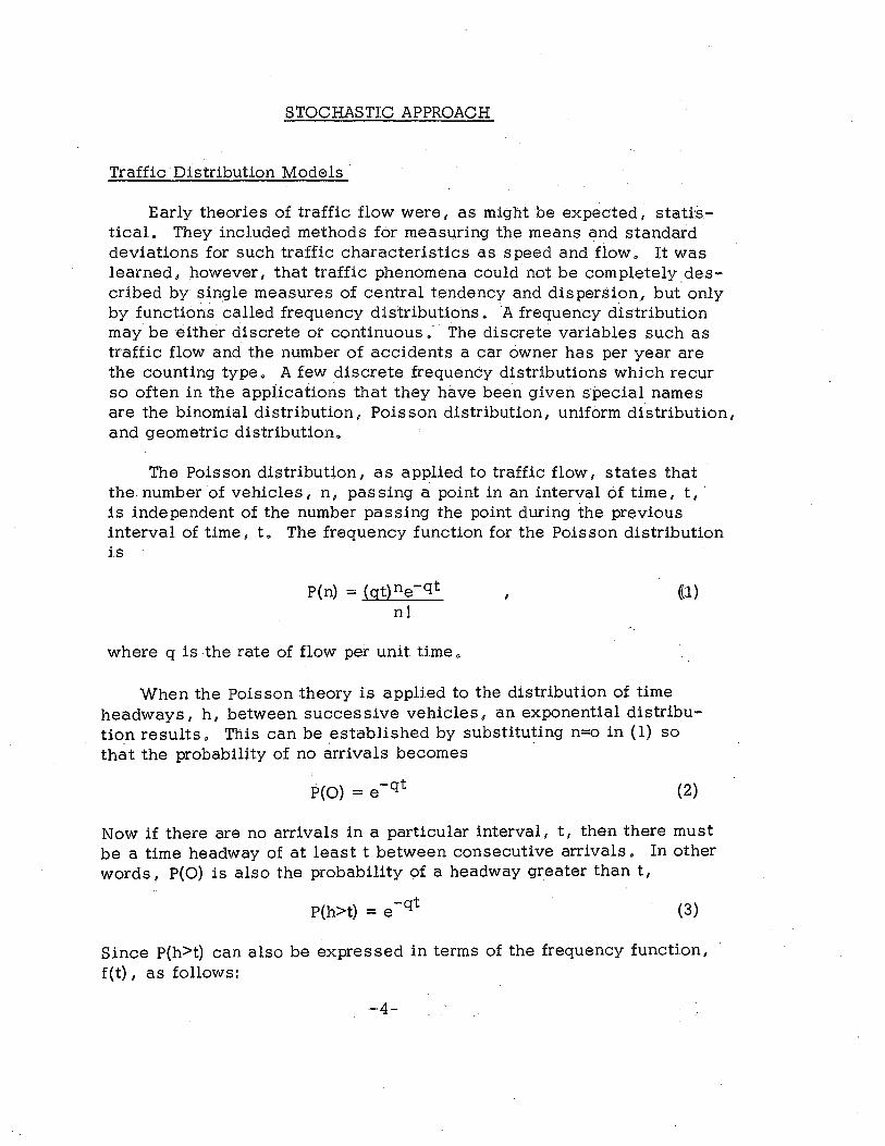
Early theories of traffic flow were 1 as might be expected, stati:s­tical. They included methods for measuring the means and standard deviations for such traffic characteristics as speed and flow. It was learned 1 however, that traffic phenomena could not be completely des­cribed by sin9le measures of central tendency and dispersion, but only by functions called frequency distributions. A frequency distribution may be either discrete or continuous. The discrete variables such as traffic flow and the number of accidents a car owner has per year are the counting type. A few discrete frequency distributions which recur so often in the applications that they have been given special names are the binomial distribution 1 Poisson distribution, uniform distribution, and geometric distribution,

The Poisson distribution 1 as applied to traffic flow, states that the number of vehicles 1 n, pas sing a point in an interval of time, t 1 ·

is independent of the number passing the point during the previous interval of time 1 t. The frequency function for the Poisson distribution is

P(n) = (qt)ne-qt n!

where q is the rate of flow per unit time"

«1)

When the Poisson theory is applied to the distribution of time headways, h, between successive vehicles 1 an exponential distribu­tion results, This can be .established by substituting n=o in ( 1) so that the probability of no arrivals becomes

P(O) = e -qt (2)

Now if there are no arrivals in a particular interval, t, then there must be a time headway of at least t between consecutive arrivals. In other words 1 P(O) is also the probability of a headway greater than tl

-qt P(h>t) = e (3)

Since P(h>t) can also be expressed in terms of the frequency function, f(t} 1 as follows:

-4-

(X)

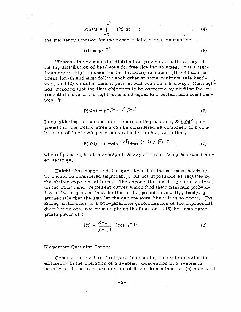
P(h>t) = l f(t) dt ( 4)

the frequency function for the exponential distribution must be

f(t) = qe -qt ( 5)

Whereas the exponential distribution provides a satisfactory fit for the distribution of headways for free flowing volumes, it is unsat­isfactory for high volumes for the following reasons: (1) vehicles po­ssess length and must follow each other at some minimum safe head­way, and (2) vehicles cannot pass at will even on a freeway. Gerlough 1 has proposed that the first objection to be overcome by shifting the ex­ponential curve to the right an amount equal to a certain minimum head­way, T,

P(h>t) = e-(t-T) I (f-T) (6)

In considering the second objection regarding passing, Schuhl.~ pro­posed that the traffic stream can be consid:ered as composed of a com­bination of freeflowing and constrained vehicles, such that,

P(h>t) = (1-a)e-tltl+ae-(t-T) I (t2-T) (7)

where f 1 and f 2 are the average headways of freeflowing and constrain­ed vehicles.

Haight3 has suggested that gaps less than the minimum headway 1

T 1 should be considered improbably, but not impossible as required by the shifted exponential forms. The exponential and its generalizations 1

on the other hand, represent curves which find their maximum probabi­lity at the origin and then decline as t approaches infinity, implying erroneously that the smaller the gap the more likely it is to occur. The Erlang distribution is a two:...parameter generalization of the exponential distribution obtained by multiplying the function in ( 5) by some appro­priate power of t,

f(t} =te-l (qc)ce -qt (c-1)!

(8)

Elementary Queueing Theory

Congestion is a term first used in queueing theory to describe in­efficiency in the operation of a system. Congestion in a system is usually produced by a combination of three circumstances: (a) a demand

-5-

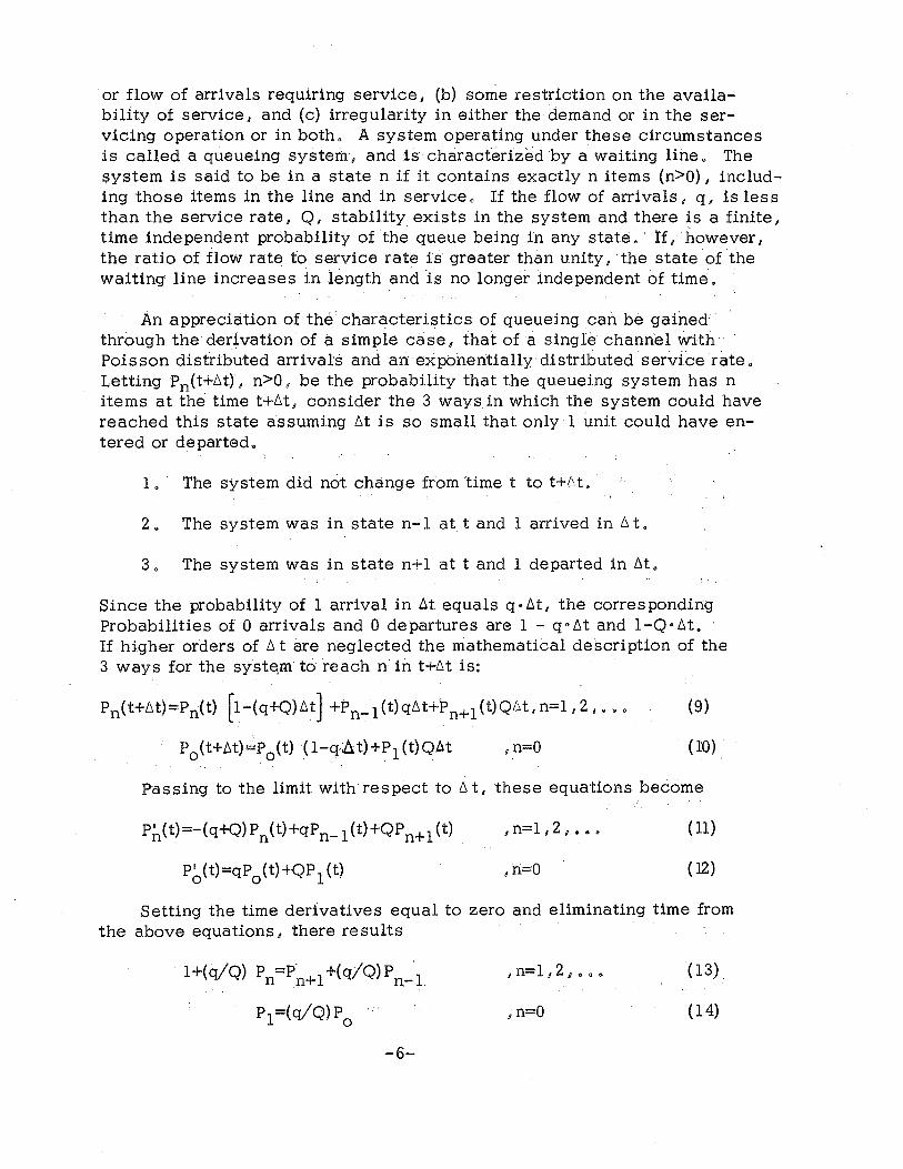
or flow of arrivals requiring service 1 (b) some restriction on the availa­bility of service, and (c) irregularity in either the demand or in the ser­vicing operation or in both. A system operating under these circumstances is called a queueing system·, and is characterized by a waiting line. The ~ystem is said to be in a state n if it contains exactly n items (n>O) 1 includ­ing those items in the line and in service. If the flow of arrivals, q 1 is less than the service rate, Q 1 stability exists in the system and there is a finite 1

time independent probability Of the queue being in any State o ' rc however 1

the ratio of flow rate to service rate is greater than unity, the state of the waiting line increases in length and is no longer independent of time.

An appreciation of the characteristics of queueing can be gained through the derivation of a simple case I that of a single chann'el with Poisson distributed arrivals and an exponentiallY' distributed service rate., Letting Pn(t+M) 8 n>O, be the probability that the queueing system has n items at the time t+Mo consider the 3 ways in which the system could have reached this state assuming .6t is so small that only 1 unit could have en­tered or departed.

1 . The system did not change from time t to t+M.

2. The system was in state n-1 at t and 1 arrived in 6 t.

3. The system was in state n+1 at t and 1 departed in M.

Since the probability of 1 arrival in 6t equals q·M~ the corresponding Probabilities of 0 arrivals and 0 departures are 1 - q•M and 1-Q·6t. · If higher orders of 6 t are neglected the mathematical description of the 3 ways for the syste,m to reach n in t+M is:

Pn(t+L'It)=Pn(t) [1-(q+Q)t.t) +P n- 1 (t)qL'It+P n+ 1 (t)Q6t8 n=18 2,. . • (9)

,n=O ( 10)

Passing to the limit with respect to L'l t, these equations become

P~(t)=-(q+Q) P n(t)+qP n- 1 (t)+QP n+1 (t)

P~(t)=qP 0

(t)+QP 1 (t)

8 n=1, 2 o •••

,n=o

( 11)

( 12)

Setting the time derivatives equal to zero and eliminating time from the above equations, there results

1+(q/Q) p n =Pn+1 +(q/Q) P n-1

P1=(q/Q)P o

-6-

1 n=1, 2 D o o •

,n=O

( 13)

{14)

where Pn is the steady state (time independent) probability that there be n units in the system., Letting n=l in (13) and substituting for p from (14) in (13) 1 equation (13) becomes · 1

(15)

Then solving (13) and (15) by induction, the queue length probabilities take the form of the geometric distribution ..

p n =(q/Q)n [1-(q/Q) J The mean of this distribution is

or E(n)=(q/Q) ( 1-(q/Q),] -l

E(n)= _g__ Q-q

where E(n) is the expected number in the system.

(16)

( 17)

Use of (17) will be illustrated by an example. Consider the op­eration of a single lane of freeway traffic at a toll booth. If the lane flowis q==;B,,Q,p,jiehioles per hour and the toll booth operator can process an auto in 4 seconds on the average, then

Q = 3600 seconds hour = 900 vehicles/hour · seconds vehicle

(18)

Thus Q, the service rate in a queueing system in general, takes on an added physical significance in the special case of a highway facility -that of 11 capacity .. " In most traffic engineering problems, an important consideration is the solution of a capacity-demand relationship.. Al­though it is recognized that capacity on the average· must exceed de­mand on the average, the importanC'e of the distributions of these para­meters is not generally appreciated.. Using the toll booth example this will be illustrated (see Figure la).

If it is assumed that the flow of 800 vehicles per hour representing the demand on the toll booth conforms to a Poisson distribution and that the rate at which the operator works is exponentially distributed then the expected number of vehicles at the toll booth is obtained from ( 17) •

E(n) = 800 =8. (19) 900-800

-7-

ARRIVALS ---~

< q = aoo·vph) 0 ' 0 0 0 0 0 0 ~

TOLL BOOTH

E ( n) = q I (Q- q) = 8.0

--~~ DEPARTURES

( Q =900vph)

(a) POISSON (RANDOM) ARRIVALS AND EXPONENTIAL SERVICE

ARRIVALS ___ ,.__

( q = 800 vph)

E(n)=q/Q=S/9

[Q] TOLL BOOTH

___ ,.__ DEPARTURES

( Q = 900 vph)

( b) UNIFORM (METERED) ARRIVALS AND UNIFORM SERVICE

COMPARISON OF THE EFFECT OF THE DISTRIBUTION OF ARRIVALS AND THE DISTRIBUTION OF SERVICE ON CONGESTION

FIGURE 1

On the other hand, if arrivals at the toll booth are constant (accom­plished perhaps through metering), and some uniform automatic ser­vicing device is utilized, the expected number of vehicles at the toll . booth becomes (Figure b)

E(n) = q/Q = 8jg

Two important conclusions may be drawn:

( l) The distribution of demand and the distribution of service (capacity} are important.

(20)

(2} The expected number in the system, E(n) is a measure of the inefficiency of a facility 1 or a quantitative measure of traffic congestion.

Queueing-Stochastic Models

The queueing-stochastic models are based on well established relationships between traffic flow theory and the classical subjects of queueing theory 1 stochastic processes 1 and mathematical proba­bility. A distinct approach to explaining the bunching tendency of moving vehicles on a highway is provided by a queueing approach. If constrained vehicles on a highway are considered as platoons or queues 1 then the Borel-Tanner distribution can be },Used as a model for the distribution of queue lengths. A queue is described by start­ing with a random position (or set of arrival times) of vehicles, con­sidering all vehicles within some distance S as being queued and then moving these queued vehicles back so that they are exactly S apart, at the same time including any more vehicles which are then within the distance of the end of the queue. The probability that a queue has exactly n vehicles is

n-1 P(n) = ........ n~· -

n:·! (Sk) n-1 e -Skn (21)

Miller4 hypothesized that vehicles may be considered as travel­ing in platoons or queues 1 where a queue may be of one or more ve­hicles. These queues are assumed to be independent of each other in size, position and velocity. The criteria for determining queues are that the time interval between queueing vehicles be less than 8 seconds and that the relative velocities be within the range of -3 mph to +6 mph.

-9-

Haight3 suggests an "Independent Traffic Queueing Model" as a particular instance of compound gap theory. The model is based on independent gaps and leads to queue lengths with geometric probabi­lities 0

Formulation of Moving Queues Model

As traffic volumes increase, vehicles tend to form platoons 8 or moving queues. The criteria for determining when two moving vehicles are queued is arbitrary. And 8 for that matter 1 the criteria for deter­mining when two stationary units are queued in classical queueing systems is equally arbitrary since the concept of distance did not ap­pear in the queueing derivation in the previous section 0 Borrowing from car-following theory 1 a line of moving vehicles could be consid­ered to be in a single queue if each must react instantly to the speed reductions of its predecessor 0 For the purposes of this discussion, it will be assumed that a vehicle is queued to the vehicle ahead iff_ its headw9y is less than S if space is the parameter, and T if timeiis the parameter.

There are several traffic characteristics that can indicate conges­tion on a highway facility: low speeds, high flow to capacity ratios 8

high space densities 8 and high time densities (lane occupancy) o It seems o however 8 that these various parameters ignore the distribution of traffic and therefore give imcomplete descriptions of congestion and the state of a systemo as exemplified in the toll booth illustration if only q a'nd Q are considered 0 It is suggested that E(n) (which o in the case of moving queues 8 shall be called the queue length or number queued) is a logical measure of congestion on a highway facility o just as it is in conventional queueing systems. Figure 2 illustrates how the moving queue length might be a more sensitive indicator of con­gestion than density,

' The formulation of the moving queues model is based on perform-

ing a Bernoulli test with probabilities p and (1-p) on each headway {either time headway or space headway)). If headways between suc­cessive vehicles are assumed to be independent, then the probability of having a queue of exactly one vehicle is

(22)

-10-

00 00 0 0 0 0

E(N) = 8/6 = 1.33

0 0

E(N) = 8/4 = 2.00

COMPARISON OF T·wo HIGHWAY FACILITIES WITH EQUAL DENSITIES AND DIFFERENT CONGESTION INDICES

FIGURE 2

where 1-p is the probability that the headway of vehicle number 2 (Figure 3a) is greater than the arbitrary queueing headway, S. Sim­ilarly the probability of a queue of exactly two vehicles is obtained by a combination of one 11 success 11 followed by a 11 failure, 11 or

P2 = p(l-p)

where p is the probability that the headway of vehicle number 2 (Figure 3b) is greater than the arbitrary queueing headway 1 S. By induction, the individual queue lengths form a geometric distribu­tion (Figure 3 c)

1 n=11 2 1 o o o

The expected queue length E(n) is given by

which yields

00

E(n) = L n Pn n=1

E(n) = 1 P1+ 2P2+ 3P3+ .•. = ( 1- p) ( 1 +2 p+3 p2 + ..• ) .

(23)

(24)

(2 5)

The second term of (2 5) is a derivative of a geometric series whose sum is 1/ (1-p) 2; therefore

E(n) = ( 1-p)- 1 • (26)

The probability (1-p) of any vehicle headway 1 X 1 being greater than the arbitrary queueing headway 1 S ,_is ·of course dependent on the distribution of vehicles in space on the highway lane,

00 .

1-p = P(x>S) =1 f(x;k~c)dx s

The two parameter probability distribution implied in (2 7) is the Erlang distribution. Substituting in· (2 7) 1

00

P(x> S) =I (kc) ~ . xc-1 e -ckxdx

8 (c-1 !

(2 7)

{28)

where }{ is the average concentration of vehicles 1 x is distance 1 and c=1, 2, 3, •. : Substituting (28) in (27) in (26) yields

-12-

STATE OF SYSTEM PROBABILITY OF OCCURRENCE

s

QUEUE LENGTH= I -b) .. ®

· I. x. .I P(X2> S)=l-p

(a)

s

QUEUE LENGTH= 2

r .. s IE 'I

~~~ x. t x, r p (1-p)

(b)

s

QUEUE LENGTH=n

t ..

-~r·····-~ t x. ~· [ x •• , • Pn-1 (1-p)

(c)

BERNOULLI TEST FOR DETERMINING THE PROBABILITY OF INDIVIDUAL QUEUE LENGTHS

FIGURE 3

[

OQ ] -1 . E(n) = l (kc) c xc- 1e -ckxdx

S (:c-1)! (29)

which is the fundamental relation between the moving queue length E(n), concentration (k), the arbitrary queueing headway S, and the distribution of concentration 8 c.

The theory was developed for space headways only. It is appar-. ent from the arbitrary nature of the queueing criteria that the arbitrary nature of the queueing criteria that the results can be extended to time headways by replacing x, S and kin (29) by t, T and q.

-14-

STUDY PROCEDURES

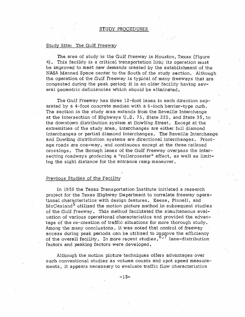
Study Site: The Gulf Freeway

The area of study is the Gulf Freeway in Houston, Texas (Figure 4). This facility is a critical transportation link; its operation must be improved to meet new demands created by the establishment of the NASA Manned Space center to the South of the study section~ Although the operation of the Gulf Freeway is typical of many freeways that are congested during the peak period; it is an older facility having sev­eral geometric deficiencies which should be eliminated.

The Gulf Freeway has three 12-foot lanes in each direction sep­arated by a 4-foot concrete median with a 6-inch barrier-type curb. The section in the study area extends from the Reveille Interchange at the intersection of Highways U.S. 75J State 225, and State 35, to the downtown distribution system at Dowling Street. Except at the extremities of the study area, interchanges are either full diamond interchanges or partial diamond interchanges. The Reveille Interchange and Dowling distribution systems are directional interchanges. Front­age roads are one-way 1 and COntinUOUS except at the three railroad crossings. The through lanes of the Gulf Freeway overpass the inter­secting roadways producing a "rollercoaster" effect, as well as limit­ing the sight distance for the :entrance ramp maneuver 0

Previous Studies of the Facility

In 1956 the Texas Transportation Institute initiated a research project for the Texas Highway Department to correlate freeway opera­tional characteristics with design features. Keese 1 Pinnell, and McCasland5 utilized the motion picture method in subsequent studies of the Gulf Freeway. This method facilitated the simultaneous eval­uation of various operational characteristics and provided the advan­tage of the re-creation of traffic situations for more thorough study. Among the many conclusions, it was noted that control of freeway access during peak periods can be utilized to improve the efficiency of the overall facility. In more recent studies 1617 lane-distribution factors and peaking factors were developed~

Although the motion picture techniques offers advantages over such conventional studies as volume counts and spot speed measure­ments, it appears necessary to evaluate traffic flow characteristics

-15-

~. SURFACE STREET

DISTRIBUTION SYSTEM

::·=···~ :·:·:·.-·~·A ::: ::::.~ ·X·:·. ·:-:·:·:·:· ').. .·:::. ·:::::·=·~UNG

SJSttW ........... ·.;:~1

AREA

::~:~·;ij): .. J i ·=:=:=:=:=:=~~=:=:=:=:=:~ ~ :·:·:·:·:·::·:·:·:·:·:·~1 "'-..... :::;;::::; NiMh • 4l~i :::::::2>~< 4"~~~~~~~z .. ·::.········'7 \; ,~~ I

/ H.B. 8 T. RR TELEPHONE WAYSIDE 7GS

~!; > l~ r,> ( \ <t' ~ 7 / < 5i ~~ = ~ I

STUDY AREA-GULF FREEWAY HOUSTON, TEXAS

FIGURE 4

by methods that do not rely on point survey data for describing flow characteristics over an area & Two methods that have been success.,­fully utilized are television camera surveillance and aerial pho'to­graphy o At this time a television surveillance system is being de.,­signed for the Gulf Freeway, but will not be operational for another year. Therefore, the application of data collection by aerial photo­graphy seems to provide the best means of evaluating the critical areas of traffic congestion.

Time-Lapse Aerial Photography

In September 1963, aerial surveys of the traffic flow on the six mile study section of the Gulf Freeway were initiated by the Texas Transportation Institute. Two types of aerial photography were inves­tigated: · ( 1) strip photography where two continuous pictures are taken simultaneously over the entire study section: and (2) time-lapse photo­graphy where individual overlapping pictures are taken at short intervals of time. The objectives of this study were to compare the two types of aerial photography.· As a result of this study, McCasland8 concluded that time-lapse photography is more suited for density and speed measure­ments. Moreover I the time-lapse method can provide multiple readings of speed for each vehicle.. From these several measures of speed, the acceleration of vehicles can be calculated.

The aerial surveys, from which the data for this paper were obtained~ were conducted by the International Aerial Mapping Company. Flights were made according to a predetermined plan. Beginning at the south end of the study sectionu the crew filmed northbound 4 circled upon reaching Dowling Street, then filmed the study area from north to south, circled at the south'extremity, and again filmed northbound. Three such repetitions were made; or a total of nine filming runs over the area, six northbound and three southbound. A precise time measurement was furnished indi­cating the clock time when the plane passed over the two limits of the study area. The plane was a Cessna 19 5 flown at 2400 feet. A 24-inch focal length aerial camera with a 60 percent overlap was utilized. The basic information concerning the aerial:;Stlic1Y:.is. ·s.umma'rized:.irt'T.able b'

Information Obtained

The traffic flow data wer;e taken off 18-in. by 9-in. positives with a scale of approzimately 1 inch to 100 feet and a 60 percent overlap, One­hundred-foot stations were located on the photographs and .vehicles were

-17-

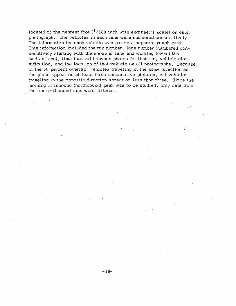
located to the nearest foot ( 1/100 inch with engineer 0 s scale) on each photograph. The vehicles in each lane were numbered consecutively. The information for each vehicle was put on a separate punch card. This information included the run number, lane number (numbered con­secutively starting with the shoulder lane and working toward the median lane), time interval between photos for that run, vehicle clas­sification, and the location of that vehicle on all photographs. Because of the 60 percent overlap, vehicles traveling in the same direction as the plane appear on at least three consecutive pictures, but vehicles traveling in the opposite direction appear on less than three. Since the morning or inbound (northbound) peak was to be studied, only data from the six northbound runs were utilized. -

-18-

TABLE 1

INDEX FOR TIME-LAPSEAERIAL SURVEY

Strip No o Direction Exposure No. Time of Run Time Lapse Start End (Seconds)

4 Northbound 1-49 6:45:37A.M. 6:48:20A.M. 3.40

5 Southbound 50-106 6:50:26 6:54:02 3.95

6 Northbound 107-146 6:55:32 6:58:06 3.95

7 Northbound 1-48 7:03:44 7:06:39 3.70

I 8 Southbound 49-94 7:10:53 7:13:30 3.50 I-'

<0 I

9 Northbound 95-141 7:15:55 7:18:34 3.45

1 Northbound 1-56 7:25:15 7:28:02 3.05

2 Southbound 57-107 7:30:25 7:33:38 3o85

3 Northbound 108-160 7:44:43 7:47:35 3.30

Distribution of Space Headways

Inherent in the formulation of the moving queues model is the hypo­thesis, stated in Equation 27, that the distribution of vehicles on a free­way lane conforms to an Erlang frequency distribution. This is

1 in fact,

a logical choice because the exponential distribution, well established in the description of traffic headways, may be considered as a special case of the Erlang distribution for which c=16 Moreover, use of the Erlang distribution for all values of c affords the opportunity of considering the disttibution of vehicles for all cases between randomness (c=1) to complete uniformity (c=r) •

Using the aerial surveys of traffic flow over the study area of the Gulf Freeway iffHouston~ the distribution of space headways for lane 1 (shoulder ?lane) is summarized in Appendix A. These constitute thef'ob­served" distribution, and the inference is then made that the postulated theoretical (Erlang) distributi.on is in fact the true distribution. "

The use of the. Chi-square test as an index of the goodness of Ht of observed and expected frequencies of occurrence is well established in testing such an hypothesis. The value for the Chi-square is simply the summation of all the deviations between the observed (f) and expected frequencies (F) squared.and divided by the expected frequencies.

J

x 2 = L (fi-Fi)2 /Fi (30)

i=1

where j is the number of possible outcomes. Thus if an experiment is performed repeatedly o the distribution of the quantity in (30} will approach that of the x 2 variable with j-1 degrees of freedom. Since the x2 distribu­tion is only an approximation to the exact distribution~ care must be exer­cised in the application of the Chi-square test. Experience indicates that the approximation is usually satisfactory if fi>5 and j>~. If j<5, it is considered advisable to have the fi somewhat greater than 5. Thus, if the expected frequency of a group does not exceed 5, this group should be combined with one or more groups.

When the Chi-square test is applied to groups with probabilities which de pend on unknown parameters, as in this problem, the number of parameters defining the distribution are subtracted from the degrees of freedom. Thus, for the test of distribution of space headways based on i>c.

the Erlang distribution., the degrees of freedom become: d.f.=j-3.

-20-

The organization of this phase of the investigation suggests 24 Chi-square tests per lane per flight trip.

Determination of Queueing Variables

Once the distribution of headways has been established 1 the que­ueing model must be verified. The moving queues model states (see Equation 29) that congestion as exemplified by the average length of queue varies inversely with the percentage of large headways, or di­rectly with the percentage of small headways for a given concentraion 1

k.

Integration of Equation 29 for c=l$ 2 1 3 1 and 4 yields the following:

E(n) =ekS c=1

2kS E(n)c=2=~

2kS+1

E(n)c=3::::; e2kS 4. S(kS)2+3kS+1

E (n) c=4= e4kS 10.6 7 (kS) 3+8(kS) 2+4kS+ 1

(31)

(32)

(33)

I (34}

where E(n) is the expected length of queue, k is the concentration of vehiCles 1 and S is the arbitrary queueing headway. The implication here is 1 that use of the first four curves of the Erlang family will be sufficient to provide a satisfactory fit to the varied conditions of con­gestion experienced on a long busy freeway.

Iri order to check the relations in the equations 31 through 3 4 1

headway measurements were performed on the same aerial photos used to find the distribution of headways. Observed queue lengths for the value of 8=1 00 feet are given in Appendix B.

-21-

RESULTS

Stream Characteristics

Because of the design and markings of the highways, and the driver~ s -experience, the traffic stream tends to become separated into lanes of flow. The principal charactei:tstics associated with the traffic stream are the trans­verse distribution of vehicles and the longitudinal distribution of vehicles ..

The transverse distribution of vel\icles may be expressed as a percent­ageD either in terms of lane occupancy or lane usage.. Lane occupancy, as used here$ refers to the relative lane densities over short lengths of freeway~ Figure 5 illustrates the percentage of vehicles occupying each lane at two times during the morning peak~ The times chosen correspond to operation just before congestion (7:05AM): .al).d just after congestion (7:15-AM). At 7:05 AM there are definitely less vehicles in the shoulder lane than in the other two lanes. Since this phenomena is even more pronounced in the areas immediately preceding entrance ramps 1 such as at the Woodridge, Way­side, Telephone and Scott Interchanges 8 it is apparent that drivers are avoid­ing the shoulder lane because of the entrance ramp traffic. In the vicinity of the Reveille Interchange; however 1 the presence of a left-hand entrance ramp causes this phenomena to appear 1 not on the shoulder lane, but on the median lane. Mter congestion sets ins occupancy on the shoulder lane drops to even a lower-percentage in many locations ( see Figure 5 7:15 AM}, but rises abruptly immediately downstream from such busy entrance ramps as Griggs, Wayside, Telephone and Cullen.

Although occupancy represents a means of evaluating lane performance, it is probably less effective$ and certainly less conventional, than lane usage as a figure of merit. Lane usage .. as a parameter, considers speed as well as density, and is analogous to volume or flow.. In Figure 6 the percen­tages illustrated represent the lane distribution of calculated volumes ob­tained by multiplying speedby density over 700-fo_ot sections .. The data for 7:05 AM indicate that the median lane handles 'the highest percentage of flow for most of the freeway with the center lane a close second. At 7:15, the shoulder lane seems to suffer additional losses. In the vicinities of Telephone and Cullens this drop in the percentage of the shoulder lane vol­ume must be attributed to reduced occupancy rather than a reduction in speeds, as seen by comparing_ Figures 5 and 6.

Two important conclusions may be drawn from the analyses of the trans­verse distribution of vehicles: ( 1 ) the shoulder lane is the least efficient lane both in terms of occupancy and throughput, due to the entrance ramp geometries and aggravated by the effe::ct of the high percentage of trucks on that

-22-

lane , ( 2 ) the shoulder lane suffers the highest fluctuations in occupancy and flow and therefore seems to be the most sensitive to geometric and operational peculiarities.

The longitudinal placement of vehicles in the traffic stream .also affects the driver 1 s choice of speed, and is to the driver the primary indicator of impending congestion. The linear measurement of headw{;iys between suc­cessive vehicles does, it has been shown 1 give the number of vehicles along a traffic lane and is., therefore, a direct measure of density. Actually~ varia­tions of space headways in a traffic stream may range from a few feet (the vehicle n s length being the lower limit) to several hundred feet under conditions of free flow.

The natural distribution of vehicles in the traffic stream cpn be extremely useful in explaining the operations of many facilities.& Several traffic dis­tribution models were considered before the Erlang frequency distribution was hypothesized as the natural distribution of vehicles per lane.. In order to obtain the expected frequency of space headways over individual sections of freeway, cumulative frequency curves were plotted for the first four Erlang curves ( c = 1, 2, 3 1 4 ) (see Figure 7 ) • The observed frequency of space headways for the shoulder lane is summarized in Appendix A. The shdulder lane was chosen for this investigation both because of its influence on ramp operations and its sensitivity to impending congestion. Figure 8 illustrates a comparison of the observed and predicted values based on the Erlang hypo­thesis. The true distribution is obviously "two-tailed~" and the 11 one-tailed" exponential distribution curve :( c = 1 ) gives an extremely poorfit. In Table 2 0 the results of 140 Chi-Square tests are summarized. The freeway areas tested., represented by three photos, cover approximately 1 mile.. It is of interest to note that the exponential distribution ( c = 1 ) . 'if\(as rejected; (indicated by an asterisk) 8 as expect'ed, in almost every case. However, in only four of the thirty-four locations tested in Table 2 was it impossible to fit one of the Erlang curves:.to :observed data.

In order to obs~rve the variations in the natural distribution of vehicles in time and space, th;e Erlang coefficient of randomness 1 c~ values providing the best fits to the o~served headways were plotted in the form of contours (Figure 9),. It is apparent that as the freeway becomes congested., the dis­tribution of vehicles becomes less randon{~ tending toward uniformity., Also1

some combinations of geometric features tend to reduce randomness in the traffic stream$

-23-

I.SG.N.RR SCOTT ST. CULLEN H.B. ST. RR DUMBLE H.B.ST.RR TELEPHONE

______ , ...... --... ______ ,--, __ ~.-::[17 Lone7 7:05A.M, ,,

40 Cenrd ~Lane....- -... ,

......... ~ ~SJ. ovlderL ', .:::.---......../ ~ ............ --r_---f---- ...........

~ -----:::--- ---~---~~ '7ne --- '--~ ...__? -------- -- ---~

~~ 30 - ___., --~,~-- ' ------- -- ____ ,_.......

~~ ....... ...--_ _..........:::: ----- !-

7:15A.M. I

~l I '

I 40 f---· ·- --- ! -~----- ----

::::---......: --- _::_---- :.:::.-:=::: -- -;::..."----- ......... ---- -------- --::,:;.---..: ~ 0 ---- --·- _,....... -- -- ------- ----~-=.::..---=== ,_,__._---· ~~ 30 --------- ..... -· -.---- --------

~--.....____... / -- -.....__r--- ~ -- -d:~ -STATION 20 30 40 50 60 70 80 90 100 110 120 130 140 150

\WAYSIDE BRAYS BAYOU GRIGGY L -r·· ~ "v'~ r~ l - /

" -·, / ""' ~ l ./ 1' J P' ~Cj/ - \ I ~,/-....

7:05A.M ------- - .4.0 -- -- -- - -- --- _,. --- ---r--. ~- -- ::::-:::> ~ 1'--... --~ ------- ~-----:::< ----=-=-.:. ...... -=---==-==-~_;_ ____ __ ":::-::-...~- --.... ._---- --- -,

~- -"---- -- ....... _ >< 30 --- -- --- ......... /-r----................. _!_......

7:15A.M. ' ' I ,r<~cwlde ~Lane ' 40 = =·--~

~----......... ~:: ;::.;-<---- -- C>< --- ~.....::.:::. ~S-n~ -- V- ----~ --- ---- ______ :-;:;

_ ... -- ce~ ~_:::;.;>~f':----- -- ~-30 ./ -- --r------- ---- - -- ............... _ -f--.:::::-~ ~nldne

' ' 160 170 180 190 200 210 220 230 240 250 260 270 280 290 300

- ~~--·-~-- ------------

LANE OCCUPANCY

FIGURE 5

I. S. G.N. RR SCOTT ST. CULLEN H.B. aT. RR OUMBLE H. B. aT. RR TELEPHONE

~\I ~

BRAYS BAYOU GRIGGr

1 7:05A.M ~-·--r-·----'-.0-·-'·----r·-·· J! ______ ...__ ----- I -- 40' -- t-:.::::.:.::.-< ------ --;z-- ____ ,_ ____ --·----·;t: . J --- -- I

I--_ -- ... !"-~ -- -- ----- -- --- t--.. / ...... --- -=~.-=::::.:--- - ,-- ------ --- --- - -- ---- , -- ----~-=--c:::::: -- I 1-· ---+ . ..., ·- :30 I --- I ' I I l l I I - I

I , '

_i_ __ --~~ ~--- -- ~- I !Tt5AJ1lt ____ - ----- j ----::~-~~:t/~e, ~- 401 --I -=---== -- ---- ----- - ---==- I --- --------,;;.--------~I . i ' _.::.r ---,---.:. I I ,..::::;::::r--...-"'<...... ! ____ ___._.I .. --- . .- · ~SO

!--"" -~--" ........ - / -~ 1 t--.- -- ~~~~J~ C=!- ~~e,~kt?e "::~qq~.~f.~~~L~~· .. ,J j

160 170 180 190 200 210 220 _____ 2~--- .. J!40 250 260 270 280 290 300

LANE USAGE

FIGURE 6

.99

.98

jn .95

z <( .90 :I: 1--a:: .80

~ .70 <:{ w.so a:: (!) .50

~ 40 s:· 0.30 <(

~.20

~ .. 10 m 0 s: .05

.02

.01

..............

.............

~ ~ ~

............. ...........

"--.. ...........

............. r-----~ r-......

~ .......... "" ~ ~ "" ~ t:' "" """ ~ ~ t--..: t'--.." I'..

R3 s:: r-0: i". f": ~ 0

""\ ~

"'

~

~ ~ ~ ~ ~0

""" i".~ f"'-.

~ ~""' ""' ~~""" ""' """ ~ ~

""' ~ f\_ '\ ~

' ~\ ~ 1'\.'\. \ [\\

" "' "' 1\ l\

.99

.98

jl> .95 z <( .90 :::r: 1--

.80 a:: ~ .70 <:{ w .60 a:: (!) .50

~ f!JO 3 a .30 <(

~.20 LL 0 .10 ai 0 a:: .05 a..

.02

.01

I~ .......... !'... I

0 ""' -........

" T

" ~ ~ " ['..,r--., ~

~ ~ ~ " [',. r-..."' ~ ~ ~ ~ " r---.1'-. ~

""' 1'-.

0 1"-

~ r0 ~ ~ " ~f ~ 1'-.

'~ 0 !"\ '\ " ~ '\ " '\ ~ '" '"" "\"0" " " '\ D( '\ '\ '~~"'- \ \ '\ [\ ~ ,~\ \ 1\ '\ ~ ~\\ b\-- 1\\ 1\

..

I~ ~\\ [\\ \ ~\' ~\ 1\ I\ ~~ ~\ 1\

20 30 40 50 60 80 100 200 300 500 20 30 40 50 60 80 100 200 300 500

.99

.98

=(./) = .95 z <( .90 :I: 1--a:: .so w !;:t .70

~.60 (!) .50 >-: ~ 40

~.30

~.20 LL..

~ .10 m ~.05 Q..

.02

.0 I

"'-" ~ ""'"' ~ ~ ~ ~ ~ '\

SPACE HEADWAY, S (FT.) C=l

""' ~

""' ""

""' 1'\ 0

""' "' "" ~ ~ ['\ "' " ~ 1\. "'

0

~ '\ 1\'\ 1\. '\

'\ 1\ l\

1\\ 1\ 1\\ \ ~0 \ '\ I~ l\ i'\\ [\ [\ \ [\ 1\

r-._\ 1\\ 1\ "\~ \ \ \1\\ 1\\ \\ \

\\ \\ ,\ ~o\ \ ~ ~ l\\\\ 1\\ 1\ ~\\\ \\ \ \

"''\' \\\ \ \ \\\ \\ ~\ ~

.99

.98

:(./) .95

z <( .90 :::r: 1--a:: .80 w 1- ]'0

~ .60 a:: (!) .50

~ :40 0.30 <(

~.20 LL

~ .10 m ~ .05 a..

.02

.01

"'" ~ 1'\\

~ h\\ ~ ~ ~

\

SPACE HEADWAY, S(Ft) C=2

" "' '\ 1'- ~ 1"'- 0

'\ I\ '\ '\ 1'\ 1\ 1'\ 1\

k\ 1\ I\ 1\ ~ 0 \ 1\\ !\ I\ 1\ \ 1\ l\\ l\ I\ I'\ \ ~ \ \ ~\ lj ~ ~~ ~~ 1\ 1\

,\ l". ""~ ~.., \ ~ \l\ 1\l\ \ \ \ \ \

I\ [\""'\ l\~-"" \ 1\ 1\~ ~\ \ \

\ 1\\ '\ \ \ \ \ 1\\,\\ \\ \ \\\\ 1\\ 1\

20 30 40 50 60 80 100 200 300 500 20 30 40 50 60 80 100 200 .• 300 500 SPACE HEADWAY, S (FT) SPACE HEADWAY, S (FT)

C=3 C=4

CUMULATIVE PROBABILITY CURVES FOR THE ERLANG DISTRIBUTION

('-(kc)cxc-1 e-ckxd .) slc-IJ! x WHERE k = DENSITY(V.P.M.)

FIGURE 7

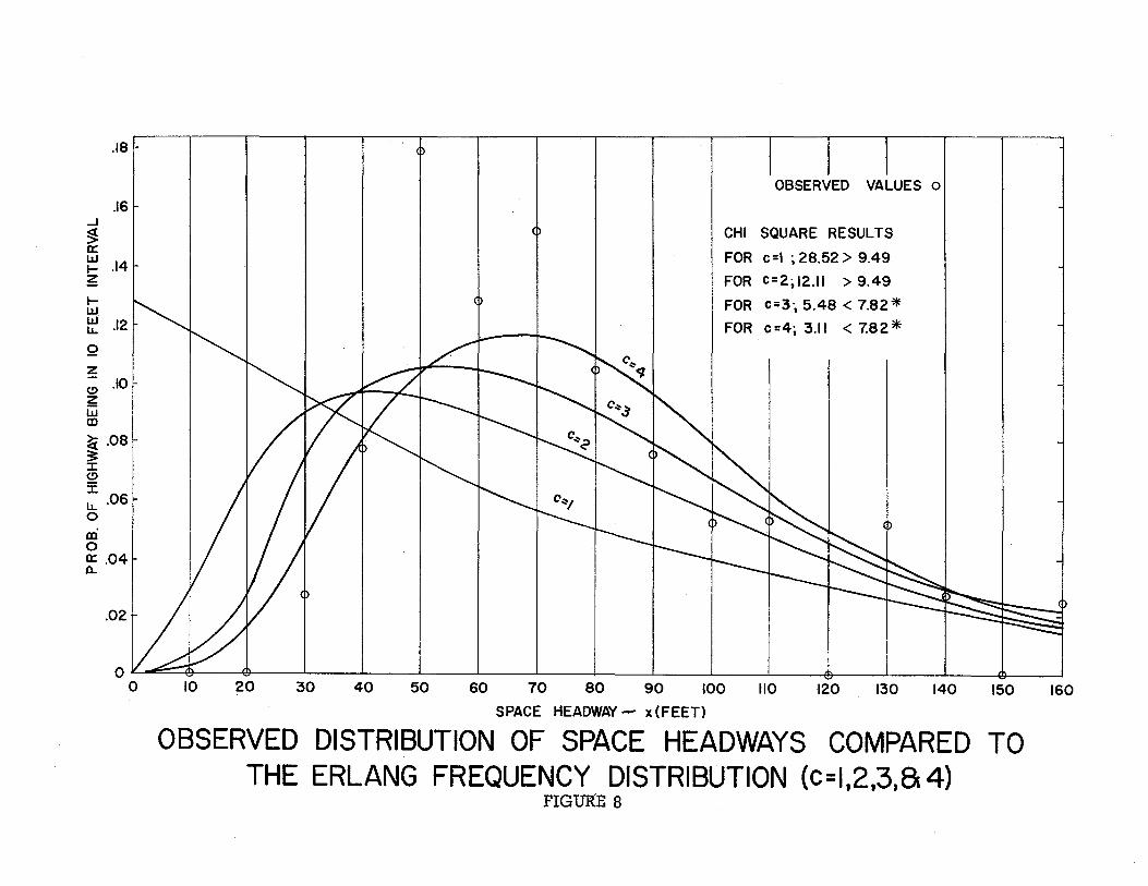
.18

.16 ...J

~ 0: UJ ~ .14

1-UJ UJ u. .12

Q

z (!) .10 ~

~ ~ .08 3: :c (!)

J: u. .06 0

a:i 0 0: .04 0..

.02

OBSERVED VALUES o

CHI SQUARE RESULTS

FOR c =I ; 28.52 > 9.49

FOR C=2; 12.11 > 9.49

FOR c=3·, 5.48 < 7.82 * FOR c=4; 3.11 < 7.82*

0 II'~ @ I I I I I I I I I 4> I I 0 I 0 10 20 30 40 50 60 70 80 90 100 110 120 130 140 150 160

SPACE HEADWAY .... x (FEET)

OBSERVED DISTRIBUTION OF SPACE HEADWAYS COMPARED TO THE ERLANG FREQUENCY DISTRIBUTION (c=I,2,3,S 4)

PIGUR:E 8

TABLE 2

SUMMARY OF CHI SQUARE TESTS FOR DISTRIBUTION OF HEADWAYS ASSUMING AN ERLANG DISTRIBUTION

Photos C=1 2 C=2 C=3 2 C=4 D.F. X D. F. x2 D. F. X D.F. x2

Strip 1 8,10,13 10 118.08* 12 50.34* 11 42. 78* 10 45.07*

14,17,20 6 52.29* 5 2l.01* 6 11.16 4 9.49 21,24,27 5 39.36* 3 8.92* 4 4.84 4 10.96* 28,31,34 4 24.30* 3 25.21* 2 2.77 2 2.36 35,38,41 2 17.33* 2 5. 72 2 6.18* 2 4.17 42,45,48 2 15.69* 2 7.02* 1 3.23 2 2.95 49,52,55 1 13.14* 1 l.35 1 l. 72 1 l.99

Strip 3 115' 118' l21 2 93.24* 2 124.75* 2 37 .50* 2 11.6o* l22,125,l28 4 46.23* 5 18.04* 5 9.11 5 5.94 129,132,135 4 35.14* 5 1l.23* 4 5.89 4 2.70 136,139,142 2 30.25* 3 8.23* 3 4.30 4 8.53 143,146,149 1 15.03* 1 5.63* 1 4.51* 1 6.78* 150,153,156 1 10.27* 1 4.64* 1 5.39* 1 2.05

Strip 4 6,9,12,15 1 0.97 1 2.08 1 4. 75* 1 7.60* 16,19,22 1 3.37 1 5.76* 1 4.14* 1 10.72* 23,26,29 1 6.19* 1 6.47* 1 3.03 1 4.26* 30,33,36 1 9.21* 1 0.66 1 2.06 1 6.27* 37,4o,43 1 15.68* 1 0.87 1 l.47 1 4.25*

Strip 6 116,119,122 1 21.30* 1 l.05 1 L85 1 5.31* l23,l26,l29 1 1l.85* 1 l.83 1 l.45 1 2.63 130,133,136 1 14.61* 1 4.99* 1 2.80 1 l. 70 137,140,143 1 7.64* 1 0.56 1 l.69 1 2.37

Strip 7 6,9,l2 5 31.80* 4 21.10* 4 7.80 4 l2.09*

13,16,19 1 -9.32* 1 5.22* 1 l.01 1 2.21 20,23,26 1 21.36* 1 8.21* 1 2.88 1 l.51 27,30,33 1 10.90* 1 2.90 1 0.44 -1 0.46 34,37,40 1 10.45* 1 2.55 1 0.82 1 l.07 41,44,47 2 13.51* 2 8.91* 2 5.37 2 13.09*

Strip 9 97,100,103 2 57.14* 5 35.69* 4 14.15* 4 9.00

104,107,110 4 37.98* 4 21.22* 5 3.79 5 3.37 111,114,117 5 4l.32* 4 18.45* 6 14.98* 5 8.02 118,121,124 3 40.22* 4 26.09* 3 16.33* 3 7.04 l25,l28,131 2 14.l2* 2 4.97 2 6.54* 2 9.67* 132,135,138 2 l2.48* 2 7.29* 2 11.28* 2 1l.07*

I.S G.N. RR SCOTT ST. CULLEN H.B. aT. RR DUMBLE

~\\ ~

LONGITUDINAL DISTRIBUTION OF VEHICLES IN TERMS OF THE ERLANG COEFFICIENT OF RANDOMNESS (LANE 1)

FIGURE 9

H. B. ST. RR TELEPHONE

25

.... t::

........

11.1 20 ~

11.1 ::::> 11.1 ::::> 0

0::

~ 15

en 11.1 ...1 2 :I: 11.1 > LL. 0 10

0:: 11.1 CD :E ::::> z 11.1

~ 5 0:: 11.1

~

00

I

OBSERVED VALUES 0

I

l~ r c (k c) c-1 -ckx

E(n)' ~ (c->J! X ,e dx FOR S=IOO FEET.

16 10

19

10 20 30 40 50 60 70 80 90 DENSITY ...... VEHICLES PER MILE -k.

OBSERVED RELATIONSHIP BETWEEN QUEUE LENGTH AND DENSITY COMPARED TO THE THEORETICAL RELATIONSHIP

FIGURE 10

6 0

100

Stochastic Model Parameters

Where the ;smooth- flow of traffic is interrupted by some form of bottleneck, the downstream, flow of traffic Will usually take the form of "platoons1 " or "moving queues." Obviously, if all vehicles using a freeway lane were ,equal-

" ly spaced, determination of the point of incipient congestion would be a simple matter. Thus, a second criteria for the formation of moving queues de­pends on traffic demand~ Because the motorist recognizes congestion as com­prising his right to choose his speed and his traffic lane 1 the natural tendency for groups to form and increase in length affords .a:.lpgical'.iridex of copgestion. It was suggested in the theoretical development of the moving queue concept that the expected number queued, E(n), represents a measure of congestion on a highway facility 1 just as it does in classical queueing systems.

The fundamental relation between the moving queue length, E (n) 1

and density 0 k, is given by Equation 29~ In Figure 10,. this equation has been· plotted for values of c= 1, 2, ,3~" and 4 1 using a space headway of 100 feet as a basis for the queueing criteria. The observed points numbered 1 to 19 refer to consecutive 1/3 mile lengths of the shoulder lane starting from station 300 to station 20. It is apparent that the observed relationship be­tween queue length and density compares very favorably to the theoretical relationship, and that for the shoulder lane of the Gulf Freeway1 the first four values of the Erlang "c" are sufficient to explain this queueing phenomena.

In Appendix B, :observed queue lengths are given for each photo of the six flight runs. It is apparent that1 consistent with the other congestion para­meters discus sed 1 moving queue lengths vary in both time and space. In order to effectively portray these variations 1 the contour format was aga.in utilized. In Figure 35, platoon, or moving queue lengths are illustrated in the form of contours.. Since the ordinate is time during the morning study period and the abscissa distance corresponds to the entire length of freeway,. the formation of platoons is completely documented.. Thus 1 at rstation 272 in the Reveille Interchange it is seen that the expected platoon size is 3. 0 vehicles at 6:58AM,. and that by 7:05 the average platoon length has tripled. Only the shoulder lane has been considered because of the conviction that this lane, due to its strategic location with respect to entrance ramps, is the real congestion barometer ..

-31-

1.6 G.N. RR SCOTT ST. CULLEN H. B. aT. RR DUMBLE H.B.ST.RR TELEPHONE

~\\ ~

~ ~~ (/ "', "--...:._ \ '~.G./ '--::z.o-....- 7 ~-\ \ \ \ '-:. . /"', ........ ....... . .......... '\... l i ~ 7 .. ~5 I -........ ............... ......... - --- / I I ~ . ;---~.0- _./ //1;:'-o-:> ':::;:- '\ -- r- -3.0-- -..> / I/ ' '1. 25 __ \'-. - ·' r ....._ /, / :1::·- _... ~ . -').0 ...__ -.- . . - / / - ,... ~ -......i ( -.__ '---:o-- _/ ' '-:z.o---r-, t' ( ('' ..--,.- --"-1 '1"15 r- / ---- ''- . .,/"'

'o . 1 I --r--.... ....--..... '- 1 '-...._ ---4.o--....{....-/ I ( ... -- --..--~.o I 7"05 ) --~ ., ' -- ' _.,In __

IV . . ~/ .I -z.o -z.o- ~ . "- I I ~ !

"' .... -:z.o-- I 1 ''-... 1 , . / \ ..... . i

\~ "'-'35 / \ -r .J ~ / ' -.......... /.,,, oo L.. ~~ ...,..,..r--_J•$2-. -----,..., ---:-- -;---,...,..,~' 0

STATION 20 30 40 so so 10 80 90 100 110 120 130 140 1so I

WOODRIDGE \WAYSIDE BRAYS BAYOU' GRIGGs; L "VE":j/~ ~ rl ~ '-f 2

' / -~z: ( \ >- s l z -e, I c_yp

- ---~- , _/ L I .-i-4-.o, '-, } 'I '.\ \ l I J J / j \4o.o- / 1 -.. \\ \ .L

1/ \. IS)' 1J~ /\ I I// -~.o- --" I \ 6l, "'\,0

. / r"·"', '. \ 1 t 1 ) ! v ! _,_ _, \ -1-~5

r--.... • / / / . \ \ 1 1 } 1 I { // I /// - -:zo.o- --- ....--. \,. \ ...._ I --: o- /I i } / I \. / 1 t' // ---1o.o- / I \ .4o.o -- .15 r--- ...,....- / .?_.-;;..:-....- ~~ I / '-- '· ! t / ·' - / / _v -- . r-- - 1 ,if!.-- :z.o.o / I / 1\ '- '--. , -- / /-;:::= =- ~::- I v· r' /

Ill /' '\ / ./ / I '· '-. .._ '- _, /" _,. -....- :-...... I \... 1"15 ----- r- ~~ ......... _ ... ....-/ 1~/ ....-....--- -:--"'\. ..... __ ...... ~ - ' - -f!.0-~-0/ """~ "' '·' ----'-----l .

r--,. -.::::=~~--~~- \_., -f::;-~~~:§~~===--=-====--==-s.o/ "- ",~,..._...::::::::.:::; -==-=---:;...--:::::..--~. . ' / ' --~]:.:: .- -~-- -- -- ---;:I :OS I ' - ..._20....-- " '.....:::: ......... --,;:::""'--:....... ------ 1 -- . , __ ,f.::::--.=-::- -

---- ---.. --- _,1,.55 - --- 2fO - / · ~- I /' --._/ / -;:-. 1.0

I I I 1 / 1 ... " ,I ' I ff' ~~~. ~~w.~~ ---160 170 180 190 zoo 210 220 230 240 250 260 270 280 290 300

PLATOON (MOVING QUEUE) LENGTH CONTOURS

FIGURE 11

APPLICATION

Freeway Surveillance Systems

Since the advent of the auto, forms of traffic control have been deemed necessary to maintain order and provide for safe, efficient operation. At intersections where the desire for safe movement is compromised by the available road space, the right of way is fre -:u quently alternated systematically between the conflicting flows. The most positive control device for achieving this assignment is the traffic signal, resulting in a stop-app-go driving pattern which con­tributes to highway congestion and driver frustration.

The advantages of the freewai are maintained only when the facility is operated under free flow.ing eruditions. One key to im­proving urban freeway operation lies. in increased surveillance. In its most basic form I urban freeway surveillance is limited to moving pt.Hf~;ffi~ •' Recently, helicopters have been used for fre~.way sur­veillance in Los ~ngeles and. other communitie-s. Efficient operation of high density freeways is 1 however 1. more than knowing the loca­tions of stranded vehicles; it may require closing or metering entrance ramps 1 or excluding certain classes of vehicles during short peak periods. Therefore I what is needed is a reliable 1 all weather source of surveillance information with no excessive time lag.

The broad concept of coordinated surveillance is usually referred to as traffic surveillance systems. In developing the Holland and . Lincoln Tunnel Surveillance Systems 1 the Research Section of the Port of New York Authority 9 stated: "Traffic surveillance systems consist of all the equipment and men needed t9 keep traffic moving. This in­cludes men and equipment to det~ct and measure continuously the main characteristics of traffic flow; to d·ecide what action is needed to maintain good traffic movement; to control traffic routing 1 speed, flow and/ or density; and to rectify conditions interfering with good traffic movement. "

Experimentation with closed circuit television as a surveillance tool was initiated on the John C. Lodge Freeway in Detroit. This offers the possibility of seeing a long area of highway in a short or instantaneous period of time 1 made possible by spacing cameras along the freeway so that a complete picture can be obtained of the entire section of roadway. Evaluation of the freeway operation de­pends mostly on the visual interpretation of the observers. However 1

-33;...:

many traffic people believe that this is not enough. The Chicago Sur­veillance Research Project, for exa,mpleu is predicated on the assump­tion that trained observers offered no uniform objectivity. In other wordsu if an expressway is operating wellu this quality can be detect­ed by observing operating characteristics. When the characteristics drop below a predetermined level, action may be taken. Although some attention was paid to the early investigation of the various traf­fic flow characteristics to determine which characteristics could be most useful to display the ,quality of operationu "the selection of para­meters to be measured.was tempered by thr

0limita.tions o~ the ma~m­

factured detecticm eqUlpment livailable~ " . .. Sim1larly D. 1n descnbing a proposed surveillance system on the Seattle Freeway u Cottingham defines the basic equipment requirements as consisting of instantan-. eous density measuring computers. ·The point being made here is that so important a decision as the choice of a control parameter should not be made by decree ..

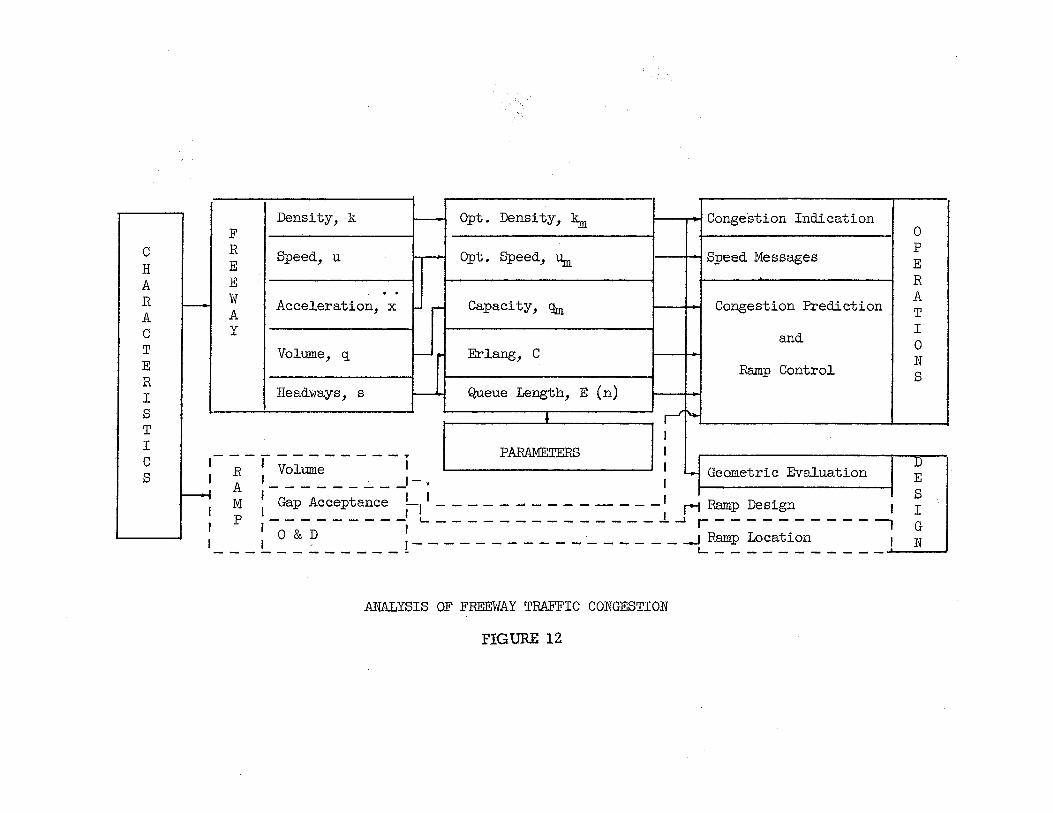
A traffic surveillance system should involve the continuous sam­pling of basic traffic characteristics for interpretation by established control parameters, in order to provide a quantitative knowledge of operating conditions necessary for immediate rational control and fu­ture design. This is illustrated in the form of a flow chart in Figure 12. The control logic of a surveillance system~ or any system., for that matter· is that combination of techniques and devices employed to regu­late the operation of that system. The analysis shows what information is needed and where it will be obtained. Theno- and only "then, can the conception and design of the processing and analyzing equipment neces­sary to convert data into operational decisions and design warrants be described. The solid lines in Figure 12 represent the portion of the to­tal research covered this year and the dashed lines indicate suggested future research. The three vertical blocks correspond to data collection and reductionu the contribution of theory 1 and the application of results in the broad areas of operations and designo

Congestion Prediction

In referring again to Figure 12, three of the five control parameters shown are excellent indicators. of congestion. ·These are optimum density, optimum speed and the ucritical" queue length. The critical queue length is obtained by choosing::JeS-iih the queueing equations equal to unity. Thus o

the values for the critical lengths are functions of the coefficient of random­ness.r c; and are 2.72 0 2.47 1 2 .. 36 0 and 2.21 for c:=l 1 2, 3, and 4 respectively.

-34-

c H A R A c T E R I s T I c s

Density, k r-- Opt • Density, k_m Congestion Indication F 0 R p

E Speed, u ,..... Opt. Speed, 'Um Speed Messages E

E R w . . A

f----1 A

Acceleration, x r- Capacity, CJm Congestion Prediction T y

and I 0

Volume, q ~--r Erlang, C N Ramp Control s

Headways, s t-'1 Queue Length, E ( n)

~ I

- - -- -- -- - - - - . I PARAMETERS I I y u ~---, 1 R

1 Volume I 1 Geometric Evaluation E

I I J-, I I • A --------- s r---t I II I · M Gap Acceptance - 1 - - - - - - - - - - - - - - r-1 Ramp Des~gn 1 I

I p 1---------1 ...._ ______________ .1.....~ r-----------, G

: : o & D : _________________ -t_ ~~ ~_:a:i~n- ____ 1 N -------------

ANALYSIS OF FREEWAY TRAFFIC CONGESTION

FIGURE 12

TABLE 3

A COMPARISON OF CONGESTION PREDICTING PARAMETERS ON THE INBOUND SHOULDER LANE

Station Time of Incipient Congestion Optimum Speed Optimum Density Critical Queue

300 7:11 A.M. 7:12 A.M. 7:05 A.M.

290 7:09 7:08 7:05

28o 7:02 7:02 7:00

270 7:03 6:59 6:58

260 7:15 7:05 7:08

250 7:19 7:21 7:07

24o 7:11 7:11 7:06

230 7:11 7:08 7:07

220 7:13 7:10 7:08

210 7:17 7:11 7:09

200 7:13 7:13 7:15

190 7:10 7:11 7:08

180 7:09 ' 7:09 7:06

170 7:08 7:12 7:15

16o 7:19 7:22 7:11

150 7:18 7:19 7:08

14o 7:15 7:12 7:08

130 7:12 7:12 7:12

Since 1 from the point of view of the driver 1 congestion is defined as the restriction on his freedom to maneuver 1 the description of this queueing phenomena presents a realistic indicator. Figure 13 illustrates the platoon length contours based on the 100 feet criteria for deciding if successive vehicles are queued4- The solid line represents the critical queue length calculated by using the correct coefficient of randomness obtained from the results of the Chi Square Tests"

A comparison of congestion predicting, parameters on the inbound shoulder lane is shown in Table 3 ~ The times of incipient congestion obtained from the three control parameters ( optimum .speed, optimum density, and critical queue length) for.the 18 locations compared 'Show rather close agreement.,. It seems appropriate, at this time to distinguish between indicators and predictors of congestion. It is apparent that this dual quality exists in the parameter discussed.. However, the significance of some means of predicting congestion on: a freeway system in the utilization of this warning time to minimize its ·undesirable effects. This principle will be considered in the next section.

-36-

FSEEW AY CONTROL

Because the control of vehicles entering the freeway, ~s against the control of vehicles already on the freeway, offers a more positive means of preventing congestioni considerable emphasis is being placed on the technique of ramp metering. Entfance ramp metering may be oriented to either the freeway capa­city or freeway demand., A capacity-oriented ramp control system restricts the volume rate on the entrance ramps in order to prevent the flow rates at upstream bottlenecks from exceeding the capacities of the bottlenecks.

While it is obvious that to complete~y prevent congestion in a freeway system the flow rate '(demand) must be kept lower than the capacity of bottle­neck locations, the converse of this is not necessarily true. Maintaining a .· flow rate (dem~nd) less than bottleneck capacity does not guarantee a conges­tion free system for reasons apparent in queueing theory. ~congest'ion at a freeway bottlene-ck is manifest in one of·two ways:

{ 1 ) the distribution ana rate ofarrivaTsfrom sources im­mediately upstream (both for freeway lanes and entrance ramp· if the bottleneck is downstream from an entrance .ra tnp~;

( 2 ) a shock wave propagated from downstream due either to another bottleneck or stoppages.,

Automatic _control geared to ( 1 ) will minimize ( 2 )i whereas breakdowns and accidents would be dispatched by manual controls (i.e., T ~ Vo Surveillance L

The significance of some means of predicting congestion on a freeway sub­system lies in the utilization of this warning time to minimize its undesirable effects. The pr~diction of congestion ranges in sophistication from ( 1 ) the projection of peak period time patterns from one day to the next 1 ( 2 ) the. extrapolation of one or more parameters of congestion from one small time period for use as a basis of controlling the next period, to ( 3 ) the evaluation and control of congestion all within the same period. Alternative ( 1 ) suggests some pre-timed control system in wl1ich 1 for example 1 ramp metering rates and the time of ramp closures would be fixed. Alternatives ( 2 ) and ( 3 ) are forms of automatic control, and while ( 3 ) is obviously more ,desirable, it is not always feasible, or even possible, as will be shown.

Figure 14 illustrates one application of the moving queues model to the control of a merging situation at an entrance rampo It must be re-emphasized that although moving queues were defined in terms of space headways, it was

-37-

l.aG.N. RR SCOTT ST. CULLEN H.B. aT. RR OUMBLE H. B. aT. RR TELEPHOt.IE

~\\ ~

~

~ 7:?5 f----+---t--+-T----t-...J-..J.---""':-t-~~~--+--...>.,..-:---t----'-.....r-----J'----+----+----n~--t-~ ~ i:1~~-=-=~-------+--~~~T4~==~~~--~r.~--+-------+-------~~~~r-----~~~---+-----7~~-

~

~ 1:15

~ 7:05~~-+-+-----r~------~----~-------~--~"'-~----~r-----~~~~~-,~~r---

~ . ...... ......... -~·.-... -.. --:-;~,..,.__ ......... ......... -r-~::±-=--.,.._ STATION 20 30 _40 50 60 70 80 90 100 110 120 130 140 ISO

d.YSIDE

\ WOOqRIOGE ...........: ____ ___::_va;;f/ ~ GRIGGr 1-BRAYS BAYOU

l '

........

~ ~ ........... ! / 1 ~ lP"" ---::::::: /"" -

! A.o, \ } ~ \\ \ I IJ } ! I "-'o.o- [7 7 ' \ \ \ // '\ .p 1Jo J /\ \ / /) / -~.0- --"' J \. \ ~ .... ~() L. ~

~ • f __ __.../. // / r:1.o\ '1 \J / j 11 )J! J /{-' ""'/ 1 //.-;~ --20.0- ---- ~-;i' ,_ '-. \ \..._ _ -.. -~-

1 'l"'· _. I i /' r , / 1 t' .r --1o.o- / 1 ' Ani> --1...25

~--'--- 7 / . .-:-~7 ~~ 1 / '··'· 1 t / -- 7 / _v ---l· 1-- -----<" I (p;;:::. :z.o.o, ./ /./// ____...._ 1\ '~, \ --- / /:;',...:;~=-~::::: ="'- ( C -' , . 1--~----"'-- i- P'-'-~~:::_: _;;..., .,.,,.- ___!~....--0'- ---"')(";: -- ~-----.::: - 1--!Z'_ ... o/ ..... ~~ ..... :t~ - ----1-::---J'-"S 1-·- _,. 1~;::::--~- ...... ..- - --- =-= -:::: So' ...... " '..., ---=- ----- --==-___:---__---j

- -M , ' ~::::,':!'.~~.=- -- ='1:os '--1-Crd'tCt" I Ote.0 ·P Ler7at;'f7./ . '=:::-:::::-- .._2.o_.,.... '~'~1-..""'-.;:::"'~~~---- · _...

"'""' ;vc 7 ·- .,. -.....~,._ .

.'!!·---- -. l---. _.;~ ,- - ·-"' .55 ZD / f"' i'' J~~"£ -

160 170 190 190 200 210 220 230 240 250 260 270 290 290

PLATOON (MOVING QUEUE) LENGTH CONTOURS SHOWING CRITICAL QUEUE LENGTH

FIGURE 13

300

ENTRANCE RAMP ---,...::-- METERING LOCAliON

TF

~R OUTPUT

COMPUTER

IS --

NO~ NOTATION

N =VEHICLE COUNTER t =TIME BETWEEN VEHICLE COUNTS TF = FREEWAY TRAVEL TIME TR =RAMP TRAVEL TIME

Tc =TF-TR

~R=METERING RATE

~=FLOW

E(n)= AVERAGE QUEUE LENGTH Q =QUEUE COUNTER T= REAL TIME LAPSED

N=N+I Q=Q+I

qR=Q/Tc q=N/Tc E(n)=N/Q

'

E(n)

N

INPUT

t

CONTROLLER

APPLICATION OF QUEUEING MODEL TO FREEWAY· CONTROL

FIGURE 14

noted that time headways are equally applicable. Thus a vehicle with a time headway less than the arbitrary queueing headway T is conSidered to be queued to the preceding vehicle. The control syste~ illustrated con­sists of the flow of information from a detector located on the outside· free­way lane to a computer and thence to the metering signal on the rampe. For the "closed loop" system pictured, either a digital or analog computing device could be utilized.. However_, use of the former would necessitate, a reduction in the "time constant" ( time over which traffic conditions are averaged ) by an interval equal to the time necessary for computation.

In considering an example 1 suppose the trave'l time during the peak period from detector to merging area is TF= 3 5 sec. and from the metering station to the merging area is TR= 5 sec ... The critical gap (that headway in the outside freeway lane for which an equal percentage of ramp traffic will accept a smaller headway as will reje.ct a larger one ) is assumed to

' be 2. 5 seconds. It is apparent that if control adjustment is to be made during the same period as detection_, the time •constant T c cannot be greater than TF - TR • .Moreover_, if the arbitrary queueing headway TQ is equated to the critical gap, the number of moving queues Q will equal the number of critical gaps. The latter determines qR, the number of ramp vehicles that can merge during T

0• Thus, in the example the dials

on the controller would be set toT = 30 sec. and T = 2.5 sec. If during T0 o N = 10 vehicles were detectecT and Q= 3 of the f?eadways were greater than the queueing headway on the dial ( t > TQ), the metering rate during T would be:

c

q - _g_ = R - Tc 3 veh. = 1 veh. every 10 sec.

30 sec ..

The rate of flow and congestion index at the detection station during T0 would be: ·

q·= = 10 veh. 30 sec ..

E(n);: _N_ = 3. 33 Q

= 1 veh. every 3 sec • .~ .

It is apparent that controller settings would vary from entrance ramp to entrance ramp.. For example the size of the critical gap for merging would depend on the angle of entry, availability of an acceleration lane, sight distance for evaluating oncoming gaps and the effect of the grade on acceler­ation capabilities.. The geometries of the freeway would also affect the detector location and hence influence the time constant.

-41-

Design Evaluation

One of the most important elements of freeway operation is the merging maneuver from an entrance ramp onto the shoulder lane of a freeway, Pinnell and Keese 0 based on extensive studies u indicated that the following factors are vital0 functional elements of good entrance ramp design: ( 1) angle of entry u ( 2 ) visibility relationship 8 and ( 3 ) delineation. The Texas Highway Department utilized these concepts in developing a desirable entrance ramp design. In urban areas o however 6 these high standards cannot always be realized.

Freeway designo as is most real world phenomenau is a series of comprom­ises. Because of the spacing of interchanges on many urban freeways 1 the ful­fillment of desirable entrance ramp designo desirable exit ramp design,. and the provision for an adequate weaving section between them, offer a dilemmao The alternatives are~ ( 1 ) reduction in the standards of one or more of the features u ( 2 ) elimination of one of the features (such as one of the ramps) or ( 3 ) transferring the weaving from the freeway to the frontage road., These alternatives should be evaluated in terms of their costu their effect on the freeway and ramp operation at that locationJ and their effect on adjacent faci­lities such as adjacent interchanges 1 cross street signalization, etc. A procedure is suggested whereby these alternative designs cqn be compared quantitatively.

Any design procedure is actually a systematic attempt to resolve a capacity-demand relationship. It is u therefore, extremely important that the development and limitations of capacity and demand formulae be thoroughly un­derstood. In traffic 0 :both capacity and demand are expressed as volumes. The capacity of a highway facility, as has been seen, is dependent upon its geometries and the characteriSticc of traffic using the facility. Demand on a highway facility u however Q like runoff to a culvert or wind load on a structure0 is a stochastic phenomenon and can only be estimated in terms of a probability of occurrence.

Traditionally i.n the freeway design procedure, capacity checks are made at the location where the entrance ramp is connected to the freeway shoulder lane~ Firstu the freeway volumes are distributed by lane upstream from the connection. Secondly 0 the shoulder lane capacity is established (arbitrarily) immediately downstream from the connectiono This is the control capacity, and the entrance ramp capacity is simply the control capacity minus the vol­ume on the shoulder lane before the ramp connection. Some designers use a total freeway capacity minus the total freeway volume upstream 8 but it is believed that this is too gross an approach.

-42~

What is needed is a much more microscopic approach to geometric eval­uation and design. The driver using an entrance ramp during the peak hour evaluates gaps in the shoulder lane traffic stream, and is of course unaware of the ramp capacity concepts explained above., Thus, the governing char­acteristics in geometric evaluation and design are the longitudinal distri­bution of vehicles on the shoulder lane and the gap acceptance character­istics of the ramp.

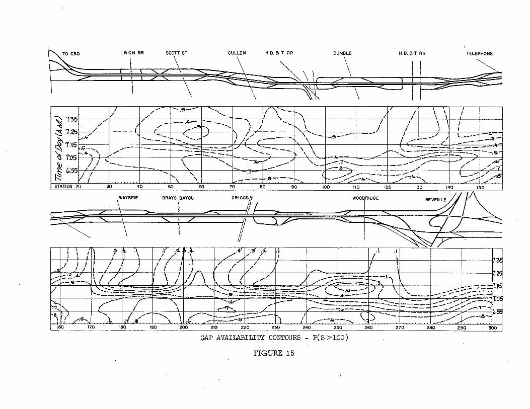
An appreciation of the effect of shoulder lane distribution on ramp capacity can be gained by determining the probability of securing a gap (space headway) of 100 feet or more .. This relationship is summarized for the Gulf Freeway study area in the form of probability contours (Figure 15 ) • The figure illustrates gap availability on the shoulder lane at a cer­tain location and time. A probability of • 25 means that on the average 1 gap in 4 is greater than 100 feet. For entrance ramps with gap acceptance re­quirements of 100 feete Figure 15 provides a dynamic description of accept­able gap availability. The ramp capacity is given by

( 35 )

with the constraint that

( 36 )

where q is the possible capacity of the shoulder lane. From equations 26 and f7 o it is apparent that equation 35 may be written

( 37 )

Thus u the parameter- E (n), in addition to being a theoretical device for describing congestion actually provides a rational means for operating exis­ting ramps and evaluating the capacity of future ramps.

-43-

1.8 G.N. RR SCOTT ST. CULLEN H.B. 8 T. RR

~\\ ~

DUMBLE H.B.ST.RR

' I

TELEPHONE

I ..- .._ .s--- '"-..._ /'\ .....__ -. 17 1 \ \ r I/ ,/ ......__ \. '\ I ; \ '

~ ~::,st /'I /l/ - ---""' ,...____ , ........... r-. \ ;; I ) ~ f ~ f . / ( ,/ .............. ?> -'\ ' 1 / ' .... .

~ 1:25 ,. ' -- <...._ / J /~,. --- \ -- --.s-- -- I! - f- _ _../ J l---1-_;:;_, '- ._.,.i<i ....__ -1--. _ _.. I // _("-- \ - /' ----r· !S' 1't5 .._ \ r-· :-:: --,- . ~ · 5--.. ....--- --- ,__:::::::-:=..::-F" __ :.::: ./ ~,....._ ----- \ --, '-- - .::::::-- ::-..:... __ -, --.s-'

,..,: ..... 4- '\ v,.,. -=:::.--- ., -- ' ,....._,., ., -- --r-· ..... i ~ 7:05 'J I , t , -~-,.,~ _., , -- _.:.-_.., __ - ....... - __ ..,...- /- ·-.. _,.,./,.,., J~ 1\, / -- ' ' - ,_ -- ~ ----- - .' ,.,.,.-;r !U • ~· / -~---- ' 1- - _. '.15- _,.., _,-

~ b.55 I I ...... . "- _,- . <. _.,.,.--'..,...1----- .... ---::..fo t-. \ - ...... ,.,/ ,.d5 ~ I/ 1 . .. . . . .. . . .. . . .. ....... ~\. ..... ~-I ......... ~..:.:-:-.=-"~::f-:·~.-.-:-:-:-:--:--:-,..., ...... ~--:':-:"' .-.-::"" ...... ':"~.~-:--:..- · .... -.~.... .":-. · · .. · · · -~-' · ./.. STATION 20 30 40 50 60 70 80 90 100 110 120 130 140 150

-....._ ""

dAYSIDE

\ BRAYS i""" ~ "'7t "> < -c7 WOT"" "" RE~ ~ ~ t 7 1 \ J g.... -..... -- -::s:.: -LJZ

1 ~/r"-~ I} ·', .\ :i· -~ .+ _ _...c.: .3 ,.,. .t :r- .I

j 1 / '. /,.//I I I l-./ I I I! I 1 I I I I I// /' / I I lor:~ n il', J I I

-~ :,.....' -

•• '2 ' I I I ; I j I ( I . j - i I_,/ / ,.,.,._ I ~or. v-:·::::')) -~ \ 1 / 1 ,.,..../ 1: \ 'Lil I \.\ 1 1 ,..../' v _______ t-----,l-,. :2~ 1/' 1---.s--.., \ l i ,. i I ./ r, \ ' / _,} ,./ ,.--:- ~.:;:;; -:3 \ ~/ \ '-.:::.."'::::."'::::.:" ____ _._Ff:-~ v '...., _ .............. :::::_- ---==--=-=. -=..::..:.:::..1--_,.., r "'r- s---",J I \ \ - ~-- ._:T:JS,

~~~ r:\Jr/

160

.r:s .....

- ~~---J;:_;-__.,..- -~ -----=---"' ' . _ ..... ( ... ~ ----- -------r:;:;;.---~ -- .-....-------=-- -- -, -- 4---- "~ ~ ~--- f.-• - ·-- - . '" ~ ---- 1'0~

170

_..,.,. t"' -...., -..,v --_.j -- ..... _ f-· -1-- ,_ - - - .....- -~ - ·- .. I' ........ ---t--- -----------/ ~........ ~ i \ ~~-r-.. / I/--- "' ------ ------- ..,..- ....- -.-r--. ' I ,.,...-r-...._ \ ....... --.......... -- - - I ' . - ........ - -::; ,...,.,., _, ":~ )._ / ..._ / -----'5' --- "\ I - l "\ - ------- ,..........- -~&-

• ._:r. ~·. . \. .. \ '~ ... -~ ."7":7-:-":. •. .. .. . .J ...... 1. . ./.----: .. ·~:- -:-:-~ ... > -:-.. .. .. . . .. .. .. . ___ ...... ./ 180 190 200 210 220 230 240 250 260 270 280 290 300

GAP AVAILABILITY CONTOURS - P(S >-100)

FIGURE 15

CONCLUSIONS AND RECOMMENDATIONS

Conclusions

The primary characteristics of traffic movement are concerned with speed, density and volume. Additional characteristics, associated with the traffic stream .. are the transverse and longitudinal distribution of vehicles. Interest in these characteristics is manifest in the need, and announced objective of this study to investigate those variables related to freeway congestion which can be determined and treated by surveillance equipment.

The stochastic aspects of the freeway traffic phenomenon were based on describing the longitudinal distribution of traffic mathematically.. The ErlanQI frequency distribution was utilized to describe the distribution of individual vehicles .. and a "moving queues" model was formulated to explain the tenden­cy of vehicles to platoon£ Applications of the stochastic approach to .traffic operations, freeway surveillance., and geometric evaluation and design are suggested~

The following conclusions are drawn regarding the announced objectives of this investigation ..

1~ The tendency of vehicles to form platoons provides a measure of the efficiency of a facility.$ The "moving queue" model, derived, is analogous to classical queueing in that the expected queue length provides a rational, quantitative index of congestion;

2. A comparison of the congestion predicting attributes of the three control parameters--optimum speed, optimum density and critical queue length--yielded close agreement in defining the time of incipient congestion throughout the length of the Gulf Freeway.

3 .. The moving queue parameter developed is capable of automatic detection~" measurement and control~

4 .. Since the moving queue length, E (n), was formulated in such a way that it is the reciprocal of the probability of receiving a gap larger than the queueing criteria 1 it is actually a measure of gap availability. This property makes it extremely important as a tool in rational geometric design and freeway capacity-design analyses.

The following additional conclusions are drawn regarding the data presented in this report.

1. The employment of time-lapse aerial photographic methods to measure such over-all operational characteristics as speed and density, and such local properties as acceleration, relative speed 1

-45-

and headways, is feasible~

2.. "Contour maps" provide an excellent means of illustrating variations in traffic characteristics in both time and space.

3~ By plotting the control parameters on the contour maps 1 it is apparent that approximately sixty percent of the Gulf Freeway operates above the critical queue length at some time during the morning peak hour.

4 .. The transverse distribution of traffic 9 evaluated both as to .lane occupancy (density) and lane usage (flow) over 7 00-foot: sections along the entire freeway r indicates inefficient use of the shoulder lane. This is caused by the drivers n tendency to avoid the shoulder lane in the vicinity of entrance ramps.

5., There does not seem to be any transverse pattern of failure prompted by the spread of congestion from one lane to another. As suggested above 1 drivers seem to compensate for turbulence in the shoulder lane,

6'"' There does exist a longitudinal hierarchy of operational fa.ilure .. Congestion sets in at various points on the facility and spreads to surrounding areas.

7,. The natural distribution of vehicles in the shoulder lane can be represented by the Erlang frequency distribution, based on 134 Chi Square tests ..

8. The longitudinal distribution of headways cannot be described by a single Erlang coefficient of randomness., The distribution varies in both time and space~ During conditions of free flow, the exponential distribution (a special case of the Erlang distribution) provides a satisfactory fit.. As congestion sets in 1 the distribution tends to change from randomness toward uniformity.,

9e The moving queue length equation provides a rational relationship between E (n) and k (density)., if distance is used as the queue cri­teria.

10., Because of the arbitrary nature of the queue criteria 1 the results can be extended to time headways, thereby relating E (n) and q (flow).

-46-

Recommendations

The control parameters established in this research provide a basis for the formulation of a rational "Level of Service 11 Index. Level oLService 1 as applied to traffic operation on a particular roadway o refers to the quality' of the dr:iving conditions afforded a motorist. In addition. to the variables designated as con­trol parameters, factors involved are: (1) travel time, (2) traffic interruption 1

(3) freedom to maneuver I {4) safety, (5) driving. comfontand convenlence,, and (6) vehicular operational costs. Additional research is needed to extablish a quantitative measure of these qualitative level of service factors, as a means of adjusting the control parameters in much the same manner that safety factors are utilized in structural design.

Regarding the results of this investigation 1 it is recommended that the moving queue parameter, E (n) 1 should be adopted as one basis for defining congestion 1 predicting congestion, controlling congestion and reducing con­gestion on new freeways at the design leveL

The expected number of vehicles per moving queue 1 E (n) 1 provides a quantitative index of congestion. This parameter may be oriented either to space headways or time headways. lt affords an index of congestion superior to volume if time headways are considered, or to density if space headways are considered, because E (n) takes into account the distribution of volume and density.

Similarly 1 the length of queue E (n) provides a quantitative means of evalu­ating freeway controls. The maximization of freeway output has been suggested as a figure of merit to be used as a guide in the operation of a freeway control system. If concessions are to be made to ramp traffic, who are also entitled to a reasonable travel time 1 perhaps "optimization" should be used instead of the word "maximization" to describe the desired objective of freeway operation.

The congestion index E (n) developed offers more than a subjective means of evaluating freeway performance. An automatic control system 1 based on moving queues 1 would have many advantages. The control system pictured in Figure 45 is simpler than a typical semi-actuated signal system at an intersection. The parameter E (n) is sensitive and therefore ramp traffic need not be unduly penalized when gaps in the outside freeway lane are available. The system could easily be expanded if more sophistication is desired. That is, a speed detector could be incorporated with the vehicle detector thereby adjusting Tp when speeds were reduced during the peak period. Moreover 1

several local controllers could be operated from a large computer 1 reducing

-47-

the possibility of undetected congestion due to shock waves.

The field of freeway traffic control offers both an opportunity and a chal­lenge to a multitude of manufacturers already engaged in traffic control .. or with capabilittties in this area. It is hoped that this model system wiil ; encourage more activity in the development of simple, rational( theoretically oriented hardware to control our freeways.

-48-

APPENDICES

-49-

APPENDIX A

SUMMARY OF OBSERVED DISTRIBUT.ION OF SPACE HEADWAYS (LANE 1) (10 feet interval)

PHOTOS 20 30 4o 50 6o ?0 80 90 100 110 120 130 140 >:1:5-o

ST~IP 1

8,10,13 18 25 23 17 6 4 3 1 1' 1 0 0 0 2 14,17,20 9 11 15 10 5 7 2 0 1 3 0 0 0 2 21,24,27 2 11 5 5 7 2 4 1 2 3 1 1 0 2 28,31,34 2 4 4 6 8 3 3 1 4 0 1 0 0 5 35,38,41 0 1 1 3 4 4 2 2 1 2 1 0 1 ()

42,4,5,48 0 1 3 4 4 3 2 1 2 4 0 0 1 4 49,52,55 0 1 1 0 0 2 3 0 3 2 0 0 0 4

I STRIP 3 01 0 I 115,118,121 11 23 22 14 12 9 2 1 0 0 0 0 0 l

122,125,128 8 12 11 9 8 7 1 1 1 1 0 2 0 3 129,132,135 5 9 10 6 5 4 6 2 2 0 2 0 0 3 136,139,144 3 5 9 7 3 4 1 ·1 4 0 1 1 1 5 143,146,149 0 0 3 4 3 4 0 0 ·1 0 1 1 0 7 150 '153' 156 0 0 3 3 4 3 1 .1 ~ 0 2 l 1 6

STRIP 4

6' 9', 12 '15 0 0 2 1 0 0 2 1 0 0 1 0 0 11 16,19,2'2 1 0 0 ' 0 1 2 2 'l :t l 0 0 6 23,26,29 0 0 0 2 0 0 1 2 1 ' 0 0 0 6 30,33,36 0 1 3 ·2 3 1 1 1 0 0 1 1 0 ? 37,40,43,46 0 0 1 i 0 2 0 0 3 2 1 2 2 10

SUMMARY OF OBSERVED DIST~.IBUTION OF SPACE HEABWAYS ('LANE 1) (10 Feet Interval)

PRO";[' OS 20 30 4o 50 60 70 80 !• l.OD .. 110 120 130 140 >150

STRIP '

116,119,1~2 1 0 1 0 4 0 4 0 2 2 1 1 1 10 123' 126' 12.9 () 1 1 4 2 2 0 3 1 2 4 1 1 6 130,133,136 0 0 1 a 2 0 2 4 1 3. 4 2 1 8 137,140,143 0 0 3 ~ 0 1 1 1 1 2 0 0 2 10

S.TR"IP 7

6,9,12 3 ' .10 6 .5 3 2 4 5 1 2 0 0 ' 13,16,19 1 0 1 1 ·2 3 0 0 2 4 1 3 0 7 20,2),26 0 2 2 0 1 2 3 1 4 3 1. 0 1 5

i 27,3<;),)'3 0 0 2 0 2 1 3 0 0 1 1 2 2 6 U1 34,37,40 0 0 0 3 1 1 2 2 1 2 0 1 1 6 ..... i 41,44,47 0 1 3 6 3 ~ 0 1 1 1 0 2 1 7

STRIP 9

97,lOO,i03 ? 1 9 2 9 8 9 3 1 1 1 0 0 2 104,107,1.10 5 .5 8 9 6 3 6 4 2" 0 2 1 1 3 11:1,114,117 l ~0 '( 10 8 4 3 2 2 2 3 0 2 6 118,121,124 0 2 4 4 .5 3 4 5 9 2 0 0 1 6 125,138,131 0 ~ 0 2 1 l 3 5 5 3 1 0 3 8 132' 135., 138 3 0 1 3 1 6 4 1 1. 0 3 1 1 7

APPENP!X 12

OBSERVED QUEUE LENG'ffl MEASUREMENTS (LANE 1)

STRIP 1 STRIP 3 STlUP 4 STRJ:·p 6 STRIP 7 STRIP 9 PHOTO E(n) PHOTO E(n) PH01'P E(n) PHOTO E(n) PHOTO E(n) PHOTO E (n·)

7 47.0 114 3.0 6 1.0 115 1.0 6 2.2 95 7.0 8 48.0 11.5 1.5 • .5 7 l.Q 6 1.1 7 2.0 6 3.5.0 9 44.o 116 41.0 8 l.Q ? 1 .,4 8 2.3 7 34.o ·

10 42 .. 0 11? 4').0 9 1.~~ 8 1.3 9 4.o 8 4o.o 1,1 37.0 118 4o.o 10 1 .. :} 9 2.0 10 ?eO 9 44;,0 12 1?.,0 119 3.5 .o 1 1 .. ~ 120 1 • .5 1 3 .. 4 100 43.0 13 ?.3 120 15 •. 5 2 2 .. 'J 1 1.,.2 2 1 .. 9 1 1.5 •. o 14 10.,7 121 35 .o 3 1.1,5 2 1.6 3 2 • .5 2 4.8 1.5 11.0 122 37 .. 0 4 1.~ 3 1.9 4 2.3 3 2 •. .5 16 6.5 123 45 .o 1.$ 1.9 4 2.0 5 2.0 4 2.3 1? a.o 124 21e.5 6 1.3 12.5 2.0 6 1.6 5 5 •. 5 18 33.0 12.5 19 .. 5 ? i:·j 6 2e0 7 1.3 6 10.0 19 11.3 126 7 .. 0 8 7 1 • .5 8 1 o.6 7 17.5 20 9·7 12'7 8., . .5 9 2.j e 1.4 9 la7 8 11.3 21 6.3 128 3.2 20 2 .. 4 9 J..5 20 2.,0 9 4.o 22 3.2 129 2.4 1 l.J.t, 130 )..,'J 1 1.6 110 3 •. 2 23 2 .. 6 130 2.0 2 i:l 1 1.4 2 1.2 1 2.1 24 3.3 131 3 .. 9 3 2 1., 3 1.3 2 2,.5 2:.5 6.3 132 12.0 4 q 3 1.9 4 1.6 3 4 • .5 2:6 17.0 133 6.o 2.5 4 1.,7 5 1.J 4 17.0 27 4 •. 8 t34 4.8 6 13.5 1.4 6 le~7 5 30 •. o 28 3e,3 135 4 ... 2 7 2.' 6 1 •. 2 7 1.9 6 3 •. 6 29 2.0 136 ?.7 8 1 .. 1~ 7 1.2 8 2.0 7 2.1 30 4.8 137 ?.3 9 1. 8 1.4 9 1.? 8 2.4 31 4 • .5 138 10.3 30 2 .. ~ 9 lo4 30 1 .. 4 9 2.7 32 ?.0 139 4,.? 1 2.~ 140 1 .. ? 1 1.,7 120 4.8 33 6.3 140 2.7 2 2.$ 1 2.7 2 1.7 1 6.0 34 3.0 141 1 .. 9 3 3·! 2 1 .. 3 3 1.9 2 3 •. o 35 2.8 142 2.4 4 2 .. 0 3 1.2.5 4 1.8 3 2 ... .5 36 3.0 143 1.9 3.5 1 .. 9 4 1 .. 2 5 2.1 4 1.8 37 3.,0 144 1.6 6 1 .. 7 145 1.7.5 6 2.0 5 1.7 38 3.2 14.5 2.3 7 1.? 6 1.4 7 1 • .5 .6 i.S 39 3 .. 2 146 3.2 8 ;t.8 8 1.7 7 1.4 4o 2.,1 147 2e9 9 1.1 9 2.2 8 1.6 41 1.8 148 2.8 4o 1 .. 0 4o 1.9 9 1.3 42 1.4 149 1•8 i 1.0 1 1 .. 3 130 1.5 43 1.4 l.50 t.3 2 leQ 2 1.1 1 1.8 44 1.8 1.51 1.7 3 l.Q 3 1.3 2 2.3 4,5 2.1 ;1.52 2.3 4 1 .. 3 4 1.2 3 2.,? 46 3 .. 8 1.53 3.0 45 1 .. ~ 5 2.,3 4 2 .,7 47 4.! ;t54 2.8 6 1.3 6 2.3 5 2.0 48 5 .. 3 1.55 2.8 7 1.6 7 3.2 6 1 •. 7 49 2 .. 6 1.56 2.0 8 1.8 7 2.-.5 50 2 •. 7 1.57 1.4 8 2.8 51 2.3 158 1.3 9 4.o 52 2.0 1.59 1.3 140 2.3 53 2.0 160

-52-

BIBLIOGRAPBY

1~ Gerlough~- D., Lq "Traffic Inputs for Simulation on a Digital Computer~-~~ Proceedings of Highway Research Board, Vol~ 38, 1959 1 pp .. 480-492,

2., Schuh!, Andre, " The Probability Theory Applied to the Distribution of Vehicles on Two-Lane Highways, " Poisson and Traffic , The Eno Founda­tion ( 1955 ),

3, Haight 1 Frank A. 1 Mathematical Theories of Traffic Flow 1 Academic Press 1 New York 1 1963.,

4, Miller 1 A. J_.., "Traffic Flow Treated as a Stochastic Process," Theory of Traffic Flow., Elsevier Publishing Company, New York, 1961.

5, Keeseu C. J., Pinnell1 Charles, McCasland, W. R., "A Study of Free­way "Traffic Operation," Highway Research Board, Bulletin 235~

6. Lipscomb r J .. N"' 6 II The Effects of Ramps on the Lateral Distribution of Vehicles on a Six Lane Freeway. 11 Thesis 1962, Texas A&M University.

7., Ginn, J $ R. 1 " Peaking Characteristics on Urban Freeways i" Unpublished.,

8., McCasland .. W. R. 1 11 Comparison of Two Techniques of Aerial Photographs

for Application in Freeway Traffic Operations Studies," Presented at 43rd Annual Meeting of the Highway Research Board, 1964 1 Washington1 D~ C.

9.. Foote.e R. S, rr Crowley, K., W" g and Gonseth, A. T., "Development of Traffic Surveillance Systems at the Port of New York Authority .. "

10. May, A~ D .. r Atholr P,,. Parker 1 W ... , and Ruddenr J. B.,, "Development and Evaluation of Congress Street Expressway Pilot Detection System., " Highway Research Boardu Record No., 2 L.

1 L Drew.~ Donald R • ., "Deterministic Aspects of Freeway Operations and Control.," Texas Transportation Report, Texas A&M University<>

12" Pinnell, Charles, and Keese., C., J .,_,. "Freeway Ramps," Texas Trans­portation Institute Report, Texas A&M University &

-53-

PUBLICATIONS

Project 2-8-61-24 Freeway Surveillance and Control

1. Research Report 24--1., "Theoretical Approaches to the Study and Control of Freeway Congestion~' by Donald R., Drew.

2 o Research Report 24-2, "Optimum Distribution of Traffic Over a Capacitc;rted Street Network" by Charles Pinnell.

3. Research Report 24-3, "Freeway Level of Service as Influenced by Volume Capacity Characteristics" :by Donald R., Drew and Charles J. Kees.e.

4., Research Report 24-4, "Deterministic Aspects of Freeway Oper­ations and Control" by Donald R,~ Drew,.