Stochastic Analysis of Long-Term Multiple-Decrement Contracts

© 2008 Society of Actuaries

Stochastic Analysis of Long-Term Multiple-Decrement Contracts

Matthew Clark, FSA, MAAA, and Chad Runchey, FSA, MAAA Ernst & Young LLP

Published in the July 2008 issue of the Actuarial Practice Forum

Copyright 2008 by the Society of Actuaries. All rights reserved by the Society of Actuaries. Permission is granted to make brief excerpts for a published review. Permission is also granted to make limited numbers of copies of items in this monograph for personal, internal, classroom or other instructional use, on condition that the foregoing copyright notice is used so as to give reasonable notice of the Society's copyright. This consent for free limited copying without prior consent of the Society does not extend to making copies for general distribution, for advertising or promotional purposes, for inclusion in new collective works or for resale.

2 © 2008 Society of Actuaries

Table of Contents Executive Summary ......................................................................................3 Introduction..................................................................................................6

Product Selection ........................................................................................................... 6 Deterministic Results...................................................................................................... 7 Stochastic Decrements .................................................................................................... 8

Stochastic Mortality ......................................................................................9 Introduction to Stochastic Mortality ................................................................................. 9 Stochastic Mortality Factors ............................................................................................ 9 Stochastic Mortality Generator ...................................................................................... 10 Stochastic Mortality Results .......................................................................................... 12 Sensitivity Analysis...................................................................................................... 15 Summary..................................................................................................................... 16

Stochastic Lapse .........................................................................................17 Introduction to Stochastic Lapse .................................................................................... 17 Stochastic Lapse Generator ........................................................................................... 17 Stochastic Lapse Impact on Mortality............................................................................. 18

Stochastic Lapse and Mortality ...................................................................20 Reinsurance ................................................................................................21

Introduction of Reinsurance .......................................................................................... 21 Excess Reinsurance ...................................................................................................... 21 Experience Refund ....................................................................................................... 24 Multi-Year Stop Loss ................................................................................................... 26 Reinsurance Summary .................................................................................................. 27

Supplemental Insights .................................................................................30 Summary ....................................................................................................30 Attachment A: 20-Year Term Insurance Assumptions.................................32 Attachment B: 20-Year Term In Force Summary........................................34 Attachment C: Stochastic Lapse Impact on Mortality .................................36 Attachment D: Stochastic Decrements Literature Review ............................38


Executive Summary As risk management matures in the insurance industry, the universe of risks measured will continue to expand, and modeling techniques will continue to advance. Stochastic modeling techniques have captured the interest of the insurance arena. As insurance products have evolved to include options and guarantees, traditional deterministic regulatory and risk measurement techniques have proven to be inadequate to fully understand the risk profile of an organization. Deterministic valuation techniques provide a limited view of the risk profile of a product or organization. Although the introduction of stochastic modeling techniques has aided the insurance industry in the quantification of market risks including low-incidence, high-severity tail events, the industry has continued to value nonmarket risks using traditional valuation techniques. This report is sponsored by the Society of Actuaries in collaboration with Ernst & Young. It examines the application of stochastic modeling techniques to nonmarket risks facing the life insurance industry. The focus of this paper is the modeling and quantification of mortality and lapse risks with consideration for the impact reinsurance has on these risks. To mitigate the impact of financial risks, the research assumes a 20-year term life insurance product. This report is intended to be a resource document for actuaries, risk managers, and other interested parties. This project also includes a literature review of stochastic decrement modeling found in Attachment D. Traditionally the valuation of insurance risks has been performed using deterministic techniques with limited sensitivity analysis. Alternatively, stochastic analysis focuses on the generation of a universe of potential events over which the liability cash flows are generated. Once generated, this universe of events provides a risk profile of the policyholder options, guarantees, and decrements. Stochastic analysis introduces the need to create and calibrate scenario generators. Borrowing from the techniques employed with market risks and a careful understanding of the risk composition of mortality and lapse behavior, stochastic generators can be created to reflect the nonmarket risks faced by insurance companies. The parameterization of these generators needs to be performed with consideration of the current and evolving risk profile of the organization. Balancing historic events with the risk universe is important when focusing on the tail of the risk distribution. To create a mortality scenario generator, it is essential to understand the origin of the risks inherent in mortality. In short, mortality risk is composed of four risk elements, including error generated in the underwriting process, volatility around the best estimate, catastrophic events that impact mortality, and the trend in mortality (improvement or deterioration). When stochastically


modeled, the relative contribution and risk profile of each risk element can be evaluated. It is important to understand how each risk element contributes and interacts to create the cumulative risk profile. A critical step in the process is the evaluation of the stochastic results not only to gain an understanding of the risk profile but also to also understand the impact parameterization of the stochastic generator has on the results. Generating stochastic mortality results provides a distribution of results that an organization faces and the severity and incidence of the tail events. The relative contribution and interaction of the individual mortality risks provide insight into the risk profile. Like mortality risk, the deterministic lapse assumption used in the best estimate projection of liability cash flows reflects the lapse activity that a life insurance company would expect on average. For the term insurance product modeled, the lapse function was not directly tied to the market or any other observable factors. The lapse risk was modeled to reflect the volatility around the best estimate. The derivation and parameterization of the stochastic lapse generator used for this report are similar to those used for mortality risks with the exception of the individual risk elements for underwriting, catastrophe, and trend. Unlike mortality risk, lapse behavior is at the discretion of the policyholder, resulting in a significantly higher volatility parameter. Generating stochastic policyholder lapse activity also requires consideration of the impact lapse activity has on the mortality of the remaining insured population. Policyholders that elect to lapse their life insurance coverage on average display lower mortality risk than policyholders that are generally poorer risks that elect to persist their insurance coverage. Modeling the impact of increased mortality due to increased lapse activity requires careful consideration of the population demographics and the evolution of the underlying mortality risk. Generating the stochastic mortality and lapse experience in isolation provides independent risk profiles. When these risks are integrated, the combined risk profile illustrates the correlation of these risks at all points of the distribution. With the exception of the deterioration of the insured population mortality related to excess lapse activity, the incidence of variance in lapse and mortality are assumed to be independent. This independence results in a combined risk profile that displays less volatility than the arithmetic sum of the individual risk events. In short, tail mortality events do not necessarily occur at the same time as tail lapse events. Reinsurance is a common medium used by insurance companies to limit their exposure to mortality risk. Integrating reinsurance agreements with a stochastic mortality model provides insight into the net impact reinsurance has on the risk profile of an insurance portfolio. On a deterministic basis, the introduction of reinsurance reduces the capital position of an organization by an amount near the cost of the reinsurance coverage. In short, reinsurance agreements generally provide coverage for tail events that are not captured in best estimate projections. Expanding the analysis to include the stochastic mortality scenarios provides a distribution of events to better understand the impact reinsurance has on the overall risk profile. The net impact


of reinsurance reduces the volatility of the mortality risk events resulting in less capital required to fund tail mortality events. The characteristics of each reinsurance agreement have a unique impact on the net capital requirement. Some reinsurance agreements are intended to reduce extreme tail events while other agreements provide a lower overall exposure to mortality. As product complexity increases and insurance companies are looking to better understand the entire risk profile of the organization, the modeling of stochastic decrements is going to become an important step in the process. The research performed for this report uncovered several areas where additional research is needed, including the following:

• Analyzing the impact of different probability distributions for mortality and lapse analysis

• Examining the impact of different parameters for the stochastic mortality and lapse generators

• Using more robust modeling of stochastic lapses, including interaction with economic and market variables

• Generating stochastic results under various accounting frameworks (i.e., considering the assumptions underlying GAAP earnings over a range of stochastic events)

• Incorporating stochastic decrement modeling with other products and examining the interaction of market, credit, mortality and lapse risks.

In summary, stochastic analysis is a tool that actuaries can use to better understand the impact nonmarket risks have on a product or enterprise. Many different issues need to be addressed, including, but not limited to, the underlying probability distribution, parameterization and interaction of risks. The information generated is invaluable in understanding the risk profile and providing the tools needed to better manage a company’s exposure to all risks, including mortality and lapse risks.


Introduction Traditional actuarial modeling has been based on deterministic scenarios using best estimate assumptions. From a regulatory perspective, the valuation of insurance liabilities has been formulaic with conservatism added to select assumptions to provide the desired margins. The use of deterministic scenarios has served the insurance industry well in the past, and some simple scenario analysis has been performed. Cash flow testing is an example in which multiple scenarios have been integrated into the valuation of insurance liabilities. The standard scenarios included in cash flow testing were derived to test the adequacy of reserves with a desired tail sensitivity related to interest rate risks. Advances in product development and technology have led to the need to pursue a more robust solution. That solution is the introduction of stochastic modeling. Stochastic modeling is not new to the valuation of financial options and guarantees. The financial market has moved from closed-form valuation to stochastic processes. These techniques have migrated to the insurance market and can be seen in the valuation and pricing functions at most companies. The introduction of C3 Phase II capital requirements for variable annuities is an example in which regulators have introduced stochastic analysis. Stochastic valuation provides a process where the cash flows of an insurance liability are generated over a universe of outcomes. Without stochastic processes, the valuation of guarantees and options would be left to closed-form solutions and deterministic scenarios. These closed-form solutions are often extremely tedious and difficult, if not impossible, to derive. Deterministic scenarios do not allow an organization to create a full distribution of the potential outcomes. In short, deterministic valuation provides a limited view of the risk profile of a product or organization. The introduction of stochastic processes brings with it several considerations. Two of the issues that the user must address are (1) the calibration of the scenario generator and (2) the run time required to run the new universe of scenarios. These challenges and how they were addressed for this project will be covered later in this paper.

Product Selection To focus the analysis on stochastic policyholder decrements, a product was selected that provided exposure to policyholder decrements while minimizing the exposure to other risk elements. The selection of the level face amount term life insurance product provided the exposure to mortality and lapse activity desired, as well as simplicity around the modeling and communication of results. The assets backing term business are relatively small, and therefore


the investment returns are not a primary driver of financial performance. The primary risk drivers for this product are mortality and lapse experience. Attachment A summarizes the modeling assumptions used to price and model the level term business. Although the assumptions were selected in an effort to reflect realistic conditions, the focus of this project was on the impact that stochastic decrements have on the financial performance of an insurance company. An in-force population was generated using pricing assumptions, reflecting level sales of 1,000 policies a year over the prior 21 years with a midyear valuation assumed. The in force is distributed across three issue ages (35, 45, and 55) and three face amounts ($250,000, $1 million, and $5 million). It is assumed that all individuals start in the same underwriting risk category. The in force was derived assuming an equal number of policies issued to each of the nine cohorts (defined by issue age and face amount). All of the policies were assumed to be male for simplicity. No future sales were included in the model. A summary of the population demographics can be found in Attachment B. In the model the assets are assumed to earn a level rate of return of 5.50 percent over the duration of the projection. The liability assumptions were set to generate an internal rate of return approximately equal to 14 percent over the level term period.

The liability assumptions were calibrated to reflect a product with realistic cash flows. Where decisions needed to be made with respect to assumptions and methodology, the modeling effort and intent of the study were the driving forces.

Deterministic Results Although the pricing and assumption calibration exercise was completed using statutory cash flows, it was decided to reflect the results of the project using what will be referred to as a “cash balance” approach. The focal point of the exercise was to understand the change in cash flows generated by the introduction of stochastic decrements. The selection of the cash balance method was made because it captures the cash flows that occur without the complications that accounting can introduce. Below is a summary of the cash flows that are included in the calculation as well as the net impact positive or minus from the company perspective:

Premiums (+) Premium Tax (−) Death Benefits (−) Expenses (−) Commissions (−) Investment Income (+)


The asset balance at time zero is set equal to the statutory reserves for the in-force population. The cash flows are accumulated throughout the projection period, 30 years from today, to arrive at an ending asset balance. Asset balances were discounted using the assumed earned rate of 5.50 percent. Table 1 contains a summary of the initial balances and the results for the deterministic scenario.

Table 1 Deterministic Run Results

Face amount $22,575,994,568 Initial assets 628,487,113 Present value of ending assets 449,968,162

Because the discount rate was the same as the earned rate, the difference between the present value of ending assets and initial assets represents the present value of future cash flows. In the deterministic example, the present value of future cash flows is approximately −$179 million ($450 million ending assets less $628 million initial assets). The level premium nature of the term product selected explains the negative net cash flow where early premiums in excess of expected mortality fund death claims in the later years. The remainder of this report will reference this deterministic result as a point of comparison for future scenarios to evaluate the relative impact of each analysis on the future cash flows expected by the company.

Stochastic Decrements Stochastic modeling in the insurance industry has historically been focused on the financial risks faced by insurance companies (e.g., interest rate, equity, and credit risks). The development of stochastic modeling for nonfinancial risks is a recent trend as insurance companies are recognizing the need to generate and understand their risk profile across all the risks facing the organization. Although numerous nonfinancial risks face insurance companies, this report focuses on the assumptions and analysis related to policyholder decrements, specifically mortality and lapse risks faced by life insurance companies. To model mortality and lapse risk, one must first understand the cause for variance in policyholder decrements. We will define a methodology to derive a set of stochastic scenarios to incorporate in the 20-year level term life insurance model. The parameterization and model structure will have a material impact on the results and findings made regarding the exposure to policyholder decrements. The application of the techniques outlined in this report is intended to be illustrative in nature. Practitioners will have to use care in the selection and parameterization of stochastic techniques. It is the goal of this report to provide insight and understanding into the impact stochastic techniques will have on the modeling of policyholder decrements.


The remainder of this report focuses on the impact modeling decrements using stochastic processes has on the cash flows of an insurance company.

Stochastic Mortality

Introduction to Stochastic Mortality To this point, a level term cash balance model has been established and the calculation of the ending asset balance on a best estimate deterministic basis has been performed. Best estimate analysis provides insight into the cash flows under a single scenario, assuming that the best estimate assumptions are correct. The reality is that the best estimate assumptions are subject to variances that limit the usefulness of this single scenario. The pricing and management of insurance liabilities include consideration for the risks faced under a variety of conditions. Insurance companies and financial institutions have integrated stochastic economic processes in which products are analyzed across numerous economic scenarios. These scenarios are generated using an economic scenario generator with parameters estimated using historic market experience, current market conditions, and user judgment. As indicated previously, the intent of this project is to gain insight into the impact policyholder decrements have on the results of a life insurance product, more specifically a 20-year level term product. Given the limited assets backing term business, the majority of the risk faced by an insurance company is generated by policyholder decrements (mortality and lapse). The first decrement that will be investigated is the policyholder mortality assumption. The deterministic mortality assumption used in the best estimate projection reflects the mortality that a life insurance company would expect on average. Mortality, like other risks, typically does not evolve consistent with expectations. In fact, the mortality assumption for a select demographic is not consistent over time as conditions such as medical advances and improvements in the quality of life occur. To understand the impact the deviation in mortality has on the profitability of a product, one must first understand the forces underlying the movement in mortality rates and derive a scenario generator to produce a set of scenarios.

Stochastic Mortality Factors The deviation in mortality experience can be attributed to four factors outlined below:

• Underwriting Error—A risk is present that the best estimate assumption is incorrect. The ability to reflect the expected mortality experience accurately is generally dependent on the underwriting process. The focus will not be on the source of underwriting risk, but on the fact that it exists.


• Volatility—As with other assumptions, the actual experience will vary around the central value defined as the best estimate. Mortality exhibits this same behavior with the volatility level dependent on the size of the population. As the population grows, the volatility decreases.

• Catastrophe—Populations are exposed to events that result in a sharp increase in mortality for a short period of time. These events would include pandemics, natural disasters, and terrorist attacks. The severity and frequency of catastrophic events are difficult to predict. The calibration of the catastrophe risk is a difficult task, because historic events may not be indicative of future conditions.

• Trend—As medical advancements occur and quality of life improves, the life expectancy increases across a population. Consistent with the catastrophe element, the calibration of the mortality trend is a difficult task because historic improvements may not be indicative of future improvement expectations. Note: This factor was excluded from this analysis because trend is not a critical component of the mortality risk that companies writing this product face. However, when looking at other insurance products, such as a payout annuity, trend is a critical component and should not be excluded.

Stochastic Mortality Generator Now that the mortality elements that should be reflected in the stochastic process have been defined, the next step is to generate a set of mortality scenarios. Several different approaches have been used to look at potential mortality experience that were not included in this paper. One of the alternate approaches is to perform a simulation on each of the lives in the cohort to determine the age at death. Another approach uses stochastic processes to generate a mortality rate for each period. For this analysis, a global mortality factor was selected to reflect the variance in mortality experience. In other words, the mortality generator creates a single factor to be applied against the base mortality rate for the entire population regardless of cohort. A single factor was generated for each projection year (30-year projection horizon) within each scenario. The term model was run under 10,000 stochastically generated mortality scenarios. The number of scenarios was selected as a compromise between run time and convergence of results. In the end, the stochastic mortality generator produces a 30 × 10,000 matrix of factors. The factors generated are the product of three separate factors, each representing one of the mortality factors defined above. A summary of the factors and underlying distributions is provided in Table 2.


Table 2

Stochastic Mortality Risk Element Distributions Stochastic Element Underlying Distribution Mean Standard Deviation Underwriting factor Lognormal 1.00 5% Annual mortality volatility Lognormal 1.00 5% Underlying Distribution Incident Probability Catastrophe shock Binomial 300% 1 in 100 year event

The first stochastic element is the underwriting factor. As defined above, the underwriting factor is generated to reflect errors in the underwriting process. Given that the best estimate assumption is the baseline expectation around which the volatility will occur, the mean factor is assumed to be 1.00. A lognormal distribution was selected to generate the mortality scenarios. The selection of the standard deviation was made to be indicative of industry practice. However, actual variance in mortality volatility is highly dependent on each company’s business. Users may calibrate the standard deviation to reflect the accuracy of their underwriting process. Using a random number generator, a set of 10,000 factors was generated to derive the underwriting factors. Note that a single underwriting factor was produced per scenario and applied to all cohorts. This implies that underwriting errors were not corrected with new sales and affected all issue years the same. Alternatively, a different underwriting factor could be used for each cohort. In this modeling the factor was applied for all projection periods. The application of a single factor by scenario is consistent with the theory that underwriting risk is consistent over the life of a cohort and does not change by year unless process changes are implemented. To combine all of the mortality risk factors, a 30 × 10,000 matrix of random numbers was generated. Note that the single factor by scenario is repeated across the 30 years for each of the 10,000 scenarios. The second stochastic mortality factor is the annual volatility of the mortality rates. As with other assumptions, the best estimate mortality reflects an average assumption over time. The actual mortality incidence will occur around the best estimate. The standard deviation around the best estimate is inversely related to the size of the population. As the population increases in size, the volatility around the best estimate mortality assumption decreases. A standard deviation assumption of 5 percent was used, which is consistent with the standard deviation currently employed by many large insurers. The random number generator was used to create a 30 × 10,000 matrix of random numbers. The third stochastic mortality factor is the catastrophe shock. Consistent with the volatility generator, we generated a 30 × 10,000 matrix of factors. For the selected distribution, each projection year is subject to a catastrophic event with a 1 percent probability and a mortality expectation of 300 percent of the best estimate assumption. The frequency and severity of the catastrophic events were selected to be consistent with historic events and meant to be illustrative. Many more complex stochastic generating techniques for catastrophe shock exist, as well as theories on how catastrophic events will impact future mortality at the cohort level. These theories focus on the demographic impact of select catastrophic events. The impact of an


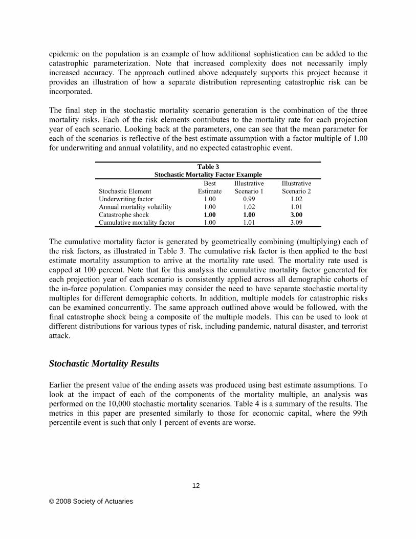
epidemic on the population is an example of how additional sophistication can be added to the catastrophic parameterization. Note that increased complexity does not necessarily imply increased accuracy. The approach outlined above adequately supports this project because it provides an illustration of how a separate distribution representing catastrophic risk can be incorporated. The final step in the stochastic mortality scenario generation is the combination of the three mortality risks. Each of the risk elements contributes to the mortality rate for each projection year of each scenario. Looking back at the parameters, one can see that the mean parameter for each of the scenarios is reflective of the best estimate assumption with a factor multiple of 1.00 for underwriting and annual volatility, and no expected catastrophic event.

Table 3 Stochastic Mortality Factor Example

Stochastic Element Best

Estimate Illustrative Scenario 1

Illustrative Scenario 2

Underwriting factor 1.00 0.99 1.02 Annual mortality volatility 1.00 1.02 1.01 Catastrophe shock 1.00 1.00 3.00 Cumulative mortality factor 1.00 1.01 3.09

The cumulative mortality factor is generated by geometrically combining (multiplying) each of the risk factors, as illustrated in Table 3. The cumulative risk factor is then applied to the best estimate mortality assumption to arrive at the mortality rate used. The mortality rate used is capped at 100 percent. Note that for this analysis the cumulative mortality factor generated for each projection year of each scenario is consistently applied across all demographic cohorts of the in-force population. Companies may consider the need to have separate stochastic mortality multiples for different demographic cohorts. In addition, multiple models for catastrophic risks can be examined concurrently. The same approach outlined above would be followed, with the final catastrophe shock being a composite of the multiple models. This can be used to look at different distributions for various types of risk, including pandemic, natural disaster, and terrorist attack.

Stochastic Mortality Results Earlier the present value of the ending assets was produced using best estimate assumptions. To look at the impact of each of the components of the mortality multiple, an analysis was performed on the 10,000 stochastic mortality scenarios. Table 4 is a summary of the results. The metrics in this paper are presented similarly to those for economic capital, where the 99th percentile event is such that only 1 percent of events are worse.


Table 4 Stochastic Mortality Impact by Risk Element

Metric Underwriting Annual Volatility Catastrophic Cumulative 99th percentile (160,168,290) (39,791,967) (264,370,773) (327,020,135) 95th percentile (116,202,897) (28,578,260) (199,383,175) (209,626,299) 90th percentile (88,522,044) (22,771,615) (125,799,822) (152,565,171) 75th percentile (45,036,396) (12,564,296) (5,732,206) (78,471,599) 50th percentile 812,377 (1,542,441) — (17,535,442) 25th percentile 46,664,475 9,366,531 — 35,149,357 10th percentile 85,163,501 19,190,323 — 77,956,593 5th percentile 108,839,976 25,003,882 — 101,812,488 1st percentile 154,489,059 35,370,942 — 151,652,389 Average (293,810) (1,711,943) (27,816,865) (29,822,618) Standard deviation 68,002,465 16,297,634 66,495,189 96,262,438

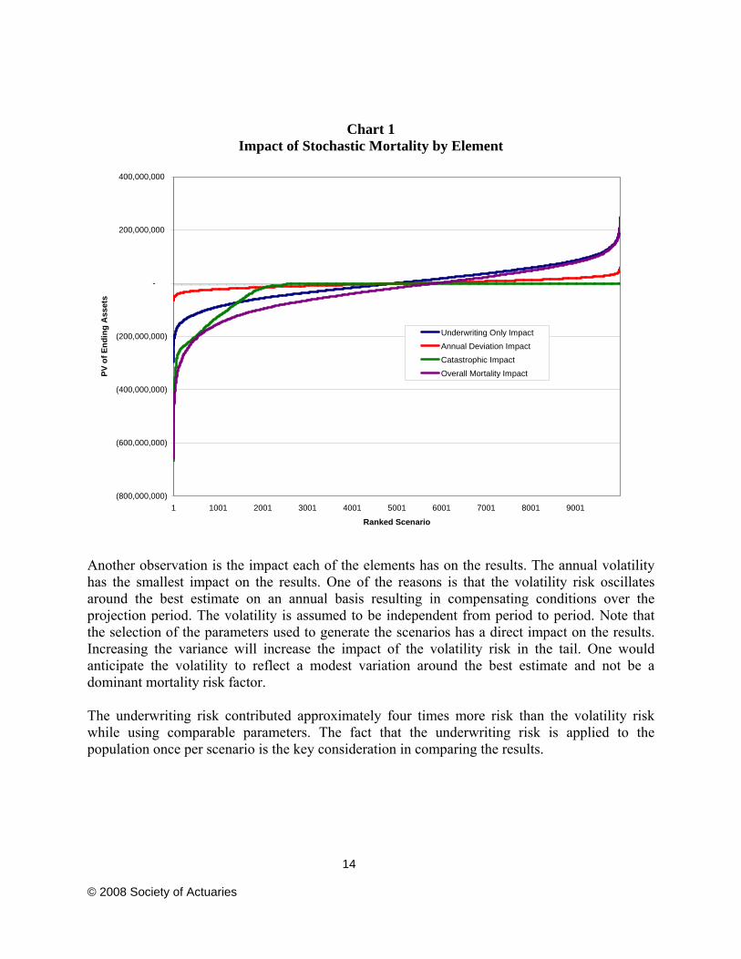
When the results for the best estimate scenario were generated, the present value of the ending asset balance was reported as $449,968,162. The results above are reported relative (difference between each scenario and the best estimate) to the best estimate scenario. For example, the impact of the underwriting component at the 99th percentile was a $160 million decrease in the present value of future cash flows. These results will be referred to as the “Delta” in future exhibits. The results for each risk element are ranked across the 10,000 scenarios from the best to the worst result. The cumulative result reflects the combination of the risk events as they were generated. The cumulative column is not generated as an addition across the individual risk events. In other words, the worst catastrophic event does not necessarily coincide with the worst underwriting event. This can be seen by looking at the 99th percentile results across each of the mortality risk elements. In the absolute value, the sum of the “Delta” values exceeds the cumulative entry. As designed in this analysis, the catastrophic event is a one-sided distribution. The risk incidence is a 1 in 100 year event that only impacts the mortality results when the event occurs. One might expect the results to reflect an event only in the far tail (99 percent) of the distribution. The actual results reflect an impact on results starting around the 75th percentile. The fact that the catastrophic event is an annual factor and the projection period was 30 years means that nearly 30 percent of the scenarios will include at least one catastrophe event during the projection. This can be seen in Chart 1, as the catastrophic mortality impact starts to be measurable at approximately the 3,000th scenario.


Chart 1 Impact of Stochastic Mortality by Element

(800,000,000)

(600,000,000)

(400,000,000)

(200,000,000)

-

200,000,000

400,000,000

1 1001 2001 3001 4001 5001 6001 7001 8001 9001

Ranked Scenario

PV o

f End

ing

Ass

ets

Underwriting Only ImpactAnnual Deviation ImpactCatastrophic ImpactOverall Mortality Impact

Another observation is the impact each of the elements has on the results. The annual volatility has the smallest impact on the results. One of the reasons is that the volatility risk oscillates around the best estimate on an annual basis resulting in compensating conditions over the projection period. The volatility is assumed to be independent from period to period. Note that the selection of the parameters used to generate the scenarios has a direct impact on the results. Increasing the variance will increase the impact of the volatility risk in the tail. One would anticipate the volatility to reflect a modest variation around the best estimate and not be a dominant mortality risk factor. The underwriting risk contributed approximately four times more risk than the volatility risk while using comparable parameters. The fact that the underwriting risk is applied to the population once per scenario is the key consideration in comparing the results.


The catastrophic risk creates the largest negative result. Using the scenarios we generated, the catastrophic events require the use of approximately $264 million more assets at the 99th percentile than the best estimate. As indicated above, the catastrophic events only result in a negative impact on the results.

Sensitivity Analysis It is important to perform sensitivity analysis when selecting the parameters used in the stochastic mortality generator. Below is a summary of the analysis performed and decision process employed in the selection of the catastrophic parameters used above. Some discussions regarding the catastrophic parameters center on the severity and length of a catastrophic event. Although it was decided to use a single-year exposure with a 300 percent mortality assumption, analysis was performed to understand how a 200 percent mortality event over three years would impact the results. This sensitivity was selected to change the characteristics of the catastrophic event to be less intense but last for a longer period of time. Many different types of events that could be modeled simultaneously using the approach outlined in the paper. The scenarios for underwriting error and annual volatility were not changed. Table 5 presents a summary of the results for the “cumulative” impact of all mortality elements for each catastrophic parameter sensitivity. Chart 2 shows the distribution of those results.

Table 5 “Delta” Results: Catastrophic Risk Sensitivity

Metric One-Year Catastrophic

Event of 300% Three-Year Catastrophic

Event of 200% 99th percentile (327,020,135) (420,997,843) 95th percentile (209,626,299) (272,975,261) 90th percentile (152,565,171) (188,126,244) 75th percentile (78,471,599) (84,962,192) 50th percentile (17,535,442) (19,464,659) 25th percentile 35,149,357 34,249,175 10th percentile 77,956,593 77,597,738 5th percentile 101,812,488 101,594,736 1st percentile 151,652,389 151,585,068 Average (29,822,618) (40,033,749) Standard deviation 96,262,438 113,090,210


Chart 2 Catastrophic Parameter Sensitivity

0

100

200

300

400

500

600

(450) (340) (240) (140) (40) 60 160 260

"Delta" - PV of Ending Assets (in Millions)

Num

ber o

f Sce

nario

s

300% - 1 Year 200% - 3 Years

The intent was to determine realistic parameters for a catastrophic event; the ultimate observation reflected the impact catastrophic events had on mortality. The sensitivity that was performed for this analysis did not significantly alter the distribution of results. However, using alternative distributions for the catastrophic mortality risk may result in different findings.

Summary The introduction of stochastically generated mortality scenarios has introduced volatility around the best estimate results. This volatility reflects the uncertainty that is observed over time around the risks facing mortality. Modeling mortality risk using a deterministic scenario does not reflect the full profile of the risk. The stochastically generated results illustrate the distribution of results that an organization faces, and the severity and incidence of the tail events are important to the management of the risks faced by an organization. Later, the introduction of reinsurance will provide insight into how the costs and benefits of the reinsurance coverage impact the risk profile of a 20-year term product.


We have illustrated a technique to create a set of stochastic mortality scenarios. As indicated above, the parameterization of a stochastic generator requires the customization by each user to reflect the conditions faced by each organization. In addition, sensitivity tests are critical to helping the company select the appropriate parameters and better understanding of the overall results.

Stochastic Lapse

Introduction to Stochastic Lapse In the previous section a stochastic mortality generator was defined, and the subsequent impact on the financial results of a 20-year level term life insurance product was examined. Now the focus will turn to the other policyholder decrement facing term business: policyholder lapse. Like deterministic mortality, the deterministic lapse assumption used in the best estimate projection reflects the lapse activity that a life insurance company would expect on average. The volatility around the best estimate lapse assumption is the only risk factor that will be addressed. One might argue that risks exist similar to underwriting and catastrophic mortality risks, but we will limit the focus for this project to the lapse volatility risk. Leveraging the stochastic mortality generator, 10,000 lapse scenarios were created to project the cash flows of the level term product. The impact that lapse activity has on the underlying mortality is a secondary focus of the stochastic lapse function. In addition to the production of stochastic lapse factors, a corresponding mortality factor was incorporated to reflect the expected impact on mortality. The assumption is that voluntary lapses are caused by the healthy lives of a population, whereas the unhealthy lives will select against the company and persist. Further discussion on the methodology employed will be provided later.

Stochastic Lapse Generator Consistent with the mortality generator, we chose to incorporate a global lapse factor in each projection year for each of the 10,000 scenarios. As indicated above, the annual mortality volatility generator was leveraged to create the lapse assumptions. Table 6 shows a summary of the parameters used.


Table 6 Stochastic Lapse Risk Element Distribution

Stochastic Element Underlying Distribution Mean Standard Deviation Annual mortality volatility Lognormal 1.00 25%

The selection of the standard deviation assumption was not intuitive at first glance. Sensitivities were performed, paying close attention to the resulting lapse activity created by each parameter selection. In the end, a standard deviation of 25 percent was selected to reflect the increased uncertainty, relative to mortality, associated with policyholder lapse behavior. The lapse rate used was capped at 100 percent. The research performed for this paper netted the result that there is not a consensus in the industry for setting the parameters for a stochastic lapse model. One of the reasons is that many factors impact the lapse rates for a term insurance product, including personal finances, market conditions, and competitor pricing. The standard deviation parameter was selected to be illustrative and is not based on actual experience. Therefore, the parameters selected will be at the discretion of the user to reflect the conditions specific to the organization. Although the selection of the underlying distribution is another element that could be under consideration, our selection of the lognormal distribution should have minimal impact on the focus and intention of this project.

Stochastic Lapse Impact on Mortality To capture the impact excess lapse activity has on the mortality of the surviving population, an additional mortality factor was generated in conjunction with the stochastic lapse generation. The population that was generated to this point in the project reflects a homogeneous population that exhibited consistent mortality and lapse behavior by cohort. To capture the impact excess lapses have on mortality, it was noted that the optimal approach would have been to separate the population into multiple cohorts reflecting different ultimate mortality levels. Underlying mortality and lapse assumptions would be determined for each subcohort that, when combined, would reflect the current aggregate best estimate assumptions. Upon the introduction of stochastic lapse to the model, an enhancement to the initial model was required to reflect a mortality factor based on the excess lapse activity. To determine the magnitude of the mortality factors, a simple spreadsheet model was created that simulates a single issue year cohort using the best estimate assumptions. As the spreadsheet evolved, an appreciation for the parameters needed to generate the resulting mortality impact evolved. In the end, a set of assumptions were selected that reflected a measurable impact on the mortality. Below is a summary of what was learned during this exercise and a summary of the parameters one needs to create a robust mortality factor resulting from excess lapse activity:

• Population Distribution—The population mortality is assumed to be consistent with the underwriting assumptions at issue. The user must reflect the desired


subcohorts, the distribution of the population that will fall into each subcohort, and the underlying mortality assumption for each subcohort.

• Baseline Lapse Assumption—Traditionally the lapse activity for a population is reviewed with consideration to the time elapsed since issue. This exercise requires lapse assumptions to be set for each subcohort, the underlying theory being that healthy lives will lapse with a higher frequency than unhealthy lives.

• Excess Lapse—The stochastic lapse generator developed for this study creates a single excess lapse factor applied to the entire population. As with baseline lapse assumptions, theory would hold that excess lapses would be skewed toward the healthy lives.

A set of mortality factors was established to reflect the impact of excess lapse activity. These factors were generated by policy issue year over the level term period. We assumed that all healthy lives would lapse at the end of the level term period. Attachment C summarizes the excess mortality factors used. Table 7 displays the results of the 20-year term product after incorporating the stochastic lapse component. For reference, the impact of the stochastic mortality is also displayed.

Table 7 “Delta” Results: Stochastic Lapse

Metric Stochastic Lapse Only Stochastic Mortality Only 99th percentile (31,585,361) (327,020,135) 95th percentile (26,589,960) (209,626,299) 90th percentile (24,230,837) (152,565,171) 75th percentile (20,212,830) (78,471,599) 50th percentile (16,600,871) (17,535,442) 25th percentile (13,528,821) 35,149,357 10th percentile (11,222,067) 77,956,593 5th percentile (9,991,172) 101,812,488 1st percentile (7,809,708) 151,652,389 Average (17,222,061) (29,822,618) Standard deviation 5,130,660 96,262,438

As can be seen by the results, the impact stochastic lapse has on the overall financial results of the company is significantly lower than the impact of mortality. At the 99th percentile, the impact of including stochastic lapses decreases the present value of cash flows by $31.6 million, where the impact of including stochastic mortality decreases the value by $327 million. All of the results for the stochastic lapse impact are negative because of the assumption made that overall mortality can increase only because of deviations in lapse experience and that independent lapse factors are generated resulting in a negative mortality impact across nearly all of the scenarios generated. Therefore, lower than expected lapses are assumed not to impact the overall mortality, whereas higher than expected lapses increase the mortality of the remaining population.


Stochastic Lapse and Mortality The next step in the process is to integrate the stochastic models for lapse and mortality to evaluate the interaction of these risks. With the exception of the additional mortality factor associated with the excess lapse, the lapse and mortality risks were assumed to be independent. The 10,000 mortality scenarios were randomly associated with the 10,000 lapse scenarios. Assuming the random number generator is unbiased, the mortality and lapse scenarios were aligned as they were generated (e.g., mortality scenario No. 1 is aligned with lapse scenario No. 1). Table 8 builds from the stochastic lapse results table and presents the results combining the stochastic lapse and mortality elements.

Table 8 “Delta” Results: Integrated Stochastic Lapse and Mortality

Metric Stochastic

Lapse Only Stochastic

Mortality Only Stochastic Mortality

and Lapse Diversification 99th percentile (31,585,361) (327,020,135) (345,763,093) 12,842,403 95th percentile (26,589,960) (209,626,299) (225,365,040) 10,851,219 90th percentile (24,230,837) (152,565,171) (168,631,329) 8,164,679 75th percentile (20,212,830) (78,471,599) (95,293,535) 3,390,894 50th percentile (16,600,871) (17,535,442) (34,619,164) (482,851) 25th percentile (13,528,821) 35,149,357 17,532,024 (4,088,513) 10th percentile (11,222,067) 77,956,593 59,930,968 (6,803,559) 5th percentile (9,991,172) 101,812,488 86,417,414 (5,403,902) 1st percentile (7,809,708) 151,652,389 134,186,916 (9,655,764) Average (17,222,061) (29,822,618) (46,827,630) 217,050 Standard deviation 5,130,660 96,262,438 96,166,775 NA

The results for each risk element are ranked across the 10,000 scenarios from the best to the worst result. The results from the “Stochastic Lapse Only” and “Stochastic Mortality Only” are identical to the previous pages. When both of the stochastic elements are modeled at the same time, the present value of future cash flows at the 99th percentile was $346 million lower than the deterministic run. The “Stochastic Mortality and Lapse” result reflects the combination of the risk events as they were generated. This cumulative column is not generated as an addition across the individual risk events so that the 99th percentile stochastic lapse event (−$31.6 million) does not necessarily coincide with the 99th percentile stochastic mortality event (−$327 million). At first glance, the implied correlation may not be intuitive. Looking at the 99th percentile result, the combined mortality and lapse scenario results in a reduction in the ending asset balance equal to $346 million. This reduction is less than the 99th percentile lapse only scenario ($31.6 million reduction in ending asset balance) and the 99th percentile mortality only scenario ($327 million reduction in ending asset balance) added together. The positive diversification at the 99th percentile ($12.8 million) illustrates that the 99th percentile events associated with the lapse and mortality risks do not occur in the same scenario. The results shown above are “Delta” values


based on the best estimate scenario, and the diversification impact will mitigate the impact of the “Delta” values, resulting in a net result that is closer to a zero “Delta.” At the other end of the distribution, the diversification impact has the opposite impact. At the first percentile, the combined mortality and lapse scenario results in an increase in the present value of future cash flows of $134 million. This increase is less than the first percentile lapse only scenario ($7.81 million reduction in ending asset balance) and the first percentile mortality only scenario ($152 million increase in ending asset balance) added together. Consistent with the other end of the distribution, the first percentile mortality event does not necessarily occur on the same scenario as the first percentile lapse event. Note that although the distributions listed above do not show a perfect correlation of the lapse and mortality events, it is evident that correlation does exist. It is important to review and understand the scenarios and results of the stochastic process. Blind acceptance of the scenarios and results might lead to a misinterpreted risk profile for a company.

Reinsurance

Introduction of Reinsurance To this point the focus has been on a stochastic mortality and lapse process that, when implemented, illustrates the impact mortality and lapse uncertainty can have on the financial results of a 20-year level term product. In the previous section the distribution of ending assets relative to the best estimate results was summarized. Many organizations have elected to purchase reinsurance coverage to limit the financial exposure to the tail mortality events. In this section the focus will be on the impact different reinsurance contracts have on the best estimate results as well as stochastic scenarios. Three reinsurance arrangements were selected to be modeled for the 20-year term product. This document will outline each method and specify the parameters used to model them. The analysis and all of the following results were prepared from the ceding company’s perspective, and where appropriate, simplifying assumptions were made.

Excess Reinsurance The first reinsurance agreement is excess reinsurance. The excess reinsurance arrangement that was modeled was a yearly renewable term (YRT) agreement in which the reinsurer pays all death claims in excess of a set retention limit per life insured. For simplicity it is assumed that


the population consists of independent lives with no duplicate coverage. The ceding company will pay a premium that will be set as a multiple of the assumed (best estimate) mortality.

Table 9 Excess Reinsurance Assumptions

Assumption Description Setting Retention amount Direct writer retention limit $750,000 Premium Premium paid to the reinsurer 110% of mortality assumption Expense allowance Level of expenses that reinsurance company

pays to the ceding company $0

The premium was determined using the net amount at risk, that is, the direct face amount less the retention amount determined on a seriatim basis. The reinsurance premiums were determined at issue and did not vary with actual mortality experience. Table 10 displays the results of this excess reinsurance contract at selected points of the distribution.

Table 10 “Delta” Results: Excess Reinsurance

Metric No Reinsurance Excess Reinsurance Reinsurance Impact 99th percentile (345,763,093) (190,589,904) 155,173,189 95th percentile (225,371,960) (152,140,502) 73,231,457 90th percentile (168,636,342) (133,924,182) 34,712,160 75th percentile (95,290,552) (109,827,409) (14,536,858) 50th percentile (34,594,325) (89,302,891) (54,708,566) 25th percentile 17,562,212 (72,617,167) (90,179,380) 10th percentile 59,948,313 (58,095,238) (118,043,551) 5th percentile 86,418,939 (50,355,793) (136,774,731) 1st percentile 134,210,185 (34,366,830) (168,577,015) Average (46,827,630) (93,560,270) (46,732,641) Standard deviation 96,166,775 31,690,937 (64,475,839)

The first column “No Reinsurance” reflects combined stochastic mortality and lapse results consistent with the previous pages. The “Excess Reinsurance” column reflects the results after including the excess reinsurance premiums and claims. At the 99th percentile, the results without reinsurance were $346 million lower than the base deterministic run. With the excess reinsurance, the results at the 99th percentile were $191 million lower than the base deterministic run. The “Reinsurance Impact” column of the results presents the overall impact of the reinsurance contract as the difference between the first two columns. At the 99th percentile, this difference is $155 million. The trade-off for the reinsurance contract is illustrated at the other end of the distribution. At the first percentile, the stochastic mortality and lapse results without reinsurance were $134 million higher than the deterministic scenario, and the first percentile results with the excess reinsurance


were $34.4 million lower than the deterministic scenario. The reinsurance impact at the first percentile was −$169 million. The negative impact of the reinsurance reflects the cost of the reinsurance premiums with limited reinsurance events. This highlights the traditional trade-off present when determining whether or not to reinsure a risk. The results to the company in case of severe events are significantly better with the reinsurance contract in place. However, if actual experience is better than expected, the results with reinsurance are less favorable reflecting the cost of the reinsurance. Chart 3 illustrates the distribution of results across the 10,000 scenarios. It represents a count of the number of scenarios with differences from the deterministic run.

Chart 3 Excess Reinsurance Results

0

200

400

600

800

1,000

1,200

1,400

1,600

(450) (340) (240) (140) (40) 60 160 260


Num

ber o

f Sce

nario

s

No Reinsurance

Excess Reinsurance

Chart 3 also displays the traditional trade-off that companies face when determining whether to enter into a reinsurance arrangement. The ceding company trades a portion of their profits to reduce their exposure to tail events. As illustrated in Table 10, the expected value of the ending asset balance to the company is lower reflecting the premium paid for the reinsurance. However, when extreme mortality events occur, the reinsurance arrangement limits the exposure resulting


in a higher ending asset balance. In addition, the standard deviation of the financial results is lower, leading to more stable and predictable results. Please note that this model is not intended to be reflective of a specific reinsurance arrangement in the market. It is simply meant to illustrate the impact excess reinsurance has on the financial results when incorporating stochastic decrements. This methodology will allow companies to better evaluate the potential outcomes under various reinsurance arrangements and make an educated decision that best fits their strategic objectives.

Experience Refund The next reinsurance arrangement modeled was an experience refund agreement. The experience refund reinsurance was modeled as a YRT agreement where the reinsurer collects a premium from the ceding company to cover the mortality risk (see table 11). If the actual death claim experience is lower than anticipated, the reinsurer returns a portion of the premium referred to as an experience refund.

Table 11 Experience Refund Reinsurance Assumptions

Assumption Description Setting Participation Amount reinsured 100% Premium Premium paid to the reinsurer 150% of mortality assumption (for simplicity, we will

use the ceding company’s mortality assumption in this example, although in actual experience the reinsurer may use a different assumption in pricing)

Refund Premium refunded to the ceding company

Earnings of the reinsurer in excess of a 5% margin (i.e., experience up to 145% of the mortality assumption would result in a refund to the ceding company)

Additionally, a loss carry forward account was present, such that future experience refunds were not payable until all loss carry forwards were extinguished. Table 12 and Chart 4 display the results of this experience refund reinsurance contract across the 10,000 scenarios.


Table 12

“Delta” Results: Experience Refund Reinsurance Metric No Reinsurance Experience Refund Reinsurance Impact 99th percentile (345,763,093) (250,137,271) 95,625,822 95th percentile (225,371,960) (205,473,584) 19,898,376 90th percentile (168,636,342) (178,494,502) (9,858,160) 75th percentile (95,290,552) (135,803,532) (40,512,980) 50th percentile (34,594,325) (88,304,257) (53,709,932) 25th percentile 17,562,212 (42,617,229) (60,179,441) 10th percentile 59,948,313 (2,962,224) (62,910,537) 5th percentile 86,418,939 21,349,758 (65,069,180) 1st percentile 134,210,185 69,577,543 (64,632,642) Average (46,827,630) (89,909,943) (43,082,313) Standard deviation 96,166,775 68,877,519 (27,289,257)

Chart 4

Experience Refund Results

0

100

200

300

400

500

600

700

(450) (340) (240) (140) (40) 60 160 260


Num

ber o

f Sce

nario

s

No Reinsurance

Experience Refund


The overall results for this reinsurance contract are directionally similar to the excess reinsurance contract. Both the average results and standard deviation are lower than the results without reinsurance. Note that this contract was merely intended to represent the basic features of an experience refund contract and is not representative of any specific contract. The features and pricing of this contract are hypothetical.

Multiyear Stop Loss The third reinsurance arrangement modeled was a multiyear stop loss agreement. The multiyear stop loss reinsurance was modeled where the reinsurer pays claims in excess of an attachment point limit set in the reinsurance contract.

Table 13 Multiyear Stop Loss Reinsurance Assumptions

Assumption Description Setting Attachment point Direct writer retention limit 120% of company’s mortality assumption Premium Premium paid to the reinsurer 3% of received premium

The stop loss benefit is calculated on a cumulative basis over the life of the reinsurance agreement. When cumulative claims exceed the attachment point of 120 percent, all benefit payments are reimbursed by the reinsurance company. If this occurs followed by improvements in experience (i.e., the cumulative claim experience is better than 120 percent of expected), the reinsurer will receive a refund of claims paid. Table 14 and Chart 5 display the results of this experience refund reinsurance contract across the 10,000 scenarios.

Table 14 “Delta” Results: Multiyear Stop Loss Reinsurance

Metric No Reinsurance Multiyear Stop Loss Reinsurance Impact 99th percentile (345,763,093) (244,677,360) 101,085,733 95th percentile (225,371,960) (205,173,089) 20,198,870 90th percentile (168,636,342) (179,002,760) (10,366,418) 75th percentile (95,290,552) (126,982,987) (31,692,435) 50th percentile (34,594,325) (69,560,000) (34,965,675) 25th percentile 17,562,212 (17,750,003) (35,312,215) 10th percentile 59,948,313 24,165,626 (35,782,687) 5th percentile 86,418,939 50,304,823 (36,114,115) 1st percentile 134,210,185 98,066,727 (36,143,458) Average (46,827,630) (73,024,289) (26,196,659) Standard deviation 96,166,775 77,456,045 (18,710,730)


Chart 5 Multiyear Stop Loss Results

0

100

200

300

400

500

600

(450) (340) (240) (140) (40) 60 160 260


Num

ber o

f Sce

nario

s

No Reinsurance

Stop Loss

Once again the use of a reinsurance arrangement has helped the company reduce exposure to extreme events. The arrangement of this contract is such that it provides more extreme tail risk and therefore is a cheaper policy and does not impact the average financial results as much as the other reinsurance arrangements analyzed.

Reinsurance Summary Chart 6 presents the results for all three of the reinsurance arrangements examined. These reinsurance arrangements are not meant to be representative of any specific contract available in the market and are being used for illustrative purposes only. One of the benefits of incorporating stochastic modeling for decrements is that this type of analysis is available to companies when evaluating strategic decisions including reinsurance coverage.


Chart 6 All Reinsurance Results

0

200

400

600

800

1,000

1,200

1,400

1,600

(450) (340) (240) (140) (40) 60 160 260


Num

ber o

f Sce

nario

s

No ReinsuranceExcess ReinsuranceExperience RefundStop Loss

As Chart 6 demonstrates, all of the reinsurance arrangements impact the overall results in two similar ways. First, the average ending asset balance is decreased—accounting for the premium payments. Second, the tail exposure to the company is dampened because of the proceeds from the reinsurance contract. The excess reinsurance contract has the most impact on the results because this contract is changing the risk profile of the company’s in force to be capped at a per policy death benefit of $750,000. This dramatically changes the distribution of results by cutting off both ends of the distribution. The exposure to losses in the tail (e.g., 99th percentile) and the possible gains (e.g., first percentile) are limited. Given the parameters used for this paper, it would appear that a company that would prefer to drastically change their risk profile would likely pick the excess reinsurance arrangement. However, a company just looking to limit exposure to far tail events would be more likely to enter into an arrangement under an experience refund or stop loss contract.


One of the benefits of reinsurance is a lower level of capital necessary to support the cash flows of a product. The impact of reinsurance on one definition of capital, total assets required (TAR), to support the cash flows of the business, will be examined. The baseline TAR is set using the results of the deterministic run without reinsurance. Table 15 summarizes the results generated throughout this report in order to better understand the impact reinsurance has on the relative capital requirements across the risk profile.

Table 15 Change in Total Assets Required (TAR)

Metric No Reinsurance Excess Reinsurance Experience Refund Multiyear Stop Loss Deterministic — 82,127,600 66,943,331 35,885,390 99th percentile 345,763,093 190,589,904 250,137,271 244,677,360 95th percentile 225,365,040 152,133,151 205,471,276 205,172,278 65th percentile 67,965,875 100,732,136 115,627,489 101,720,149 50th percentile 34,619,164 89,310,216 88,313,702 69,570,340 25th percentile (17,532,024) 72,630,335 42,636,169 17,769,960

The addition of a reinsurance contract has two cash flow components that impact the overall results—premiums paid to the reinsurer and claims paid by the reinsurer. Looking at the results for the deterministic runs, the cost of the premiums can be seen. For example, the net impact of the excess reinsurance contract requires an additional $82.1 million in assets to achieve the same results as the base run. The actual experience does not deviate from expected in the deterministic run; therefore the primary driver of the additional assets required is the reinsurance premiums. The other cash flow from the contract is the excess claims that are paid by the reinsurer. Looking at the tail illustrates the impact of the reinsurer claim payments in excess of the premiums paid. At the 99th percentile the additional assets required to match the base case without reinsurance was $346 million. At the same level, with the excess reinsurance the additional assets required were only $191 million, a “relief” of $155 million. This $155 million of capital relief, under the current TAR definition, contains both the premiums paid to the reinsurer as well as the claims payments received. Moving further in the distribution, the TAR when reinsurance is utilized eventually exceeds that of the strategy without reinsurance. For example, at the 65th percentile the TAR for the excess reinsurance strategy ($101 million) exceeds the TAR without reinsurance ($68 million). The inverse of the crossover point represents the probability that the reinsurance contract will provide a net benefit to the insurer. From the reinsurer’s perspective, the crossover point is the probability that a profit will be realized. The crossover points for each of the reinsurance agreements are as follows: Excess reinsurance: 80th percentile Experience refund: 92nd percentile Multiyear stop loss: 92nd percentile


The results demonstrate that when reinsurance is introduced, the amount of assets needed to support the liability cash flows is lower in the tail events. However, as one examines results further along in the distribution, this relationship reverses. The important thing to note is that by incorporating stochastic decrements into the existing capital modeling framework, the costs and benefits of reinsurance arrangements can be evaluated.

Supplemental Insights A couple of methodology decisions would have potentially changed the impact of the stochastic decrement models. First is product selection; second is accounting framework. The selection of the term insurance product was made to be able to isolate the impact of stochastic mortality and lapses. Given the simple product design and features, this worked well given the desired research. However, incorporating different products could have led to different results. For example, a universal life product allows the company to adjust the mortality charge received from individuals based on actual experience. Additionally, for a deferred annuity product deviation in lapse behavior will likely have a larger impact on the results than with the term product shown. The selection of the cash balance method, and therefore the decision to exclude any accounting impact from the results, was made to isolate the impact on a company’s cash flows. Using other accounting frameworks could change the impact of the stochastic elements. For example, under a GAAP framework, baseline assumptions may need to be unlocked in certain scenarios in which experience significantly deviated from expectations.

Summary As risk management in the insurance industry evolves to meet the needs of companies, so too will the tools and techniques used. This includes not only expanding the current capabilities around stochastic analysis of market risks, but also incorporating nonmarket risks such as policyholder decrements. Although care must be taken in the development and parameterization of stochastic generators and liability models, the information generated is invaluable to a company. One benefit stochastic analysis provides is a full risk profile for the company after incorporating all relevant risks. In addition, the interaction between various risks can be analyzed, leading to potentially better business planning decisions. Stochastic analysis also provides the framework for a company to compare alternative risk management strategies, including reinsurance.


Throughout the development of this paper, several areas have been identified that merit additional research and attention, including the following:

• Analyzing the impact of different probability distributions for mortality and lapse analysis

• Examining the impact of different parameters for the stochastic mortality and lapse generators

• Using more robust modeling of stochastic lapses, including interaction with economic and market variables

• Generating stochastic results under various accounting frameworks (i.e., considering the assumptions underlying GAAP earnings over a range of stochastic events)

• Incorporating stochastic decrement modeling with other products, and examining the interaction of the market, credit, mortality, and lapse risks.


Attachment A: 20-Year Term Insurance Assumptions 1. Issue Ages

The in-force population was derived with issue ages of 35, 45, and 55. All business was assumed to be male for simplicity. See Attachment B for model in force.

2. Premium Rates Current premium rates are based on issue age and are displayed in Table A1.

Table A1 Level Premium Rates

Issue Age Premium per

$1,000 of Face Pricing IRR

Level Term Period Only 35 $2.15 13.98% 45 4.60 13.99 55 9.75 14.03

Post-level term premium rates are set equal to 105 percent of expected mortality. 3. Face Value of Policies

The death benefit of the in force is distributed between $250,000, $1,000,000, and $5,000,000. The decision to reflect a cross section of death benefits was made in conjunction with the reinsurance coverage being modeled.

4. Experience Mortality

Experience mortality is based on a percentage of the SOA 75/80 Select and Ultimate Age Last Birthday table. Table A2 presents the factor applied by duration.

Table A2

Mortality Factor by Duration Year Factor Year Factor 1–16 0.70 23 2.30 17 0.65 24 2.20 18 0.65 25 2.10 19 0.65 26 2.00 20 1.00 27 2.00 21 2.50 28+ 2.00


5. Mortality Improvement

Mortality improvement is included in the model. The model assumes 0.5 percent annual mortality improvement for the first 10 years of the projection, with no additional improvement after 10 years.

6. Renewal Expenses Annual renewal expenses are $50 per policy with 3 percent inflation. 7. Commissions

First-year commissions are 40 percent of premium (for pricing purposes). Annual renewal commissions are 2.5 percent of premium for the first 10 years, and 0 percent after.

8. Lapse Rates A summary of the pricing lapse rates by duration can be found in Table A3.

Table A3 Lapse Rate by Duration

Year Lapse Rate Year Lapse Rate 1 8% 13 5% 2 7 14 5 3 7 15 5 4 6 16 4 5 6 17 4 6 6 18 4 7 6 19 4 8 6 20 80 9 6 21 20

10 6 22 20 11 5 23 20 12 5 24+ 10

9. Asset Earned Rate The assets backing the liabilities are assumed to earn a static 5.50 percent per annum.


Attachment B: 20-Year Term In Force Summary Input Demographics

The makeup of the input file is based on the policies in force today assuming level sales for the past 21 years (assuming midyear sales). Each year, 1,000 policies are sold with equal distributions between age and face amounts as indicated in Table B1. All policies are assumed to be sold to male nonsmokers.

Issue Age Face Amount 35 250,000 35 1,000,000 35 5,000,000 45 250,000 45 1,000,000 45 5,000,000 55 250,000 55 1,000,000 55 5,000,000

aDistribution for all cases is 1/9 = 11.11%.

Using the expected mortality and lapse rates, these policies were projected forward resulting in the in force found in Table B2.

Table B2 Term In Force

Elapsed Months Issue Age Face Amount No. of Policies 246 35 40,313,337 19 246 45 37,403,732 18 246 55 32,337,226 16 234 35 101,300,280 49 234 45 94,806,781 46 234 55 83,511,472 40 222 35 232,262,324 111 222 45 219,088,096 105 222 55 196,316,583 94 210 35 242,962,921 117 210 45 230,818,939 111 210 55 210,095,432 101 198 35 254,055,603 122 198 45 242,918,201 117 198 55 224,303,378 108 186 35 265,558,630 127 186 45 255,399,714 123 186 55 238,939,854 115 174 35 278,942,463 134


174 45 269,670,545 129 174 55 254,954,679 122 162 35 294,445,366 141 162 45 285,972,896 137 162 55 272,579,292 131 150 35 310,721,499 149 150 45 303,006,532 145 150 55 290,988,203 140 138 35 327,797,307 157 138 45 320,792,023 154 138 55 310,187,762 149 126 35 345,711,741 166 126 45 339,378,603 163 126 55 330,160,345 158 114 35 366,452,537 176 114 45 360,741,732 173 114 55 352,725,090 169 102 35 390,414,370 187 102 45 385,306,344 185 102 55 378,327,507 182 90 35 415,866,828 200 90 45 411,381,587 197 90 55 405,402,235 195 78 35 442,912,882 213 78 45 439,078,010 211 78 55 434,057,206 208 66 35 471,651,989 226 66 45 468,499,842 225 66 55 464,386,864 223 54 35 502,194,947 241 54 45 499,749,339 240 54 55 496,482,682 238 42 35 534,665,342 257 42 45 532,924,711 256 42 55 530,432,412 255 30 35 572,236,812 275 30 45 571,151,691 274 30 55 569,353,171 273 18 35 615,670,011 296 18 45 615,117,555 295 18 55 613,999,845 295 6 35 665,931,729 320 6 45 665,762,366 320 6 55 665,415,178 319


Attachment C: Stochastic Lapse Impact on Mortality The combined assumptions for mortality and lapse on a deterministic basis for both sets of the population resulted in the overall assumptions used for the baseline runs. Given the rates for the overall and “healthy” populations, the resulting mortality and lapse rates were determined for the “unhealthy” population. Locking in these assumptions, the impact of excess lapse on the resulting population mortality was examined. These factors, found in Table C1, were used to approximate the mortality impact of excess lapses.

Table C1 Illustrative Excess Lapse Mortality Factors

Policy Year Change in Mortality Factor 1 0.11% 92 2 0.22 46 3 0.32 31 4 0.41 24 5 0.50 20 6 0.57 17 7 0.64 16 8 0.70 14 9 0.75 13

10 0.80 12 11 0.76 13 12 0.72 14 13 0.69 15 14 0.65 15 15 0.62 16 16 0.47 21 17 0.44 23 18 0.42 24 19 0.39 26

The “Factor” in the table is calculated as the excess lapse of 10 percent divided by the “Change in Mortality.” As an example, the mortality in policy year 5 was increased by 0.50 percent when the excess lapse was equal to 10 percent. In other words, the additional mortality is estimated to be equal to 1/20 or 5.00 percent of the excess lapse activity. The additional mortality is meant to be an illustrative assumption. Practitioners are encouraged to calibrate the relationship between excess lapse and additional mortality carefully.


The factor is used in the model to determine the impact; for example:

• Base lapse—7.0% • Stochastic lapse factor—1.20 • Excess lapse (7.0% × 1.20) − 7.0% = 1.4% • If policy is in policy year 5, the mortality factor would be calculated as follows:

1.00 + 0.014 / 20 = 1.0007 (“Factor” of 20 associated with policy year 5 from the table above).


Attachment D: Stochastic Decrements Literature Review Title: “Whole-Life Insurance Lapse Rates and the Emergency Fund Hypothesis” Author(s): J. François Outreville Source: Insurance: Mathematics and Economics 9, no. 4 (1990): 249–55 In this article factors leading to lapses for a whole life insurance policy are examined. The main finding of the research was that the primary driver of early lapses is changes in expected personal income. The biggest driver of a change in personal income is unemployment, and therefore the unemployment rate is one of the drivers of early lapses in whole life insurance. Title: “Modeling and Forecasting U.S. Mortality” Author(s): Ronald D. Lee and Lawrence R. Carter Source: Journal of the American Statistical Association 87 (1992): 659–71 The authors consider available data and their limitations in this article and develop a demographic model of mortality, which represents the mortality level varying over time according to a single index. The new method proposed is extrapolative and makes no effort to incorporate knowledge about medical, behavioral, or social influences on mortality change. The strengths are that it combines a rich yet parsimonious demographic model with statistical time series methods, it is based firmly on persistent long-term historical patterns and trends dating back to 1900, and it provides probabilistic confidence regions for its forecasts. This method differs from others in that it allows age-specific death rates to decline exponentially without limit. It provides an interesting, relatively simple model for central death rates. Title: “Forecasting Changes in Mortality: A Search for a Law of Causes and Effects” Author(s): Sam Gutterman and Irwin T. Vanderhoof Source: North American Actuarial Journal 2, no. 4 (1998): 135–38 In this article the authors express concern regarding certain commonly accepted methods of predicting mortality. More specifically, the authors suggest that the Lee-Carter model may become inadequate in the future. Because the method uses autoregressive moving average technology and contains no structural mortality equation, it does not allow for new information to be introduced (completely dependent on past history). Rapid medical advances are taking place, and we need projection methods to reflect these big changes. Title: “The Lee-Carter Method of Forecasting Mortality, with Various Extensions and

Applications” Author(s): Ronald Lee Source: North American Actuarial Journal 4, no. 1 (2000): 80–93 This paper is a follow-up to the paper written by Lee and Carter in 1992. It lays out the extensions, shortfalls, and applications of the Lee-Carter method. The method can be extended for disaggregation by sex, geographic disaggregation, disaggregation by cause, lower bounds for death rates, matching latest death rates, variable trends, and how to deal with lagging countries.


It also describes how it has been used as a component of more general stochastic population products and stochastic forecasts in the U.S. Social Security system. Title: “Uncertainty in Mortality Projections: An Actuarial Perspective” Author(s): Annamaria Olivieri Source: Insurance: Mathematics and Economics 29, no. 2 (2001): 231–45 In this paper the author deals with the use of projected mortality laws in life insurance, with particular reference to life annuities and term assurances. The Heligman-Pollard law is adopted, and the effects of uncertainty coming from projections, in terms of the risk borne by the insurer, are investigated. Tools for facing these risks are discussed briefly. Title: “Inference about Mortality Improvements in Life Annuity Portfolios” Author(s): Annamaria Olivieri and Ermanno Pitacco Source: Proceedings of the Transactions of the 27th International Congress of Actuaries,

March 17–22, 2002 www.actuaries.org/events/congresses/Cancun/ica2002_subject/mortality/mortality_76_olivieri_pitacco.pdf

The authors discuss that adjustments must be made in pricing and reserving bases because mortality patterns are constantly changing. In this paper inference about portfolio mortality trends is the first focus. Then a Bayesian inferential model is proposed, aiming at mortality adjustments based on prior information and statistical evidence. Finally, actuarial valuations following the adjustments in demographical bases are discussed. The paper considers a Bayesian approach to project mortality in the future. (Weibull’s law of mortality with a subjective prior is used.) Title: “A Poisson Log-Bilinear Regression Approach to the Construction of Projected

Lifetables” Author(s): Natacha Brouhns, Michel Denuit, and Jeroen K. Vermunt Source: Insurance: Mathematics and Economics 31, no. 3 (2002): 373–93 Several improvements on the Lee-Carter model for forecasting mortality are presented in this paper. The approach outlined by the authors makes some changes to the underlying distribution and model—from classic linear to generalized linear. In addition, they propose a model in which the additive error term is now using a Poisson distribution. The authors also discuss how to relate company-specific death rates to population death rates in an attempt to quantify the impact of adverse selection. Title: “Early Surrender and the Distribution of Policy Reserves” Author(s): Chenghsein Tsai, Weiyu Kuo, and Wei-Kuang Chen Source: Insurance: Mathematics and Economics 31, no. 3 (2002): 429–45 In this paper the authors examine the relationship between lapse rates and interest rates. It is a useful resource for looking at the impact of interest-sensitive lapses for products in which credited rates are tied to economic factors. The authors go through a process for setting


parameters for such lapse models and give simulating results. The research was intended to introduce the concept of early surrender to the existing research on reserving techniques after incorporating stochastic mortality and interest rates. Title: “Modeling Mortality Risk with Extreme Value Theory: The Case of Swiss Re’s

Mortality-Indexed Bonds” Author(s): Owen Beelders and David Colarossi Source: GARP Risk Review 19 (2004): 26–30 In this paper the authors consider the generalized Pareto distribution to value Swiss Re’s mortality-indexed bond. Extreme value theory and how it can be used to measure the distribution tail of extreme mortality events is discussed. It is meant only to capture extreme mortality and in that sense is a paper to consult for ideas on how to capture catastrophe risk. Title: “Financial Aspects of Longevity Risk” Author(s): Stephen Richards and Gavin Jones Source: Presentation to the Staple Inn Actuarial Society, October 26, 2004

www.sias.org.uk/siaspapers/search/view_paper?id=LongevityRisk Longevity risk and its implications for actuaries working in the private sector are examined in this paper. Longevity risk varies greatly according to the nature of the contract that contains it. The greatest private sector exposure to longevity risk is not to be found in the annuity portfolios of the quoted life assurance sector; rather, it is shareholders of many industrial and service companies that have much greater exposure to longevity risk through their defined-benefit pension schemes. Title: “Non Mean Reverting Affine Processes for Stochastic Mortality” Author(s): Elisa Luciano and Elena Vigna Source: International Centre for Economic Research, Working Paper no. 4/2005

www.icer.it/docs/wp2005/ICERwp4-05.pdf In this paper doubly stochastic processes (or Cox processes) are used to model the random evolution of the mortality of an individual. The authors investigate the applicability of affine processes in describing the individual’s intensity of mortality and the mortality trend. They provide some calibrations to the U.K. population. Calibrations suggest that non–mean reverting processes may be more suitable for describing the death intensity of individuals than mean reverting processes, despite the popularity of mean reverting processes in the financial context. Among the former, affine processes whose deterministic part increases exponentially seem to be appropriate. As for the stochastic part, negative jumps seem to do better than diffusive components alone. Stress analysis and analytical results indicate that increasing the randomness of the intensity process results in improvements in survivorship. Title: “A Two-Factor Model for Stochastic Mortality with Parameter Uncertainty:

Theory and Calibration” Author(s): Andrew J. G. Cairns, David Blake, and Kevin Dowd Source: Journal of Risk and Insurance 73, no. 4 (2006): 687–718


The evolution of the post-age-60 mortality curve in the United Kingdom and the pricing of longevity risk are considered in this paper. The authors introduce a two-factor stochastic model for the development of this curve through time. The first factor similarly affects mortality-rate dynamics at all ages, whereas the second factor affects mortality-rate dynamics at higher ages much more than at lower ages. The pricing of longevity bonds with different terms to maturity is examined and referenced to different cohorts. A key component of the article is the proposal and development of a method for calculating the market risk–adjusted price of a longevity bond. The proposed adjustment includes not just an allowance for the underlying stochastic mortality, but also an allowance for parameter risk. For the purpose of stochastic decrements, it is helpful that the paper fully shows how to simulate mortality using the proposed model. Hence, it features a good balance of theory and practice. All technicalities are explained in appendices, so readers can simulate the seemingly complicated distributions. Title: “A Cohort-Based Extension to the Lee-Carter Model for Mortality Reduction

Factors” Author(s): A. E. Renshaw and S. Haberman Source: Insurance: Mathematics and Economics 38, no. 3 (2006): 556–70 The researchers expand on the Lee-Carter by looking at adding age-specific cohort effects to the model. They study whether this enhanced the fit of the base model by comparison to mortality data from England and Wales. It was found that incorporating an age-specific cohort parameter to the model improved the overall fit of the data. Title: “Affine Stochastic Mortality” Author(s): David F. Schrager Source: Insurance: Mathematics and Economics 38, no. 1 (2006): 81–97 The author proposes a new model for stochastic mortality in this paper. It satisfies three important requirements for application in practice: analytical tractability, clear interpretation of the factors, and compatibility with financial option-pricing models. Two important features of the mortality intensity are captured: time dependency and uncertainty of the future development. This gives more realistic premiums and reserves and quantifies the risk of the insurance companies associated with the underlying mortality intensity. The author tests the model fit using Dutch mortality rate data. He then studies possible ways of transferring the systematic mortality risk to other parties, such as mortality-linked insurance contracts or by trading derivatives depending on the mortality intensity. He further discusses specification of a market price of mortality risk and applies the model to the pricing of a guaranteed annuity option and the calculation of required economic capital for mortality risk. Title: “A Quantitative Comparison of Stochastic Mortality Models Using Data from

England and Wales and the United States” Author(s): Andrew J. G. Cairns, David Blake, Kevin Dowd, Guy D. Coughlan, David

Epstein, Alen Ong, and Igor Balevich Source: Pensions Institute, Discussion Paper PI-0701, March 2007


www.jpmorgan.com/cm/BlobServer/lifemetrics_research.pdf?blobcol=urldata&blobtable=MungoBlobs&blobkey=id&blobwhere=1158446692983&blobheader=application%2Fpd

In this article the authors compare quantitatively eight stochastic models explaining improvements in mortality rates in England and Wales and in the United States. The authors identify problems with the robustness of parameter estimates of these models over different time periods. The paper examines various models based on the Bayes information criterion. On that basis, an extension of the Cairns, Blake, and Dowd (2006) model fits the England and Wales data best, but the Renshaw and Haberman (2006) extension to the Lee and Carter (1992) model fits the U.S. data best.

Documents

Stochastic Analysis of Long-Term Multiple-Decrement Contracts