Embed Size (px)
Citation preview

Stochastic Analysis
Andreas Eberle
July 13, 2015

Contents
Contents 2
1 Lévy processes and Poisson point processes 71.1 Lévy processes . . . . . . . . . . . . . . . . . . . . . . . . . . . . . . 8
Characteristic exponents . . . . . . . . . . . . . . . . . . . . . . . . . 9Basic examples . . . . . . . . . . . . . . . . . . . . . . . . . . . . . . 10Compound Poisson processes . . . . . . . . . . . . . . . . . . . . . . . 12Examples with infinite jump intensity . . . . . . . . . . . . . . . . . . 15
1.2 Martingales and Markov property . . . . . . . . . . . . . . . . . . . . 18Martingales of Lévy processes . . . . . . . . . . . . . . . . . . . . . . 19Lévy processes as Markov processes . . . . . . . . . . . . . . . . . . . 20
1.3 Poisson random measures and Poisson point processes . . . . . . . . . 23The jump times of a Poisson process . . . . . . . . . . . . . . . . . . . 24The jumps of a Lévy process . . . . . . . . . . . . . . . . . . . . . . . 26Poisson point processes . . . . . . . . . . . . . . . . . . . . . . . . . . 28Construction of compound Poisson processes from PPP . . . . . . . . . 31
1.4 Stochastic integrals w.r.t. Poisson point processes . . . . . . . . . . . . 33Elementary integrands . . . . . . . . . . . . . . . . . . . . . . . . . . 34Lebesgue integrals . . . . . . . . . . . . . . . . . . . . . . . . . . . . 36Itô integrals w.r.t. compensated Poisson point processes . . . . . . . . . 38
1.5 Lévy processes with infinite jump intensity . . . . . . . . . . . . . . . 39Construction from Poisson point processes . . . . . . . . . . . . . . . . 40The Lévy-Itô decomposition . . . . . . . . . . . . . . . . . . . . . . . 44
2

CONTENTS 3
Subordinators . . . . . . . . . . . . . . . . . . . . . . . . . . . . . . . 46Stable processes . . . . . . . . . . . . . . . . . . . . . . . . . . . . . . 49
2 Transformations of SDE 522.1 Lévy characterizations and martingale problems . . . . . . . . . . . . . 54
Lévy’s characterization of Brownian motion . . . . . . . . . . . . . . . 55Martingale problem for Itô diffusions . . . . . . . . . . . . . . . . . . 59Lévy characterization of weak solutions . . . . . . . . . . . . . . . . . 62
2.2 Random time change . . . . . . . . . . . . . . . . . . . . . . . . . . . 65Continuous local martingales as time-changed Brownian motions . . . . 65Time-change representations of stochastic integrals . . . . . . . . . . . 67Time substitution in stochastic differential equations . . . . . . . . . . 68One-dimensional SDE . . . . . . . . . . . . . . . . . . . . . . . . . . 70
2.3 Change of measure . . . . . . . . . . . . . . . . . . . . . . . . . . . . 73Change of measure on filtered probability spaces . . . . . . . . . . . . 75Girsanov’s Theorem . . . . . . . . . . . . . . . . . . . . . . . . . . . . 77Novikov’s condition . . . . . . . . . . . . . . . . . . . . . . . . . . . . 79Applications to SDE . . . . . . . . . . . . . . . . . . . . . . . . . . . 81Doob’s h-transform . . . . . . . . . . . . . . . . . . . . . . . . . . . . 82
2.4 Path integrals and bridges . . . . . . . . . . . . . . . . . . . . . . . . . 83Path integral representation . . . . . . . . . . . . . . . . . . . . . . . . 85The Markov property . . . . . . . . . . . . . . . . . . . . . . . . . . . 86Bridges and heat kernels . . . . . . . . . . . . . . . . . . . . . . . . . 87SDE for diffusion bridges . . . . . . . . . . . . . . . . . . . . . . . . . 90
2.5 Large deviations on path spaces . . . . . . . . . . . . . . . . . . . . . 91Translations of Wiener measure . . . . . . . . . . . . . . . . . . . . . 91Schilder’s Theorem . . . . . . . . . . . . . . . . . . . . . . . . . . . . 93Random perturbations of dynamical systems . . . . . . . . . . . . . . . 97
3 Extensions of Itô calculus 1003.1 SDE with jumps . . . . . . . . . . . . . . . . . . . . . . . . . . . . . . 101
Lp Stability . . . . . . . . . . . . . . . . . . . . . . . . . . . . . . . . 103
University of Bonn Summer Semester 2015

4 CONTENTS
Existence of strong solutions . . . . . . . . . . . . . . . . . . . . . . . 105Non-explosion criteria . . . . . . . . . . . . . . . . . . . . . . . . . . 107
3.2 Stratonovich differential equations . . . . . . . . . . . . . . . . . . . . 109Itô-Stratonovich formula . . . . . . . . . . . . . . . . . . . . . . . . . 110Stratonovich SDE . . . . . . . . . . . . . . . . . . . . . . . . . . . . . 111Brownian motion on hypersurfaces . . . . . . . . . . . . . . . . . . . . 112Doss-Sussmann method . . . . . . . . . . . . . . . . . . . . . . . . . . 115Wong Zakai approximations of SDE . . . . . . . . . . . . . . . . . . . 117
3.3 Stochastic Taylor expansions . . . . . . . . . . . . . . . . . . . . . . . 118Itô-Taylor expansions . . . . . . . . . . . . . . . . . . . . . . . . . . . 119
3.4 Numerical schemes for SDE . . . . . . . . . . . . . . . . . . . . . . . 124Strong convergence order . . . . . . . . . . . . . . . . . . . . . . . . . 125Weak convergence order . . . . . . . . . . . . . . . . . . . . . . . . . 129
3.5 Local time . . . . . . . . . . . . . . . . . . . . . . . . . . . . . . . . . 131Local time of continuous semimartingales . . . . . . . . . . . . . . . . 132Itô-Tanaka formula . . . . . . . . . . . . . . . . . . . . . . . . . . . . 136
3.6 Continuous modifications and stochastic flows . . . . . . . . . . . . . . 138Continuous modifications of deterministic functions . . . . . . . . . . . 139Continuous modifications of random fields . . . . . . . . . . . . . . . . 141Existence of a continuous flow . . . . . . . . . . . . . . . . . . . . . . 142Markov property . . . . . . . . . . . . . . . . . . . . . . . . . . . . . 145Continuity of local time . . . . . . . . . . . . . . . . . . . . . . . . . . 145
4 Variations of parameters in SDE 1484.1 Variations of parameters in SDE . . . . . . . . . . . . . . . . . . . . . 149
Differentation of solutions w.r.t. a parameter . . . . . . . . . . . . . . . 150Derivative flow and stability of SDE . . . . . . . . . . . . . . . . . . . 151Consequences for the transition semigroup . . . . . . . . . . . . . . . . 155
4.2 Malliavin gradient and Bismut integration by parts formula . . . . . . . 156Gradient and integration by parts for smooth functions . . . . . . . . . 158Skorokhod integral . . . . . . . . . . . . . . . . . . . . . . . . . . . . 162Definition of Malliavin gradient II . . . . . . . . . . . . . . . . . . . . 162
Stochastic Analysis Andreas Eberle
CONTENTS 5
Product and chain rule . . . . . . . . . . . . . . . . . . . . . . . . . . 1654.3 Digression on Representation Theorems . . . . . . . . . . . . . . . . . 165
Itôs Representation Theorem . . . . . . . . . . . . . . . . . . . . . . . 166Clark-Ocone formula . . . . . . . . . . . . . . . . . . . . . . . . . . . 169
4.4 First applications to SDE . . . . . . . . . . . . . . . . . . . . . . . . . 1694.5 Existence and smoothness of densities . . . . . . . . . . . . . . . . . . 169
5 Stochastic calculus for semimartingales with jumps 170Semimartingales in discrete time . . . . . . . . . . . . . . . . . . . . . 171Semimartingales in continuous time . . . . . . . . . . . . . . . . . . . 172
5.1 Finite variation calculus . . . . . . . . . . . . . . . . . . . . . . . . . . 175Lebesgue-Stieltjes integrals revisited . . . . . . . . . . . . . . . . . . . 176Product rule . . . . . . . . . . . . . . . . . . . . . . . . . . . . . . . . 177Chain rule . . . . . . . . . . . . . . . . . . . . . . . . . . . . . . . . . 180Exponentials of finite variation functions . . . . . . . . . . . . . . . . . 181
5.2 Stochastic integration for semimartingales . . . . . . . . . . . . . . . . 189Integrals with respect to bounded martingales . . . . . . . . . . . . . . 189Localization . . . . . . . . . . . . . . . . . . . . . . . . . . . . . . . . 195Integration w.r.t. semimartingales . . . . . . . . . . . . . . . . . . . . . 197
5.3 Quadratic variation and covariation . . . . . . . . . . . . . . . . . . . . 199Covariation and integration by parts . . . . . . . . . . . . . . . . . . . 200Quadratic variation and covariation of local martingales . . . . . . . . . 201Covariation of stochastic integrals . . . . . . . . . . . . . . . . . . . . 207The Itô isometry for stochastic integrals w.r.t.martingales . . . . . . . . 209
5.4 Itô calculus for semimartingales . . . . . . . . . . . . . . . . . . . . . 210Integration w.r.t. stochastic integrals . . . . . . . . . . . . . . . . . . . 210Itô’s formula . . . . . . . . . . . . . . . . . . . . . . . . . . . . . . . . 211Application to Lévy processes . . . . . . . . . . . . . . . . . . . . . . 215Burkholder’s inequality . . . . . . . . . . . . . . . . . . . . . . . . . . 217
5.5 Stochastic exponentials and change of measure . . . . . . . . . . . . . 219Exponentials of semimartingales . . . . . . . . . . . . . . . . . . . . . 219Change of measure for Poisson point processes . . . . . . . . . . . . . 222
University of Bonn Summer Semester 2015

6 CONTENTS
Change of measure for Lévy processes . . . . . . . . . . . . . . . . . . 225Change of measure for general semimartingales . . . . . . . . . . . . . 227
5.6 General predictable integrands . . . . . . . . . . . . . . . . . . . . . . 228Definition of stochastic integrals w.r.t. semimartingales . . . . . . . . . 230Localization . . . . . . . . . . . . . . . . . . . . . . . . . . . . . . . . 231Properties of the stochastic integral . . . . . . . . . . . . . . . . . . . . 233
Bibliography 236
Stochastic Analysis Andreas Eberle

Chapter 1
Lévy processes and Poisson pointprocesses
A widely used class of possible discontinuous driving processes in stochastic differen-tial equations are Lévy processes. They include Brownian motion, Poisson and com-pound Poisson processes as special cases. In this chapter, we outline basics from thetheory of Lévy processes, focusing on prototypical examples of Lévy processes andtheir construction. For more details we refer to the monographs of Applebaum [5] andBertoin [8].Apart from simple transformations of Brownian motion, Lévy processes do not havecontinuous paths. Instead, we will assume that the paths are càdlàg (continue à droite,limites à gauche), i.e., right continuous with left limits. This can always be assuredby choosing an appropriate modification. We now summarize a few notations and factsabout càdlàg functions that are frequently used below. If x : I → R is a càdlàg functiondefined on a real interval I , and s is a point in I except the left boundary point, then wedenote by
xs− = limε↓0
xs−ε
the left limit of x at s, and by
∆xs = xs − xs−
7

8 CHAPTER 1. LÉVY PROCESSES AND POISSON POINT PROCESSES
the size of the jump at s. Note that the function s #→ xs− is left continuous with rightlimits. Moreover, x is continuous if and only if ∆xs = 0 for all s. Let D(I) denote thelinear space of all càdlàg functions x : I → R.
Exercise (Càdlàg functions). Prove the following statements:1) If I is a compact interval, then for any function x ∈ D(I), the set
s ∈ I : |∆xs| > ε
is finite for any ε > 0. Conclude that any function x ∈ D([0,∞)) has at mostcountably many jumps.
2) A càdlàg function defined on a compact interval is bounded.3) A uniform limit of a sequence of càdlàg functions is again càdlàg .
1.1 Lévy processes
Lévy processes are Rd-valued stochastic processes with stationary and independent in-crements. More generally, let (Ft)t≥0 be a filtration on a probability space (Ω,A, P ).
Definition. An (Ft) Lévy process is an (Ft) adapted càdlàg stochastic processXt : Ω → Rd such that w.r.t.P ,
(a) Xs+t −Xs is independent of Fs for any s, t ≥ 0, and
(b) Xs+t −Xs ∼ Xt −X0 for any s, t ≥ 0.
Any Lévy process (Xt) is also a Lévy process w.r.t. the filtration (FXt ) generated by the
process. Often continuity in probability is assumed instead of càdlàg sample paths. Itcan then be proven that a càdlàg modification exists, cf. [36, Ch.I Thm.30].
Remark (Lévy processes in discrete time are Random Walks). A discrete-timeprocess (Xn)n=0,1,2,... with stationary and independent increments is a Random Walk:Xn = X0 +
∑nj=1 ηj with i.i.d. increments ηj = Xj −Xj−1.
Remark (Lévy processes and infinite divisibility). The increments Xs+t − Xs of aLévy process are infinitely divisible random variables, i.e., for any n ∈ N there ex-ist i.i.d. random variables Y1, . . . , Yn such that Xs+t − Xs has the same distribution as
Stochastic Analysis Andreas Eberle

1.1. LÉVY PROCESSES 9
n∑i=1
Yi. Indeed, we can simply choose Yi = Xs+it/n −Xs+i(t−1)/n. The Lévy-Khinchin
formula gives a characterization of all distributions of infinitely divisible random vari-ables, cf. e.g. [5]. The simplest examples of infinitely divisible distributions are normaland Poisson distributions.
Characteristic exponents
We now restrict ourselves w.l.o.g. to Lévy processes with X0 = 0. The distribution ofthe sample paths is then uniquely determined by the distributions of the incrementsXt−X0 = Xt for t ≥ 0. Moreover, by stationarity and independence of the increments weobtain the following representation for the characteristic functions ϕt(p) = E[exp(ip ·Xt)]:
Theorem 1.1 (Characteristic exponent). If (Xt)t≥0 is a Lévy process with X0 = 0
then there exists a continuous function ψ : Rd → C with ψ(0) = 0 such that
E[eip·Xt] = e−tψ(p) for any t ≥ 0 and p ∈ Rd. (1.1)
Moreover, if (Xt) has finite first or second moments, then ψ is C1, C2 respectively, and
E[Xt] = it∇ψ(0) , Cov[Xkt , X
lt ] = t
∂2ψ
∂pk∂pl(0) (1.2)
for any k, l = 1, . . . , d and t ≥ 0.
Proof. Stationarity and independence of the increments implies the identity
ϕt+s(p) = E[exp(ip ·Xt+s)] = E[exp(ip ·Xs)] ·E[exp(ip · (Xt+s −Xs))]
= ϕt(p) · ϕs(p) (1.3)
for any p ∈ Rd and s, t ≥ 0. For a given p ∈ Rd, right continuity of the paths anddominated convergence imply that t #→ ϕt(p) is right-continuous. Since
ϕt−ε(p) = E[exp(ip · (Xt −Xε))],
the function t #→ ϕt(p) is also left continuous, and hence continuous. By (1.3) and sinceϕ0(p) = 1, we can now conclude that for each p ∈ Rd, there exists ψ(p) ∈ C such that
University of Bonn Summer Semester 2015
10 CHAPTER 1. LÉVY PROCESSES AND POISSON POINT PROCESSES
(1.1) holds. Arguing by contradiction we then see that ψ(0) = 0 and ψ is continuous,since otherwise ϕt would not be continuous for all t.Moreover, if Xt is (square) integrable then ϕt is C1 (resp. C2), and hence ψ is alsoC1 (resp. C2). The formulae in (1.2) for the first and second moment now follow bycomputing the derivatives w.r.t. p at p = 0 in (1.1).
The function ψ is called the characteristic exponent of the Lévy process.
Basic examples
We now consider first examples of continuous and discontinuous Lévy processes.
Example (Brownian motion and Gaussian Lévy processes). A d-dimensional Brow-nian motion (Bt) is by definition a continuous Lévy process with
Bt − Bs ∼ N(0, (t− s)Id) for any 0 ≤ s < t.
Moreover, Xt = σBt + bt is a Lévy process with normally distributed marginals forany σ ∈ Rd×d and b ∈ Rd. Note that these Lévy processes are precisely the drivingprocesses in SDE considered so far. The characteristic exponent of a Gaussian Lévyprocess is given by
ψ(p) =1
2|σTp|2 − ib · p =
1
2p · ap− ib · p with a = σσT .
First examples of discontinuous Lévy processes are Poisson and, more generally, com-pound Poisson processes.
Example (Poisson processes). The most elementary example of a pure jump Lévyprocess in continuous time is the Poisson process. It takes values in 0, 1, 2, . . . andjumps up one unit each time after an exponentially distributed waiting time. Explicitly,a Poisson process (Nt)t≥0 with intensity λ > 0 is given by
Nt =∞∑
n=1
ISn≤t = ♯ n ∈ N : Sn ≤ t (1.4)
where Sn = T1 + T2 + · · ·+ Tn with independent random variables Ti ∼ Exp(λ). Theincrements Nt − Ns of a Poisson process over disjoint time intervals are independent
Stochastic Analysis Andreas Eberle

1.1. LÉVY PROCESSES 11
and Poisson distributed with parameter λ(t−s), cf. [13, Satz 10.12]. Note that by (1.4),the sample paths t #→ Nt(ω) are càdlàg. In general, any Lévy process with
Xt −Xs ∼ Poisson (λ(t− s)) for any 0 ≤ s ≤ t
is called a Poisson process with intensity λ, and can be represented as above. Thecharacteristic exponent of a Poisson process with intensity λ is
ψ(p) = λ(1− eip).
The paths of a Poisson process are increasing and hence of finite variation. The com-pensated Poisson process
Mt := Nt − E[Nt] = Nt − λt
is an (FNt ) martingale, yielding the semimartingale decomposition
Nt = Mt + λt
with the continuous finite variation part λt. On the other hand, there is the alternativetrivial semimartingale decompositionNt = 0+Nt with vanishing martingale part. Thisdemonstrates that without an additional regularity condition, the semimartingale decom-position of discontinuous processes is not unique. A compensated Poisson process is aLévy process which has both a continuous and a pure jump part.
Exercise (Martingales of Poisson processes). Prove that the compensated Poisson pro-cessMt = Nt − λt and the processM2
t − λt are (FNt ) martingales.
Any linear combination of independent Lévy processes is again a Lévy process:
Example (Superpositions of Lévy processes). If (Xt) and (X ′t) are independent Lévy
processes with values in Rd and Rd′ then αXt + βX ′t is a Lévy process with values in
Rn for any constant matrices α ∈ Rn×d and β ∈ Rn×d′ . The characteristic exponent ofthe superposition is
ψαX+βX′(p) = ψX(αTp) + ψY (β
Tp).
For example, linear combinations of independent Brownian motions and Poisson pro-cesses are again Lévy processes.
University of Bonn Summer Semester 2015

12 CHAPTER 1. LÉVY PROCESSES AND POISSON POINT PROCESSES
Compound Poisson processes
Next we consider general Lévy processes with paths that are constant apart from a finitenumber of jumps in finite time. We will see that such processes can be representedas compound Poisson processes. A compound Poisson process is a continuous timeRandom Walk defined by
Xt =Nt∑
j=1
ηj , t ≥ 0,
with a Poisson process (Nt) of intensity λ > 0 and with independent identically dis-tributed random variables ηj : Ω → Rd (j ∈ N) that are independent of the Poissonprocess as well. The process (Xt) is again a pure jump process with jump times that donot accumulate. It has jumps of size y with intensity
ν(dy) = λ π(dy),
where π denotes the joint distribution of the random variables ηj .
Lemma 1.2. A compound Poisson process is a Lévy process with characteristic expo-nent
ψ(p) =
ˆ
(1− eip·y) ν(dy). (1.5)
Proof. Let 0 = t0 < t1 < · · · < tn. Then the increments
Xtk −Xtk−1=
Ntk∑
j=Ntk−1+1
ηj , k = 1, 2, . . . , n , (1.6)
are conditionally independent given the σ-algebra generated by the Poisson process(Nt)t≥0. Therefore, for p1, . . . , pn ∈ Rd,
E[exp
(i
n∑
k=1
pk · (Xtk −Xtk−1
) ∣∣ (Nt)]=
n∏
k=1
E[exp(ipk · (Xtk −Xtk−1) | (Nt)]
=n∏
k=1
ϕ(pk)Ntk
−Ntk−1 ,
Stochastic Analysis Andreas Eberle
1.1. LÉVY PROCESSES 13
where ϕ denotes the characteristic function of the jump sizes ηj . By taking the expec-tation on both sides, we see that the increments in (1.6) are independent and stationary,since the same holds for the Poisson process (Nt). Moreover, by a similar computation,
E[exp(ip ·Xt)] = E[E[exp(ip ·Xt) | (Ns)]] = E[ϕ(p)Nt ]
= e−λt∞∑
k=0
(λt)k
k!ϕ(p)k = eλt(ϕ(p)−1)
for any p ∈ Rd, which proves (1.5).
The paths of a compound Poisson process are of finite variation and càdlàg. One canshow that every pure jump Lévy process with finitely many jumps in finite time is acompound Poisson process , cf. Theorem 1.15 below.
Exercise (Martingales of compound Poisson processes). Show that the following pro-cesses are martingales:
(a) Mt = Xt − bt where b =´
y ν(dy) provided η1 ∈ L1,
(b) |Mt|2 − at where a =´
|y|2 ν(dy) provided η1 ∈ L2.
We have shown that a compound Poisson process with jump intensity measure ν(dy) isa Lévy process with characteristic exponent
ψν(p) =
ˆ
(1− eip·y)ν(dy) , p ∈ Rd. (1.7)
Since the distribution of a Lévy process on the space D([0,∞),Rd) of càdlàg paths isuniquely determined by its characteristic exponent, we can prove conversely:
Lemma 1.3. Suppose that ν is a finite positive measure on B(Rd \0
)with total mass
λ = ν(Rd \ 0), and (Xt) is a Lévy process with X0 = 0 and characteristic exponentψν , defined on a complete probability space (Ω,A, P ). Then there exists a sequence(ηj)j∈N of i.i.d. random variables with distribution λ−1ν and an independent PoissonProcess (Nt) with intensity λ on (Ω,A, P ) such that almost surely,
Xt =Nt∑
j=1
ηj . (1.8)
University of Bonn Summer Semester 2015

14 CHAPTER 1. LÉVY PROCESSES AND POISSON POINT PROCESSES
Proof. Let (ηj) be an arbitrary sequence of i.i.d. random variables with distributionλ−1ν, and let (Nt) be an independent Poisson process of intensity ν(Rd \ 0), alldefined on a probability space (Ω, A, P ). Then the compound Poisson process Xt =∑!Nt
j=1 ηj is also a Lévy process with X0 = 0 and characteristic exponent ψν . Therefore,the finite dimensional marginals of (Xt) and (Xt), and hence the distributions of (Xt)
and (Xt) on D([0,∞),Rd) coincide. In particular, almost every path t #→ Xt(ω) hasonly finitely many jumps in a finite time interval, and is constant inbetween. Now setS0 = 0 and let
Sj = inf s > Sj−1 : ∆Xs = 0 for j ∈ N
denote the successive jump-times of (Xt). Then (Sj) is a sequence of non-negativerandom variables on (Ω,A, P ) that is almost surely finite and strictly increasing withlimSj = ∞. Defining ηj := ∆XSj
if Sj < ∞, ηj = 0 otherwise, and
Nt :=∣∣ s ∈ (0, t] : ∆Xs = 0
∣∣ =∣∣ j ∈ N : Sj ≤ t
∣∣,
as the successive jump sizes and the number of jumps up to time t, we conclude thatalmost surely, (Nt) is finite, and the representation (1.8) holds. Moreover, for any j ∈ N
and t ≥ 0 , ηj and Nt are measurable functions of the process (Xt)t≥0. Hence the jointdistribution of all these random variables coincides with the joint distribution of therandom variables ηj (j ∈ N) and Nt (t ≥ 0), which are the corresponding measurablefunctions of the process (Xt). We can therefore conclude that (ηj)j∈N is a sequenceof i.i.d. random variables with distributions λ−1ν and (Nt) is an independent Poissonprocess with intensity λ.
The lemma motivates the following formal definition of a compound Poisson process:
Definition. Let ν be a finite positive measure on Rd, and let ψν : Rd → C be thefunction defined by (1.7).
1) The unique probability measure πν on B(Rd) with characteristic functionˆ
eip·y πν(dy) = exp(−ψν(p)) ∀ p ∈ Rd
is called the compound Poisson distribution with intensity measure ν.
Stochastic Analysis Andreas Eberle

1.1. LÉVY PROCESSES 15
2) A Lévy process (Xt) on Rd with Xs+t − Xs ∼ πtν for any s, t ≥ 0 is called acompound Poisson process with jump intensity measure (Lévy measure) ν.
The compound Poisson distribution πν is the distribution of∑K
j=1 ηj whereK is a Pois-son random variable with parameter λ = ν(Rd) and (ηj) is a sequence of i.i.d. randomvariables with distribution λ−1ν. By conditioning on the value of K , we obtain theexplicit series representation
πν =∞∑
k=0
e−λλk
k!ν∗k,
where ν∗k denotes the k-fold convolution of ν.
Examples with infinite jump intensity
The Lévy processes considered so far have only a finite number of jumps in a finite timeinterval. However, by considering limits of Lévy processes with finite jump intensity,one also obtains Lévy processes that have infinitely many jumps in a finite time interval.We first consider two important classes of examples of such processes:
Example (Inverse Gaussian subordinators). Let (Bt)t≥0 be a one-dimensional Brow-nian motion with B0 = 0 w.r.t. a right continuous filtration (Ft), and let
Ts = inf t ≥ 0 : Bt = s
denote the first passage time to a level s ∈ R. Then (Ts)s≥0 is an increasing stochasticprocess that is adapted w.r.t. the filtration (FTs)s≥0. For any ω, s #→ Ts(ω) is the gener-alized left-continuous inverse of the Brownian path t #→ Bt(ω). Moreover, by the strongMarkov property, the process
B(s)t := BTs+t − BTs , t ≥ 0,
is a Brownian motion independent of FTs for any s ≥ 0, and
Ts+u = Ts + T (s)u for s, u ≥ 0, (1.9)
where T (s)u = inf
t ≥ 0 : B(s)
t = uis the first passage time to u for the process B(s).
University of Bonn Summer Semester 2015

16 CHAPTER 1. LÉVY PROCESSES AND POISSON POINT PROCESSES
ss+ u
Ts Ts+u
Bt B(s)t
By (1.9), the increment Ts+u−Ts is independent of FTs , and, by the reflection principle,
Ts+u − Ts ∼ Tu ∼ u√2π
x−3/2 exp
(−u2
2x
)I(0,∞)(x) dx.
Hence (Ts) is an increasing process with stationary and independent increments. Theprocess (Ts) is left-continuous, but it is not difficult to verify that
Ts+ = limε↓0
Ts+ε = inft ≥ 0 : B(s)
t > u
is a càdlàg modification, and hence a Lévy process. (Ts+) is called “The Lévy sub-ordinator”, where “subordinator” stands for an increasing Lévy process. We will seebelow that subordinators are used for random time transformations (“subordination”) ofother Lévy processes.More generally, if Xt = σBt + bt is a Gaussian Lévy process with coefficients σ > 0,b ∈ R, then the right inverse
TXs = inf t ≥ 0 : Xt = s , s ≥ 0,
is called an Inverse Gaussian subordinator.
Exercise (Sample paths of Inverse Gaussian processes). Prove that the process (Ts)s≥0
is increasing and purely discontinuous, i.e., with probability one, (Ts) is not continuouson any non-empty open interval (a, b) ⊂ [0,∞).
Stochastic Analysis Andreas Eberle

1.1. LÉVY PROCESSES 17
Example (Stable processes). Stable processes are Lévy processes that appear as scalinglimits of RandomWalks. Suppose that Sn =
∑nj=1 ηj is a RandomWalk inRd with i.i.d.
increments ηj . If the random variables ηj are square-integrable with mean zero thenDonsker’s invariance principle (the “functional central limit theorem”) states that thediffusively rescaled process (k−1/2S⌊kt⌋)t≥0 converges in distribution to (σBt)t≥0 where(Bt) is a Brownian motion in Rd and σ is a non-negative definite symmetric d × d
matrix. However, the functional central limit theorem does not apply if the incrementsηj are not square integrable (“heavy tails”). In this case, one considers limits of rescaledRandom Walks of the form X(k)
t = k−1/αS⌊kt⌋ where α ∈ (0, 2] is a fixed constant. It isnot difficult to verify that if (X(k)
t ) converges in distribution to a limit process (Xt) then(Xt) is a Lévy process that is invariant under the rescaling, i.e.,
k−1/αXkt ∼ Xt for any k ∈ (0,∞) and t ≥ 0. (1.10)
Definition. Let α ∈ (0, 2]. A Lévy process (Xt) satisfying (1.10) is called (strictly)α-stable.
The reason for the restriction to α ∈ (0, 2] is that for α > 2, an α-stable processdoes not exist. This will become clear by the proof of Theorem 1.4 below. There isa broader class of Lévy processes that is called α-stable in the literature, cf. e.g. [28].Throughout these notes, by an α-stable process we always mean a strictly α-stableprocess as defined above.
For b ∈ R, the deterministic process Xt = bt is a 1-stable Lévy process. Moreover,a Lévy process X in R1 is 2-stable if and only if Xt = σBt for a Brownian motion(Bt) and a constant σ ∈ [0,∞). Characteristic exponents can be applied to classify allα-stable processes:
Theorem 1.4 (Characterization of stable processes). For α ∈ (0, 2] and a Lévy pro-cess (Xt) in R1 with X0 = 0 the following statements are equivalent:
(i) (Xt) is strictly α-stable.
(ii) ψ(cp) = cαψ(p) for any c ≥ 0 and p ∈ R.
University of Bonn Summer Semester 2015

18 CHAPTER 1. LÉVY PROCESSES AND POISSON POINT PROCESSES
(iii) There exists constants σ ≥ 0 and µ ∈ R such that
ψ(p) = σα|p|α(1 + iµ sgn(p)).
Proof. (i) ⇔ (ii). The process (Xt) is strictly α-stable if and only if Xcαt ∼ cXt forany c, t ≥ 0, i.e., if and only if
e−tψ(cp) = E[eipcXt
]= E
[eipXcαt
]= e−cαtψ(p)
for any c, t ≥ 0 and p ∈ R.
(ii) ⇔ (iii). Clearly, Condition (ii) holds if and only if there exist complex numbersz+ and z− such that
ψ(p) =
⎧⎨
⎩z+|p|α for p ≥ 0,
z−|p|α for p ≤ 0.
Moreover, since ϕt(p) = exp(−tψ(p)) is a characteristic function of a probabilitymeasure for any t ≥ 0, the characteristic exponent ψ satisfies ψ(−p) = ψ(p) andℜ(ψ(p)) ≥ 0. Therefore, z− = z+ and ℜ(z+) ≥ 0.
Example (Symmetric α-stable processes). A Lévy process in Rd with characteristicexponent
ψ(p) = σα|p|α
for some σ ≥ 0 and a ∈ (0, 2] is called a symmetric α-stable process. We will see belowthat a symmetric α-stable process is a Markov process with generator −σα(−∆)α/2. Inparticular, Brownian motion is a symmetric 2-stable process.
1.2 Martingales and Markov property
For Lévy processes, one can identify similar fundamental martingales as for Brownianmotion. Furthermore, every Lévy process is a strong Markov process.
Stochastic Analysis Andreas Eberle

1.2. MARTINGALES AND MARKOV PROPERTY 19
Martingales of Lévy processes
The notion of a martingale immediately extends to complex or vector valued processesby a componentwise interpretation. As a consequence of Theorem 1.1 we obtain:
Corollary 1.5. If (Xt) is a Lévy process with X0 = 0 and characteristic exponent ψ,then the following processes are martingales:
(i) exp(ip ·Xt + tψ(p)) for any p ∈ Rd,
(ii) Mt = Xt − bt with b = i∇ψ(0), provided Xt ∈ L1 ∀t ≥ 0.
(iii) M jt M
kt − ajkt with ajk = ∂2ψ
∂pj∂pk(0) (j, k = 1, . . . , d), provided Xt ∈ L2
∀ t ≥ 0.
Proof. We only prove (ii) and (iii) for d = 1 and leave the remaining assertions as anexercise to the reader. If d = 1 and (Xt) is integrable then for 0 ≤ s ≤ t,
E[Xt −Xs | Fs] = E[Xt −Xs] = i(t− s)ψ′(0)
by independence and stationarity of the increments and by (1.2). Hence Mt = Xt −itψ′(0) is a martingale. Furthermore,
M2t −M2
s = (Mt +Ms) (Mt −Ms) = 2Ms(Mt −Ms) + (Mt −Ms)2.
If (Xt) is square integrable then the same holds for (Mt), and we obtain
E[M2t −M2
s | Fs] = E[(Mt −Ms)2 | Fs] = Var[Mt −Ms | Fs]
= Var[Xt −Xs | Fs] = Var[Xt −Xs] = Var[Xt−s] = (t− s)ψ′′(0)
HenceM2t − tψ′′(0) is a martingale.
Note that Corollary 1.5 (ii) shows that an integrable Lévy process is a semimartingalewith martingale partMt and continuous finite variation part bt. The identity (1.1) can beused to classify all Lévy processes, c.f. e.g. [5]. In particular, we will prove below thatby Corollary 1.5, any continuous Lévy process withX0 = 0 is of the typeXt = σBt+bt
with a d-dimensional Brownian motion (Bt) and constants σ ∈ Rd×d and b ∈ Rd.
University of Bonn Summer Semester 2015

20 CHAPTER 1. LÉVY PROCESSES AND POISSON POINT PROCESSES
Lévy processes as Markov processes
The independence and stationarity of the increments of a Lévy process immediatelyimplies the Markov property:
Theorem 1.6 (Markov property). A Lévy process (Xt, P ) is a time-homogeneousMarkov process with translation invariant transition functions
pt(x,B) = µt(B − x) = pt(a + x, a+B) ∀ a ∈ Rd, (1.11)
where µt = P (Xt −X0)−1.
Proof. For any s, t ≥ 0 and B ∈ B(Rd),
P [Xs+t ∈ B | Fs](ω) = P [Xs + (Xs+t −Xs) ∈ B | Fs](ω)
= P [Xs+t −Xs ∈ B −Xs(ω)]
= P [Xt −X0 ∈ B −Xs(ω)]
= µt(B −Xs(ω)).
Remark (Feller property). The transition semigroup of a Lévy process has the Fellerproperty, i.e., if f : Rd → R is a continuous function vanishing at infinity then the sameholds for ptf for any t ≥ 0. Indeed,
(ptf)(x) =
ˆ
f(x+ y)µt(dy)
is continuous by dominated convergence, and, similarly, (ptf)(x) → 0 as |x| → ∞.
Exercise (Strong Markov property for Lévy processes). Let (Xt) be an (Ft) Lévyprocess, and let T be a finite stopping time. Show that Yt = XT+t − XT is a processthat is independent of FT , and X and Y have the same law.
Hint: Consider the sequence of stopping times defined by Tn = (k + 1)2−n if k2−n ≤T < (k + 1)2−n. Notice that Tn ↓ T as n → ∞. In a first step show that for anym ∈ N
and t1 < t2 < . . . < tm, any bounded continuous function f on Rm, and any A ∈ FT
we have
E [f(XTn+t1 −XTn , . . . , XTn+tm −XTn)IA] = E [f(Xt1 , . . . , Xtm)] P [A].
Stochastic Analysis Andreas Eberle

1.2. MARTINGALES AND MARKOV PROPERTY 21
Exercise (A characterization of Poisson processes). Let (Xt)t≥0 be a Lévy processwith X0 = 0 a.s. Suppose that the paths of X are piecewise constant, increasing, alljumps ofX are of size 1, and X is not identically 0. Prove that X is a Poisson process.
Hint: Apply the Strong Markov property to the jump times (Ti)i=1,2,... of X to concludethat the random variables Ui := Ti − Ti−1 are i.i.d. (with T0 := 0). Then, it remains toshow that U1 is an exponential random variable with some parameter λ > 0.
The marginals of a Lévy process ((Xt)t≥0, P ) are completely determined by the char-acteristic exponent ψ. In particular, one can obtain the transition semigroup and its in-finitesimal generator from ψ by Fourier inversion. Let S(Rd) denote the Schwartz spaceconsisting of all functions f ∈ C∞(Rd) such that |x|k∂αf(x) goes to 0 as |x| → ∞ forany k ∈ N and derivatives of f of arbitary order α ∈ Zd
+. Recall that the Fouriertransform maps S(Rd) one-to-one onto S(Rd).
Corollary 1.7 (Transition semigroup and generator of a Lévy process).
(1). For any f ∈ S(Rd) and t ≥ 0,
ptf = (e−tψf)ˇ
where f(p) = (2π)−d/2´
e−ip·xf(x) dx and g(x) = (2π)−d/2´
eip·xg(p) dp
denote the Fourier transform and the inverse Fourier transform of functions f, g ∈L1(Rd).
(2). The Schwartz space S(Rd) is contained in the domain of the generator L of theFeller semigroup induced by (pt)t≥0 on the Banach space C(Rd) of continuousfunctions vanishing at infinity, and the generator is the pseudo-differential opera-tor given by
Lf = (−ψf)ˇ. (1.12)
University of Bonn Summer Semester 2015

22 CHAPTER 1. LÉVY PROCESSES AND POISSON POINT PROCESSES
Proof. (1). Since (ptf)(x) = E[f(Xt + x)], we conclude by Fubini that
( ˆptf)(p) = (2π)−d2
ˆ
e−ip·x(ptf)(x) dx
= (2π)−d2 · E
[ˆ
e−ip·xf(Xt + x) dx
]
= E[eip·Xt
]· f(p)
= e−tψ(p)f(p)
for any p ∈ Rd. The claim follows by the Fourier inversion theorem, noting that∣∣e−tψ
∣∣ ≤ 1.
(2). For f ∈ S(Rd), f is in S(Rd) as well. The Lévy-Khinchin formula that we willstate below gives an explicit representation of all possible Lévy exponents whichshows in particular that ψ(p) is growing at most polynomially as |p| → ∞. Since
∣∣∣∣∣e−tψf − f
t+ ψf
∣∣∣∣∣ =∣∣∣∣e−tψ − 1
t+ ψ
∣∣∣∣ · |f |, and
e−tψ − 1
t+ ψ = −1
t
tˆ
0
ψ(e−sψ − 1
)ds =
1
t
tˆ
0
sˆ
0
ψ2e−rψ dr ds,
we obtain∣∣∣∣∣e−tψ f − f
t+ ψf
∣∣∣∣∣ ≤ t · |ψ2| · |f | ∈ L1(Rd),
and, therefore,
(ptf)(x)− f(x)
t− (−ψf)ˇ(x)
= (2π)−d2
ˆ
eip·x(1
t
(e−tψ(p)f(p)− f(p)
)+ ψ(p)f(p)
)dp −→ 0
as t ↓ 0 uniformly in x. This shows f ∈ Dom(L) and Lf = (−ψf)ˇ.
By the theory of Markov processes, the corollary shows in particular that a Lévy process(Xt, P ) solves the martingale problem for the operator (L,S(Rd)) defined by (5.14).
Stochastic Analysis Andreas Eberle

1.3. POISSON RANDOMMEASURES AND POISSON POINT PROCESSES 23
Examples. 1) For a Gaussian Lévy processes as considered above, ψ(p) = 12p·ap−ib·p
where a := σσT . Hence the generator is given by
Lf = −(ψf)ˇ =1
2∇ · (a∇f)− b ·∇f, for f ∈ S(Rn).
2) For a Poisson process (Nt), ψ(p) = λ(1− eip) implies
(Lf)(x) = λ(f(x+ 1)− f(x)).
3) For the compensated Poisson processMt = Nt − λt,
(Lf)(x) = λ(f(x+ 1)− f(x)− f ′(x)).
4) For a symmetric α-stable process with characteristic exponent ψ(p) = σα · |p|α forsome σ ≥ 0 and α ∈ (0, 2], the generator is a fractional power of the Laplacian:
Lf = −(ψf)ˇ = −σα (−∆)α/2 f .
We remark that for α > 2, the operator L does not satisfy the positive maximum prin-ciple. Therefore, in this case L does not generate a transition semigroup of a Markovprocess.
1.3 Poisson random measures and Poisson point pro-cesses
A compensated Poisson process has only finitely many jumps in a finite time interval.General Lévy jump processes may have a countably infinite number of (small) jumps infinite time. In the next section, we will construct such processes from their jumps. Asa preparation we will now study Poisson random measures and Poisson point processesthat encode the jumps of Lévy processes. The jump part of a Lévy process can berecovered from these counting measure valued processes by integration, i.e., summationof the jump sizes. We start with the observation that the jump times of a Poisson processform a Poisson random measure on R+.
University of Bonn Summer Semester 2015
24 CHAPTER 1. LÉVY PROCESSES AND POISSON POINT PROCESSES
The jump times of a Poisson process
For a different point of view on Poisson processes let
M+c (S) =
∑δyi : (yi) finite or countable sequence in S
denote the set of all counting measures on a set S. A Poisson process (Nt)t≥0 can beviewed as the distribution function of a random counting measure, i.e., of a randomvariable N : Ω → M+
c ([0,∞)).
Definition. Let ν be a σ-finite measure on a measurable space (S,S). A collection ofrandom variables N(B), B ∈ S, on a probability space (Ω,A, P ) is called a Poissonrandom measure (or spatial Poisson process) of intensity ν if and only if
(i) B #→ N(B)(ω) is a counting measure for any ω ∈ Ω,
(ii) if B1, . . . , Bn ∈ S are disjoint then the random variablesN(B1), . . . , N(Bn) areindependent,
(iii) N(B) is Poisson distributed with parameter ν(B) for anyB ∈ S with ν(B) < ∞.
A Poisson random measureN with finite intensity ν can be constructed as the empiricalmeasure of a Poisson distributed number of independent samples from the normalizedmeasure ν/ν(S):.
N =K∑
j=1
δXjwithXj ∼ ν/ν(s) i.i.d., K ∼ Poisson(ν(S)) independent.
If the intensity measure ν does not have atoms then almost surely, N(x) ∈ 0, 1 forany x ∈ S, and N =
∑x∈A δx for a random subset A of S. For this reason, a Poisson
randommeasure is often called a Poisson point process, but we will use this terminologydifferently below.
A real-valued process (Nt)t≥0 is a Poisson process of intensity λ > 0 if and only ift #→ Nt(ω) is the distribution function of a Poisson random measure N(dt)(ω) onB([0,∞)) with intensity measure ν(dt) = λ dt. The Poisson random measure N(dt)
can be interpreted as the derivative of the Poisson process:
N(dt) =∑
s: ∆Ns =0
δs(dt).
Stochastic Analysis Andreas Eberle

1.3. POISSON RANDOMMEASURES AND POISSON POINT PROCESSES 25
In a stochastic differential equation of type dYt = σ(Yt−) dNt, N(dt) is the drivingPoisson noise.
The following assertion about Poisson processes is intuitively clear from the interpre-tation of a Poisson process as the distribution function of a Poisson random measure.Compound Poisson processes enable us to give a simple proof of the second part of thetheorem:
Theorem 1.8 (Superpositions and subdivisions of Poisson processes). Let K be acountable set.
1) Suppose that (N (k)t )t≥0, k ∈ K, are independent Poisson processes with intensi-
ties λk. Then
Nt =∑
k∈K
N (k)t , t ≥ 0,
is a Poisson process with intensity λ =∑λk provided λ < ∞.
2) Conversely, if (Nt)t≥0 is a Poisson process with intensity λ > 0, and (Cn)n∈N isa sequence of i.i.d. random variables Cn : Ω #→ K that is also independent of(Nt), then the processes
N (k)t =
Nt∑
j=1
ICj=k , t ≥ 0,
are independent Poisson processes of intensities qkλ, where qk = P [C1 = k].
The subdivision in the second assertion can be thought of as colouring the points inthe support of the corresponding Poisson random measure N(dt) independently withrandom colours Cj , and decomposing the measure into parts N (k)(dt) of equal colour.
Proof. The first part is rather straightforward, and left as an exercise. For the secondpart, we may assume w.l.o.g. that K is finite. Then the process Nt : Ω → RK definedby
Nt :=(N (k)
t
)
k∈K=
Nt∑
j=1
ηj with ηj =(Ik(Cj)
)k∈K
University of Bonn Summer Semester 2015

26 CHAPTER 1. LÉVY PROCESSES AND POISSON POINT PROCESSES
is a compound Poisson process on RK , and hence a Lévy process. Moreover, by theproof of Lemma 1.2, the characteristic function of Nt for t ≥ 0 is given by
E[exp
(ip · Nt
)]= exp (λt(ϕ(p)− 1)) , p ∈ R
K ,
where
ϕ(p) = E [exp(ip · η1)] = E
[
exp
(
i∑
k∈K
pkIk(C1)
)]
=∑
k∈K
qkeipk .
Noting that∑
qk = 1, we obtain
E[exp(ip · Nt)] =∏
k∈K
exp(λtqk(eipk − 1)) for any p ∈ R
K and t ≥ 0.
The assertion follows, because the right hand side is the characteristic function of a Lévyprocess in RK whose components are independent Poisson processes with intensitiesqkλ.
The jumps of a Lévy process
We now turn to general Lévy processes. Note first that a Lévy process (Xt) has onlycountably many jumps, because the paths are càdlàg. The jumps can be encoded in thecounting measure-valued stochastic process Nt : Ω → M+
c (Rd \ 0),
Nt(dy) =∑
s≤t∆Xs =0
δ∆Xs(dy), t ≥ 0,
or, equivalently, in the random counting measure N : Ω → M+c
(R+ × (Rd \ 0)
)
defined by
N(dt dy) =∑
s≤t∆Xs =0
δ(s,∆Xs)(dt dy).
Stochastic Analysis Andreas Eberle

1.3. POISSON RANDOMMEASURES AND POISSON POINT PROCESSES 27
Rd Xt
∆Xt
The process (Nt)t≥0 is increasing and adds a Dirac mass at y each time the Lévy pro-cess has a jump of size y. Since (Xt) is a Lévy process, (Nt) also has stationary andindependent increments:
Ns+t(B)−Ns(B) ∼ Nt(B) for any s, t ≥ 0 and B ∈ B(Rd \ 0).
Hence for any set B withNt(B) < ∞ a.s. for all t, the integer valued stochastic process(Nt(B))t≥0 is a Lévy process with jumps of size +1. By an exercise in Section 1.1, wecan conclude that (Nt(B)) is a Poisson process. In particular, t #→ E[Nt(B)] is a linearfunction.
University of Bonn Summer Semester 2015

28 CHAPTER 1. LÉVY PROCESSES AND POISSON POINT PROCESSES
Definition. The jump intensity measure of a Lévy process (Xt) is the σ-finite measureν on the Borel σ-algebra B(Rd \ 0) determined by
E[Nt(B)] = t · ν(B) ∀ t ≥ 0, B ∈ B(Rd \ 0). (1.13)
It is elementary to verify that for any Lévy process, there is a unique measure ν satis-fying (1.13). Moreover, since the paths of a Lévy process are càdlàg, the measures Nt
and ν are finite on y ∈ Rd : |y| ≥ ε for any ε > 0.
Example (Jump intensity of stable processes). The jump intensity measure of strictlyα-stable processes in R1 can be easily found by an informal argument. Suppose werescale in space and time by y → cy and t → cαt. If the jump intensity is ν(dy) =
f(y) dy, then after rescaling we would expect the jump intensity cαf(cy)c dy. If scaleinvariance holds then both measures should agree, i.e., f(y) ∝ |y|−1−α both for y > 0
and for y < 0 respectively. Therefore, the jump intensity measure of a strictly α-stableprocess on R1 should be given by
ν(dy) =(c+I(0,∞)(y) + c−I(−∞,0)(y)
)|y|−1−α dy (1.14)
with constants c+, c− ∈ [0,∞).
If (Xt) is a pure jump process with finite jump intensity measure (i.e., finitely manyjumps in a finite time interval) then it can be recovered from (Nt) by adding up thejump sizes:
Xt −X0 =∑
s≤t
∆Xs =
ˆ
y Nt(dy).
In the next section, we are conversely going to construct more general Lévy jump pro-cesses from the measure-valued processes encoding the jumps. As a first step, we aregoing to define formally the counting-measure valued processes that we are interestedin.
Poisson point processes
Let (S,S, ν) be a σ-finite measure space.
Stochastic Analysis Andreas Eberle

1.3. POISSON RANDOMMEASURES AND POISSON POINT PROCESSES 29
Definition. A collection Nt(B), t ≥ 0, B ∈ S, of random variables on a probabilityspace (Ω,A, P ) is called a Poisson point process of intensity ν if and only if
(i) B #→ Nt(B)(ω) is a counting measure on S for any t ≥ 0 and ω ∈ Ω,
(ii) if B1, . . . , Bn ∈ S are disjoint then (Nt(B1))t≥0, . . . , (Nt(Bn))t≥0 are indepen-dent stochastic processes and
(iii) (Nt(B))t≥0 is a Poisson process of intensity ν(B) for anyB ∈ S with ν(B) < ∞.
A Poisson point process adds random points with intensity ν(dt) dy in each time instantdt. It is the distribution function of a Poisson random measure N(dt dy) on R+ × Swith intensity measure dt ν(dy), i.e.
Nt(B) = N((0, t]× B) for any t ≥ 0 and B ∈ S.
t
B Nt(B)
y
The distribution of a Poisson point process is uniquely determined by its intensity mea-sure: If (Nt) and (Nt) are Poisson point processes with intensity ν then
(Nt(B1), . . . , Nt(Bn))t≥0 ∼ (Nt(B1), . . . , (Nt(Bn))t≥0
for any finite collection of disjoint sets B1, . . . , Bn ∈ S, and, hence, for any finitecollection of measurable arbitrary sets B1, . . . , Bn ∈ S.
Applying a measurable map to the points of a Poisson point process yields a new Poissonpoint process:
University of Bonn Summer Semester 2015

30 CHAPTER 1. LÉVY PROCESSES AND POISSON POINT PROCESSES
Exercise (Mapping theorem). Let (S,S) and (T, T ) be measurable spaces and letf : S → T be a measurable function. Prove that if (Nt) is a Poisson point process withintensity measure ν then the image measures Nt f−1, t ≥ 0, form a Poisson pointprocess on T with intensity measure ν f−1.
An advantage of Poisson point processes over Lévy processes is that the passage fromfinite to infinite intensity (of points or jumps respectively) is not a problem on the levelof Poisson point processes because the resulting sums trivially exist by positivity:
Theorem 1.9 (Construction of Poisson point processes).
1) Suppose that ν is a finite measure with total mass λ = ν(S). Then
Nt =Kt∑
j=1
δηj
is a Poisson point process of intensity ν provided the random variables ηj areindependent with distribution λ−1ν, and (Kt) is an independent Poisson processof intensity λ.
2) If (N (k)t ), k ∈ N, are independent Poisson point processes on (S,S) with intensity
measures νk then
Nt =∞∑
k=1
N (k)t
is a Poisson point process with intensity measure ν =∑νk.
The statements of the theorem are consequences of the subdivision and superpositionproperties of Poisson processes. The proof is left as an exercise.
Conversely, one can show that any Poisson point process with finite intensity measure νcan be almost surely represented as in the first part of Theorem 1.9, whereKt = Nt(S).The proof uses uniqueness in law of the Poisson point process, and is similar to theproof of Lemma 1.3.
Stochastic Analysis Andreas Eberle

1.3. POISSON RANDOMMEASURES AND POISSON POINT PROCESSES 31
Construction of compound Poisson processes from PPP
We are going to construct Lévy jump processes from Poisson point processes. Supposefirst that (Nt) is a Poisson point process on Rd \ 0 with finite intensity measure ν.Then the support of Nt is almost surely finite for any t ≥ 0. Therefore, we can define
Xt =
ˆ
Rd\0y Nt(dy) =
∑
y∈supp(Nt)
y Nt(y),
Theorem 1.10. If ν(Rd \ 0) < ∞ then (Xt)t≥0 is a compound Poisson process withjump intensity ν. More generally, for any Poisson point process with finite intensitymeasure ν on a measurable space (S,S) and for any measurable function f : S → Rn,n ∈ N, the process
Nt(f) :=
ˆ
f(y)Nt(dy) , t ≥ 0,
is a compound Poisson process with intensity measure ν f−1.
Proof. By Theorem 1.9 and by the uniqueness in law of a Poisson point process withgiven intensity measure, we can represent (Nt) almost surely as Nt =
∑Kt
j=1 δηj withi.i.d. random variables ηj ∼ ν/ν(S) and an independent Poisson process (Kt) of inten-sity ν(S). Thus,
Nt(f) =
ˆ
f(y)Nt(dy) =Kt∑
j=1
f(ηj) almost surely.
Since the random variables f(ηj), j ∈ N, are i.i.d. and independent of (Kt) with distri-bution ν f−1, (Nt(f)) is a compound Poisson process with this intensity measure.
As a direct consequence of the theorem and the properties of compound Poisson pro-cesses derived above, we obtain:
Corollary 1.11 (Martingales of Poisson point processes). Suppose that (Nt) is a Pois-son point process with finite intensity measure ν. Then the following processes are mar-tingales w.r.t. the filtration FN
t = σ(Ns(B) | 0 ≤ s ≤ t, B ∈ S):
(i) Nt(f) = Nt(f)− t´
fdν for any f ∈ L1(ν),
University of Bonn Summer Semester 2015

32 CHAPTER 1. LÉVY PROCESSES AND POISSON POINT PROCESSES
(ii) Nt(f)Nt(g)− t´
fg dν for any f, g ∈ L2(ν),
(iii) exp (ipNt(f) + t´
(1− eipf) dν) for any measurable f : S → R and p ∈ R.
Proof. If f is in Lp(ν) for p = 1, 2 respectively, thenˆ
|x|p ν f−1(dx) =
ˆ
|f(y)|p ν(dy) < ∞,ˆ
x ν f−1(dx) =
ˆ
f dν, andˆ
xy ν (fg)−1(dxdy) =
ˆ
fg dν .
Therefore (i) and (ii) (and similarly also (iii)) follow from the corresponding statementsfor compound Poisson processes.
With a different proof and an additional integrability assumption, the assertion of Corol-lary 1.11 extends to σ-finite intensity measures:
Exercise (Expectation values and martingales for Poisson point processes with in-finite intensity). Let (Nt) be a Poisson point process with σ-finite intensity ν.a) By considering first elementary functions, prove that for t ≥ 0, the identity
E
[ˆ
f(y)Nt(dy)
]= t
ˆ
f(y)ν(dy)
holds for any measurable function f : S → [0,∞]. Conclude that for f ∈ L1(ν),the integral Nt(f) =
´
f(y)Nt(dy) exists almost surely and defines a randomvariable in L1(Ω,A, P ).
b) Proceeding similarly as in a), prove the identities
E[Nt(f)] = t
ˆ
f dν for any f ∈ L1(ν),
Cov[Nt(f), Nt(g)] = t
ˆ
fg dν for any f, g ∈ L1(ν) ∩ L2(ν),
E[exp(ipNt(f))] = exp(t
ˆ
(eipf − 1) dν) for any f ∈ L1(ν).
c) Show that the processes considered in Corollary 1.11 are again martingales pro-vided f ∈ L1(ν), f, g ∈ L1(ν) ∩ L2(ν) respectively.
Stochastic Analysis Andreas Eberle

1.4. STOCHASTIC INTEGRALS W.R.T. POISSON POINT PROCESSES 33
If (Nt) is a Poisson point process with intensity measure ν then the signed measurevalued stochastic process
Nt(dy) := Nt(dy)− t ν(dy) , t ≥ 0,
is called a compensated Poisson point process . Note that by Corollary 1.11 and theexercise,
Nt(f) =
ˆ
f(y)Nt(dy)
is a martingale for any f ∈ L1(ν), i.e., (Nt) is a measure-valued martingale.
1.4 Stochastic integrals w.r.t. Poisson point processes
Let (S,S, ν) be a σ-finite measure space, and let (Ft) be a filtration on a probabilityspace (Ω,A, P ). Our main interest is the case S = Rd. Suppose that (Nt(dy))t≥0 is an(Ft) Poisson point process on (S,S) with intensity measure ν. As usual, we denote byNt = Nt−tν the compensated Poisson point process, and byN(dt dy) and N(dt dy) thecorresponding uncompensated and compensated Poisson random measure on R+ × S.Recall that for A,B ∈ S with ν(A) < ∞ and ν(B) < ∞, the processes Nt(A), Nt(B),and Nt(A)Nt(B)− tν(A∩B) are martingales. Our goal is to define stochastic integralsof type
(G•N)t =
ˆ
(0,t]×S
Gs(y) N(ds dy), (1.15)
(G•N)t =
ˆ
(0,t]×S
Gs(y) N(ds dy) (1.16)
respectively for predictable processes (ω, s, y) #→ Gs(y)(ω) defined on Ω×R+ ×S. Inparticular, choosingGs(y)(ω) = y, we will obtain Lévy processes with possibly infinitejump intensity from Poisson point processes. If the measure ν is finite and has no atoms,the process G•N is defined in an elementary way as
(G•N)t =∑
(s,y)∈supp(N), s≤t
Gs(y).
University of Bonn Summer Semester 2015

34 CHAPTER 1. LÉVY PROCESSES AND POISSON POINT PROCESSES
Definition. The predictable σ-algebra on Ω × R+ × S is the σ-algebra P generatedby all sets of the form A× (s, t]× B with 0 ≤ s ≤ t, A ∈ Fs and B ∈ S. A stochasticprocess defined on Ω× R+ × S is called (Ft) predictable iff it is measurable w.r.t. P .
It is not difficult to verify that any adapted left-continuous process is predictable:
Exercise. Prove thatP is the σ-algebra generated by all processes (ω, t, y) #→ Gt(y)(ω)
such that Gt is Ft × S measurable for any t ≥ 0 and t #→ Gt(y)(ω) is left-continuousfor any y ∈ S and ω ∈ Ω.
Example. If (Nt) is an (Ft) Poisson process then the left limit process Gt(y) = Nt− ispredictable, since it is left-continuous. However, Gt(y) = Nt is not predictable. Thisis intuitively convincing since the jumps of a Poisson process can not be “predicted inadvance”. A rigorous proof of the non-predictability, however, is surprisingly difficultand seems to require some background from the general theory of stochastic processes,cf. e.g. [7].
Elementary integrands
We denote by E the vector space consisting of all elementary predictable processes Gof the form
Gt(y)(ω) =n−1∑
i=0
m∑
k=1
Zi,k(ω) I(ti,ti+1](t) IBk(y) (1.17)
withm,n ∈ N, 0 ≤ t0 < t1 < · · · < tn,B1, . . . , Bm ∈ S disjoint with ν(Bk) < ∞, andZi,k : Ω → R bounded and Fti-measurable. For G ∈ E , the stochastic integral G•N isa well-defined Lebesgue integral given by
(G•N)t =n−1∑
i=0
m∑
k=1
Zi,k
(Nti+1∧t(Bk)−Nti∧t(Bk)
), (1.18)
Notice that the summands vanish for ti ≥ t and that G•N is an (Ft) adapted processwith càdlàg paths.
Stochastic integrals w.r.t. Poisson point processes have properties reminiscent of thoseknown from Itô integrals based on Brownian motion:
Stochastic Analysis Andreas Eberle

1.4. STOCHASTIC INTEGRALS W.R.T. POISSON POINT PROCESSES 35
Lemma 1.12 (Elementary properties of stochastic integrals w.r.t. PPP). Let G ∈ E .Then the following assertions hold:
1) For any t ≥ 0,
E [(G•N)t] = E
[ˆ
(0,t]×S
Gs(y) ds ν(dy)
].
2) The process G•N defined by
(G•N)t =
ˆ
(0,t]×S
Gs(y)N(ds dy) −ˆ
(0,t]×S
Gs(y) ds ν(dy)
is a square integrable (Ft) martingale with (G•N)0 = 0.
3) For any t ≥ 0, G•N satisfies the Itô isometry
E[(G•N)2t
]= E
[ˆ
(0,t]×S
Gs(y)2 ds ν(dy)
].
4) The process (G•N)2t −´
(0,t]×S Gs(y)2 ds ν(dy) is an (Ft) martingale.
Proof. 1) Since the processes (Nt(Bk)) are Poisson processes with intensities ν(Bk),we obtain by conditioning on Fti :
E [(G•N)t] =∑
i,k:ti<t
E[Zi,k
(Nti+1∧t(Bk)−Nti(Bk)
)]
=∑
i,k
E [Zi,k (ti+1 ∧ t− ti ∧ t) ν(Bk)]
= E
[ˆ
(0,t]×S
Gs(y) ds ν(dy)
].
2) The process G•N is bounded and hence square integrable. Moreover, it is a martin-gale, since by 1), for any 0 ≤ s ≤ t and A ∈ Fs,
E [(G•N)t − (G•N)s; A] = E
[ˆ
(0,t]×S
IA Gr(y) I(s,t](r)N(dr dy)
]
= E
[ˆ
(0,t]×S
IA Gr(y) I(s,t](r) dr ν(dy)
]
= E
[ˆ
(0,t]×S
Gr(y) dr ν(dy)−ˆ
(0,s]×S
Gr(y) dr ν(dy) ; A
]
= E
[ˆ
(0,t]×S
Gs(y) ds ν(dy)
].
University of Bonn Summer Semester 2015

36 CHAPTER 1. LÉVY PROCESSES AND POISSON POINT PROCESSES
3) We have (G•N)t =∑
i,k Zi,k ∆iN(Bk), where
∆iN(Bk) := Nti+1∧t(Bk)− Nti∧t(Bk)
are increments of independent compensated Poisson point processes. Noticing that thesummands vanish if ti ≥ t, we obtain
E[(G•N)2t
]=∑
i,j,k,l
E[Zi,kZj,l∆iN(Bk)∆jN(Bl)
]
= 2∑
k,l
∑
i<j
E[Zi,kZj,l∆iN(Bk)E[∆jN(Bl)|Ftj ]
]
+∑
k,l
∑
i
E[Zi,kZi,l E[∆iN(Bk)∆iN(Bl)|Fti]
]
=∑
k
∑
i
E[Z2i,k ∆it] ν(Bk) = E
[ˆ
(0,t]×S
Gs(y)2 ds ν(dy)
].
Here we have used that the coefficients Zi,k are Fti measurable, and the increments∆iN(Bk) are independent ofFti with covarianceE[∆iN(Bk)∆iN(Bl)] = δklν(Bk)∆it.
4) now follows similarly as 2), and is left as an exercise to the reader.
Lebesgue integrals
If the integrand Gt(y) is non-negative, then the integrals (1.15) and (1.16) are well-defined Lebesgue integrals for every ω. By Lemma 1.12 and monotone convergence,the identity
E [(G•N)t] = E
[ˆ
(0,t]×S
Gs(y) ds ν(dy)
](1.19)
holds for any predictable G ≥ 0.
Now let u ∈ (0,∞], and suppose that G : Ω × (0, u) × S → R is predictable andintegrable w.r.t. the product measure P ⊗ λ(0,u) ⊗ ν. Then by (1.19),
E
[ˆ
(0,u]×S
|Gs(y)|N(ds dy)
]= E
[ˆ
(0,u]×S
|Gs(y)| ds ν(dy)]
< ∞.
Hence the processes G+• N and G−
• N are almost surely finite on [0, u], and, correspond-inglyG•N = G+
• N −G−• N is almost surely well-defined as a Lebesgue integral, and it
satisfies the identity (1.19).
Stochastic Analysis Andreas Eberle
1.4. STOCHASTIC INTEGRALS W.R.T. POISSON POINT PROCESSES 37
Theorem 1.13. Suppose thatG ∈ L1(P ⊗λ(0,u)⊗ν) is predictable. Then the followingassertions hold:
1) G•N is an (FPt ) adapted stochastic process satisfying (1.19).
2) The compensated processG•N is an (FPt ) martingale.
3) The sample paths t #→ (G•N)t are càdlàg with almost surely finite variation
V (1)t (G•N) ≤
ˆ
(0,t]×S
|Gs(y)|N(ds dy).
Proof. 1) extends by a monotone class argument from elementary predictableG to gen-eral non-negative predictable G, and hence also to integrable predictable G.
2) can be verified similarly as in the proof of Lemma 1.12.
3) We may assume w.l.o.g. G ≥ 0, otherwise we consider G+• N and G−
• N separately.Then, by the Monotone Convergence Theorem,
(G•N)t+ε − (G•N)t =
ˆ
(t,t+ε]×S
Gs(y)N(ds dy) → 0, and
(G•N)t − (G•N)t−ε →ˆ
t×S
Gs(y)N(ds dy)
as ε ↓ 0. This shows that the paths are càdlàg. Moreover, for any partition π of [0, u],
∑
r∈π
|(G•N)r′ − (G•N)r| =∑
r∈π
∣∣∣∣
ˆ
(r,r′]×S
Gs(y)N(ds dy)
∣∣∣∣
≤ˆ
(0,u]×S
|Gs(y)|N(ds dy) < ∞ a.s.
Remark (Watanabe characterization). It can be shown that a counting measure val-ued process (Nt) is an (Ft) Poisson point process if and only if (1.19) holds for anynon-negative predictable process G.
University of Bonn Summer Semester 2015

38 CHAPTER 1. LÉVY PROCESSES AND POISSON POINT PROCESSES
Itô integrals w.r.t. compensated Poisson point processes
Suppose that (ω, s, y) #→ Gs(y)(ω) is a predictable process in L2(P ⊗ λ(0,u) ⊗ ν) forsome u ∈ (0,∞]. IfG is not integrable w.r.t. the product measure, then the integralG•N
does not exist in general. Nevertheless, under the square integrability assumption, theintegral G•N w.r.t. the compensated Poisson point process exists as a square integrablemartingale. Note that square integrability does not imply integrability if the intensitymeasure ν is not finite.
To define the stochastic integral G•N for square integrable integrands G we use the Itôisometry. Let
M2d([0, u]) =
M ∈ M2([0, u]) | t #→ Mt(ω) càdlàg for any ω ∈ Ω
denote the space of all square-integrable càdlàg martingales w.r.t. the completed filtra-tion (FP
t ). Recall that the L2 maximal inequality
E[supt∈[0,u]
|Mt|2]
≤(
2
2− 1
)2
E[|Mu|2]
holds for any right-continuous martingale inM2([0, u]). Since a uniform limit of càdlàgfunctions is again càdlàg, this implies that the space M2
d ([0, u]) of equivalence classesof indistinguishable martingales inM2
d([0, u]) is a closed subspace of the Hilbert spaceM2([0, u]) w.r.t. the norm
||M ||M2([0,u]) = E[|Mu|2]1/2.
Lemma 1.12, 3), shows that for elementary predictable processes G,
||G•N ||M2([0,u]) = ||G||L2(P⊗λ(0,u)⊗ν). (1.20)
On the other hand, it can be shown that any predictable process G ∈ L2(P ⊗λ(0,u) ⊗ ν)
is a limit w.r.t. theL2(P⊗λ(0,u)⊗ν) norm of a sequence (G(k)) consisting of elementarypredictable processes. Hence isometric extension of the linear map G #→ G•N can beused to define G•N ∈ M2
d (0, u) for any predictable G ∈ L2(P ⊗ λ(0,u) ⊗ ν) in such away that
G(k)• N −→ G•N in M2 whenever G(k) → G in L2.
Stochastic Analysis Andreas Eberle

1.5. LÉVY PROCESSES WITH INFINITE JUMP INTENSITY 39
Theorem 1.14 (Itô isometry and stochastic integrals w.r.t. compensated PPP).Suppose that u ∈ (0,∞]. Then there is a unique linear isometry G #→ G•N fromL2(Ω × (0, u) × S,P, P ⊗ λ ⊗ ν) to M2
d ([0, u]) such that G•N is given by (1.18) forany elementary predictable processG of the form (1.17).
Proof. As pointed out above, by (1.20), the stochastic integral extends isometrically tothe closure E of the subspace of elementary predictable processes in the Hilbert spaceL2(Ω × (0, u)× S,P, P ⊗ λ ⊗ ν). It only remains to show that any square integrablepredictable process G is contained in E , i.e., G is an L2 limit of elementary predictableprocesses. This holds by dominated convergence for bounded left-continuous processes,and by a monotone class argument or a direct approximation for general bounded pre-dictable processes, and hence also for predictable processes in L2. The details are leftto the reader.
The definition of stochastic integrals w.r.t. compensated Poisson point processes can beextended to locally square integrable predictable processesG by localization− we referto [5] for details.
Example (Deterministic integrands). If Hs(y)(ω) = h(y) for some function h ∈L2(S,S, ν) then
(H•N)t =
ˆ
h(y) Nt(dy) = Nt(h),
i.e., H•N is a Lévy martingale with jump intensity measure ν h−1.
1.5 Lévy processes with infinite jump intensity
In this section, we are going to construct general Lévy processes from Poisson pointprocesses and Brownian motion. Afterwards, we will consider several important classesof Lévy jump processes with infinite jump intensity.
University of Bonn Summer Semester 2015

40 CHAPTER 1. LÉVY PROCESSES AND POISSON POINT PROCESSES
Construction from Poisson point processes
Let ν(dy) be a positive measure on Rd \ 0 such that´
(1 ∧ |y|2) ν(dy) < ∞, i.e.,
ν(|y| > ε) < ∞ for any ε > 0, and (1.21)ˆ
|y|≤1
|y|2 ν(dy) < ∞. (1.22)
Note that the condition (1.21) is necessary for the existence of a Lévy process with jumpintensity ν. Indeed, if (1.21) would be violated for some ε > 0 then a correspondingLévy process should have infinitely many jumps of size greater than ε in finite time.This contradicts the càdlàg property of the paths. The square integrability condition(1.22) controls the intensity of small jumps. It is crucial for the construction of a Lévyprocess with jump intensity ν given below, and actually it turns out to be also necessaryfor the existence of a corresponding Lévy process.
In order to construct the Lévy process, let Nt(dy), t ≥ 0, be a Poisson point processwith intensity measure ν defined on a probability space (Ω,A, P ), and let Nt(dy) :=
Nt(dy)− t ν(dy) denote the compensated process. For a measure µ and a measurableset A, we denote by
µA(B) = µ(B ∩A)
the part of the measure on the set A, i.e., µA(dy) = IA(y)µ(dy). The following decom-position property is immediate from the definition of a Poisson point process:
Remark (Decomposition of Poisson point processes). If A,B ∈ B(Rd \ 0) aredisjoint sets then (NA
t )t≥0 and (NBt )t≥0 are independent Poisson point processes with
intensity measures νA, νB respectively.
If A ∩ Be(y) = ∅ for some ε > 0 then the measure νA has finite total mass νA(Rd) =
ν(A) by (1.21). Therefore,
XAt :=
ˆ
A
y Nt(dy) =
ˆ
y NAt (dy)
is a compound Poisson process with intensity measure νA, and characteristic exponent
ψXA(p) =
ˆ
A
(1− exp(ip · y)) ν(dy).
Stochastic Analysis Andreas Eberle

1.5. LÉVY PROCESSES WITH INFINITE JUMP INTENSITY 41
On the other hand, if´
A |y|2 ν(dy) < ∞ then
MAt =
ˆ
A
y Nt(dy) =
ˆ
y NAt (dy)
is a square integrable martingale. If both conditions are satisfied simultaneously then
MAt = XA
t − t
ˆ
A
y ν(dy).
In particular, in this caseMA is a Lévy process with characteristic exponent
ψMA(p) =
ˆ
A
(1− exp(ip · y) + ip · y) ν(dy).
By (1.21) and (1.22), we are able to construct a Lévy process with jump intensity mea-sure ν that is given by
Xrt =
ˆ
|y|>r
y Nt(dy) +
ˆ
|y|≤r
y Nt(dy). (1.23)
for any r ∈ (0,∞). Indeed, let
Xrt :=
ˆ
|y|>r
y Nt(dy) =
ˆ
(0,t]×Rd
y I|y|>r N(ds dy), and (1.24)
Mε,rt :=
ˆ
ε<|y|≤r
y Nt(dy). (1.25)
for ε, r ∈ [0,∞) with ε < r. As a consequence of the Itô isometry for Poisson pointprocesses, we obtain:
Theorem 1.15 (Existence of Lévy processes with infinite jump intensity). Let ν be apositive measure on Rd \ 0 satisfying
´
(1 ∧ |y|2) ν(dy) < ∞.
1) For any r > 0, (Xrt ) is a compound Poisson process with intensity measure
νr(dy) = I|y|>r ν(dy).
2) The process (M0,rt ) is a Lévy martingale with characteristic exponent
ψr(p) =
ˆ
|y|≤r
(1− eip·y + ip · y) ν(dy) ∀ p ∈ Rd. (1.26)
Moreover, for any u ∈ (0,∞),
E
[sup0≤t≤u
| Mε,rt −M0,r
t |2]
→ 0 as ε ↓ 0. (1.27)
University of Bonn Summer Semester 2015

42 CHAPTER 1. LÉVY PROCESSES AND POISSON POINT PROCESSES
3) The Lévy processes (M0,rt ) and (Xr
t ) are independent, and Xrt := Xr
t +M0,rt is
a Lévy process with characteristic exponent
ψr(p) =
ˆ (1− eip·y + ip · yI|y|≤r
)ν(dy) ∀ p ∈ R
d. (1.28)
Proof. 1) is a consequence of Theorem 1.10.
2) By (1.22), the stochastic integral (M0,rt ) is a square integrable martingale on [0, u]
for any u ∈ (0,∞). Moreover, by the Itô isometry,
∥M0,r −Mε,r∥2M2([0,u]) = ∥M0,ε∥2M2([0,u]) =
ˆ u
0
ˆ
|y|2 I|y|≤ε ν(dy) dt → 0
as ε ↓ 0. By Theorem 1.10, (Mε,rt ) is a compensated compound Poisson process with
intensity Iε<|y|≤r ν(dy) and characteristic exponent
ψε,r(p) =
ˆ
ε<|y|≤r
(1− eip·y + ip · y) ν(dy).
As ε ↓ 0, ψε,r(p) converges to ψr(p) since 1− eip·y + ip · y = O(|y|2). Hence the limitmartingale M0,r
t = limn→∞
M1/n,rt also has independent and stationary increments, and
characteristic function
E[exp(ip ·M0,rt )] = lim
n→∞E[exp(ip ·M1/n,1
t )] = exp(−tψr(p)).
3) Since I|y|≤rNt(dy) and I|y|>rNt(dy) are independent Poisson point processes,the Lévy processes (M0,r
t ) and (Xrt ) are also independent. Hence Xr
t = M0,rt +Xr
t is aLévy process with characteristic exponent
ψr(p) = ψr(p) +
ˆ
|y|>r
(1− eip·y) ν(dy).
Remark. All the partially compensated processes (Xrt ), r ∈ (0,∞), are Lévy pro-
cesses with jump intensity ν. Actually, these processes differ only by a finite drift term,since for any 0 < ε < r,
Xεt = Xr
t + bt, where b =
ˆ
ε<|y|≤r
y ν(dy).
Stochastic Analysis Andreas Eberle

1.5. LÉVY PROCESSES WITH INFINITE JUMP INTENSITY 43
A totally uncompensated Lévy process
Xt = limn→∞
ˆ
|y|≥1/n
y Nt(dy)
does exist only under additional assumptions on the jump intensity measure:
Corollary 1.16 (Existence of uncompensated Lévy jump processes). Suppose that´
(1 ∧ |y|) ν(dy) < ∞, or that ν is symmetric (i.e., ν(B) = ν(−B) for any B ∈B(Rd \ 0)) and
´
(1 ∧ |y|2) ν(dy) < ∞. Then there exists a Lévy process (Xt) withcharacteristic exponent
ψ(p) = limε↓0
ˆ
|y|>ε
(1− eip·y
)ν(dy) ∀ p ∈ R
d (1.29)
such thatE
[sup0≤t≤u
| Xt −Xεt |2]
→ 0 as ε ↓ 0. (1.30)
Proof. For 0 < ε < r, we have
Xεt = Xr
t + Mε,rt + t
ˆ
ε<|y|≤r
y ν(dy).
As ε ↓ 0, Mε,r converges to M0,r in M2([0, u]) for any finite u. Moreover, under theassumption imposed on ν, the integral on the right hand side converges to bt where
b = limε↓0
ˆ
ε<|y|≤r
y ν(dy).
Therefore, (Xεt ) converges to a process (Xt) in the sense of (1.30) as ε ↓ 0. The
limit process is again a Lévy process, and, by dominated convergence, the characteristicexponent is given by (1.29).
Remark (Lévy processes with finite variation paths). If´
(1 ∧ |y|) ν(dy) < ∞ thenthe process Xt =
´
y Nt(dy) is defined as a Lebesgue integral. As remarked above, inthat case the paths of (Xt) are almost surely of finite variation:
V (1)t (X) ≤
ˆ
|y|Nt(dy) < ∞ a.s.
University of Bonn Summer Semester 2015

44 CHAPTER 1. LÉVY PROCESSES AND POISSON POINT PROCESSES
The Lévy-Itô decomposition
We have constructed Lévy processes corresponding to a given jump intensity measureν under adequate integrability conditions as limits of compound Poisson processes orpartially compensated compound Poisson processes, respectively. Remarkably, it turnsout that by taking linear combinations of these Lévy jump processes and Gaussian Lévyprocesses, we obtain all Lévy processes. This is the content of the Lévy-Itô decompo-sition theorem that we will now state before considering in more detail some importantclasses of Lévy processes.
Already the classical Lévy-Khinchin formula for infinity divisible random variables (seeCorollary 1.18 below) shows that any Lévy process on Rd can be characterized by threequantities: a non-negative definite symmetric matrix a ∈ Rd×d, a vector b ∈ Rd, and aσ-finite measure ν on B(Rd \ 0) such that
ˆ
(1 ∧ |y|2) ν(dy) < ∞ . (1.31)
Note that (1.31) holds if and only if ν is finite on complements of balls around 0, and´
|y|≤1 |y|2 ν(dy) < ∞. The Lévy-Itô decomposition gives an explicit representation of
a Lévy process with characteristics (a, b, ν).
Let σ ∈ Rd×d with a = σσT , let (Bt) be a d-dimensional Brownian motion, and let (Nt)
be an independent Poisson point process with intensity measure ν. We define a Lévyprocess (Xt) by setting
Xt = σBt + bt +
ˆ
|y|>1
y Nt(dy) +
ˆ
|y|≤1
y (Nt(dy)− tν(dy)) . (1.32)
The first two summands are the diffusion part and the drift of a Gaussian Lévy process,the third summand is a pure jump process with jumps of size greater than 1, and the lastsummand represents small jumps compensated by drift. As a sum of independent Lévyprocesses, the process (Xt) is a Lévy process with characteristic exponent
ψ(p) =1
2p · ap− ib · p+
ˆ
Rd\0(1− eip·y + ip · y I|y|≤1) ν(dy). (1.33)
We have thus proved the first part of the following theorem:
Stochastic Analysis Andreas Eberle

1.5. LÉVY PROCESSES WITH INFINITE JUMP INTENSITY 45
Theorem 1.17 (Lévy-Itô decomposition).1) The expression (1.32) defines a Lévy process with characteristic exponent ψ.2) Conversely, any Lévy process (Xt) can be decomposed as in (1.32) with the Pois-
son point process
Nt =∑
s≤t∆Xs =0
∆Xs , t ≥ 0, (1.34)
an independent Brownian motion (Bt), a matrix σ ∈ Rd×d, a vector b ∈ Rd, anda σ-finite measure ν on Rd \ 0 satisfying (1.31).
We will not prove the second part of the theorem here. The principal way to proceedis to define (Nt) via (1.31), and to consider the difference of (Xt) and the integralsw.r.t. (Nt) on the right hand side of (1.32). One can show that the difference is a con-tinuous Lévy process which can then be identified as a Gaussian Lévy process by theLévy characterization, cf. Section 2.1 below. Carrying out the details of this argument,however, is still a lot of work. A detailed proof is given in [5].
As a byproduct of the Lévy-Itô decomposition, one recovers the classical Lévy-Khinchinformula for the characteristic functions of infinitely divisible random variables, whichcan also be derived directly by an analytic argument.
Corollary 1.18 (Lévy-Khinchin formula). For a function ψ : Rd → C the followingstatements are all equivalent:
(i) ψ is the characteristic exponent of a Lévy process.
(ii) exp(−ψ) is the characteristic function of an infinitely divisible random variable.
(iii) ψ satisfies (1.33) with a non-negative definite symmetric matrix a ∈ Rd×d, avector b ∈ Rd, and a measure ν on B(Rd \0) such that
´
(1∧ |y|2) ν(dy) < ∞.
Proof. (iii)⇒(i) holds by the first part of Theorem 1.17.(i)⇒(ii): If (Xt) is a Lévy process with characteristic exponent ψ then X1 − X0 is aninfinitely divisible random variable with characteristic function exp(−ψ).(ii)⇒(iii) is the content of the classical Lévy-Khinchin theorem, see e.g. [17].
University of Bonn Summer Semester 2015
46 CHAPTER 1. LÉVY PROCESSES AND POISSON POINT PROCESSES
We are now going to consider several important subclasses of Lévy processes. The classof Gaussian Lévy processes of type
Xt = σBt + bt
with σ ∈ Rd×d, b ∈ Rd, and a d-dimensional Brownian motion (Bt) has already beenintroduced before. The Lévy-Itô decomposition states in particular that these are theonly Lévy processes with continuous paths!
Subordinators
A subordinator is by definition a non-decreasing real-valued Lévy process. The namecomes from the fact that subordinators are used to change the time-parametrization of aLévy process, cf. below. Of course, the deterministic processes Xt = bt with b ≥ 0 aresubordinators. Furthermore, any compound Poisson process with non-negative jumpsis a subordinator. To obtain more interesting examples, we assume that ν is a positivemeasure on (0,∞) with
ˆ
(0,∞)
(1 ∧ y) ν(dy) < ∞.
Then a Poisson point process (Nt) with intensity measure ν satisfies almost surely
supp(Nt) ⊂ [0,∞) for any t ≥ 0.
Hence the integralsXt =
ˆ
y Nt(dy) , t ≥ 0,
define a non-negative Lévy process withX0 = 0. By stationarity, all increments of (Xt)
are almost surely non-negative, i.e., (Xt) is increasing. In particular, the sample pathsare (almost surely) of finite variation.
Example (Gamma process). The Gamma distributions form a convolution semigroupof probability measures on (0,∞), i.e.,
Γ(r,λ) ∗ Γ(s,λ) = Γ(r + s,λ) for any r, s,λ > 0.
Stochastic Analysis Andreas Eberle

1.5. LÉVY PROCESSES WITH INFINITE JUMP INTENSITY 47
Therefore, for any a,λ > 0 there exists an increasing Lévy process (Γt)t≥0 with incre-ment distributions
Γt+s − Γs ∼ Γ(at,λ) for any s, t ≥ 0.
Computation of the Laplace transform yields
E[exp(−uΓt)] =(1 +
u
λ
)−at
= exp
(−t
ˆ ∞
0
(1− e−uxy)ay−1e−λy dy
)(1.35)
for every u ≥ 0, cf. e.g. [28, Lemma 1.7]. Since Γt ≥ 0, both sides in (1.35) have aunique analytic extension to u ∈ C : ℜ(u) ≥ 0. Therefore, we can replace u by−ip
in (1.35) to conclude that the characteristic exponent of (Γt) is
ψ(p) =
ˆ ∞
0
(1− eipy) ν(dy), where ν(dy) = ay−1e−λy dy.
Hence the Gamma process is a non-decreasing pure jump process with jump intensitymeasure ν.
Example (Inverse Gaussian processes). An explicit computation of the characteristicfunction shows that the Lévy subordinator (Ts) is a pure jump Lévy process with Lévymeasure
ν(dy) = (2π)−1/2 y−3/2 I(0,∞)(y) dx.
More generally, if Xt = σBt + bt is a Gaussian Lévy process with coefficients σ > 0,b ∈ R, then the right inverse
TXs = inf t ≥ 0 : Xt = s , s ≥ 0,
is a Lévy jump process with jump intensity
ν(dy) = (2π)−1/2y−3/2 exp(−b2y/2)I(0,∞)(y) dy.
Remark (Finite variation Lévy jump processes on R1).Suppose that (Nt) is a Poisson point process on R \ 0 with jump intensity measure νsatisfying
´
(1∧ |y|) ν(dy) < ∞. Then the decompositionNt = N (0,∞)t +N (−∞,0)
t into
University of Bonn Summer Semester 2015

48 CHAPTER 1. LÉVY PROCESSES AND POISSON POINT PROCESSES
the independent restrictions of (Nt) to R+, R− respectively induces a correspondingdecomposition
Xt = Xt +X
t , Xt =
ˆ
y N (0,∞)t (dy) , X
t =
ˆ
y N (−∞,0)t (dy),
of the associated Lévy jump process Xt =´
y Nt(dy) into a subordinator Xt and a
decreasing Lévy process Xt . In particular, we see once more that (Xt) has almost
surely paths of finite variation.
An important property of subordinators is that they can be used for random time trans-formations of Lévy processes:
Exercise (Time change by subordinators). Suppose that (Xt) is a Lévy process withLaplace exponent ηX : R+ → R, i.e.,
E[exp(−αXt)] = exp(−tηX(α)) for any α ≥ 0.
Prove that if (Ts) is an independent subordinator with Laplace exponent ηT then thetime-changed process
Xs := XTs , s ≥ 0,
is again a Lévy process with Laplace exponent
η(p) = ηT (ηX(p)).
The characteristic exponent can be obtained from this identity by analytic continuation.
Example (Subordinated Lévy processes). Let (Bt) be a Brownian motion.1) If (Nt) is an independent Poisson process with parameter λ > 0 then (BNt) is acompensated Poisson process with Lévy measure
ν(dy) = λ(2π)−1/2 exp(−y2/2) dy.
2) If (Γt) is an independent Gamma process then for σ, b ∈ R the process
Xt = σBΓt + bΓt
Stochastic Analysis Andreas Eberle

1.5. LÉVY PROCESSES WITH INFINITE JUMP INTENSITY 49
is called a Variance Gamma process. It is a Lévy process with characteristicexponent ψ(p) =
´
(1− eipy) ν(dy), where
ν(dy) = c|y|−1(e−λyI(0,∞)(y) + e−µ|y|I(−∞,0)(y)
)dy
with constants c,λ, µ > 0. In particular, a Variance Gamma process satisfiesXt = Γ(1)
t −Γ(2)t with two independent Gamma processes. Thus the increments of
(Xt) have exponential tails. Variance Gamma processes have been introduced andapplied to option pricing by Madan and Seneta [31] as an alternative to Brownianmotion taking into account longer tails and allowing for a wider modeling ofskewness and kurtosis.
3) Normal Inverse Gaussian (NIG) processes are time changes of Brownian mo-tions with drift by inverse Gaussian subordinators [6]. Their increments over unittime intervals have a normal inverse Gaussian distribution, which has slower de-caying tails than a normal distribution. NIG processes are applied in statisticalmodelling in finance and turbulence.
Stable processes
We have noted in (1.14) that the jump intensity measure of a strictly α-stable process inR1 is given by
ν(dy) =(c+I(0,∞)(y) + c−I(−∞,0)(y)
)|y|−1−α dy (1.36)
with constants c+, c− ∈ [0,∞). Note that for any α ∈ (0, 2), the measure ν is finite onR \ (−1, 1), and
´
[−1,1] |y|2ν(dy) < ∞.
We will prove now that if α ∈ (0, 1) ∪ (1, 2) then for each choice of the constants c+and c−, there is a strictly α-stable process with Lévy measure (1.36). For α = 1 thisis only true if c+ = c−, whereas a non-symmetric 1-stable process is given by Xt = bt
with b ∈ R \ 0. To define the corresponding α-stable processes, let
Xεt =
ˆ
R\[−ε,ε]y Nt(dy)
where (Nt) is a Poisson point process with intensity measure ν. Setting ||X||u =
E[supt≤a |Xt|2]1/2, an application of Theorem 1.15 yields:
University of Bonn Summer Semester 2015

50 CHAPTER 1. LÉVY PROCESSES AND POISSON POINT PROCESSES
Corollary 1.19 (Construction ofα-stable processes). Let ν be the probability measureon R \ 0 defined by (1.36) with c+, c− ∈ [0,∞).
1) If c+ = c− then there exists a symmetric α-stable process X with characteristicexponent ψ(p) = γ |p|α, γ =
´
(1−cos y) ν(dy) ∈ R, such that ||X1/n−X||u →0 for any u ∈ (0,∞).
2) If α ∈ (0, 1) then´
(1 ∧ |y|) ν(dy) < ∞, and Xt =´
y Nt(dy) is an α-stableprocess with characteristic exponent ψ(p) = z |p|α, z =
´ (1− eiy
)ν(dy) ∈ C.
3) For α = 1 and b ∈ R, the deterministic process Xt = bt is α-stable with charac-teristic exponent ψ(p) = −ibp.
4) Finally, if α ∈ (1, 2) then´
(|y| ∧ |y|2) ν(dy) < ∞, and the compensated processXt =
´
y Nt(dy) is an α-stable martingale with characteristic exponent ψ(p) =z · |p|α, z =
´
(1− eiy + iy) ν(dy).
Proof. By Theorem 1.15 it is sufficient to prove convergence of the characteristic expo-nents
ψε(p) =
ˆ
R\[−ε,ε]
(1− eipy
)ν(dy) = |p|α
ˆ
R\[−εp,εp]
(1− eix
)ν(dx),
ψε(p) =
ˆ
R\[−ε,ε]
(1− eipy + ipy
)ν(dy) = |p|α
ˆ
R\[−εp,εp]
(1− eix + ix
)ν(dx)
to ψ(p), ψ(p) respectively as ε ↓ 0. This is easily verified in cases 1), 2) and 4) bynoting that 1 − eix + 1 − e−ix = 2(1 − cos x) = O(x2), 1 − eix = O(|x|), and1− eix + ix = O(|x|2).
Notice that although the characteristic exponents in the non-symmetric cases 2), 3) and4) above take a similar form (but with different constants), the processes are actuallyvery different. In particular, for α > 1, a strictly α-stable process is always a limit ofcompensated compound Poisson processes and hence a martingale!
Example (α-stable subordinators vs. α-stable martingales). For c− = 0 and α ∈(0, 1), the α-stable process with jump intensity ν is increasing, i.e., it is an α-stable
Stochastic Analysis Andreas Eberle

1.5. LÉVY PROCESSES WITH INFINITE JUMP INTENSITY 51
subordinator. For c− = 0 and α ∈ (1, 2) this is not the case since the jumps are“compensated by an infinite drift”. The graphics below show simulations of samplesfrom α-stable processes for c− = 0 and α = 3/2, α = 1/2 respectively. For α ∈ (0, 2),a symmetric α-stable process has the same law as (
√2BTs) where (Bt) is a Brownian
motion and (Ts) is an independent α/2-stable subordinator.
500 1000 1500 2000 2500 3000
!200
!100
100
500 1000 1500 2000 2500 3000
1"106
2"106
3"106
4"106
5"106
University of Bonn Summer Semester 2015

Chapter 2
Transformations of SDE
Let U ⊆ Rn be an open set. We consider a stochastic differential equation of the form
dXt = b(t, Xt) dt+ σ(t, Xt) dBt (2.1)
with a d-dimensional Brownian motion (Bt) and measurable coefficients b : [0,∞) ×U → Rn and σ : [0,∞)× U → Rn×d. In applications one is often not interested in therandom variables Xt : Ω → R themselves but only in their joint distribution. In thatcase, it is usually irrelevant w.r.t. which Brownian motion (Bt) the SDE (2.1) is satisfied.Therefore, we can “solve” the SDE in a very different way: Instead of constructing thesolution from a given Brownian motion, we first construct a stochastic process (Xt, P )
by different types of transformations or approximations, and then we verify that theprocess satisfies (2.1) w.r.t. some Brownian motion (Bt) that is usually defined through(2.1).
Definition (Weak and strong solutions). A (weak) solution of the stochastic differen-tial equation (2.1) is given by
(i) a “setup” consisting of a probability space (Ω,A, P ), a filtration (Ft)t≥0 on(Ω,A) and an Rd-valued (Ft) Brownian motion (Bt)t≥0 on (Ω,A, P ),
(ii) a continuous (Ft) adapted stochastic process (Xt)t<S where S is an (Ft) stoppingtime such that b(·, X) ∈ L1
a,loc([0, S),Rn), σ(·, X) ∈ L2
a,loc([0, S),Rn×d), and
Xt = X0 +
ˆ t
0
b(s,Xs) ds+
ˆ t
0
σ(s,Xs) dBs for any t < S a.s.
52

53
It is called a strong solution w.r.t. the given setup if and only if (Xt) is adapted w.r.t. thefiltration
(σ(FB,P
t , X0
))t≥0
generated by the Brownian motion and the initial condition.
Here Lqa,loc([0, S),R
n) consists of all Rn valued processes (ω, t) #→ Ht(ω) defined fort < S(ω) such that there exists an increasing sequence of (Ft) stopping times Tn ↑ S
and (Ft) adapted processes (H(n)t )t≥0 in Lq(P ⊗λ(0,∞)) withHt = H(n)
t for any t < Tn
and n ∈ N. Note that the concept of a weak solution of an SDE is not related to theanalytic concept of a weak solution of a PDE !
Remark. A solution (Xt)t≥0 is a strong solution up to S = ∞ w.r.t. a given setup ifand only if there exists a measurable map F : R+×Rn×C
(R+,Rd
)→ Rn, (t, x0, y) #→
Ft(x0, y), such that the process (Ft)t≥0 is adapted w.r.t. the filtration B(Rn)⊗ Bt, Bt =
σ(y #→ y(s) : 0 ≤ s ≤ t), and
Xt = Ft(X0, B) for any t ≥ 0
holds almost surely. Hence strong solutions are (almost surely) functions of the givenBrownian motion and the initial value!
There are SDE that have weak but no strong solutions. An example is given in Section2.1. The definition of weak and strong solutions can be generalized to other types ofSDE including in particular functional equations of the form
dXt = bt(X) dt+ σt(X) dBt
where (bt) and (σt) are (Bt) adapted stochastic processes defined on C(R+,Rn), as wellas SDE driven by Poisson point processes, cf. Chapter 4.
Different types of transformations of a stochastic process (Xt, P ) are useful for con-structing weak solutions. These include:
• Random time changes: (Xt)t≥0 → (XTa)a≥0 where (Ta)a≥0 is an increasing stochas-tic process on R+ such that Ta is a stopping time for any a ≥ 0.
• Transformations of the paths in space: These include for example coordinate changes(Xt) → (ϕ(Xt)), random translations (Xt) → (Xt+Ht) where (Ht) is another adaptedprocess, and, more generally, a transformation that maps (Xt) to the strong solution (Yt)
University of Bonn Summer Semester 2015

54 CHAPTER 2. TRANSFORMATIONS OF SDE
of an SDE driven by (Xt).
• Change of measure: Here the random variables Xt are kept fixed but the underlyingprobability measure P is replaced by a new measure P such that both measures are mu-tually absolutely continuous on each of the σ-algebras Ft, t ∈ R+ (but usually not onF∞).
In Sections 2.2, 2.3 and 2.4, we study these transformations as well as relations betweenthem. For identifying the transformed processes, the Lévy characterizations in Section2.1 play a crucial rôle. Section 2.5 contains an application to large deviations on Wienerspace, and, more generally, random perturbations of dynamical systems. Section 3.2 fo-cusses on Stratonovich differential equations. As the Stratonovich integral satisfies theusual chain rule, these are adequate for studying stochastic processes on Riemannianmanifolds. Stratonovich calculus also leads to a tranformation of an SDE in terms ofthe flow of a corresponding ODE that is useful for example in the one-dimensional case.The concluding Section 3.4 considers numerical approximation schemes for solutionsof stochastic differential equations.
2.1 Lévy characterizations and martingale problems
Let (Ω,A, P, (Ft)) be a given filtered probability space. We first note that Lévy pro-cesses can be characterized by their exponential martingales:
Lemma 2.1. Let ψ : Rd → C be a given function. An (Ft) adapted càdlàg processXt : Ω → Rd is an (Ft) Lévy process with characteristic exponent ψ if and only if thecomplex-valued processes
Zpt := exp
(ip ·Xt + tψ(p)
), t ≥ 0,
are (Ft) martingales, or, equivalently, local (Ft) martingales for any p ∈ Rd.
Proof. By Corollary 1.5, the processes Zp are martingales if X is a Lévy process withcharacteristic exponent ψ. Conversely, suppose that Zp is a local martingale for any
Stochastic Analysis Andreas Eberle

2.1. LÉVY CHARACTERIZATIONS AND MARTINGALE PROBLEMS 55
p ∈ Rd. Then, since these processes are uniformly bounded on finite time intervals,they are martingales. Hence for 0 ≤ s ≤ t and p ∈ Rd,
E[exp
(ip · (Xt −Xs)
)∣∣Fs
]= exp(−(t− s)ψ(p)),
which implies that Xt − Xs is independent of Fs with characteristic function equal toexp(−(t− s)ψ).
Exercise (Characterization of Poisson point processes). Let (S,S, ν) be a σ-finitemeasure space. Suppose that (Nt)t≥0 on (Ω,A, P ) is an (Ft) adapted process takingvalues in the space M+
c (S) consisting of all counting measures on S. Prove that thefollowing statements are equivalent:(i) (Nt) is a Poisson point processes with intensity measure ν.(ii) For any function f ∈ L1(S,S, ν), the real valued process
Nt(f) =
ˆ
f(y) Nt (dy), t ≥ 0,
is a compound Poisson process with jump intensity measure µ f−1.(iii) For any function f ∈ L1(S,S, ν), the complex valued process
M [f ]t = exp(iNt(f) + tψ(f)), t ≥ 0, ψ(f) =
ˆ (1− eif
)dν,
is a local (Ft) martingale.Show that the statements are also equivalent if only elementary functions f ∈ L1(S,S, ν)are considered.
Lévy’s characterization of Brownian motion
By Lemma 2.1, an Rd-valued process (Xt) is a Brownian motion if and only if theprocesses exp
(ip · Xt + t|p|2/2
)are local martingales for all p ∈ Rd. This can be
applied to prove the remarkable fact that any continuous Rd valued martingale with theright covariations is a Brownian motion:
Theorem 2.2 (P. Lévy 1948). Suppose thatM1, . . . ,Md are continuous local (Ft)mar-tingales with
[Mk,M l]t = δklt P -a.s. for any t ≥ 0.
ThenM = (M1, . . . ,Md) is a d-dimensional Brownian motion.
University of Bonn Summer Semester 2015

56 CHAPTER 2. TRANSFORMATIONS OF SDE
The following proof is due to Kunita and Watanabe (1967):
Proof. Fix p ∈ Rd and let Φt := exp(ip ·Mt). By Itô’s formula,
dΦt = ip Φt · dMt −1
2
d∑
k,l=1
Φt pkpl d[Mk,M l]t
= ip Φt · dMt −1
2Φt |p|2 dt.
Since the first term on the right hand side is a local martingale increment, the productrule shows that the process Φt · exp(|p|2 t/2) is a local martingale. Hence by Lemma2.1,M is a Brownian motion.
Lévy’s characterization of Brownianmotion has a lot of remarkable direct consequences.
Example (Random orthogonal transformations). Suppose that Xt : Ω → Rn is asolution of an SDE
dXt = Ot dBt, X0 = x0, (2.2)
w.r.t. a d-dimensional Brownian motion (Bt), a product-measurable adapted process(t,ω) #→ Ot(ω) taking values in Rn×d, and an initial vale x0 ∈ Rn. We verify that X isan n-dimensional Brownian motion provided
Ot(ω) Ot(ω)T = In for any t ≥ 0, almost surely. (2.3)
Indeed, by (2.2) and (2.3), the components
X it = xi
0 +d∑
k=1
ˆ t
0
Oiks dBk
s
are continuous local martingales with covariations
[X i, Xj] =∑
k,l
ˆ
Oik Ojl d[Bk, Bl] =
ˆ ∑
k
Oik Ojk dt = δij dt.
Applications include infinitesimal random rotations (n = d) and random orthogonalprojections (n < d). The next example is a special application.
Stochastic Analysis Andreas Eberle

2.1. LÉVY CHARACTERIZATIONS AND MARTINGALE PROBLEMS 57
Example (Bessel process). We derive an SDE for the radial component Rt = |Bt| ofBrownian motion in Rd. The function r(x) = |x| is smooth on Rd \ 0 with ∇r(x) =
er(x), and ∆r(x) = (d − 1) · |x|−1 where er(x) = x/|x|. Applying Itô’s formula tofunctions rε ∈ C∞(Rd), ε > 0, with rε(x) = r(x) for |x| ≥ ε yields
dRt = er(Bt) · dBt +d− 1
2Rtdt for any t < T0
where T0 is the first hitting time of 0 for (Bt). By the last example, the process
Wt :=
ˆ t
0
er(Bs) · dBs, t ≥ 0,
is a one-dimensional Brownian motion defined for all times (the value of er at 0 beingirrelevant for the stochastic integral). Hence (Bt) is a weak solution of the SDE
dRt = dWt +d− 1
2Rtdt (2.4)
up to the first hitting time of 0. The equation (2.4) makes sense for any particular d ∈ R
and is called the Bessel equation. Much more on Bessel processes can be found inRevuz and Yor [37] and other works by M. Yor.
Exercise (Exit times and ruin probabilities for Bessel and compound Poisson pro-cesses). a) Let (Xt) be a solution of the Bessel equation
dXt = −d− 1
2Xtdt + dBt, X0 = x0,
where (Bt)t≥0 is a standard Brownian motion and d is a real constant.
i) Find a non-constant function u : R → R such that u(Xt) is a local martingale upto the first hitting time of 0.
ii) Compute the ruin probabilities P [Ta < Tb] for a, b ∈ R+ with x0 ∈ [a, b] .
iii) Proceeding similarly, determine the mean exit timeE[T ], where T = minTa, Tb.
b) Now let (Xt)t≥0 be a compound Poisson process with X0 = 0 and jump intensitymeasure ν = N(m, 1), m > 0.
University of Bonn Summer Semester 2015

58 CHAPTER 2. TRANSFORMATIONS OF SDE
i) Determine λ ∈ R such that exp(λXt) is a local martingale up to T0.
ii) Prove that for a < 0,
P [Ta < ∞] = limb→∞
P [Ta < Tb] ≤ exp(ma/2).
Why is it not as easy as above to compute the ruin probabilityP [Ta < Tb] exactly ?
The next application of Lévy’s characterization of Brownian motion shows that thereare SDE that have weak but no strong solutions.
Example (Tanaka’s example. Weak vs. strong solutions). Consider the one dimen-sional SDE
dXt = sgn(Xt) dBt (2.5)
where (Bt) is a Brownian motion and sgn(x) :=
⎧⎨
⎩+1 for x ≥ 0,
−1 for x < 0. Note the unusual
convention sgn(0) = 1 that is used below. We prove the following statements:
1) X is a weak solution of (2.5) on (Ω,A, P, (Ft)) if and only ifX is an (Ft) Brown-ian motion. In particular, a weak solution exists and its law is uniquely determinedby the law of the initial valueX0.
2) If X is a weak solution w.r.t. a setup (Ω,A, P, (Ft), (Bt)) then for any t ≥ 0,Bt −B0 is measurable w.r.t. the σ-algebra F |X|,P
t = σ(|Xs| : s ≤ t)P .
3) There is no strong solution to (2.5) with initial conditionX0 = 0.
4) Pathwise uniqueness does not hold: If X is a solution to (2.5) with X0 = 0 then−X solves the same equation with the same Brownian motion.
The proof of 1) is again a consequence of the first example above: If X is a weaksolution then X is a Brownian motion by Lévy’s characterization. Conversely, if X isan (Ft) Brownian motion then the process
Bt :=
ˆ t
0
sgn(Xs) dXs
Stochastic Analysis Andreas Eberle
2.1. LÉVY CHARACTERIZATIONS AND MARTINGALE PROBLEMS 59
is a Brownian motion as well, andˆ t
0
sgn(Xs) dBs =
ˆ t
0
sgn(Xs)2 dXs = Xt −X0,
i.e., X is a weak solution to (2.5).
For proving 2) , we approximate r(x) = |x| by symmetric and concave functions rε ∈C∞(R) satisfying rε(x) = |x| for |x| ≥ ε. Then the associative law, the Itô isometry,and Itô’s formula imply
Bt − B0 =
ˆ t
0
sgn(Xs) dXs = limε↓0
ˆ t
0
r′′ε (Xs) dXs
= limε↓0
(rε(Xt)− rε(X0)−
1
2
ˆ t
0
r′′ε (Xs) ds)
= limε↓0
(rε(|Xt|)− rε(|X0|)−
1
2
ˆ t
0
r′′ε (|Xs|) ds)
with almost sure convergence along a subsequence εn ↓ 0.
Finally by 2), if X would be a strong solution w.r.t. a Brownian motion B then Xt
would also be measurable w.r.t. the σ-algebra generated by F0 and F |X|,Pt . This leads
to a contradiction as one can verify that the event Xt ≥ 0 is not measurable w.r.t. thisσ-algebra for a Brownian motion (Xt).
Martingale problem for Itô diffusions
Next we consider a solution of a stochastic differential equation
dXt = b(t, Xt) dt+ σ(t, Xt) dBt, X0 = x0, (2.6)
defined on a filtered probability space (Ω,A, P, (Ft)). We assume that (Bt) is an (Ft)
Brownian motion taking values in Rd, b, σ1, . . . , σd : R+ × Rn → Rn are measurableand locally bounded (i.e., bounded on [0, t]×K for any t ≥ 0 and any compact setK ⊂Rd) time-dependent vector fields, and σ(t, x) = (σ1(t, x) · · ·σd(t, x)) is the n×dmatrixwith column vectors σi(t, x). A solution of (2.6) is a continuous (FP
t ) semimartingale(Xt) satisfying
Xt = x0 +
ˆ t
0
b(s,Xs) ds+d∑
k=1
ˆ t
0
σk(s,Xs) dBks ∀ t ≥ 0 a.s. (2.7)
University of Bonn Summer Semester 2015

60 CHAPTER 2. TRANSFORMATIONS OF SDE
If X is a solution then
[X i, Xj]t =∑
k,l
[ ˆσik(s,X) dBk,
ˆ
σjl (s,X) dBl
]
t
=∑
k,l
ˆ t
0
(σik σ
jl )(s,X) d[Bk, Bl] =
ˆ t
0
aij(s,Xs) ds
where aij =∑
k σikσ
jk, i.e.,
a(s, x) = σ(s, x)σ(s, x)T ∈ Rn×n.
Therefore, Itô’s formula applied to the process (t, Xt) yields
dF (t, X) =∂F
∂t(t, X) dt+∇xF (t, X) · dX +
1
2
d∑
i,j=1
∂2F
∂xi∂xj(t, X) d[X i, Xj]
= (σT∇xF )(t, X) · dB +(∂F∂t
+ LF)(t, X) dt,
for any F ∈ C2(R+ × Rn), where
(LF )(t, x) =1
2
d∑
i,j=1
aij(t, x)∂2F
∂xi∂xj(t, x) +
d∑
i=1
bi(t, x)∂F
∂xi(t, x).
We have thus derived the Itô-Doeblin formula
F (t, Xt)− F (0, X0) =
ˆ t
0
(σT∇F )(s,Xs) · dBs +
ˆ t
0
(∂F∂t
+ LF)(s,Xs) ds
(2.8)The formula provides a semimartingale decomposition forF (t, Xt). It establishes a con-nection between the stochastic differential equation (2.6) and partial differential equa-tions involving the operator L.
Example (Exit distributions and boundary value problems). Suppose that F ∈C2(R+ × Rn) is a classical solution of the p.d.e.
∂F
∂t(t, x) + (LF )(t, x) = −g(t, x) ∀ t ≥ 0, x ∈ U
on an open subset U ⊂ Rn with boundary values
F (t, x) = ϕ(t, x) ∀ t ≥ 0, x ∈ ∂U.
Stochastic Analysis Andreas Eberle
2.1. LÉVY CHARACTERIZATIONS AND MARTINGALE PROBLEMS 61
Then by (2.8), the process
Mt = F (t, Xt) +
ˆ t
0
g(s,Xs) ds
is a local martingale. If F and g are bounded on [0, t]×U , then the processMT stoppedat the first exit time T = inf t ≥ 0 : Xt /∈ U is a martingale. Hence, if T is almostsurely finite then
E[ϕ(T,XT )] + E[ˆ T
0
g(s,Xs) ds]
= F (0, x0).
This can be used, for example, to compute exit distributions (for g ≡ 0) and mean exittimes (for ϕ ≡ 0, g ≡ 1) analytically or numerically.
Similarly as in the example, the Feynman-Kac-formula and other connections betweenBrownian motion and the Laplace operator carry over to Itô diffusions and their gen-erator L in a straightforward way. Of course, the resulting partial differential equationusually can not be solved analytically, but there is a wide range of well-establishednumerical methods for linear PDE available for explicit computations of expectationvalues.
Exercise (Feynman-Kac formula for Itô diffusions). Fix t ∈ (0,∞), and supposethat ϕ : Rn → R and V : [0, t] × Rn → [0,∞) are continuous functions. Show that ifu ∈ C2((0, t]× Rn) ∩ C([0, t]× Rn) is a bounded solution of the heat equation
∂u
∂s(s, x) = (Lu)(s, x)− V (s, x)u(s, x) for s ∈ (0, t], x ∈ R
n,
u(0, x) = ϕ(x),
then u has the stochastic representation
u(t, x) = Ex
[ϕ(Xt) exp
(−ˆ t
0
V (t− s,Xs) ds
)].
Hint: Consider the time reversal u(s, x) := u(t − s, x) of u on [0, t]. Show first thatMr := exp(−Ar)u(r,Xr) is a local martingale if Ar :=
´ r
0 V (s,Xs) ds.
University of Bonn Summer Semester 2015

62 CHAPTER 2. TRANSFORMATIONS OF SDE
Often, the solution of an SDE is only defined up to some explosion time ζ where itdiverges or exits a given domain. By localization, we can apply the results above in thiscase as well. Indeed, suppose that U ⊆ Rn is an open set, and let
Uk = x ∈ U : |x| < k and dist(x, U c) > 1/k , k ∈ N.
Then U =⋃Uk. Let Tk denote the first exit time of (Xt) from Uk. A solution (Xt) of
the SDE (2.6) up to the explosion time ζ = sup Tk is a process (Xt)t∈[0,ζ)∪0 such thatfor every k ∈ N, Tk < ζ almost surely on ζ ∈ (0,∞), and the stopped processXTk isa semimartingale satisfying (2.7) for t ≤ Tk. By applying Itô’s formula to the stoppedprocesses, we obtain:
Theorem 2.3 (Martingale problem for Itô diffusions). If Xt : Ω → U is a solution of(2.6) up to the explosion time ζ , then for any F ∈ C2(R+×U) and x0 ∈ U , the process
Mt := F (t, Xt)−ˆ t
0
(∂F∂t
+ LF)(s,Xs) ds, t < ζ ,
is a local martingale up to the explosion time ζ , and the stopped processesMTk , k ∈ N,are localizing martingales.
Proof. We can choose functions Fk ∈ C2b ([0, a]×U), k ∈ N, a ≥ 0, such that Fk(t, x) =
F (t, x) for t ∈ [0, a] and x in a neighbourhood of Uk. Then for t ≤ a,
MTkt = Mt∧Tk
= Fk(t, Xt∧Tk)−
ˆ t
0
(∂Fk
∂t+ LFk
)(s,Xs∧Tk
) ds.
By (2.8), the right hand side is a bounded martingale.
Lévy characterization of weak solutions
Lévy’s characterization of Brownian motion can be extended to solutions of stochasticdifferential equations of type
dXt = b(t, Xt) dt+ σ(t, Xt) dBt (2.9)
driven by a d-dimensional Brownian motion (Bt). As a consequence, one can showthat a process is a weak solution of (2.9) if and only if it solves the corresponding
Stochastic Analysis Andreas Eberle

2.1. LÉVY CHARACTERIZATIONS AND MARTINGALE PROBLEMS 63
martingale problem. As above, we assume that the coefficients b : R+ × Rd → Rd andσ : R+ × Rd → Rd×d are measurable and locally bounded, and we set
L =1
2
d∑
i,j=1
aij(t, x)∂2
∂xi∂xj+
d∑
i=1
bi(t, x)∂
∂xi(2.10)
where a(t, x) = σ(t, x)σ(t, x)T .
Theorem 2.4 (Weak solutions and the martingale problem). If the matrix σ(t, x) isinvertible for any t and x, and (t, x) #→ σ(t, x)−1 is a locally bounded function onR+ × Rd, then the following statements are equivalent:
(i) (Xt) is a weak solution of (2.9) on the setup (Ω,A, P, (Ft), (Bt)).
(ii) The processesM it := X i
t −X i0 −
´ t
0 bi(s,Xs) ds, 1 ≤ i ≤ d, are continuous local
(FPt ) martingales with covariations
[M i,M j ]t =
ˆ t
0
aij(s,Xs) ds P -a.s. for any t ≥ 0. (2.11)
(iii) The processes M [f ]t := f(Xt) − f(X0) −
´ t
0 (Lf)(s,Xs) ds, f ∈ C2(Rd), arecontinuous local (FP
t ) martingales.
(iv) The processes M [f ]t := f(t, Xt)− f(0, X0)−
´ t
0
(∂f∂t + Lf)(s,Xs) ds,
f ∈ C2(R+ × Rd), are continuous local (FP
t ) martingales.
Proof. (i)⇒(iv) is a consequence of the Itô-Doeblin formula, cf. Theorem 2.3 above.(iv)⇒(iii) trivially holds.(iii)⇒(ii) follows by choosing for f polynomials of degree ≥ 2. Indeed, for f(x) = xi,we obtain Lf = bi, hence
M it = X i
t −X0t −
ˆ t
0
bi(s,Xs) ds = M [f ]t (2.12)
is a local martingale by (iii). Moreover, if f(x) = xixj then Lf = aij + xibj + xjbi bythe symmetry of a, and hence
X itX
jt −X i
0Xj0 = M [f ]
t +
ˆ t
0
(aij(s,Xs) +X i
s bj(s,Xs) +Xj
s bi(s,Xs)
)ds. (2.13)
University of Bonn Summer Semester 2015

64 CHAPTER 2. TRANSFORMATIONS OF SDE
On the other hand, by the product rule and (2.12),
X itX
jt −X i
0Xj0 =
ˆ t
0
X is dX
js +
ˆ t
0
Xjs dX
is + [X i, Xj]t (2.14)
= Nt +
ˆ t
0
(X i
s bj(s,Xs) +Xj
s bi(s,Xs)
)ds+ [X i, Xj]t
with a continuous local martingaleN . Comparing (2.13) and (2.14) we obtain
[M i,M j ]t = [X i, Xj]t =
ˆ t
0
aij(s,Xs) ds
since a continuous local martingale of finite variation is constant.
(ii)⇒(i) is a consequence of Lévy’s characterization of Brownian motion: If (ii) holdsthen
dXt = dMt + b(t, Xt) dt = σ(t, Xt) dBt + b(t, Xt) dt
whereMt =(M1
t , . . . ,Mdt
)and Bt :=
´ t
0 σ(s,Xs)−1 dMs are continuous local martin-gales with values in Rd because σ−1 is locally bounded. To identify B as a Brownianmotion it suffices to note that
[Bk, Bl]t =
ˆ t
0
∑
i,j
(σ−1ki σ
−1lj
)(s,Xs) d[M
i,M j ]
=
ˆ t
0
(σ−1a(σ−1)T
)kl(s,Xs) ds = δkl t
for any k, l = 1, . . . , d by (2.11).
Remark (Degenerate case). If σ(t, x) is degenerate then a corresponding assertionstill holds. However, in this case the Brownian motion (Bt) only exists on an extensionof the probability space (Ω,A, P, (Ft)). The reason is that in the degenerate case, theBrownian motion can not be recovered directly from the solution (Xt) as in the proofabove, see [38] for details.
The martingale problem formulation of weak solutions is powerful in many respects:It is stable under weak convergence and therefore well suited for approximation argu-ments, it carries over to more general state spaces (including for example Riemannianmanifolds, Banach spaces, spaces of measures), and, of course, it provides a direct link
Stochastic Analysis Andreas Eberle

2.2. RANDOM TIME CHANGE 65
to the theory of Markov processes. Do not miss to have a look at the classics by Stroockand Varadhan [40] and by Ethier and Kurtz [16] for much more on the martingale prob-lem and its applications to Markov processes.
2.2 Random time change
Random time change is already central to the work of Doeblin from 1940 that has beendiscovered only recently [3]. Independently, Dambis and Dubins-Schwarz have devel-oped a theory of random time changes for semimartingales in the 1960s [25], [37]. Inthis section we study random time changes with a focus on applications to SDE, in par-ticular, but not exclusively, in dimension one.
Throughout this section we fix a right-continuous filtration (Ft) such that Ft = FP
for any t ≥ 0. Right-continuity is required to ensure that the time transformation isgiven by (Ft) stopping times.
Continuous local martingales as time-changed Brownian motions
Let (Mt)t≥0 be a continuous local (Ft)martingale w.r.t. the underlying probability mea-sure P such thatM0 = 0. Our aim is to show thatMt can be represented as B[M ]t witha one-dimensional Brownian motion (Ba). For this purpose, we consider the randomtime substitution a #→ Ta where Ta = inf u : [M ]u > ais the first passage time to thelevel u. Note that a #→ Ta is the right inverse of the quadratic variation t #→ [M ]t, i.e.,
[M ]TA= a on Ta < ∞ , and,
T[M ]t = inf u : [M ]u > [M ]t = sup u : [M ]u = [M ]t
by continuity of [M ]. If [M ] is strictly increasing then T = [M ]−1. By right-continuityof (Ft), Ta is an (Ft) stopping time for any a ≥ 0.
Theorem 2.5 (Dambis, Dubins-Schwarz). IfM is a continuous local (Ft) martingalewith [M ]∞ = ∞ almost surely then the time-changed process Ba := MTa , a ≥ 0, is an(FTa) Brownian motion, and
Mt = B[M ]t for any t ≥ 0, almost surely. (2.15)
University of Bonn Summer Semester 2015

66 CHAPTER 2. TRANSFORMATIONS OF SDE
The proof is again based on Lévy’s characterization.
Proof. 1) We first note thatB[M ]t = Mt almost surely. Indeed, by definition,B[M ]t =
MT[M]t. It remains to verify that M is almost surely constant on the interval
[t, T[M ]t]. This holds true since the quadratic variation [M ] is constant on thisinterval, cf. the exercise below.
2) Next, we verify that Ba = MTa is almost surely continuous. Right-continuityholds sinceM and T are both right-continuous. To prove left-continuity note thatfor a > 0,
limε↓0
MTa−ε = MTa− for any a ≥ 0
by continuity of M . It remains to showMTa− = MTa almost surely. This againholds true by the exercise below, because Ta− and Ta are stopping times, and
[M ]Ta− = limε↓0
[M ]Ta−ε = limε↓0
(a− ε) = a = [M ]Ta
by continuity of [M ].
3) We now show that (Ba) is a square-integrable (FTa)martingale. Since the randomvariables Ta are (Ft) stopping times, (Ba) is (FTa) adapted. Moreover, for any a,the stopped processMTa
t = Mt∧Ta is a continuous local martingale with
E[[MTa ]∞
]= E
[[M ]Ta
]= a < ∞.
HenceMTa is inM2c
([0,∞]
), and
E[B2a] = E[M2
Ta] = E[(MTa
∞ )2] = a for any a ≥ 0.
This shows that (Ba) is square-integrable, and, moreover,
E[Ba|FTr ] = E[MTa |FTr ] = MTr = Br for any 0 ≤ r ≤ a
by the Optional Sampling Theorem applied toMTa .
Finally, we note that [B]a = ⟨B⟩a = a almost surely. Indeed, by the Optional SamplingTheorem applied to the martingale (MTa)2 − [MTa ], we have
E[B2
a −B2r |FTr
]= E
[M2
Ta−M2
Tr|FTr
]
= E[[M ]Ta − [M ]Tr |FTr
]= a− r for 0 ≤ r ≤ a.
Stochastic Analysis Andreas Eberle
2.2. RANDOM TIME CHANGE 67
Hence B2a − a is a martingale, and thus by continuity, [B]a = ⟨B⟩a = a almost surely.
We have shown that (Ba) is a continuous square-integrable (FTa) martingale with[B]a = a almost surely. Hence B is a Brownian motion by Lévy’s characterization.
Remark. The assumption [M ]∞ = ∞ in Theorem 2.5 ensures Ta < ∞ almost surely.If the assumption is violated then M can still be represented in the form (2.15) with aBrownian motionB. However, in this case, B is only defined on an extended probabilityspace and can not be obtained as a time-change ofM for all times, cf. e.g. [37].
Exercise. Let M be a continuous local (Ft) martingale, and let S and T be (Ft) stop-ping times such that S ≤ T . Prove that if [M ]S = [M ]T < ∞ almost surely, then Mis almost surely constant on the stochastic interval [S, T ]. Use this fact to complete themissing step in the proof above.
We now consider several applications of Theorem 2.5. Let (Wt)t≥0 be a Brownianmotion with values in Rd w.r.t. the underlying probability measure P .
Time-change representations of stochastic integrals
By Theorem 2.5 and the remark below the theorem, stochastic integrals w.r.t. Brownianmotions are time-changed Brownian motions. For any integrand G ∈ L2
a,loc(R+,Rd),there exists a one-dimensional Brownian motion B, possibly defined on an enlargedprobability space, such that almost surely,
ˆ t
0
Gs · dWs = B´ t0 |Gs|2 ds for any t ≥ 0.
Example (Gaussian martingales). If G is a deterministic function then the stochasticintegral is a Gaussian process that is obtained from the Brownian motion B by a deter-ministic time substitution. This case has already been studied in Section 8.3 in [14].
Doeblin [3] has developed a stochastic calculus based on time substitutions instead ofItô integrals. For example, an SDE in R1 of type
Xt −X0 =
ˆ t
0
σ(s,Xs) dWs +
ˆ t
0
b(s,Xs) ds
University of Bonn Summer Semester 2015

68 CHAPTER 2. TRANSFORMATIONS OF SDE
can be rephrased in the form
Xt −X0 = B´ t0 σ(s,Xs)2 ds +
ˆ t
0
b(s,Xs) ds
with a Brownian motion B. The one-dimensional Itô-Doeblin formula then takes theform
f(t, Xt)− f(0, X0) = B´ t0 σ(s,Xs)2 f ′(s,Xs)2 ds +
ˆ t
0
(∂f
∂s+ Lf
)(s,Xs) ds
with Lf = 12 σ
2f ′′ + bf ′.
Time substitution in stochastic differential equations
To see how time substitution can be used to construct weak solutions, we consider atfirst an SDE of type
dYt = σ(Yt) dBt (2.16)
in R1 where σ : R → (0,∞) is a strictly positive continuous function. If Y is a weaksolution then by Theorem 2.5 and the remark below,
Yt = XAt with At = [Y ]t =
ˆ t
0
σ(Yr)2 dr (2.17)
and a Brownian motionX . Note that A depends on Y , so at first glace (2.17) seems notto be useful for solving the SDE (2.16). However, the inverse time substitution T = A−1
satisfiesT ′ =
1
A′ T =1
σ(Y T )2 =1
σ(X)2,
and henceTa =
ˆ a
0
1
σ(Xu)2du.
Therefore, we can construct a weak solution Y of (2.16) from a given Brownian motionX by first computing T , then the inverse function A = T−1, and finally setting Y =
X A. More generally, the following result holds:
Theorem 2.6. Suppose that (Xa) on (Ω,A, P, (Ft)) is a weak solution of an SDE of theform
dXa = σ(Xa) dBa + b(Xa) da (2.18)
Stochastic Analysis Andreas Eberle

2.2. RANDOM TIME CHANGE 69
with locally bounded measurable coefficients b : Rd → Rd and σ : Rd → Rd×d suchthat σ(x) is invertible for almost all x, and σ−1 is again locally bounded. Let ϱ : Rd →(0,∞) be a measurable function such that almost surely,
Ta :=
ˆ a
0
ϱ(Xu) du < ∞ ∀a ∈ (0,∞), and T∞ = ∞. (2.19)
Then the time-changed process defined by
Yt := XAt, A := T−1,
is a weak solution of the SDE
dYt =
(σ√ϱ
)(Yt) dBt +
(b
ϱ
)(Yt) dt. (2.20)
We only give a sketch of the proof of the theorem:
Proof of 2.6. (Sketch). The process X is a solution of the martingale problem for theoperator L = 1
2
∑aij(x)
∂2
∂xi∂xj + b(x) ·∇ where a = σσT , i.e.,
M [f ]a = f(Xa)− F (X0)−
ˆ a
0
(Lf)(Xu) du
is a local (Fa) martingale for any f ∈ C2. Therefore, the time-changed process
M [f ]At
= f(XAt − f(XA0)−ˆ At
0
(Lf)(Xu) du
= f(Yt)− f(Y0)−ˆ t
0
(Lf)(Yr)A′r dr
is a local (FAt) martingale. Noting that
A′r =
1
T ′(Ar)=
1
ϱ(XAr)=
1
ϱ(Yr),
we see that w.r.t. the filtration (FAt), the process Y is a solution of the martingaleproblem for the operator
L =1
ϱL =
1
2
∑
i,j
aijϱ
∂2
∂xi∂xj+
b
ϱ·∇.
Since aϱ = σ
ϱσT
ϱ , this implies that Y is a weak solution of (2.20).
University of Bonn Summer Semester 2015

70 CHAPTER 2. TRANSFORMATIONS OF SDE
In particular, the theorem shows that if X is a Brownian motion and condition (2.19)holds then the time-changed process Y solves the SDE dY = ϱ(Y )−1/2 dB.
Example (Non-uniqueness of weak solutions). Consider the one-dimensional SDE
dYt = |Yt|α dBt, Y0 = 0, (2.21)
with a one-dimensional Brownian motion (Bt) and α > 0. If α < 1/2 and x is aBrownian motion with X0 = 0 then the time-change Ta =
´ a
0 ϱ(Xu) du with ϱ(x) =
|x|−2α satisfies
E[Ta] = E[ˆ a
0
ϱ(Xu) du]
=
ˆ a
0
E[|Xu|−2α] du
= E[|X1|−2α] ·ˆ a
0
u−α du < ∞
for any a ∈ (0,∞). Hence (2.19) holds, and therefore the process Yt = XAt , A = T−1,is a non-trivial weak solution of (2.21). On the other hand, Yt ≡ 0 is also a weaksolution. Hence for α < 1/2, uniqueness in distribution of weak solutions fails. Forα ≥ 1/2, the theorem is not applicable since Assumption (2.19) is violated. One canprove that in this case indeed, the trivial solution Yt ≡ 0 is the unique weak solution.
Exercise (Brownian motion on the unit sphere). Let Yt = Bt/|Bt| where (Bt)t≥0 is aBrownian motion in Rn, n > 2. Prove that the time-changed process
Za = YTa, T = A−1 with At =
ˆ t
0
|Bs|−2 ds ,
is a diffusion taking values in the unit sphere Sn−1 = x ∈ Rn : |x| = 1with generator
Lf(x) =1
2
(
∆f(x)−∑
i,j
xixj∂2f
∂xi∂xj(x)
)
− n− 1
2
∑
i
xi∂f
∂xi(x), x ∈ Sn−1.
One-dimensional SDE
By combining scale and time transformations, one can carry out a rather complete studyof weak solutions for non-degenerate SDE of the form
dXt = σ(Xt) dBt + b(Xt) dt, X0 = x0, (2.22)
Stochastic Analysis Andreas Eberle
2.2. RANDOM TIME CHANGE 71
on a real interval (α, β). We assume that the initial value X0 is contained in (α, β), andb, σ : (α, β) → R are continuous functions such that σ(x) > 0 for any x ∈ (α, β). Wefirst simplify (2.22) by a coordinate transformation Yt = s(Xt) where
s : (α, β) →(s(α), s(β)
)
is C2 and satisfies s′(x) > 0 for all x. The scale function
s(z) :=
ˆ z
x0
exp(−ˆ y
x0
2b(x)
σ(x)2dx)dy
has these properties and satisfies 12σ
2s′′ + bs′ = 0. Hence by the Itô-Doeblin formula,the transformed process Yt = s(Xt) is a local martingale satisfying
dYt = (σs′)(Xt) dBt,
i.e., Y is a solution of the equation
dYt = σ(Yt) dBt, Y0 = s(x0), (2.23)
where σ := (σs′) s−1. The SDE (2.23) is the original SDE in “natural scale”. It canbe solved explicitly by a time change. By combining scale transformations and timechange one obtains:
Theorem 2.7. The following statements are equivalent:
(i) The process (Xt)t<ζ on the setup (Ω,A, P, (Ft), (Bt)) is a weak solution of (2.22)defined up to a stopping time ζ .
(ii) The process Yt = s(Xt), t < ζ , on the same setup is a weak solution of (2.23) upto ζ .
(iii) The process (Yt)s<ζ has a representation of the form Yt = BAt , where Bt is aone-dimensional Brownian motion satisfying B0 = s(x0) and A = T−1 with
Tr =
ˆ r
0
ϱ(Bu
)du, ϱ(y) = 1/σ(y)2.
University of Bonn Summer Semester 2015

72 CHAPTER 2. TRANSFORMATIONS OF SDE
Carrying out the details of the proof is left as an exercise. The measure m(dy) :=
ϱ(y) dy is called the “speed measure” of the process Y although Y is moving fasterif m is small. The generator of Y can be written in the form L = 1
2ddm
ddy , and the
generator of X is obtained from L by coordinate transformation. For a much moredetailed discussion of one dimensional diffusions we refer to Section V.7 in [38]. Herewe only note that 2.7 immediately implies existence and uniqueness of a maximal weaksolution of (2.22):
Corollary 2.8. Under the regularity and non-degeneracy conditions on σ and b imposedabove there exists a weak solutionX of (2.22) defined up to the first exit time
ζ = inf
t ≥ 0 : lim
s↑tXt ∈ a, b
from the interval (α, β). Moreover, the distribution of any two weak solutions (Xt)t<ζ
and (Xt)t<ζ on⋃
u>0C([0, u),R) coincide.
Remark. We have already seen above that uniqueness may fail if σ is degenerate.For example, the solution of the equationdYt = |Yt|α dBt, Y0 = 0, is not unique indistribution for α ∈ (0, 1/2).
Example (Bessel SDE). Suppose that (Rt)t<ζ is a maximal weak solution of the Besselequation
dRt = dWt +d− 1
2Rtdt, W ∼ BM(R1),
on the interval (α, β) = (0,∞) with initial condition R0 = r0 ∈ (0,∞) and the pa-rameter d ∈ R. The ODE Ls = 1
2s′′ + d−1
2r s′ = 0 for the scale function has a strictlyincreasing solution
s(r) =
⎧⎨
⎩
12−d r2−d for d = 2,
log r for d = 2
(More generally, cs+ d is a strictly increasing solution for any c > 0 and d ∈ R).Note that s is one-to-one from the interval (0,∞) onto
(s(0), s(∞)) =
⎧⎪⎪⎪⎨
⎪⎪⎪⎩
(0,∞) for d < 2,
(−∞,∞) for d = 2,
(−∞, 0) for d > 2.
Stochastic Analysis Andreas Eberle

2.3. CHANGE OF MEASURE 73
By applying the scale transformation, we see that
P[TRb < TR
a
]= P
[T s(R)s(b) < T s(R)
s(a)
]=
s(r0)− s(a)
s(b)− s(a)
for any a < r0 < b, where TXc denoted the first passage time to c for the process X . As
a consequence,
P[lim inf
t↑ζRt = 0
]= P
[ ⋂
a∈(0,r0)
⋃
b∈(r0,∞)
TRa < TR
b
]=
⎧⎪⎪⎪⎨
⎪⎪⎪⎩
1 for d ≤ 2,
0 for d > 2,
P[lim sup
t↑ζRt = ∞
]= P
[ ⋂
b∈(r0,∞)
⋃
a∈(0,r0)
TRb < TR
a
]=
⎧⎪⎪⎪⎨
⎪⎪⎪⎩
1 for d ≥ 2,
0 for d < 2.
Note that d = 2 is the critical dimension in both cases. Rewriting the SDE in naturalscale yields
d s(R) = σ(s(R)
)dW with σ(y) = s′
(s−1(y)
).
In the critical case d = 2, s(r) = log r, σ(y) = e−y, and hence ϱ(y) = σ(y)−2 = e2y.Thus the speed measure ism(dy) = e2y dy, and logRt = BT−1(t), i.e.,
Rt = exp(BT−1(t)
)with Ta =
ˆ a
0
exp(2Bu
)du
and a one-dimensional Brownian motion B.
2.3 Change of measure
In Section 2.3, 2.4 and 2.5 we study connections between two different ways of trans-forming a stochastic process (Y, P ):
1) Random transformations of the paths: For instance, mapping a Brownian motion(Yt) to the solution (Xt) of s stochastic differential equation of type
dXt = b(t, Xt) dt+ dYt (2.24)
University of Bonn Summer Semester 2015

74 CHAPTER 2. TRANSFORMATIONS OF SDE
corresponds to a random translation of the paths of (Yt):
Xt(ω) = Yt(ω) +Ht(ω) where Ht =
ˆ t
0
b(Xs) ds.
2) Change of measure: Replace the underlying probability measure P by a modifiedprobability measure Q such that P and Q are mutually absolutely continuous onFt for any t ∈ [0,∞).
In this section we focus mainly on random transformations of Brownian motions and thecorresponding changes of measure. To understand which kind of results we can expectin this case, we first look briefly at a simplified situation:
Example (Translated Gaussian random variables in Rd). We consider the equation
X = b(X) + Y, Y ∼ N(0, Id) w.r.t. P, (2.25)
for random variables X, Y : Ω → Rd where b : Rd → Rd is a “predictable” mapin the sense that the i-th component bi(x) depends only on the first i − 1 componentsX i, . . . , X i−1 of X . The predictability ensures in particular that the transformationdefined by (2.25) is invertible, with X1 = Y 1 + b1, X2 = Y 2 + b2(X1), X3 = Y 3 +
b3(X1, X2), . . . ,Xn = Y n + bn(X1, . . . , Xn−1).
A random variable (X,P ) is a “weak” solution of the equation (2.25) if and only if Y :=
X − b(X) is standard normally distributed w.r.t. P , i.e., if and only if the distributionP X−1 is absolutely continuous with density
fPX(x) = fP
Y
(x− b(x)
) ∣∣∣det∂(x− b(x))
∂x
∣∣∣
= (2π)−d/2e−|x−b(x)|2/2
= ex·b(x)−|b(x)|2/2 ϕd(x),
where ϕd(x) denotes the standard normal density in Rd. Therefore we can conclude:
(X,P ) is a weak solution of (2.25) if and only if X ∼ N(0, Id) w.r.t. the unique proba-bility measure Q on Rd satisfying P ≪ Q with
dP
dQ= exp
(X · b(X)− |b(X)|2/2
). (2.26)
Stochastic Analysis Andreas Eberle

2.3. CHANGE OF MEASURE 75
In particular, we see that the law µb of a weak solution of (2.25) is uniquely determined,and µb satisfies
µb = P X−1 ≪ Q X−1 = N(0, Id) = µ0
with relative densitydµb
dµ0(x) = ex·b(x)−|b(x)|2/2
The example can be extended to Gaussian measures on Hilbert spaces and to moregeneral transformations, leading to the Cameron-Martin Theorem (cf. Theorem 2.17below) and Ramer’s generalization [1]. Here, we study the more concrete situationwhere Y and X are replaced by a Brownian motion and a solution of the SDE (2.24)respectively. We start with a general discussion about changing measure on filteredprobability spaces that will be useful in other contexts as well.
Change of measure on filtered probability spaces
Let (Ft) be a filtration on a measurable space (Ω,A), and fix t0 ∈ (0,∞). We considertwo probability measures P and Q on (Ω,A) that are mutually absolutely continuouson the σ-algebra Ft0 with relative density
Zt0 =dP
dQ
∣∣∣Ft0
> 0 Q-almost surely.
Then P and Q are also mutually absolutely continuous on each of the σ-algebras Ft,t ≤ t0, with Q- and P -almost surely strictly positive relative densities
Zt =dP
dQ
∣∣∣Ft
= EQ
[Zt0
∣∣Ft
]and dQ
dP
∣∣∣Ft
=1
Zt.
The process (Zt)t≤t0 is a martingale w.r.t. Q, and, correspondingly, (1/Zt)t≤t0 is a mar-tingale w.r.t. P . From now on, we always choose a càdlàg version of these martingales.
Lemma 2.9. 1) For any 0 ≤ s ≤ t ≤ t0, and for any Ft-measurable random vari-able X : Ω → [0,∞],
EP [X|Fs] =EQ[XZt|Fs]
EQ[Zt|Fs]=
EQ[XZt|Fs]
ZsP -a.s. and Q-a.s. (2.27)
University of Bonn Summer Semester 2015

76 CHAPTER 2. TRANSFORMATIONS OF SDE
2) Suppose that (Mt)t≤t0 is an (Ft) adapted càdlàg stochastic process. Then
(i) M is a martingale w.r.t. P ⇔ M · Z is a martingale w.r.t. Q,
(ii) M is a local martingale w.r.t. P ⇔ M ·Z is a local martingale w.r.t.Q.
Proof. 1) The right hand side of (2.27) is Fs-measurable. Moreover, for any A ∈ Fs,
EP [EQ[XZt|Fs]/Zs ; A] = EQ[EQ[XZt|Fs] ; A]
= EQ[XZt ; A] = EQ[X ; A].
2) (i) is a direct consequence of 1). Moreover, by symmetry, it is enough to provethe implication "⇐" in (ii). Hence suppose that M · Z is a local Q-martingale withlocalizing sequence (Tn). We show thatMTn is a P -martingale, i.e.,
EP [Mt∧Tn ; A] = EP [Ms∧Tn ; A] for any A ∈ Fs, 0 ≤ s ≤ t ≤ t0. (2.28)
To verify (2.28), we first note that
EP [Mt∧Tn ; A ∩ Tn ≤ s] = EP [Ms∧Tn ; A ∩ Tn ≤ s] (2.29)
since t ∧ Tn = Tn = s ∧ Tn on Tn ≤ s. Moreover, one verifies from the definition ofthe σ-algebra Fs∧Tn that for any A ∈ Fs, the event A∩ Tn > s is contained in Fs∧Tn ,and hence in Ft∧Tn . Therefore,
EP [Mt∧Tn ; A ∩ Tn > s] = EQ[Mt∧Tn Zt∧Tn ; A ∩ Tn > s] (2.30)
= EQ[Ms∧Tn Zs∧Tn ; A ∩ Tn > s]] = EP [Ms∧Tn ; A ∩ Tn > s]
by the martingale property for (MZ)Tn , the optional sampling theorem, and the fact thatP ≪ Q onFt∧Tn with relative density Zt∧Tn . (2.28) follows from (2.29) and (2.30).
If the probability measures P andQ are mutually absolutely continuous on the σ-algebraFt, then the Q-martingale Zt = dP
dQ
∣∣∣Ft
of relative densities is actually an exponentialmartingale. Indeed, to obtain a corresponding representation let
Lt :=
ˆ t
0
1
Zs−dZs
Stochastic Analysis Andreas Eberle

2.3. CHANGE OF MEASURE 77
denote the stochastic "logarithm" of Z. Here we are using stochastic calculus forcàdlàg semimartingales, cf. Chapter 5 below. This can be avoided if one assumes thatQ-almost surely, t #→ Zt is continuous, i.e., Zt− = Zt for t ≥ 0. In any case, theprocess (Lt)t≤t0 is a well-defined local martingale w.r.t. Q since Q-a.s., (Zt) is càdlàgand strictly positive. Moreover, by the associative law,
dZt = Zt− dLt, Z0 = 1,
so Zt is the stochastic exponential of the local Q-martingale (Lt):
Zt = ELt .
In particular, if (Zt) is continuous then
Zt = eLt−[L]t/2 .
Girsanov’s Theorem
We now return to our original problem of identifying the change of measure inducedby a random translation of the paths of a Brownian motion. Suppose that (Xt) is aBrownian motion in Rd with X0 = 0 w.r.t. the probability measure Q and the filtration(Ft), and fix t0 ∈ [0,∞). Let
Lt =
ˆ t
0
Gs · dXs, t ≥ 0,
with G ∈ L2a,loc(R+,Rd
). Then [L]t =
´ t0 |Gs|2 ds, and hence
Zt = exp( ˆ t
0
Gs · dXs −1
2
ˆ t
0
|Gs|2 ds)
(2.31)
is the exponential of L. In particular, since L is a local martingale w.r.t. Q, Z is a non-negative local martingale, and hence a supermartingale w.r.t.Q. It is a Q-martingale fort ≤ t0 if and only if EQ[Zt0 ] = 1:
Exercise (Martingale property for exponentials). Let (Zt)t∈[0,t0] on (Ω,A, Q) be anon-negative local martingale satisfying Z0 = 1.
University of Bonn Summer Semester 2015

78 CHAPTER 2. TRANSFORMATIONS OF SDE
a) Show that Z is a supermartingale.
b) Prove that Z is a martingale if and only if EQ[Zt0 ] = 1.
In order to use Zt0 for changing the underlying probability measure on Ft0 we have toassume the martingale property:
Assumption. (Zt)t≤t0 is a martingale w.r.t.Q.
Theorem 2.11 below states that the assumption is satisfied ifE[exp
(12
´ t0 |Gs|2 ds
)]<
∞. If the assumption holds then we can consider a probability measure P on A withdP
dQ
∣∣∣Ft0
= Zt0 Q-a.s. (2.32)
Note that P and Q are mutually absolutely continuous on Ft for any t ≤ t0 withdP
dQ
∣∣∣Ft
= Zt and dQ
dP
∣∣∣Ft
=1
Zt
both P - and Q-almost surely. We are now ready to prove one of the most importantresults of stochastic analysis:
Theorem 2.10 (Maruyama 1954, Girsanov 1960). Suppose thatX is a d-dimensionalBrownian motion w.r.t. Q and (Zt)t≤t0 is defined by (2.31) with G ∈ L2
a,loc(R+,Rd). IfEQ[Zt0 ] = 1 then the process
Bt := Xt −ˆ t
0
Gs ds, t ≤ t0,
is a Brownian motion w.r.t. any probability measure P on A satisfying (2.32).
Proof. By Lévy’s characterization, it suffices to show that (Bt)t≤t0 is an Rd-valued P -martingalewith [Bi, Bj]t = δijt P -almost surely for any i, j ∈ 1, . . . , d. Furthermore,by Lemma 2.9, and since P andQ are mutually absolutely continuous onFt0 , this holdstrue provided (BtZt)t≤t0 is a Q-martingale and [Bi, Bj] = δijt Q-almost surely. Theidentity for the covariations holds since (Bt) differs from the Q-Brownian motion (Xt)
only by a continuous finite variation process. To show thatB ·Z is a localQ-martingale,we apply Itô’s formula: For 1 ≤ i ≤ d,
d(Bi Z) = Bi dZ + Z dBi + d[Bi, Z] (2.33)
= BiZG · dX + Z dX i − Z Gidt+ ZGi dt,
Stochastic Analysis Andreas Eberle

2.3. CHANGE OF MEASURE 79
where we have used that
d[Bi, Z] = ZG · d[Bi, X ] = ZGi dt Q-almost surely.
The right-hand side of (2.33) is a stochastic integral w.r.t. the Q-Brownian motion X ,and hence a local Q-martingale.
The theorem shows that if X is a Brownian motion w.r.t. Q, and Z defined by (2.31) isa Q-martingale, then X satisfies
dXt = Gt dt+ dBt.
with a P -Brownian motion B. It generalizes the Cameron-Martin Theorem to non-deterministic adapted translation
Xt(ω) −→ Xt(ω)−Ht(ω), Ht =
ˆ t
0
Gs ds,
of a Brownian motionX .
Remark (Assumptions in Girsanov’s Theorem).1) Absolute continuity and adaptedness of the “translation process” Ht =
´ t0 Gs ds are
essential for the assertion of Theorem 2.10.2) The assumption EQ[Zt0 ] = 1 ensuring that (Zt)t≤t0 is a Q-martingale is not alwayssatisfied− a sufficient condition is given in Theorem 2.11 below. If (Zt) is not a martin-gale w.r.t. Q it can still be used to define a positive measure Pt with density Zt w.r.t. Qon each σ-algebra Ft. However, in this case, Pt[Ω] < 1. The sub-probability measuresPt correspond to a transformed process with finite life-time.
Novikov’s condition
To verify the assumption in Girsanov’s theorem, we now derive a sufficient conditionfor ensuring that the exponential
Zt = exp(Lt − 1/2 [L]t
)
of a continuous local (Ft) martingale is a martingale. Recall that Z is always a non-negative local martingale, and hence a supermartingale w.r.t. (Ft).
University of Bonn Summer Semester 2015

80 CHAPTER 2. TRANSFORMATIONS OF SDE
Theorem 2.11 (Novikov 1971). Let t0 ∈ R+. If E[exp([L]t0/2
)] < ∞ then (Zt)t≤t0 is
an (Ft) martingale.
We only prove the theorem under the slightly more restrictive condition
E [exp(p[L]t/2)] < ∞ for some p > 1. (2.34)
This simplifies the proof considerably, and the condition is sufficient for many applica-tions. For a proof in the general case and under even weaker assumptions see e.g. [37].
Proof. Let (Tn)n∈N be a localizing sequence for the martingale Z. Then (Zt∧Tn)t≥0 is amartingale for any n. To carry over the martingale property to the process (Zt)t∈[0,t0], itis enough to show that the random variables Zt∧Tn , n ∈ N, are uniformly integrable foreach fixed t ≤ t0. However, for c > 0 and p, q ∈ (1,∞) with p−1 + q−1 = 1, we have
E[Zt∧Tn ; Zt∧Tn ≥ c]
= E[exp
(Lt∧Tn − p
2[L]t∧Tn
)exp
(p− 1
2[L]t∧Tn
); Zt∧Tn ≥ c
](2.35)
≤ E[exp
(pLt∧Tn − p2
2[L]t∧Tn
)]1/p · E[exp
(q · p− 1
2[L]t∧Tn
); Zt∧Tn ≥ c
]1/q
≤ E[exp
(p2[L]t); Zt∧Tn ≥ c
]1/q
for any n ∈ N. Here we have used Hölder’s inequality and the fact that exp(pLt∧Tn −
p2
2 [L]t∧Tn
)is an exponential supermartingale. If exp
(p2 [L]t
)is integrable then the right
hand side of (2.35) converges to 0 uniformly in n as c → ∞, because
P [Zt∧Tn ≥ 0] ≤ c−1 E[Zt∧Tn ] ≤ c−1 −→ 0
uniformly in n as c → ∞. Hence Zt∧Tn : n ∈ N is indeed uniformly integrable, andthus (Zt)t∈[0,t0] is a martingale.
Example (Bounded drifts). If Lt =´ t0 Gs · dXs with a Brownian motion (Xt) and
an adapted process (Gt) that is uniformly bounded on [0, t] for any finite t then thequadratic variation [L]t =
´ t0 |Gs|2 ds is also bounded for finite t. Hence exp(L− 1
2 [L])
is an (Ft) martingale for t ∈ [0,∞).
A more powerful application of Novikov’s criterion is considered in the beginning ofSection 2.4.
Stochastic Analysis Andreas Eberle

2.3. CHANGE OF MEASURE 81
Applications to SDE
The Girsanov transformation can be used to construct weak solutions of stochastic dif-ferential equations. For example, consider an SDE
dXt = b(t, Xt) dt+ dBt, X0 = o, B ∼ BM(Rd), (2.36)
where b : R+ × Rd → Rd is continuous, and o ∈ Rd is a fixed initial value. If the driftcoefficient is not growing too strongly as |x| → ∞, then we can construct a weak solu-tion of (2.36) from Brownian motion by a change of measure. To this end let (X,Q) bean (Ft) Brownian motion withX0 = o Q-almost surely, and suppose that the followingassumption is satisfied:
Assumption (A). The process
Zt = exp
(ˆ t
0
b(s,Xs) · dXs −1
2
ˆ t
0
|b(s,Xs)|2 ds), t ≥ 0,
is a martingale w.r.t. Q.
We will see later that the assumption is always satisfied if b is bounded, or, more gener-ally, growing at most linearly in x. If (A) holds then EQ[Zt] = 1 for any t ≥ 0, and, byKolmogorov’s extension theorem, there exists a probability measure P on (Ω,A) suchthat
dP
dQ
∣∣∣Ft
= Zt Q-almost surely for any t ≥ 0.
By Girsanov’s Theorem, the process
Bt = Xt −ˆ t
0
b(s,Xs) ds, t ≥ 0,
is a Brownian motion w.r.t. P , i.e. (X,P ) is a weak solution of the SDE (2.36).
More generally, instead of starting from a Brownian motion, we may start from a solu-tion (X,Q) of an SDE of the form
dXt = β(t, Xt) dt + σ(t, Xt) dWt (2.37)
whereW is an Rd-valued Brownian motion w.r.t. the underlying probability measureQ.We change measure via an exponential martingale of type
Zt = exp
(ˆ t
0
b(s,Xs) · dWs −1
2
ˆ t
0
|b(s,Xs)|2 ds)
University of Bonn Summer Semester 2015

82 CHAPTER 2. TRANSFORMATIONS OF SDE
where b, β : R+ × Rn → Rn and σ : R+ × Rn → Rn×d are continuous functions.
Corollary 2.12 (Drift transformations for SDE). Suppose that (X,Q) is a weak so-lution of (2.37). If (Zt)t≥0 is a Q-martingale and P ≪ Q on Ft with relative density Zt
for any t ≥ 0, then (X,P ) is a weak solution of
dXt = (β + σb)(t, Xt) dt + σ(t, Xt) dBt, B ∼ BM(Rd). (2.38)
Proof. By (2.37), the equation (2.38) holds with
Bt = Wt −ˆ t
0
b(s,Xs) ds.
Girsanov’s Theorem implies that B is a Brownian motion w.r.t. P .
Note that the Girsanov transformation induces a corresponding transformation for themartingale problem: If (X,Q) solves the martingale problem for the operator
L =1
2
∑
i,j
aij∂2
∂xi∂xj+ β ·∇, a = σσT , (2.39)
then (X,P ) is a solution of the martingale problem for
L = L + (σb) ·∇ = L + b · σT∇.
This “Girsanov transformation for martingale problems” carries over to diffusion pro-cesses with more general state spaces than Rn.
Doob’s h-transform
The h-transform is a change of measure involving a space-time harmonic function thatapplies to general Markov processes. In the case of Itô diffusions, it turns out to be aspecial case of the drift transform studied above. Indeed, suppose that h ∈ C1,2(R+ ×Rn) is a strictly positive space-time harmonic function for the generator (2.39) of theItô diffusion (X,Q), normalized such that h(0, o) = 1:
∂h
∂t+ Lh = 0, h(0, o) = 1. (2.40)
Stochastic Analysis Andreas Eberle

2.4. PATH INTEGRALS AND BRIDGES 83
Then, by Itô’s formula, the process
Zt = h(t, Xt), t ≥ 0,
is a positive local Q-martingale satisfying Z0 = 1 Q-almost surely. We can thereforetry to change the measure via (Zt). To understand the effect of such a transformation,we write Zt in exponential form. By the Itô-Doeblin formula and (2.40),
dZt = (σT∇h)(t, Xt) · dWt.
Hence Zt = exp(Lt − 12 [L]t) where
Lt =
ˆ t
0
1
ZsdZs =
ˆ t
0
(σT∇ log h)(s,Xs) · dWs
is the stochastic logarithm of Z. Thus if (Z,Q) is a martingale, and P ≪ Q with localdensities dP
dQ
∣∣Ft
= Zt then (X,P ) solves the SDE (2.37) with b = σT∇ log h, i.e.,
dXt = (β+σσT∇ log h)(t, Xt) dt + σ(t, Xt) dBt, B ∼ BM(Rd) w.r.t. P. (2.41)
The proces (X,P ) is called the h-transform of (X,Q).
Example. If Xt = Wt is a Brownian motion w.r.t. Q then
dXt = ∇ log h(t, Xt) dt+ dBt, B ∼ BM(Rd) w.r.t. P.
For example, choosing h(t, x) = exp(α · x − 12 |α|
2t),α ∈ Rd, (X,P ) is a Brownianmotion with constant drift α, i.e., dXt = α dt + dBt.
2.4 Path integrals and bridges
One way of thinking about a stochastic process is to interpret it as a probability mea-sure on path space. This useful point of view will be developed further in this and thefollowing section. We consider an SDE
dWt = b(Wt) dt+ dBt, W0 = o, B ∼ BM(Rd) (2.42)
University of Bonn Summer Semester 2015

84 CHAPTER 2. TRANSFORMATIONS OF SDE
with initial condition o ∈ Rd and b ∈ C(Rd,Rd). We will show that the solution con-structed by Girsanov transformation is a Markov process, and we will study its transitionfunction, as well as the bridge process obtained by conditioning on a given value at afixed time.Let µo denote the law of Brownianmotion starting at o on (Ω,FW
∞ )whereΩ = C(R+,Rd)
andWt(x) = xt is the canonical Brownian motion on (Ω, µo). Let
Zt = exp
(ˆ t
0
b(Ws) · dWs −1
2
ˆ t
0
|b(Ws)|2 ds). (2.43)
Note that if b(x) = −∇H(x) for a functionH ∈ C2(Rd) then by Itô’s formula,
Zt = exp
(H(W0)−H(Wt) +
1
2
ˆ t
0
(∆H − |∇H|2
)(Ws) ds
). (2.44)
This shows that Z is more robust w.r.t. variations of (Wt) if b is a gradient vector field,because (2.44) does not involve a stochastic integral. This robustness is crucial forcertain applications, see the example below. Similarly as above, we assume:
Assumption (A). The exponential (Zt)t≥0 is a martingale w.r.t. µo.
We note that by Novikov’s criterion, the assumption always holds if
|b(x)| ≤ c · (1 + |x|) for some finite constant c > 0 : (2.45)
Exercise (Martingale property for exponentials). Prove that (Zt) is a martingale if(2.45) holds. Hint: Prove first that E[exp
´ ε
0 |b(Ws)|2 ds] < ∞ for ε > 0 sufficientlysmall, and conclude that E[Zε] = 1. Then show by induction that E[Zkε] = 1 for anyk ∈ N.
If (A) holds then by the Kolmogorov extension theorem, there exists a probability mea-sure µb
o on FW∞ such that µb
o and µo are mutually absolutely continuous on each of theσ-algebras FW
t , t ∈ [0,∞), with relative densities
dµbo
dµo
∣∣∣FW
t
= Zt µo-a.s.
Girsanov’s Theorem implies:
Corollary 2.13. Suppose that (A) holds. Then:
Stochastic Analysis Andreas Eberle

2.4. PATH INTEGRALS AND BRIDGES 85
1) The process (W,µbo) is a weak solution of (2.36).
2) For any t ∈ [0,∞), the law of (W,µbo) is absolutely continuous w.r.t. Wiener
measure µo on FWt with relative density Zt.
The first assertion follows since Bt = Wt −´ t0 b(Ws) ds is a Brownian motion w.r.t. µb
o,and the second assertion holds since µb
o W−1 = µbo.
Path integral representation
Corollary 2.13 yields a rigorous path integral representation for the solution (W,µbo) of
the SDE (2.36): If µb,to denotes the law of (Ws)s≤t on C
([0, t],Rd
)w.r.t. µb
o then
µb,to (dx) = exp
(ˆ t
0
b(xs) · dxs −1
2
ˆ t
0
|b(xs)|2 ds)
µ0,to (dx). (2.46)
By combining (2.46) with the heuristic path integral representation
“ µ0,to (dx) =
1
∞ exp
(−1
2
ˆ t
0
|x′s|2 ds
)δ0(dx0)
∏
0<s≤t
dxs ”
of Wiener measure, we obtain the non-rigorous but very intuitive representation
“ µb,to (dx) =
1
∞ exp
(−1
2
ˆ t
0
|x′s − b(xs)|2 ds
)δ0(dx0)
∏
0<s≤t
dxs ” (2.47)
of µb,to . Hence intuitively, the “likely” paths w.r.t. µb,t
o should be those for which theaction functional
I(x) =1
2
ˆ t
0
∣∣x′s − b(xs)
∣∣2 ds
takes small values, and the “most likely trajectory” should be the solution of the deter-ministic ODE
x′s = b(s, xs)
obtained by setting the noise term in the SDE (2.36) equal to zero. Of course, thesearguments do not hold rigorously, because I(x) = ∞ for µ0,t
o - and µb,to - almost every x.
Nevertheless, they provide an extremely valuable guideline to conclusions that can thenbe verified rigorously, for instance via (2.46).
University of Bonn Summer Semester 2015

86 CHAPTER 2. TRANSFORMATIONS OF SDE
Example (Likelihood ratio test for non-linear filtering). Suppose that we are observ-ing a noisy signal (xt) taking values inRd with x0 = o. We interpret (xt) as a realizationof a stochastic process (Xt). We would like to decide if there is only noise, or if thesignal is coming from an object moving with law of motion dx/dt = −∇H(x) whereH ∈ C2(Rd). The noise is modelled by the increments of a Brownian motion (whitenoise). This is a simplified form of models that are used frequently in nonlinear filtering(in realistic models often the velocity or the acceleration is assumed to satisfy a similarequation). In a hypothesis test, the null hypothesis and the alternative would be
H0 : Xt = Bt,
H1 : dXt = b(Xt) dt+ dBt,
where (Bt) is a d-dimensional Brownian motion, and b = −∇H . In a likelihood ratiotest based on observations up to time t, the test statistic would be the likelihood ratiodµb,t
o /dµ0,to which by (2.44) can be represented in the robust form
dµb,to
dµ0,to
(x) = exp
(H(x0)−H(xt) +
1
2
ˆ t
0
(∆H − |∇H|2)(xs) ds
)(2.48)
The null hypothesisH0 would then be rejected if this quantity exceeds some given valuec for the observed signal x, i.e. , if
H(x0)−H(xt) +1
2
ˆ t
0
(∆H − |∇H|2)(xs) ds > log c. (2.49)
Note that the robust representation of the density ensures that the estimation procedure isquite stable, because the log likelihood ratio in (2.49) is continuous w.r.t. the supremumnorm on C([0, t],Rd).
The Markov property
Recall that if (A) holds then there exists a (unique) probability measure µbo on (Ω,FW
∞ )
such thatµbo[A] = Eo[Zt ; A] for any t ≥ 0 and A ∈ FW
t .
Here Ex denotes expectation w.r.t. Wiener measure µx with start in x. By Girsanov’sTheorem, the process (W,µb
o) is a weak solution of (2.42). Moreover, we can easilyverify that (W,µb
o) is a Markov process:
Stochastic Analysis Andreas Eberle

2.4. PATH INTEGRALS AND BRIDGES 87
Theorem 2.14 (Markov property). If (A) holds then (W,µbo) is a time-homogeneous
Markov process with transition function
pbt(x, C) = µbx[Wt ∈ C] = Ex[Zt ; Wt ∈ C] ∀ C ∈ B(Rd).
Proof. Let 0 ≤ s ≤ t, and let f : Rd → R+ be a non-negative measurable function.Then, by the Markov property for Brownian motion,
Ebo[f(Wt)|FW
s ] = Eo[f(Wt)Zt|FWs ]/Zs
= Eo
[f(Wt) exp
(ˆ t
s
b(Wr) · dWr −1
2
ˆ t
s
|b(Wr)|2 dr)∣∣∣FW
s
]
= EWs[f(Wt−s)Zt−s] = (pbt−sf)(Ws)
µo- and µbo-almost surely where Eb
x denotes the expectation w.r.t. µbx.
Remark. 1) If b is time-dependent then one verifies in the same way that (W,µbo) is a
time-inhomogeneous Markov process.2) It is not always easy to prove that solutions of SDE are Markov processes. If thesolution is not unique then usually, there are solutions that are not Markov processes.
Bridges and heat kernels
We now restrict ourselves to the time-interval [0, 1], i.e., we consider a similar setupas before with Ω = C([0, 1],Rd). Note that FW
1 is the Borel σ-algebra on the BanachspaceΩ. Our goal is to condition the diffusion process (W,µb
o) on a given terminal valueW1 = y, y ∈ Rd. More precisely, we will construct a regular version y !→ µb
o,y of theconditional distribution µb
o[·|W1 = y] in the following sense:
(i) For any y ∈ Rd, µbo,y is a probability measure on B(Ω),and µb
o,y[W1 = y] = 1.
(ii) Disintegration: For any A ∈ B(Ω), the function y #→ µbo,y[A] is measurable, and
µbo[A] =
ˆ
Rd
µbo,y[A] p
b1(o, dy).
(iii) The map y #→ µbo,y is continuous w.r.t. weak convergence of probability measures.
University of Bonn Summer Semester 2015
88 CHAPTER 2. TRANSFORMATIONS OF SDE
Example (Brownian bridge). For b = 0, a regular version y #→ µo,y of the condi-tional distribution µo[ · |W1 = y] w.r.t. Wiener measure µo can be obtained by linearlytransforming the paths of Brownian motion, cf. Theorem 8.11 in [14]: Under µo, theprocess
Xyt := Wt − tW1 + ty, 0 ≤ t ≤ 1,
is independent of W1 with terminal value y, and the law µo,y of (Xyt )t∈[0,1] w.r.t. µo is
a regular version of µo[ · |W1 = y]. The measure µo,y is called “pinned Wiener mea-sure”.
The construction of a bridge process described in the example only applies for Brown-ian motion and other Gaussian processes. For more general diffusions, the bridge cannot be constructed from the original process by a linear transformation of the paths. Forperturbations of a Brownian motion by a drift, however, we can apply Girsanov’s The-orem to construct a bridge measure.
We assume for simplicity again that b is the gradient of a C2 function:
b(x) = −∇H(x) with H ∈ C2(Rd).
Then the exponential martingale (Zt) takes the form
Zt = exp
(H(W0)−H(Wt) +
1
2
ˆ t
0
(∆H − |∇H|2)(Ws) ds
),
cf. (2.44). Note that the expression on the right-hand side is defined µo,y-almost surelyfor any y. Therefore, (Zt) can be used for changing the measure w.r.t. the Brownianbridge.
Theorem 2.15 (Heat kernel and Bridge measure). Suppose that (A) holds. Then:
1) The measure pb1(o, dy) is absolutely continuous w.r.t. d-dimensional Lebesguemeasure with density
pb1(o, y) = p1(o, y) · Eo,y[Z1].
2) A regular version of µbo[ · |W1 = y] is given by
µbo,y(dx) =
p1(o, y)
pb1(o, y)
expH(o)
expH(y)exp
(1
2
ˆ 1
0
(∆H − |∇H|2)(xs) ds
)µo,y(dx).
Stochastic Analysis Andreas Eberle

2.4. PATH INTEGRALS AND BRIDGES 89
The theorem yields the existence and a formula for the heat kernel pb1(o, y), as well as apath integral representation for the bridge measure µb
o,y:
µbo,y(dx) ∝ exp
(1
2
ˆ 1
0
(∆H − |∇H|2)(xs) ds
)µo,y(dx). (2.50)
Proof of 2.15. Let F : Ω → R+ and g : Rd → R+ be measurable functions. By thedisintegration of Wiener measure into pinned Wiener measures,
Ebo[F · g(W1)] = Eo[Fg(W1)Z1] =
ˆ
Eo,y[FZ1] g(y) p1(o, y) dy.
Choosing F ≡ 1, we obtainˆ
g(y) pb1(o, dy) =
ˆ
g(y) Eo,y[Z1] p1(o, y) dy
for any non-negative measurable function g, which implies 1).Now, choosing g ≡ 1, we obtain by 1) that
Ebo[F ] =
ˆ
Eo,y[FZ1] p1(o, y) dy =
ˆ
Eo,y[FZ1]
Eo,y[Z1]pb1(o, dy) (2.51)
=
ˆ
Ebo,y[F ] pb1(o, dy) (2.52)
This proves 2), becauseW1 = y µbo,y-a.s., and y #→ µb
o,y is weakly continuous.
Remark (Non-gradient case). If b is not a gradient then things are more involved be-cause the expressions for the relative densities Zt involve a stochastic integral. In prin-ciple, one can proceed similarly as above after making sense of this stochastic integralfor µo,y-almost every path x.
Example (Reversibility in the gradient case). The representation (2.50) immediatelyimplies the following reversibility property of the diffusion bridge when b is a gradient:If R : C([0, 1],Rd) → C([0, 1],Rd) denotes the time-reversal defined by (Rx)t = x1−t,then the image µb
o,y R−1 of the bridge measure from o to y coincides with the bridgemeasure µb
y,o from y to o. Indeed, this property holds for the Brownian bridge, and therelative density in (2.50) is invariant under time reversal.
University of Bonn Summer Semester 2015
90 CHAPTER 2. TRANSFORMATIONS OF SDE
SDE for diffusion bridges
An important application of the h-transform is the interpretation of diffusion bridges bya change of measure w.r.t. the law of the unconditioned diffusion process (W,µb
o) onC([0, 1],Rd) satisfying
dWt = dBt + b(Wt) dt, W0 = o,
with anRd-valued BrownianmotionB. We assume that the transition density (t, x, y) #→pbt(x, y) is smooth for t > 0 and bounded for t ≥ ε for any ε > 0. Then for y ∈ R,pbt(·, y) satisfies the Kolmogorov backward equation
∂
∂tpbt(·, y) = Lbpbt(·, y) for any t > 0,
where Lb = 12∆+ b ·∇ is the corresponding generator. Hence
h(t, z) = pb1−t(z, y)/pb1(o, y), t < 1,
is a space-time harmonic function with h(0, o) = 1. Since h is bounded for t ≤ 1 − ε
for any ε > 0, the process h(t,Wt) is a martingale under µbo for t < 1. Now let µb
o,y bethe measure on C([0, 1],Rd) that is absolutely continuous w.r.t. µb
o on FWt with relative
density h(t,Wt) for any t < 1. Then the marginal distributions of the process (Wt)t<1
under µbo, µb
o,y respectively are
(Wt1 , . . . ,Wtk) ∼ pbt1(o, x1)pbt2−t1(x1, x2) · · · pbtk−tk−1
(xk−1, xk) λk(dx) w.r.t. µb
o,
∼pbt1(o, x1)pbt2−t1(x1, x2) · · ·pbtk−tk−1
(xk−1, xk)pb1−tk(xk, y)
pb1(o, y)λk(dx) w.r.t. µb
o,y.
This shows that y → µbo,y coincides with the regular version of the conditional distribu-
tion of µbo given W1, i.e., µb
o,y is the bridge measure from o to y. Hence, by Corollary2.12, we have shown:
Theorem 2.16 (SDE for diffusion bridges). The diffusion bridge (W,µbo,y) is a weak
solution of the SDE
dWt = dBt + b(Wt) dt + (∇ log pb1−t(·, y))(Wt) dt, t < 1. (2.53)
Stochastic Analysis Andreas Eberle

2.5. LARGE DEVIATIONS ON PATH SPACES 91
Note that the additional drift β(t, x) = ∇ log pb1−t(·, y)(x) is singular as t ↑ 1. Indeed,if at a time close to 1 the process is still far away from y, then a strong drift is requiredto force it towards y. On the σ-algebra FW
1 , the measures µbo and µb
o,y are singular.
Remark (Generalized diffusion bridges). Theorem 2.16 carries over to bridgesof diffusion processes with non-constant diffusion coefficients σ. In this case, theSDE (2.53) is replaced by
dWt = σ(Wt) dBt + b(Wt) dt+(σσT∇ log p1−t(·, y)
)(Wt) dt. (2.54)
The last term can be interpreted as a gradient of the logarithmic heat kernel w.r.t. theRiemannian metric g = (σσT )−1 induced by the diffusion process.
2.5 Large deviations on path spaces
In this section, we apply Girsanov’s Theorem to study random perturbations of a dy-namical system of type
dXεt = b(Xε
t ) dt+√ε dBt, Xε
0 = 0, (2.55)
asymptotically as ε ↓ 0. We show that on the exponential scale, statements about theprobabilities of rare events suggested by path integral heuristics can be put in a rigorousform as a large deviation principle on path space. Before, we give a complete proof ofthe Cameron-Martin Theorem.
LetΩ = C0([0, 1],Rd) endowedwith the supremum norm ||ω|| = sup |ω(t)| : t ∈ [0, 1],let µ denote Wiener measure on B(Ω), and letWt(ω) = ω(t).
Translations of Wiener measure
For h ∈ Ω, we consider the translation operator τh : Ω → Ω,
τh(ω) = ω + h,
and the translated Wiener measure µh := µ τ−1h .
University of Bonn Summer Semester 2015
92 CHAPTER 2. TRANSFORMATIONS OF SDE
Theorem 2.17 (Cameron, Martin 1944). Let h ∈ Ω. Then µt ≪ µ if and only if h iscontained in the Cameron-Martin space
HCM =h ∈ Ω : h is absolutely contin. with h′ ∈ L2([0, 1],Rd)
.
In this case, the relative density of µh w.r.t. µ is
dµh
dµ= exp
(ˆ t
0
h′s · dWs −
1
2
ˆ t
0
|h′s|2 ds
). (2.56)
Proof. “⇒” is a consequence of Girsanov’s Theorem: For h ∈ HCM , the stochasticintegral
´
h′ · dW has finite deterministic quadratic variation [´
h′ · dW ]1 =´ 10 |h′|2 ds.
Hence by Novikov’s criterion,
Zt = exp( ˆ t
0
h′ · dW − 1
2
ˆ t
0
|h′|2 ds)
is a martingale w.r.t. Wiener measure µ. Girsanov’s Theorem implies that w.r.t. themeasure ν = Z1 · µ, the process (Wt) is a Brownian motion translated by (ht). Hence
µh = µ (W + h)−1 = ν W−1 = ν.
“⇐” To prove the converse implication let h ∈ Ω, and suppose that µh ≪ µ. SinceWis a Brownian motion w.r.t. µ, W − h is a Brownian motion w.r.t. µh. In particular, itis a semimartingale. Moreover,W is a semimartingale w.r.t. µ and hence also w.r.t. µh.Thus h = W − (W −h) is also a semimartingale w.r.t. µh. Since h is deterministic, thisimplies that h has finite variation. We now show:
Claim. The map g #→´ 10 g · dh is a continuous linear functional on L2([0, 1],Rd).
The claim implies h ∈ HCM . Indeed, by the claim and the Riesz Representation Theo-rem, there exists a function f ∈ L2([0, 1],Rd) such that
ˆ 1
0
g · dh =
ˆ 1
0
g · fds for any g ∈ L2([0, 1],Rd).
Hence h is absolutely continuous with h′ = f ∈ L2([0, 1],Rd). To prove the claimlet (gn) be a sequence in L2([0, 1],Rd) with ||gn||L2 → 0. Then by Itô’s isometry,
Stochastic Analysis Andreas Eberle

2.5. LARGE DEVIATIONS ON PATH SPACES 93
´
gn dW → 0 in L2(µ), and hence µ- and µh-almost surely along a subsequence. Thusalso
ˆ
gn · dh =
ˆ
gn · d(W + h)−ˆ
gn · dW −→ 0
µ-almost surely along a subsequence. Applying the same argument to a subsequence of(gn), we see that every subsequence (gn) has a subsequence (gn) such that
´
gn·dh → 0.This shows that
´
gn · dh converges to 0 as well. The claim follows, since (gn) was anarbitrary null sequence in L2([0, 1],Rd).
A first consequence of the Cameron-Martin Theorem is that the support of Wiener mea-sure is the whole space Ω = C0([0, 1],Rd):
Corollary 2.18 (Support Theorem). For any h ∈ Ω and δ > 0,
µ[ω ∈ Ω : ||ω − h|| < δ
]> 0.
Proof. Since the Cameron-Martin space is dense in Ω w.r.t. the supremum norm, it isenough to prove the assertion for h ∈ HCM . In this case, the Cameron-Martin Theoremimplies
µ[||W − h|| < δ
]= µ−h
[||W || < δ
]> 0.
as µ[||W || < δ] > 0 and µ−h ≪ µ.
Remark (Quantitative Support Theorem). More explicitly,
µ[||W − h|| < δ
]= µ−h
[||W || < δ
]
= E[exp
(−ˆ 1
0
h′ · dW − 1
2
ˆ 1
0
|h′|2 ds); max
s≤1|Ws| < δ
]
where the expectation is w.r.t. Wiener measure. This can be used to derive quantitativeestimates.
Schilder’s Theorem
We now study the solution of (2.55) for b ≡ 0, i.e.,
Xεt =
√ε Bt, t ∈ [0, 1],
University of Bonn Summer Semester 2015

94 CHAPTER 2. TRANSFORMATIONS OF SDE
with ε > 0 and a d-dimensional Brownian motion (Bt). Path integral heuristics suggeststhat for h ∈ HCM ,
“ P [Xε ≈ h] = µ[W ≈ h√
ε
]∼ e−I(h/
√ε) = e−I(h)/ε ”
where I : Ω → [0,∞] is the action functional defined by
I(ω) =
⎧⎨
⎩
12
´ 10 |ω′(s)|2 ds if ω ∈ HCM ,
+∞ otherwise.
The heuristics can be turned into a rigorous statement asymptotically as ε → 0 on theexponential scale. This is the content of the next two results that together are know asSchilder’s Theorem:
Theorem 2.19 (Schilder’s large derivation principle, lower bound).
1) For any h ∈ HCM and δ > 0,
lim infε↓0
ε log µ[√εW ∈ B(h, δ)] ≥ −I(h).
2) For any open subset U ⊆ Ω,
lim infε↓0
ε log µ[√εW ∈ U
]≥ − inf
ω∈UI(ω).
Here B(h, δ) = ω ∈ Ω : ||ω − h|| < δ denotes the ball w.r.t. the supremum norm.
Proof. 1) Let c =√8I(h). Then for ε > 0 sufficiently small,
µ[√εW ∈ B(h, δ)
]= µ
[W ∈ B(h/
√ε, δ/
√ε)]
= µ−h/√ε
[B(0, δ/
√ε)]
= E[exp
(− 1√
ε
ˆ 1
0
h′ · dW − 1
2ε
ˆ 1
0
|h′|2 ds); B(0,
δ√ε
)]
≥ exp(− 1
εI(h)− c√
ε
)µ[ ˆ 1
0
h′ · dW ≤ c∩ B(0,
δ√ε)]
≥ 1
2exp
(
−1
εI(h)−
√8I(h)
ε
)
Stochastic Analysis Andreas Eberle

2.5. LARGE DEVIATIONS ON PATH SPACES 95
where E stands for expectation w.r.t. Wiener measure. Here we have used that
µ[ˆ 1
0
h′ · dW > c]
≤ c−2E[(ˆ 1
0
h′ · dW)2]
= 2I(h)/c2 ≤ 1/4
by Itô’s isometry and the choice of c.
2) Let U be an open subset of Ω. For h ∈ U ∩ HCM , there exists δ > 0 such thatB(h, δ) ⊂ U . Hence by 1),
lim infε↓0
ε log µ[√εW ∈ U ] ≥ −I(h).
Since this lower bound holds for any h ∈ U ∩HCM , and since I = ∞ on U \HCM , wecan conclude that
lim infε↓0
ε log µ[√εW ∈ U ] ≥ − inf
h∈U∩HCM
I(h) = − infω∈U
I(ω).
To prove a corresponding upper bound, we consider linear approximations of the Brow-nian paths. For n ∈ N let
W (n)t := (1− s)Wk/n + sWk+1/n
whenever t = (k + s)/n for k ∈ 0, 1, . . . , n− 1 and s ∈ [0, 1].
Theorem 2.20 (Schilder’s large deviations principle, upper bound).
1) For any n ∈ N and λ ≥ 0,
lim supε↓0
ε log µ[I(√εW (n)) ≥ λ] ≤ −λ.
2) For any closed subset A ⊆ Ω,
lim supε↓0
ε log µ[√εW ∈ A] ≤ − inf
ω∈AI(ω).
Proof. 1) Let ε > 0 and n ∈ N. Then
I(√εW (n)) =
1
2ε
n∑
k=1
n (Wk/n −W(k−1)/n)2.
University of Bonn Summer Semester 2015

96 CHAPTER 2. TRANSFORMATIONS OF SDE
Since the random variables ηk :=√n · (Wk/n−W(k−1)/n) are independent and standard
normally distributed, we obtain
µ[I(√εW (n)) ≥ λ] = µ
[∑|ηk|2 ≥ 2λ/ε
]
≤ exp(−2λc/ε) E[exp
(c∑
|ηk|2)]
,
where the expectation on the right hand side is finite for c < 1/2. Hence for any c < 1/2,
lim supε↓0
ε log µ[I(√εW (n)) ≥ λ] ≤ −2cλ.
The assertion now follows as c ↑ 1/2.
2) Now fix a closed set A ⊆ Ω and λ < inf I(ω) : ω ∈ A. To prove the secondassertion it suffices to show
lim supε↓0
ε log µ[√εW ∈ A] ≤ −λ. (2.57)
By the Theorem of Arzéla-Ascoli, the set I ≤ λ is a compact subset of the Banachspace Ω. Indeed, by the Cauchy-Schwarz inequality,
|ω(t)− ω(s)| =∣∣∣ˆ t
s
ω′(u) du∣∣∣ ≤
√2λ
√t− s ∀ s, t ∈ [0, 1]
holds for any ω ∈ Ω satisfying I(ω) ≤ λ. Hence the paths in I ≤ λ are equicontinu-ous, and the Arzéla-Ascoli Theorem applies.Let δ denote the distance between the sets A and I ≤ λ w.r.t. the supremum norm.Note that δ > 0, because A is closed, I ≤ λ is compact, and both sets are disjoint bythe choice of λ. Hence for ε > 0, we can estimate
µ[√εW ∈ A] ≤ µ[I(
√εW (n)) > λ] + µ[||
√εW −
√εW (n)||sup > δ].
The assertion (2.57) now follows from
lim supε↓0
ε log µ[I(√εW (n)) > λ] ≤ −λ, and (2.58)
lim supε↓0
ε log µ[||W −W (n)||sup > δ/√ε] ≤ −λ. (2.59)
The bound (2.58) holds by 1) for any n ∈ N. The proof of (2.59) reduces to an estimateof the supremum of a Brownian bridge on an interval of length 1/n. We leave it as anexercise to verify that (2.59) holds if n is large enough.
Stochastic Analysis Andreas Eberle

2.5. LARGE DEVIATIONS ON PATH SPACES 97
Remark (Large deviation principle for Wiener measure). Theorems 2.19 and 2.20show that
µ[√εW ∈ A] ≃ exp
(− 1
εinfω∈A
I(ω))
holds on the exponential scale in the sense that a lower bound holds for open sets andan upper bound holds for closed sets. This is typical for large deviation principles,see e.g. [10] or [11]. The proofs above based on “exponential tilting” of the underly-ing Wiener measure (Girsanov transformation) for the lower bound, and an exponentialestimate combined with exponential tightness for the upper bound are typical for theproofs of many large deviation principles.
Random perturbations of dynamical systems
We now return to our original problem of studying small random perturbations of adynamical system
dXεt = b(Xε
t ) dt+√ε dBt, Xε
0 = 0. (2.60)
This SDE can be solved pathwise:
Lemma 2.21 (Control map). Suppose that b : Rd → Rd is Lipschitz continuous. Then:
1) For any functionω ∈ C([0, 1],Rd) there exists a unique function x ∈ C([0, 1],Rd)
such that
x(t) =
ˆ t
0
b(x(s)) ds+ ω(t) ∀ t ∈ [0, 1]. (2.61)
The function x is absolutely continuous if and only if ω is absolutely continuous,and in this case,
x′(t) = b(x(t)) + ω′(t) for a.e. t ∈ [0, 1]. (2.62)
2) The control map J : C([0, 1],Rd) → C([0, 1],Rd) that maps ω to the solutionJ (ω) = x of (2.61) is continuous.
University of Bonn Summer Semester 2015

98 CHAPTER 2. TRANSFORMATIONS OF SDE
Proof. 1) Existence and uniqueness holds by the classical Picard-Lindelöf Theorem.2) Suppose that x = J (ω) and x = J (ω) are solutions of (2.61) w.r.t. driving pathsω, ω ∈ C[0, 1],Rd). Then for t ∈ [0, 1],
|x(t)− x(t)| =∣∣∣ˆ t
0
(b(ω(s))− b(ω(s))) ds+√ε(ω(t)− ω(t))
∣∣∣
≤ L
ˆ t
0
|ω(s)− ω(s)| ds+√ε|(t)m− ω(t)|.
where L ∈ R+ is a Lipschitz constant for b. Gronwall’s Lemma now implies
|x(t)− x(t)| ≤ exp(tL)√ε ||ω − ω||sup ∀ t ∈ [0, 1],
and hence
||x− x||sup ≤ exp(L)√ε ||ω − ω||sup.
This shows that the control map J is even Lipschitz continuous.
For ε > 0, the unique solution of the SDE (2.60) on [0, 1] is given by
Xε = J (√εB).
Since the control map J is continuous, we can apply Schilder’s Theorem to study thelarge deviations of Xε as ε ↓ 0:
Theorem 2.22 (Fredlin & Wentzel 1970, 1984). If b is Lipschitz continuous then thelarge deviations principle
lim infε↓0
ε log P [Xε ∈ U ] ≥ − infx∈U
Ib(x) for any open set U ⊆ Ω,
lim infε↓0
ε log P [Xε ∈ A] ≥ − infx∈A
Ib(x) for any closed set A ⊆ Ω,
holds, where the rate function Ib : Ω → [0,∞] is given by
Ib(x) =
⎧⎨
⎩
12
´ 1
0 |x′(s)− b(x(s))|2 ds for x ∈ HCM ,
+∞ for x ∈ Ω \HCM .
Stochastic Analysis Andreas Eberle

2.5. LARGE DEVIATIONS ON PATH SPACES 99
Proof. For any set A ⊆ Ω, we have
P [Xε ∈ A] = P [√εB ∈ J −1(A)] = µ[
√εW ∈ J −1(A)].
If A is open then J −1(A) is open by continuity of J , and hence
lim infε↓0
ε log P [Xε ∈ A] ≥ − infω∈J−1(A)
I(ω))
by Theorem 2.19. Similarly, if A is closed then J −1(A) is closed, and hence the corre-sponding upper bound holds by Theorem 2.20. Thus it only remains to show that
infω∈J−1(A)
I(ω) = infx∈A
Ib(x).
To this end we note that ω ∈ J −1(A) if and only if x = J (ω) ∈ A, and in this caseω′ = x′ − b(x). Therefore,
infω∈J−1(A)
I(ω) = infω∈J−1(A)∩HCM
1
2
ˆ 1
0
|ω′(s)|2 ds
= infx∈A∩HCM
1
2|x′(s)− b(x(s))|2 ds = inf
x∈AIb(x).
Remark. The large deviation principle in Theorem 2.22 generalizes to non-Lipschitzcontinuous vector fields b and to SDEs with multiplicative noise. However, in this case,there is no continuous control map that can be used to reduce the statement to Schilder’sTheorem. Therefore, a different proof is required, cf. e.g. [10].
University of Bonn Summer Semester 2015

Chapter 3
Extensions of Itô calculus
This chapter contains an introduction to some important extensions of Itô calculus andthe type of SDE considered so far. We will consider SDE for jump processes drivenby white and Poisson noise, Stratonovich calculus and Brownian motion on curvedsurfaces, stochastic Taylor expansions and numerical methods for SDE, local times anda singular SDE for reflected Brownian motion, as well as stochastic flows.
We start by recalling a crucial martingale inequality that we will apply frequently toderive Lp estimates for semimartingales. For real-valued càdlàg functions x = (xt)t≥0
we setx⋆t := sup
s<t|xs| for t > 0, and x⋆0 := |x0|.
Then the Burkholder-Davis-Gundy inequality states that for any p ∈ (0,∞) thereexist universal constants cp, Cp ∈ (0,∞) such that the estimates
cp · E[[M ]p/2∞ ] ≤ E[(M⋆∞)p] ≤ Cp · E[[M ]p/2∞ ] (3.1)
hold for any continuous local martingaleM satisfyingM0 = 0, cf. [37]. The inequalityshows in particular that for continuous martingales, the Hp norm, i.e., the Lp norm ofM⋆
∞, is equivalent to E[[M ]p/2∞ ]1/p. Note that for p = 2, by Itô’s isometry and Doob’sL2 maximal inequality, Equation (3.1) holds with cp = 1 and Cp = 4. The Burkholder-Davis-Gundy inequality can thus be used to generalize arguments based on Itô’s isome-try from an L2 to an Lp setting. This is, for example, important for proving the existenceof a continuous stochastic flow corresponding to an SDE, see Section 3.6 below.
100

3.1. SDE WITH JUMPS 101
In these notes, we only prove an easy special case of the Burkholder-Davis-Gundy in-equality that will be sufficient for our purposes: For any p ∈ [2,∞),
E[(M⋆T )
p]1/p ≤√e/2 p E[[M ]p/2T ]1/p (3.2)
This estimate also holds for càdlàg local martingales and is proven in Theorem 5.24.
3.1 SDE with jumps
Let (S,S, ν) be a σ-finite measure space, and let d, n ∈ N. Suppose that on a proba-bility space (Ω,A, P ), we are given an Rd-valued Brownian motion (Bt) and a Poissonrandom measure N(dt dy) over R+ × S with intensity measure λ(0,∞) ⊗ ν. Let (Ft)
denote a complete filtration such that (Bt) is an (Ft) Brownian motion and Nt(B) =
N((0, t]×B) is an (Ft) Poisson point process, and let
N(dt dy) = N(dt dy)− λ(0,∞)(dt) ν(dy).
If T is an (Ft) stopping time then we call a predictable process (ω, t) #→ Gt(ω) or(ω, t, y) #→ Gt(y)(ω) defined for finite t ≤ T (ω) and y ∈ S locally square integrableiff there exists an increasing sequence (Tn) of (Ft) stopping times with T = sup Tn
such that for any n, the trivially extended process GtIt≤Tn is contained in L2(P ⊗λ), L2(P ⊗ λ ⊗ ν) respectively. For locally square integrable predictable integrands,the stochastic integrals
´ t0 Gs dBs and
´
(0,t]×S Gs(y) N(ds dy) respectively are localmartingales defined for t ∈ [0, T ).
In this section, we are going to study existence and pathwise uniqueness for solutionsof stochastic differential equations of type
dXt = bt(X) dt+ σt(X) dBt +
ˆ
y∈Sct−(X, y) N(dt dy). (3.3)
Here b : R+ × D(R+,Rn) → Rn, σ : R+ × D(R+,Rn) → Rn×d, and c : R+ ×D(R+,Rn) × S → Rn are càdlàg functions in the first variable such that bt, σt and ct
University of Bonn Summer Semester 2015

102 CHAPTER 3. EXTENSIONS OF ITÔ CALCULUS
are measurable w.r.t. the σ-algebras Bt := σ(x #→ xs : s ≤ t), Bt ⊗ S respectively forany t ≥ 0. We also assume local boundedness of the coefficients, i.e.,
sups<t
supx:x⋆
t<rsupy∈S
(|bs(x)|+ ∥σs(x)∥+ |cs(x, y)|) < ∞ (3.4)
for any t, r ∈ (0,∞).
Note that the assumptions imply that b is progressively measurable, and hence bt(x) isa measurable function of the path (xs)s≤t up to time t. Therefore, bt(x) is also well-defined for càdlàg paths (xs)s<ζ with finite life-time ζ provided ζ > t. Correspondingstatements hold for σt and ct. Condition (3.4) implies in particular that the jump sizes arelocally bounded. Locally unbounded jumps could be taken into account by extendingthe SDE (3.3) by an additional term consisting of an integral w.r.t. an uncompensatedPoisson point process.
Definition. Suppose that T is an (Ft) stopping time.
1) A solution of the stochastic differential equation (3.3) for t < T is a càdlàg (Ft)
adapted stochastic process (Xt)t<T taking values in Rn such that almost surely,
Xt = X0 +
ˆ t
0
bs(X) ds+
ˆ t
0
σs(X) dBs +
ˆ
(0,t]×S
cs−(X, y) N(ds dy) (3.5)
holds for any t < T .
2) A solution (Xt)t<T is called strong iff it is adapted w.r.t. the completed filtrationF0
t = σ(X0,FB,Nt )P generated by the initial value, the Brownian motion and the
Poisson point process.
For a strong solution, Xt is almost surely a measurable function of the initial value X0
and the processes (Bs)s≤t and (Ns)s≤t driving the SDE up to time t. In Section 2.1, wesaw an example of a solution to an SDE that does not possess this property.
Remark. The stochastic integrals in (3.5) are well-defined strict local martingales.Indeed, the local boundedness of the coefficients guarantees local square integrabil-ity of the integrands as well as local boundedness of the jumps for the integral w.r.t.
Stochastic Analysis Andreas Eberle

3.1. SDE WITH JUMPS 103
N . The process σs(X) is not necessarily predictable, but observing that σs(X(ω)) =
σs−(X(ω)) for P ⊗ λ almost every (ω, s), we may defineˆ
σs(X) dBs :=
ˆ
σs−(X) dBs.
Lp Stability
In addition to the assumptions above, we assume from now on that the coefficients inthe SDE (3.3) satisfy a local Lipschitz condition:
Assumption (A1). For any t0 ∈ R, and for any open bounded set U ⊂ Rn, thereexists a constant L ∈ R+ such that the following Lipschitz condition Lip(t0, U) holds:
|bt(x)− bt(x)|+ ||σt(x)− σt(x)||+ ∥ct(x, •)− ct(x, •)∥2L2(ν) ≤ L · sups≤t
|xs − xs|
for any t ∈ [0, t0] and x, x ∈ D(R+,Rn) with xs, xs ∈ U for s ≤ t0.
We now derive an a priori estimate for solutions of (3.3) that is crucial for studyingexistence, uniqueness, and dependence on the initial condition:
Theorem 3.1 (A priori estimate). Fix p ∈ [2,∞) and an open set U ⊆ Rn, and letT be an (Ft) stopping time. Suppose that (Xt) and (Xt) are solutions of (3.3) takingvalues in U for t < T , and let
εt := E
[sups<t∧T
|Xs − Xs|p].
If the Lipschitz condition Lip(t0, U) holds then there exists a finite constant C ∈ R+
depending only on p and on the Lipschitz constant L such that for any t ≤ t0,
εt ≤ C ·(ε0 +
ˆ t
0
εs ds), and (3.6)
εt ≤ C · eCt ε0. (3.7)
Proof. We only prove the assertion for p = 2. For p > 2, the proof can be carried outin a similar way by relying on Burkholder’s inequality instead of Itô’s isometry.Clearly, (3.7) follows from (3.6) by Gronwell’s lemma. To prove (3.6), note that
Xt = X0+
ˆ t
0
bs(X) ds+
ˆ t
0
σs(X) dBs+
ˆ
(0,t]×S
cs−(X, y) N(ds dy) ∀ t < T,
University of Bonn Summer Semester 2015

104 CHAPTER 3. EXTENSIONS OF ITÔ CALCULUS
and an analogue equation holds for X . Hence for t ≤ t0,
(X − X)⋆t∧T ≤ I + II + III + IV, where (3.8)
I = |X0 − X0|,
II =
ˆ t∧T
0
|bs(X)− bs(X)| ds,
III = supu<t∧T
∣∣∣ˆ u
0
(σs(X)− σs(X)) dBs
∣∣∣, and
IV = supu<t∧T
∣∣∣ˆ
(0,u]×S
(cs−(X, y)− cs−(X, y)) N(ds dy)∣∣∣.
The squared L2-norms of the first two expressions are bounded by
E[I2] = ε0, and
E[II2] ≤ L2t E[ˆ t∧T
0
(X − X)⋆ 2s ds
]≤ L2t
ˆ t
0
εs ds.
Denoting by Mu and Ku the stochastic integrals in III and IV respectively, Doob’sinequality and Itô’s isometry imply
E[III2] = E[M⋆ 2t∧T ] ≤ 4E[M2
t∧T ]
= 4E[ˆ t∧T
0
||σs(X)− σs(X)||2 ds]
≤ 4L2
ˆ t
0
εs ds,
E[IV2] = E[K⋆ 2t∧T ] ≤ 4E[K2
t∧T ]
= 4E[ˆ t∧T
0
ˆ
|cs−(X, y)− cs−(X, y)|2 ν(dy) ds]
≤ 4L2
ˆ t
0
εs ds.
The assertion now follows since by (3.8),
εt = E[(X − X)⋆ 2
t∧T ] ≤ 4 · E[I2 + II2 + III2 + IV2].
The a priori estimate shows in particular that under a global Lipschitz condition, solu-tions depend continuously on the initial condition in mean square. Moreover, it impliespathwise uniqueness under a local Lipschitz condition:
Stochastic Analysis Andreas Eberle

3.1. SDE WITH JUMPS 105
Corollary 3.2 (Pathwise uniqueness). Suppose that Assumption (A1) holds. If (Xt)
and (Xt) are strong solutions of (3.1) with X0 = X0 almost surely then
P[Xt = Xt for any t
]= 1.
Proof. For any open bounded set U ⊂ Rn and t0 ∈ R+, the a priori estimate in Theorem3.1 implies that X and X coincide almost surely on [0, t0 ∧ TUc) where TUc denotes thefirst exit time from U .
Existence of strong solutions
To prove existence of strong solutions, we need an additional assumption:
Assumption (A2). For any t0 ∈ R+,
supt<t0
ˆ
|ct(0, y)|2 ν(dy) < ∞.
Here 0 denotes the constant path x ≡ 0 in D(R+,Rn).
Note that the assumption is always satisfied if c ≡ 0.
Remark (Linear growth condition). If both (A2) and a global Lipschitz conditionLip(t0,Rn) hold then there exists a finite constantC(t0) such that for any x ∈ D(R+,Rn),
supt<t0
(|bt(x)|2 + ||σt(x)||2 +
ˆ
|ct(x, y)|2 ν(dy))
≤ C(t0) · (1 + x⋆t0)2. (3.9)
Theorem 3.3 (Itô). Let ξ : Ω → Rn be a random variable that is independent of theBrownian motion B and the Poisson random measure N .1) Suppose that the local Lipschitz condition (A1) and (A2) hold. Then (3.1) has a
strong solution (Xt)t<ζ with initial condition X0 = ξ that is defined up to theexplosion time
ζ = sup Tk, where Tk = inf t ≥ 0 : |Xt| ≥ k .
2) If, moreover, the global Lipschitz condition Lip(t0,Rn) holds for any t0 ∈ R+,then ζ = ∞ almost surely.
University of Bonn Summer Semester 2015

106 CHAPTER 3. EXTENSIONS OF ITÔ CALCULUS
Proof of 3.3. We first prove existence of a global strong solution (Xt)t∈[0,∞) assuming(A2) and a global Lipschitz condition Lip(t0,Rn) for any t0 ∈ R+. The first assertionwill then follow by localization.
For proving global existence we may assume w.l.o.g. that ξ is bounded and thus squareintegrable. We then construct a sequence (Xn) of approximate solutions to (3.1) by aPicard-Lindelöf iteration, i.e., for t ≥ 0 and n ∈ Z+ we define inductively
X0t := ξ, (3.10)
Xn+1t := ξ +
ˆ t
0
bs(Xn) ds+
ˆ t
0
σs(Xn) dBs +
ˆ
(0,t]×S
cs−(Xn, y) N(ds dy).
Fix t0 ∈ [0,∞). We will show below that Assumption (A2) and the global Lipschitzcondition imply that
(i) for any n ∈ N, Xn is a square integrable (F0t ) semimartingale on [0, t0] (i.e.,
the sum of a square integrable martingale and an adapted process with squareintegrable total variation), and
(ii) there exists a finite constant C(t0) such that the mean square deviations
∆nt := E[(Xn+1 −Xn)⋆ 2
t ].
of the approximationsXn and Xn+1 satisfy
∆n+1t ≤ C(t0)
ˆ t
0
∆ns ds for any n ≥ 0 and t ≤ t0.
Then, by induction,
∆nt ≤ C(t0)
n tn
n!∆0
t for any n ∈ N and t ≤ t0.
In particular,∑∞
n=1∆nt0 < ∞. An application of the Borel-Cantelli Lemma now shows
that the limit Xs = limn→∞Xns exists uniformly for s ∈ [0, t0] with probability one.
Moreover, X is a fixed point of the Picard-Lindelöf iteration, and hence a solution ofthe SDE (3.1). Since t0 has been chosen arbitrarily, the solution is defined almost surelyon [0,∞), and by construction it is adapted w.r.t. the filtration (F0
t ).
Stochastic Analysis Andreas Eberle
3.1. SDE WITH JUMPS 107
We now show by induction that Assertion (i) holds. If Xn is a square integrable(F0
t ) semimartingale on [0, t0] then, by the linear growth condition (3.9), the process|bs(Xn)|2 + ||σs(Xn)||2 +
´
|cs(Xn, y)|2 ν(dy) is integrable w.r.t. the product measureP ⊗ λ(0,t0). Therefore, by Itô’s isometry, the integrals on the right hand side of (3.10)all define square integrable (F0
t ) semimartingales, and thus Xn+1 is a square integrable(F0
t ) semimartingale, too.
Assertion (ii) is a consequence of the global Lipschitz condition. Indeed, by the Cauchy-Schwarz inequality, Itô’s isometry and Lip(t0,Rn), there exists a finite constant C(t0)
such that
∆n+1t = E
[(Xn+2 −Xn+1
)⋆ 2
t
]
≤ 3t E
[ˆ t
0
∣∣bs(Xn+1)− bs(Xn)∣∣2 ds
]+ 3E
[ˆ t
0
∥∥σs(Xn+1)− σs(Xn)∥∥2 ds
]
+3E
[ˆ t
0
ˆ ∣∣cs(Xn+1, y)− cs(Xn, y)
∣∣2 ν(dy) ds]
≤ C(t0)
ˆ t
0
∆ns ds for any n ≥ 0 and t ≤ t0.
This completes the proof of global existence under a global Lipschitz condition.
Finally, suppose that the coefficients b, σ and c only satisfy the local Lipschitz condition(A1). Then for k ∈ N and t0 ∈ R+, we can find functions bk, σk and ck that are globallyLipschitz continuous and that agree with b, σ and c on paths (xt) taking values in theball B(0, k) for t ≤ t0. The solutionX(k) of the SDE with coefficients bk, σk, ck is thena solution of (3.1) up to t∧Tk where Tk denotes the first exit time ofX(k) from B(0, k).By pathwise uniqueness, the local solutions obtained in this way are consistent. Hencethey can be combined to construct a solution of (3.1) that is defined up to the explosiontime ζ = supTk.
Non-explosion criteria
Theorem 3.3 shows that under a global Lipschitz and linear growth condition on thecoefficients, the solution to (3.1) is defined for all times with probability one. How-ever, this condition is rather restrictive, and there are much better criteria to prove that
University of Bonn Summer Semester 2015
108 CHAPTER 3. EXTENSIONS OF ITÔ CALCULUS
the explosion time ζ is almost surely infinite. Arguably the most generally applicablenon-explosion criteria are those based on stochastic Lyapunov functions. Consider forexample an SDE of type
dXt = b(Xt) dt+ σ(Xt) dBt (3.11)
where b : Rn → Rn and σ : Rn → Rn×d are locally Lipschitz continuous, and let
L =1
2
n∑
i,j=1
aij(x)∂2
∂xi∂xj+ b(x) ·∇, a(x) = σ(x)σ(x)T ,
denote the corresponding generator.
Theorem 3.4 (Lyapunov condition for non-explosion). Suppose that there exists afunction ϕ ∈ C2(Rn) such that(i) ϕ(x) ≥ 0 for any x ∈ Rn,(ii) ϕ(x) → ∞ as |x| → ∞, and(iii) Lϕ ≤ λϕ for some λ ∈ R+.Then the strong solution of (3.1) with initial value x0 ∈ Rn exists up to ζ = ∞ almostsurely.
Proof. We first remark that by (iii), Zt := exp(−λt)ϕ(Xt) is a supermartingale up tothe first exit time Tk of the local solution X from a ball B(0, k) ⊂ Rn. Indeed, by theproduct rule and the Itô-Doeblin formula,
dZ = −λe−λtϕ(X) dt + e−λt dϕ(X) = dM + e−λt(Lϕ− λϕ)(X) dt
holds on [0, Tk] with a martingaleM up to Tk.
Now we fix t ≥ 0. Then, by the Optional Stopping Theorem and by Condition (i),
ϕ(x0) = E [ϕ(X0)] ≥ E [exp(−λ(t ∧ Tk))ϕ(Xt∧Tk)]
≥ E [exp(−λt)ϕ(XTk) ; Tk ≤ t]
≥ exp(−λt) inf|y|=k
ϕ(y) P [Tk ≤ t]
for any k ∈ N. As k → ∞, inf |y|=k ϕ(y) → ∞ by (ii). Therefore,
P [supTk ≤ t] = limk→∞
P [Tk ≤ t] = 0
for any t ≥ 0, i.e., ζ = supTk = ∞ almost surely.
Stochastic Analysis Andreas Eberle

3.2. STRATONOVICH DIFFERENTIAL EQUATIONS 109
By applying the theorem with the function ϕ(x) = 1 + |x|2 we obtain:
Corollary 3.5. If there exists λ ∈ R+ such that
2x · b(x) + tr(a(x)) ≤ λ · (1 + |x|2) for any x ∈ Rn
then ζ = ∞ almost surely.
Note that the condition in the corollary is satisfied ifx
|x| · b(x) ≤ const. ·|x| and tr a(x) ≤ const. ·|x|2
for sufficiently large x ∈ Rn, i.e., if the outward component of the drift is growing atmost linearly, and the trace of the diffusion matrix is growing at most quadratically.
3.2 Stratonovich differential equations
Replacing Itô by Statonovich integrals has the advantage that the calculus rules (productrule, chain rule) take the same form as in classical differential calculus. This is usefulfor explicit computations (Doss-Sussman method), for approximating solutions of SDEby solutions of ordinary differential equations, and in stochastic differential geometry.For simplicity, we only consider Stratonovich calculus for continuous semimartingales,cf. [36] for the discontinuous case.
LetX and Y be continuous semimartingales on a filtered probability space (Ω,A, P, (Ft)).
Definition (Fisk-Stratonovich integral). The Stratonovich integral´
X dY is thecontinuous semimartingale defined by
ˆ t
0
Xs dYs :=
ˆ t
0
Xs dYs +1
2[X, Y ]t for any t ≥ 0.
Note that a Stratonovich integral w.r.t. a martingale is not a local martingale in general.The Stratonovich integral is a limit of trapezoidal Riemann sum approximations:
Lemma 3.6. If (πn) is a sequence of partitions of R+ withmesh(πn) → 0 thenˆ t
0
Xs dYs = limn→∞
∑
s∈πns<t
Xs +Xs′∧t
2(Ys′∧t − Ys) in the ucp sense.
University of Bonn Summer Semester 2015

110 CHAPTER 3. EXTENSIONS OF ITÔ CALCULUS
Proof. This follows since´ t
0 X dY = ucp - lim∑
s<tXs (Ys′∧t − Ys) and[X, Y ]t = ucp - lim
∑s<t(Xs′∧t −Xs)(Ys′∧t − Ys) by the results above.
Itô-Stratonovich formula
For Stratonovich integrals w.r.t. continuous semimartingales, the classical chain ruleholds:
Theorem 3.7. Let X = (X1, . . . , Xd) with continuous semimartingales X i. Then forany function F ∈ C2(Rd),
F (Xt)− F (X0) =d∑
i=1
ˆ t
0
∂F
∂xi(Xs) dX i
s ∀ t ≥ 0. (3.12)
Proof. To simplify the proof we assume F ∈ C3. Under this condition, (3.12) is just areformulation of the Itô rule
F (Xt)− F (X0) =d∑
i=1
ˆ t
0
∂F
∂xi(Xs) dX
is +
1
2
d∑
i,j=1
ˆ t
0
∂2F
∂xi∂xj(Xs) d[X
i, Xj]s.
(3.13)Indeed, applying Itô’s rule to the C2 function ∂F
∂xi shows that∂F
∂xi(Xt) = At +
∑
j
ˆ
∂2F
∂xi∂xj(Xs) dX
js
for some continuous finite variation process A. Hence the difference between theStatonovich integral in (3.12) and the Itô integral in (3.13) is
1
2
[∂F∂xi
(X), X i]
t=
1
2
∑
j
ˆ
∂2F
∂xi∂xj(Xs) d[X
j, X i]s.
Remark. For the extension of the proof to C2 functions F see e.g. [36], where also ageneralization to càdlàg semimartingales is considered.
The product rule for Stratonovich integrals is a special case of the chain rule:
Corollary 3.8. For continuous semimartingalesX, Y ,
XtYt −X0Y0 =
ˆ t
0
Xs dYs +
ˆ t
0
Ys dXs ∀ t ≥ 0.
Exercise (Associative law). Prove an associative law for Stratonovich integrals.
Stochastic Analysis Andreas Eberle
3.2. STRATONOVICH DIFFERENTIAL EQUATIONS 111
Stratonovich SDE
Since Stratonovich integrals differ from the corresponding Itô integrals only by the co-variance term, equations involving Stratonovich integrals can be rewritten as Itô equa-tions and vice versa, provided the coefficients are sufficiently regular. We consider aStratonovich SDE in Rd of the form
dXt = b(Xt) dt+d∑
k=1
σk(Xt) dBkt , X0 = x0, (3.14)
with x0 ∈ Rn, continuous vector fields b, σ1, . . . , σd ∈ C(Rn,Rn), and an Rd-valuedBrownian motion (Bt).
Exercise (Stratonovich to Itô conversion). 1) Prove that for σ1, . . . , σd ∈ C1(Rn,Rn),the Stratonovich SDE (3.14) is equivalent to the Itô SDE
dXt = b(Xt) dt+d∑
k=1
σk(Xt) dBkt , X0 = x0, (3.15)
where
b := b+1
2
d∑
k=1
σk ·∇σk.
2) Conclude that if b and σ1, . . . , σd are Lipschitz continuous, then there is a uniquestrong solution of (3.14).
Theorem 3.9 (Martingale problem for Stratonovich SDE). Let b ∈ C(Rn,Rn) andσ1, . . . , σd ∈ C2(Rn,Rn), and suppose that (Xt)t≥0 is a solution of (3.14) on a givensetup (Ω,A, P, (Ft), (Bt)). Then for any function F ∈ C3(Rn), the process
MFt = F (Xt)− F (X0)−
ˆ t
0
(LF )(Xs) ds,
LF =1
2
d∑
k=1
σk ·∇(σk ·∇F ) + b ·∇F,
is a local (FPt ) martingale.
University of Bonn Summer Semester 2015

112 CHAPTER 3. EXTENSIONS OF ITÔ CALCULUS
Proof. By the Stratonovich chain rule and by (3.14),
F (Xt)− F (X0) =
ˆ t
0
∇F (X) · dX
=
ˆ t
0
(b ·∇F )(X) dt+∑
k
ˆ t
0
(σk ·∇F )(X) dBk. (3.16)
By applying this formula to σk ·∇F , we see that
(σk ·∇F )(Xt) = At +∑
l
ˆ
σl ·∇(σk ·∇F )(X) dBl
with a continuous finite variation process (At). Henceˆ t
0
(σk ·∇F )(X) dBk =
ˆ t
0
(σk ·∇F )(X) dBk + [(σk ·∇F )(X), Bk]t
= local martingale +
ˆ t
0
σk ·∇(σk ·∇F )(X)dt.
(3.17)
The assertion now follows by (3.16) and (3.17).
The theorem shows that the generator of a diffusion process solving a Stratonovich SDEis in sum of squares form. In geometric notation, one briefly writes b for the derivativeb ·∇ in the direction of the vector field b. The generator then takes the form
L =1
2
∑
k
σ2k + b
Brownian motion on hypersurfaces
One important application of Stratonovich calculus is stochastic differential geometry.Itô calculus can not be used directly for studying stochastic differential equations onmanifolds, because the classical chain rule is essential for ensuring that solutions stayon the manifold if the driving vector fields are tangent vectors. Instead, one considersStratonovich equations. These are converted to Itô form when computing expectationvalues. To avoid differential geometric terminology, we only consider Brownian motionon a hypersurface inRn+1, cf. [38], [20] and [22] for stochastic calculus on more generalRiemannian manifolds.
Stochastic Analysis Andreas Eberle

3.2. STRATONOVICH DIFFERENTIAL EQUATIONS 113
Let f ∈ C∞(Rn+1) and suppose that c ∈ R is a regular value of f , i.e., ∇f(x) = 0 forany x ∈ f−1(c). Then by the implicit function theorem, the level set
Mc = f−1(c) =x ∈ R
n+1 : f(x) = c
is a smooth n-dimensional submanifold ofRn+1. For example, if f(x) = |x|2 and c = 1
thenMc is the n-dimensional unit sphere Sn.
For x ∈ Mc, the vectorn(x) =
∇f(x)
|∇f(x)|∈ Sn
is the unit normal toMc at x. The tangent space toMc at x is the orthogonal comple-ment
TxMc = span n(x)⊥ .
Let P (x) : Rn+1 → TxMc denote the orthogonal projection onto the tangent space w.r.t.the Euclidean metric, i.e.,
P (x)v = v − v · n(x) n(x), v ∈ Rn+1.
x
η(x)
TxMc
Mc
Mc′
University of Bonn Summer Semester 2015
114 CHAPTER 3. EXTENSIONS OF ITÔ CALCULUS
For k ∈ 1, . . . , n+ 1, we set Pk(x) = P (x)ek.
Definition. A Brownian motion on the hypersurfaceMc with initial value x0 ∈ Mc isa solution (Xt) of the Stratonovich SDE
dXt = P (Xt) dBt =n+1∑
k=1
Pk(Xt) dBkt , X0 = x0, (3.18)
with respect to a Brownian motion (Bt) on Rn+1.
We now assume for simplicity that Mc is compact. Then, since c is a regular value off , the vector fields Pk are smooth with bounded derivatives of all orders in a neigh-bourhood U ofMc in Rn+1. Therefore, there exists a unique strong solution of the SDE(3.18) in Rn+1 that is defined up to the first exit time from U . Indeed, this solution stayson the submanifoldMc for all times:
Theorem 3.10. If X is a solution of (3.18) with x0 ∈ Mc then almost surely, Xt ∈ Mc
for any t ≥ 0.
The proof is very simple, but it relies on the classical chain rule in an essential way:
Proof. We have to show that f(Xt) is constant. This is an immediate consequence ofthe Stratonovich formula:
f(Xt)− f(X0) =
ˆ t
0
∇f(Xs) · dXs =n+1∑
k=1
ˆ t
0
∇f(Xs) · Pk(Xs) dBks = 0
since Pk(x) is orthogonal to ∇f(x) for any x.
Although we have defined Brownian motion on the Riemannian manifoldMc in a non-intrinsic way, one can verify that it actually is an intrinsic object and does not depend onthe embedding ofMc into Rn+1 that we have used. We only convince ourselves that thecorresponding generator is an intrinsic object. By Theorem 3.9, the Brownian motion(Xt) constructed above is a solution of the martingale problem for the operator
L =1
2
n+1∑
k=1
(Pk ·∇)Pk ·∇ =1
2
n+1∑
k=1
P 2k .
From differential geometry it is well-known that this operator is 12∆Mc where ∆Mc de-
notes the (intrinsic) Laplace-Beltrami operator onMc.
Stochastic Analysis Andreas Eberle

3.2. STRATONOVICH DIFFERENTIAL EQUATIONS 115
Exercise (Itô SDE for Brownian motion onMc). Prove that the SDE (3.18) can bewritten in Itô form as
dXt = P (Xt) dBt −1
2κ(Xt)n(Xt) dt
where κ(x) = 1n div n(x) is the mean curvature ofMc at x.
Doss-Sussmann method
Stratonovich calculus can also be used to obtain explicit solutions for stochastic differ-ential equations in Rn that are driven by a one-dimensional Brownian motion (Bt). Weconsider the SDE
dXt = b(Xt) dt + σ(Xt) dBt, X0 = a, (3.19)
where a ∈ Rn, b : Rn → Rn is Lipschitz continuous and σ : Rn → Rn is C2 withbounded derivatives. Recall that (3.19) is equivalent to the Itô SDE
dXt =(b+
1
2σ ·∇σ
)(Xt) dt+ σ(Xt) dBt, X0¸ = ¸a. (3.20)
We first determine an explicit solution in the case b ≡ 0 by the ansatz Xt = F (Bt)
where F ∈ C2(R,Rn). By the Stratonovich rule,
dXt = F ′(Bt) dBt = σ(F (Bt)) dBt
provided F is a solution of the ordinary differential equation
F ′(s) = σ(F (s)). (3.21)
Hence a solution of (3.19) with initial conditionX0 = a is given by
Xt = F (Bt, a)
where (s, x) #→ F (s, x) is the flow of the vector field σ, i.e., F (·, a) is the uniquesolution of (3.21) with initial condition a.Recall from the theory of ordinary differential equations that the flow of a vector field σ
University of Bonn Summer Semester 2015

116 CHAPTER 3. EXTENSIONS OF ITÔ CALCULUS
as above defines a diffeomorphism a #→ F (s, a) for any s ∈ R. To obtain a solution of(3.19) in the general case, we try the “variation of constants” ansatz
Xt = F (Bt, Ct) (3.22)
with a continuous semimartingale (Ct) satisfying C0 = a. In other words: we make atime-dependent coordinate transformation in the SDE that is determined by the flow F
and the driving Brownian path (Bt). By applying the chain rule to (3.22), we obtain
dXt =∂F
∂s(Bt, Ct) dBt +
∂F
∂x(Bt, Ct) dCt
= σ(Xt) dBt +∂F
∂x(Bt, Ct) dCt
where ∂F∂x (s, ·) denotes the Jacobi matrix of the diffeomorphism F (s, ·). Hence (Xt) is
a solution of the SDE (3.19) provided (Ct) is almost surely absolutely continuous withderivative
d
dtCt =
∂F
∂x(Bt, Ct)
−1 b(F (Bt, Ct)). (3.23)
For every given ω, the equation (3.23) is an ordinary differential equation for Ct(ω)
which has a unique solution. Working out these arguments in detail yields the followingresult:
Theorem 3.11 (Doss 1977, Sussmann 1978). Suppose that b : Rn → Rn is Lipschitzcontinuous and σ : Rn → Rn is C2 with bounded derivatives. Then the flow F of thevector field σ is well-defined, F (s, ·) is a C2 diffeomorphism for any s ∈ R, and theequation (3.23) has a unique pathwise solution (Ct)t≥0 satisfying C0 = a. Moreover,the process Xt = F (Bt, Ct) is the unique strong solution of the equation (3.19), (3.20)respectively.
We refer to [25] for a detailed proof.
Exercise (Computing explicit solutions). Solve the following Itô stochastic differen-tial equations explicitly:
dXt =1
2Xt dt+
√1 +X2
t dBt, X0 = 0, (3.24)
dXt = Xt(1 +X2t ) dt+ (1 +X2
t ) dBt, X0 = 1. (3.25)
Do the solutions explode in finite time?
Stochastic Analysis Andreas Eberle

3.2. STRATONOVICH DIFFERENTIAL EQUATIONS 117
Exercise (Variation of constants). We consider nonlinear stochastic differential equa-tions of the form
dXt = f(t, Xt) dt+ c(t)Xt dBt, X0 = x,
where f : R+ × R → R and c : R+ → R are continuous (deterministic) functions.Proceed as follows :
a) Find an explicit solution Zt of the equation with f ≡ 0.
b) To solve the equation in the general case, use the Ansatz
Xt = Ct · Zt .
Show that the SDE gets the form
dCt(ω)
dt= f(t, Zt(ω) · Ct(ω))/Zt(ω) ; C0 = x. (3.26)
Note that for each ω ∈ Ω, this is a deterministic differential equation for thefunction t #→ Ct(ω). We can therefore solve (3.26) with ω as a parameter to findCt(ω).
c) Apply this method to solve the stochastic differential equation
dXt =1
Xtdt+ αXt dBt ; X0 = x > 0 ,
where α is constant.
d) Apply the method to study the solution of the stochastic differential equation
dXt = Xγt dt+ αXt dBt ; X0 = x > 0 ,
where α and γ are constants. For which values of γ do we get explosion?
Wong Zakai approximations of SDE
A natural way to approximate the solution of an SDE driven by a Brownian motion isto replace the Brownian motion by a smooth approximation. The resulting equation can
University of Bonn Summer Semester 2015

118 CHAPTER 3. EXTENSIONS OF ITÔ CALCULUS
then be solved pathwise as an ordinary differential equation. It turns out that the limitof this type of approximations as the driving smoothed processes converge to Brownianmotion will usually solve the corresponding Stratonovich equation.
Suppose that (Bt)t≥0 is a Brownian motion in Rd with B0 = 0. For notational conve-nience we define Bt := 0 for t < 0. We approximate B by the smooth processes
B(k) := B ⋆ ϕ1/k, ϕε(t) = (2πε)−1/2 exp(− t2
2ε
).
Other smooth approximations could be used as well, cf. [25] and [23]. Let X(k) denotethe unique solution to the ordinary differential equation
d
dtX(k)
t = b(X(k)t ) + σ(X(k)
t )d
dtB(k)
t , X(k)0 = a (3.27)
with coefficients b : Rn → Rn and σ : Rn → Rn×d.
Theorem 3.12 (Wong, Zakai 1965). Suppose that b is C1 with bounded derivatives andσ is C2 with bounded derivatives. Then almost surely as k → ∞,
X(k)t −→ Xt uniformly on compact intervals,
where (Xt) is the unique solution of the Stratonovich equation
dXt = b(Xt) dt+ σ(Xt) dBt, X0 = a.
If the driving Brownian motion is one-dimensional, there is a simple proof based onthe Doss-Sussman representation of solutions. This shows that X(k) and X can berepresented in the form X(k)
t = F (B(k)t , C(k)
t ) and Xt = F (Bt, Ct) with the flow F
of the same vector field σ, and the processes C(k) and C solving (3.23) w.r.t. B(k),B respectively. Therefore, it is not difficult to verify that almost surely, X(k) → X
uniformly on compact time intervals, cf. [25]. The proof in the more interesting generalcase is much more involved, cf. e.g. Ikeda & Watanabe [23, Ch. VI, Thm. 7.2].
3.3 Stochastic Taylor expansions
In the next section we will study numerical schemes for Itô stochastic differential equa-tions of type
dXt = b(Xt) dt +d∑
k=1
σk(Xt) dBkt (3.28)
Stochastic Analysis Andreas Eberle

3.3. STOCHASTIC TAYLOR EXPANSIONS 119
in RN , N ∈ N. A key tool for deriving and analyzing such schemes are stochasticTaylor expansions that are introduced in this section.
We will assume throughout the next two sections that the coefficients b, σ1, . . . , σd areC∞ vector fields on RN , and B = (B1, . . . , Bd) is a d-dimensional Brownian motion.Below, it will be convenient to set
B0t := t.
A solution of (3.28) satisfies
Xt+h = Xt +
ˆ t+h
t
b(Xs) ds +d∑
k=1
ˆ t+h
t
σk(Xs) dBks (3.29)
for any t, h ≥ 0. By approximating b(Xs) and σk(Xs) in (3.29) by b(Xt) and σk(Xt) re-spectively, we obtain an Euler approximation of the solution with step size h. Similarly,higher order numerical schemes can be obtained by approximating b(Xs) and σk(Xs)
by stochastic Taylor approximations.
Itô-Taylor expansions
Suppose that X is a solution of (3.28), and let f ∈ C∞(RN). Then the Itô-Doeblinformula for f(X) on the interval [t, t+ h] can be written in the compact form
f(Xt+h) = f(Xt) +d∑
k=0
ˆ t+h
t
(Lkf)(Xs) dBks (3.30)
for any t, h ≥ 0,where B0t = t, a = σσT ,
L0f =1
2
N∑
i,j=1
aij∂2f
∂xi∂xj+ b ·∇f, and (3.31)
Lkf = σk ·∇f, for k = 1, . . . , d. (3.32)
By iterating this formula, we obtain Itô-Taylor expansions for f(X). For example, afirst iteration yields
f(Xt+h) = f(Xt) +d∑
k=0
(Lkf)(Xt)
ˆ t+h
t
dBks +
d∑
k,l=0
ˆ t+h
t
ˆ s
t
(LlLkf)(Xr) dBlr dB
ks .
University of Bonn Summer Semester 2015

120 CHAPTER 3. EXTENSIONS OF ITÔ CALCULUS
The first two terms on the right hand side constitute a first order Taylor expansion forf(X) in terms of the processes Bk, k = 0, 1, . . . , d, and the iterated Itô integral in thethird term is the corresponding remainder. Similarly, we obtain higher order expansionsin terms of iterated Itô integrals where the remainders are given by higher order iteratedintegrals, cf. Theorem 3.14 below. The next lemma yields L2 bounds on the remainderterms:
Lemma 3.13. Suppose that G : Ω × (t, t + h) → R is an adapted process in L2(P ⊗λ(t,t+h)). Then
E
[(ˆ t+h
t
ˆ s1
t
· · ·ˆ sn−1
t
Gsn dBknsn · · · dBk2
s2 dBk1s1
)2]
≤ hn+m(k)
n!sup
s∈(t,t+h)E[G2
s
]
for any n ∈ N and k = (k1, . . . , kn) ∈ 0, 1, . . . , dn, where
m(k) := |1 ≤ i ≤ n : ki = 0|
denotes the number of integrations w.r.t. dt.
Proof. By Itô’s isometry and the Cauchy-Schwarz inequality,
E
[(ˆ t+h
t
Gs dBks
)2]
≤ˆ t+h
t
E[G2
s
]ds for any k = 0, and
E
[(ˆ t+h
t
Gs ds
)2]
≤ h
ˆ t+h
t
E[G2
s
]ds.
By iteratively applying these estimates we see that the second moment of the iteratedintegral in the assertion is bounded from above by
hm(k)
ˆ t+h
t
ˆ s1
t
· · ·ˆ sn−1
t
E[G2sn ] dsn · · · ds2 ds1.
The lemma can be applied to control the strong convergence order of stochastic Taylorexpansions. For k ∈ N we denote by Ck
b (R) the space of all Ck functions with boundedderivatives up to order k. Notice that we do not assume that the functions in Ck
b arebounded.
Stochastic Analysis Andreas Eberle

3.3. STOCHASTIC TAYLOR EXPANSIONS 121
Definition (Stochastic convergence order). Suppose that Ah, h > 0, and A are ran-dom variables, and let α > 0.
1) Ah converges to A with strong L2 order α iff
E[|Ah − A|2
]1/2= O(hα).
2) Ah converges to A with weak order α iff
E [f(Ah)]− E [f(A)] = O(hα) for any f ∈ C⌈2(α+1)⌉b (R).
Notice that convergence with strong order α requires that the random variables are de-fined on a common probability space. For convergence with weak order α this is notnecessary. If Ah converges to A with strong order α then we also write
Ah = A + O(hα).
Examples. 1) If B is a Brownian motion then Bt+h converges to Bt almost surely ash ↓ 0. By the law of the iterated logarithm, the pathwise convergence order is
Bt+h − Bt = O(h1/2 log log h−1) almost surely.
On the other hand, the strong L2 order is 1/2, and the weak order is 1 since by Kol-mogorov’s forward equation,
E[f(Bt+h)]− E[f(Bt)] =
ˆ t+h
t
E[1
2∆f(Bs)] ds ≤ h
2sup∆f
for any f ∈ C2b . The exercise below shows that similar statements hold for more general
Itô diffusions.
2) The n-fold iterated Itô integrals w.r.t. Brownian motion considered in Lemma 3.13have strong order (n+m)/2 wherem is the number of time integrals.
Exercise (Order of Convergence for Itô diffusions). Let (Xt)t≥0 be anN-dimensionalstochastic process satisfying the SDE (3.28) where b, σk : RN → RN , k = 1, . . . , d, arebounded continuous functions, and B is a d-dimensional Brownian motion. Prove thatas h ↓ 0,
University of Bonn Summer Semester 2015
122 CHAPTER 3. EXTENSIONS OF ITÔ CALCULUS
1) Xt+h converges to Xt with strong L2 order 1/2.
2) Xt+h converges to Xt with weak order 1.
Theorem 3.14 (Itô-Taylor expansion with remainder of order α). Suppose that α =
j/2 for some j ∈ N. If X is a solution of (3.28) with coefficients b, σ1, . . . , σd ∈C⌊2α⌋
b (RN ,RN) then the following expansions hold for any f ∈ C⌊2α+1⌋b (RN ):
f(Xt+h) =∑
n<2α
∑
k:n+m(k)<2α
(LknLkn−1 · · · Lk1f
)(Xt)× (3.33)
׈ t+h
t
ˆ s1
t
· · ·ˆ sn−1
t
Gsn dBknsn · · · dBk2
s2 dBk1s1 + O(hα),
E [f(Xt+h)] =∑
n<α
E [(Ln0f) (Xt)]
hn
n!+ O(hα). (3.34)
Proof. Iteration of the Itô-Doeblin formula (3.30) shows that (3.33) holds with a re-mainder term that is a sum of iterated integrals of the form
ˆ t+h
t
ˆ s1
t
· · ·ˆ sn−1
t
(LknLkn−1 · · · Lk1f
)(Xsn) dB
knsn · · · dBk2
s2 dBk1s1
with k = (k1, . . . , kn) satisfying n + m(k) > 2α and n − 1 +m(k1, . . . , kn−1) < 2α.By Lemma 3.13, these iterated integrals are of strong L2 order (n + m(k))/2. Hencethe full remainder term is of the order O(hα).
Equation (3.34) follows easily by iterating the Kolmogorov forward equation
E [f(Xt+h)] = E [f(Xt)] +
ˆ t+h
t
E [(L0f)(Xs)] ds.
Alternatively, it can be derived from (3.33) by noting that all iterated integrals involvingat least one integration w.r.t. a Brownian motion have mean zero.
Remark (Computation of iterated Itô integrals). Iterated Itô integrals involving onlya single one dimensional Brownian motion B can be computed explicitly from theBrownian increments. Indeed,
ˆ t+h
t
ˆ s1
t
· · ·ˆ sn−1
t
dBsn · · · dBs2 dBs1 = hn(h,Bt+h − Bt)/n!,
Stochastic Analysis Andreas Eberle

3.3. STOCHASTIC TAYLOR EXPANSIONS 123
where hn denotes the n-th Hermite polynomial, cf. (5.57). In the multi-dimensionalcase, however, the iterated Itô integrals can not be represented in closed form as func-tions of Brownian increments. Therefore, in higher order numerical schemes, theseintegrals have to be approximated separately. For example, the second iterated Itô inte-gral
Iklh =
ˆ h
0
ˆ s
0
dBkr dB
ls =
ˆ h
0
Bks dB
ls
of two components of a d dimensional Brownian motion satisfies Iklh + I lkh = BkhB
lh.
Hence the symmetric part can be computed easily. However, the antisymmetric partIklh − I lkh is the Lévy area process of the two dimensional Brownian motion (Bk, Bl).The Lévy area can not be computed explicitly from the increments if k = l. Controllingthe Lévy area is crucial for a pathwise stochastic integration theory, cf. [18, 19, 29].
Exercise (Lévy Area). If c(t) = (x(t), y(t)) is a smooth curve in R2 with c(0) = 0,then
A(t) =
ˆ t
0
(x(s)y′(s)− y(s)x′(s)) ds =
ˆ t
0
x dy −ˆ t
0
y dx
describes the area that is covered by the secant from the origin to c(s) in the interval[0, t]. Analogously, for a two-dimensional Brownian motionBt = (Xt, Yt)withB0 = 0,one defines the Lévy Area
At :=
ˆ t
0
Xs dYs −ˆ t
0
Ys dXs .
1) Let α(t), β(t) be C1-functions, p ∈ R, and
Vt = ipAt −α(t)
2
(X2
t + Y 2t
)+ β(t) .
Show using Itô’s formula, that eVt is a local martingale providedα′(t) = α(t)2 − p2
and β ′(t) = α(t).
2) Let t0 ∈ [0,∞). The solutions of the ordinary differential equations for α and βwith α(t0) = β(t0) = 0 are
α(t) = p · tanh(p · (t0 − t)) ,
β(t) = − log cosh(p · (t0 − t)) .
University of Bonn Summer Semester 2015

124 CHAPTER 3. EXTENSIONS OF ITÔ CALCULUS
Conclude thatE[eipAt0
]=
1
cosh(pt0)∀ p ∈ R .
3) Show that the distribution of At is absolutely continuous with density
fAt(x) =1
2t cosh(πx2t ).
3.4 Numerical schemes for SDE
Let X be a solution of the SDE
dXt = b(Xt) dt +d∑
k=1
σk(Xt) dBkt (3.35)
where we impose the same assumptions on the coefficients as in the last section. Byapplying the Itô-Doeblin formula to σk(Xs) and taking into account all terms up tostrong order O(h1), we obtain the Itô-Taylor expansion
Xt+h −Xt = b(Xt) h +d∑
k=1
σk(Xt) (Bkt+h − Bh
t ) (3.36)
+d∑
k,l=1
(σl ·∇σk) (Xt)
ˆ t+h
t
ˆ s
t
dBlr dB
ks + O
(h3/2
).
Here the first term on the right hand side has strong L2 order O(h), the second termO(h1/2), and the third term O(h). Taking into account only the first two terms leads tothe Euler-Maruyama scheme with step size h, whereas taking into account all terms upto order O(h) yields the Milstein scheme:
• Euler-Maruyama scheme with step size h
Xht+h −Xh
t = b(Xht ) h +
d∑
k=1
σk(Xht ) (B
kt+h − Bh
t ) (t = 0, h, 2h, 3h, . . .)
• Milstein scheme with step size h
Xht+h−Xh
t = b(Xht ) h+
d∑
k=1
σk(Xht ) (B
kt+h−Bh
t ) +d∑
k,l=1
(σl ·∇σk) (Xht )
ˆ t+h
t
ˆ s
t
dBlr dB
ks
Stochastic Analysis Andreas Eberle

3.4. NUMERICAL SCHEMES FOR SDE 125
The Euler and Milstein scheme provide approximations to the solution of the SDE(3.35) that are defined for integer multiples t of the step size h. For a single approxi-mation step, the strong order of accuracy is O(h) for Euler and O(h3/2) for Milstein.To analyse the total approximation error it is convenient to extend the definition of theapproximation schemes to all t ≥ 0 by considering the delay stochastic differentialequations
dXhs = b(Xh
⌊s⌋h) ds +∑
k
σk(Xh⌊s⌋h) dB
ks , (3.37)
dXhs = b(Xh
⌊s⌋h) ds +∑
k,l
(σk(X
h⌊s⌋h) + (σl∇σk)(Xh
⌊s⌋h)
ˆ s
⌊s⌋hdBl
r
)dBk
s (3.38)
respectively, where⌊s⌋h := maxt ∈ hZ : t ≤ s
denotes the next discretization time below s. Notice that indeed, the Euler and Milsteinscheme with step size h are obtained by evaluating the solutions of (3.37) and (3.38)respectively at t = kh with k ∈ Z+.
Strong convergence order
Fix a ∈ RN , let X be a solution of (3.28) with initial condition X0 = a, and let Xh bea corresponding Euler or Milstein approximation satisfying (3.37), (3.38) respectivelywith initial conditionXh
0 = a.
Theorem 3.15 (Strong order for Euler and Milstein scheme). Let t ∈ [0,∞).
1) Suppose that the coefficients b and σk are bounded and Lipschitz continuous. Thenthe Euler-Maruyama approximation on the time interval [0, t] has strong L2 order1/2 in the following sense:
sups≤t
∣∣Xhs −Xs
∣∣ = O(h1/2).
2) If, moreover, the coefficients b and σk are C2 with bounded derivatives then theMilstein approximation on the time interval [0, t] has strong L2 order 1, i.e.,
∣∣Xht −Xt
∣∣ = O(h).
University of Bonn Summer Semester 2015

126 CHAPTER 3. EXTENSIONS OF ITÔ CALCULUS
A corresponding uniform in time estimate for the Milstein approximation also holds butthe proof is too long for these notes. The assumptions on the coefficients in the theoremare not optimal and can be weakened, see e.g. Milstein and Tretyakov [33]. However,it is well-known that even in the deterministic case a local Lipschitz condition is notsufficient to guarantee convergence of the Euler approximations. The iterated integralin the Milstein scheme can be approximated by a Fourier expansion in such a way thatthe strong order O(h) still holds, cf. Kloeden and Platen [26, 33]XXX
Proof. For notational simplicity, we only prove the theorem in the one-dimensionalcase. The proof in higher dimensions is analogous. The basic idea is to write down anSDE for the approximation error X −Xh.
1) By (3.37) and since Xh0 = X0, the difference of the Euler approximation and the
solution of the SDE satisfies the equation
Xht −Xt =
ˆ t
0
(b(Xh
⌊s⌋h)− b(Xs))ds +
ˆ t
0
(σ(Xh
⌊s⌋h)− σ(Xs))dBs.
This enables us to estimate the mean square error
εht := E
[sups≤t
∣∣Xhs −Xs
∣∣2].
By the Cauchy-Schwarz inequality and by Doob’s L2 inequality,
εht ≤ 2t
ˆ t
0
E[∣∣b(Xh
⌊s⌋h)− b(Xs)∣∣2]ds + 8
ˆ t
0
E[∣∣σ(Xh
⌊s⌋h)− σ(Xs)∣∣2]ds
≤ (2t+ 8) · L2 ·ˆ t
0
E[∣∣Xh
⌊s⌋h −Xs
∣∣2]ds (3.39)
≤ (4t+ 16) · L2 ·(ˆ t
0
εhs ds + Ct h
),
where t #→ Ct is an increasing real-valued function, and L is a joint Lipschitz constantfor b and σ. Here, we have used that by the triangle inequality,
E[∣∣Xh
⌊s⌋h −Xs
∣∣2]
≤ 2E[∣∣Xh
⌊s⌋h −Xhs
∣∣2]+ 2E
[∣∣Xhs −Xs
∣∣2],
and the first term representing the additional error by the time discretization on theinterval [⌊s⌋h, ⌊s⌋h + h] is of order O(h) uniformly on finite time intervals by a similarargument as in Theorem 3.14. By (3.39) and Gronwall’s inequality, we conclude that
εht ≤ (4t+ 16)L2Ct · exp((4t+ 16)L2t
)· h,
Stochastic Analysis Andreas Eberle

3.4. NUMERICAL SCHEMES FOR SDE 127
and hence√εht = O(
√h) for any t ∈ (0,∞). This proves the assertion for the Euler
scheme.
2) To prove the assertion for the Milstein scheme we have to argue more carefully. Wewill show that
εht := sups≤t
E[∣∣Xh
s −Xs
∣∣2]
is of order O(h2). Notice that now the supremum is in front of the expectation, i.e., weare considering a weaker error than for the Euler scheme. We first derive an equation(and not just an estimate as above) for the mean square error. By (3.38), the differenceof the Milstein approximation and the solution of the SDE satisfies
Xt −Xht =
ˆ t
0
(b(Xs)− b(Xh
⌊s⌋h))ds (3.40)
+
ˆ t
0
(σ(Xs)− σ(Xh
⌊s⌋h)− (σσ′)(Xh⌊s⌋h)(Bs − B⌊s⌋h)
)dBs.
By Itô’s formula, we obtain
|Xt −Xht |2 = 2
ˆ t
0
(X −Xh) d(X −Xh) + [X −Xh]t
= 2
ˆ t
0
(Xs −Xhs ) β
hs ds + 2
ˆ t
0
(Xs −Xhs )α
hs dBs +
ˆ t
0
|αhs |2 ds
where βhs = b(Xs)− b(Xh
⌊s⌋h) and αhs = σ(Xs)−σ(Xh
⌊s⌋h)− (σσ′)(Xh⌊s⌋h)(Bs −B⌊s⌋h)
are the integrands in (3.40). The assumptions on the coefficients guarantee that thestochastic integral is a martingale. Therefore, we obtain
E[|Xt −Xh
t |2]= 2
ˆ t
0
E[(Xs −Xh
s ) βhs
]ds +
ˆ t
0
E[|αh
s |2]ds. (3.41)
We will now show that the integrands on the right side of (3.41) can be bounded by aconstant times εhs + h2. The assertion then follows similarly as above by Gronwall’sinequality.
In order to bound E[|αhs |2] we decompose αh
s = αhs,0 + αh
s,1 where
αhs,1 = σ(Xs)− σ(X⌊s⌋h)− (σσ′)(X⌊s⌋h)(Bs − B⌊s⌋h)
University of Bonn Summer Semester 2015

128 CHAPTER 3. EXTENSIONS OF ITÔ CALCULUS
is an additional error introduced in the current step, and
αhs,0 = σ(X⌊s⌋h)− σ(Xh
⌊s⌋h) +((σσ′)(X⌊s⌋h)− (σσ′)(Xh
⌊s⌋h))(Bs −B⌊s⌋h)
is an error carried over from previous steps. By the error estimate in the Itô-Taylorexpansion, αh
s,1 is of strong order O(h) uniformly in s, i.e.,
E[|αhs,1|2] ≤ C1h
2 for some finite constant C1.
Furthermore, since Bs − B⌊s⌋h is independent of FB⌊s⌋h ,
E[|αhs,0|2] ≤ 2(1 + h)L2 E
[|X⌊s⌋h −Xh
⌊s⌋h |2]≤ 2(1 + h)L2 εhs ,
and hence
E[|αhs |2] ≤ C2 (h
2 + εhs ) for some finite constant C2. (3.42)
It remains to prove an analogue bound for E[(Xs − Xhs ) β
hs ]. Similarly as above, we
decompose βhs = βh
s,0 + βhs,1 where
βhs,0 = b(X⌊s⌋h)− b(Xh
⌊s⌋h) and βhs,1 = b(Xs)− b(X⌊s⌋h).
By the Cauchy-Schwarz inequality and the Lipschitz continuity of b,
E[(Xs −Xhs ) β
hs,0] ≤
(εhs)1/2
E[|βh
s,0|2]1/2 ≤ L εhs . (3.43)
Moreover, there is a finite constant C3 such that
E[(X⌊s⌋h −Xh
⌊s⌋h) βhs,1
]= E
[(X⌊s⌋h −Xh
⌊s⌋h)E[b(Xs)− b(X⌊s⌋h)|F
Bs
]]
≤ C3h(εhs)1/2 ≤ C3 (h
2 + εhs ). (3.44)
Here we have used that by Kolmogorov’s equation,
E[b(Xs)− b(X⌊s⌋h)|F
Bs
]=
ˆ s
⌊s⌋hE[(L0b)(Xr)|FB
s
]dr, (3.45)
and L0b is bounded by the assumptions on b and σ.
Finally, let Zhs := (Xs −Xh
s )− (X⌊s⌋h −Xh⌊s⌋h). By (3.40),
Zhs =
ˆ s
⌊s⌋hβhr dr +
ˆ s
⌊s⌋hαhr dBr, and
Stochastic Analysis Andreas Eberle
3.4. NUMERICAL SCHEMES FOR SDE 129
E[|Zh
s |2]≤ 2h
ˆ s
⌊s⌋hE[|βh
r |2]dr + 2
ˆ s
⌊s⌋hE[|αh
r |2]dr ≤ C4 h (h
2 + εhs ).
Here we have used the decomposition βhs = βh
s,0 + βhs,1 and (3.42). Hence
E[Zhs β
hs,1] ≤
∥∥Zhs
∥∥L2
∥∥b(Xs)− b(X⌊s⌋h)∥∥L2 ≤ C5 h (h
2 + εhs )1/2 ≤ 2C5 (h
2 + εhs ).
By combining this estimate with (3.44) and (3.4), we eventually obtain
E[(Xs −Xhs ) β
hs ] ≤ C6 (h
2 + εhs ) for some finite constant C6. (3.46)
Weak convergence order
We will now prove under appropriate assumptions on the coefficients that the Eulerscheme has weak convergence order h1. Let
Lf =1
2
N∑
i,j=1
aij∂2f
∂xi∂xj+ b ·∇f
denote the generator of the diffusion process (Xt). We assume that the coefficientsb, σ1, . . . , σd are in C3
b (RN ,RN). It can be shown that under these conditions, for f ∈
C3b (R
N), the Kolmogorov backward equation
∂u
∂t(t, x) = (Lu)(t, x), u(0, x) = f(x), (3.47)
has a unique classical solution u : [0,∞)×RN → R such that u(t, ·) ∈ C3b (R
N) for anyt ≥ 0, cf. XXX. Moreover, if (Xt) is the unique strong solution of (3.28) with X0 = a,then by Itô’s formula,
E[f(Xt)] = u(t, a).
Theorem 3.16 (Weak order one for Euler scheme). Suppose that b, σ1, . . . , σd ∈C3
b (RN ,RN), and let (Xt) and (Xh
t ) denote the unique solution of (3.28) with X0 = a
and its Euler approximation, respectively. Then
E[f(Xht )]− E[f(Xt)] = O(h) for any t ≥ 0 and f ∈ C3
b (RN ).
University of Bonn Summer Semester 2015

130 CHAPTER 3. EXTENSIONS OF ITÔ CALCULUS
Proof. Fix t ≥ 0. The key idea (that is common with many other proofs) is to considerthe “interpolation”
As := u(t− s,Xhs ) for s ∈ [0, t].
Notice that At = u(0, Xht ) = f(Xh
t ) and A0 = u(t, a) = E[f(Xt)], whence
E[f(Xht )]− E[f(Xt)] = E[At − A0]. (3.48)
We can now bound the weak error by applying Itô’s formula. Indeed, by (3.37) and(3.47) we obtain
At − A0 = Mt +
ˆ t
0
[−∂u∂t
(t− s,Xhs ) + (Lh
su)(t− s,Xh0:s)
]ds
= Mt +
ˆ t
0
[(Lh
su)(t− s,Xh0:s)− (Lu)(t− s,Xh
s )]ds.
HereMt is a martingale, Y0:t := (Ys)s∈[0,t], and
(Lht f)(x0:t) =
1
2
N∑
i,j=1
aij(x⌊t⌋h)∂2f
∂xi∂xj(xt) + b(x⌊t⌋h) ·∇f(xt)
is the generator at time t of the delay equation (3.37) satisfied by the Euler scheme.Note that Lh
t (x0:t) is similar to L(xt) but the coefficients are evaluated at x⌊t⌋h insteadof xt. Taking expectations we conclude
E[At −A0] =
ˆ t
0
E[(Lh
su)(t− s,Xh0:s)− (Lu)(t− s,Xh
s )]ds.
Thus the proof is complete if we can show that there is a finite constant C such that∣∣(Lh
su)(t− s,Xh0:s)− (Lu)(t− s,Xh
s )∣∣ ≤ C h for s ∈ [0, t] and h ∈ (0, 1]. (3.49)
This is not difficult to verify by the assumptions on the coefficients. For instance, let usassume for simplicity that d = 1 and b ≡ 0, and let a = σ2. Then
∣∣(Lhsu)(t− s,Xh
0:s)− (Lu)(t− s,Xhs )∣∣
≤ 1
2
∣∣E[(a(Xh
s )− a(Xh⌊s⌋h)
)u′′(t− s,Xh
s )]∣∣
≤ 1
2
∣∣E[E[a(Xh
s )− a(Xh⌊s⌋h)|F
B⌊s⌋h
]u′′(t− s,Xh
⌊s⌋h)]∣∣
+1
2
∣∣E[(a(Xh
s )− a(Xh⌊s⌋h)
) (u′′(t− s,Xh
s )− u′′(t− s,Xh⌊s⌋h)
)]∣∣ .
Stochastic Analysis Andreas Eberle

3.5. LOCAL TIME 131
Since u′′ is bounded, the first summand on the right hand side is of order O(h), cp.(3.45). By the Cauchy-Schwarz inequality, the second summand is also of order O(h).Hence (3.49) is satisfied in this case. The proof in the general case is similar.
Remark (Generalizations).
1) The Euler scheme is given by
∆Xht = b(Xh
t ) h + σ(Xht )∆Bt, ∆Bt independent ∼ N(0, hId), t ∈ hZ+.
It can be shown that weak order one still holds if the∆Bt are replaced by arbitraryi.i.d. random variables with mean zero, covariance hId, and third moments oforder O(h2), cf. [26].
2) The Milstein scheme also has weak order h1, so it does not improve on Eulerw.r.t. weak convergence order. Higher weak order schemes are due to Milsteinand Talay, see e.g. [33].
3.5 Local time
The occupation time of a Borel set U ⊆ R by a one-dimensional Brownian motion (Bt)
is given by
LUt =
ˆ t
0
IU(Bs) ds.
Brownian local time is an occupation time density for Brownian motion that is infor-mally given by
“ Lat =
ˆ t
0
δa(Bs) ds ”
for any a ∈ R. It is a non-decreasing stochastic process satisfying
LUt =
ˆ
U
Lat da.
We will now apply stochastic integration theory for general predictable integrands todefine the local time process (La
t )t≥0 for a ∈ R rigorously for Brownian motion, and,more generally, for continuous semimartingales.
University of Bonn Summer Semester 2015

132 CHAPTER 3. EXTENSIONS OF ITÔ CALCULUS
Local time of continuous semimartingales
Let (Xt) be a continuous semimartingale on a filtered probability space. Note that byItô’s formula,
f(Xt)− f(X0) =
ˆ t
0
f ′(Xs) dXs +1
2
ˆ t
0
f ′′(Xs) d[X ]s.
Informally, if X is a Brownian motion then the last integral on the right hand sideshould coincide with La
t if f ′′ = δa. A convex function with second derivative δa isf(x) = (x − a)+. Noting that the left derivative of f is given by f ′
− = I(a,∞), thismotivates the following definition:
Definition. For a continuous semimartingaleX and a ∈ R, the process La defined by
(Xt − a)+ − (X0 − a)+ =
ˆ t
0
I(a,∞)(Xs) dXs +1
2Lat
is called the local time ofX at a.
Remark. 1) By approximating the indicator function by continuous functions it can beeasily verified that the process I(a,∞)(Xs) is predictable and integrable w.r.t.X .
2) Alternatively, we could have defined local time at a by the identity
(Xt − a)+ − (X0 − a)+ =
ˆ t
0
I[a,∞)(Xs) dXs +1
2Lat
involving the right derivative I[a,∞) instead of the left derivative I(a,∞). Note that
Lat − La
t =
ˆ t
0
Ia(Xs) dXs.
This difference vanishes almost surely if X is a Brownian motion, or, more generally,a continuous local martingale. For semimartingales, however, the processes La and La
may disagree, cf. the example below Lemma 3.17. The choice of La in the definitionof local time is then just a standard convention that is consistent with the convention ofconsidering left derivatives of convex functions.
Lemma 3.17 (Properties of local time, Tanaka formulae).
Stochastic Analysis Andreas Eberle
3.5. LOCAL TIME 133
1) Suppose that ϕn : R → [0,∞), n ∈ N, is a sequence of continuous functions with´
ϕn = 1 and ϕn(x) = 0 for x ∈ (a, a+ 1/n). Then
Lat = ucp− lim
n→∞
ˆ t
0
ϕn(Xs) d[X ]s.
In particular, the process (Lat )t≥0 is non-decreasing and continuous.
2) The process La grows only when X = a, i.e.,ˆ t
0
IXs =a dLas = 0 for any t ≥ 0.
3) The following identities hold:
(Xt − a)+ − (X0 − a)+ =
ˆ t
0
I(a,∞)(Xs) dXs +1
2Lat , (3.50)
(Xt − a)− − (X0 − a)− = −ˆ t
0
I(−∞,a](Xs) dXs +1
2Lat , (3.51)
|Xt − a|− |X0 − a| =
ˆ t
0
sgn (Xs − a) dXs + Lat , (3.52)
where sgn(x) := +1 for x > 0, and sgn(x) := −1 for x ≤ 0.
Remark. Note that we set sgn(0) := −1. This is related to our convention of using leftderivatives as sgn(x) is the left derivative of |x|. There are analogue Tanaka formulaefor La with the intervals (a,∞) and (−∞, a] replaced by [a,∞) and (−∞, a), and thesign function defined by sgn(x) := +1 for x ≥ 0 and sgn(x) := −1 for x < 0.
Proof. 1) For n ∈ N let fn(x) :=´ x
−∞
´ y
−∞ ϕn(z) dz dy. Then the function fn is C2
with f ′′n = ϕn. By Itô’s formula,
fn(Xt)− fn(X0)−ˆ t
0
f ′n(Xs) dXs =
1
2
ˆ t
0
ϕn(Xs) d[X ]s. (3.53)
As n → ∞, f ′n(Xs) converges pointwise to I(a,∞)(Xs). Hence
ˆ t
0
f ′n(Xs) dXs →
ˆ t
0
I(a,∞)(Xs) dXs
in the ucp-sense by the Dominated Convergence Theorem 5.34. Moreover,
fn(Xt)− fn(X0) → (Xt − a)+ − (X0 − a)+.
University of Bonn Summer Semester 2015

134 CHAPTER 3. EXTENSIONS OF ITÔ CALCULUS
The first assertion now follows from (3.53).
2) By 1), the measures ϕn(Xt) d[X ]t on R+ converge weakly to the measure dLat with
distribution function La. Hence by the Portemanteau Theorem, and since ϕn(x) = 0 forx ∈ (a, a+ 1/n),
ˆ t
0
I|Xs−a|>ε dLas ≤ lim inf
n→∞
ˆ t
0
I|Xs−a|>ε ϕn(Xs) d[X ]s = 0
for any ε > 0. The second assertion of the lemma now follows by the MonotoneConvergence Theorem as ε ↓ 0.
3) The first Tanaka formula (3.50) holds by definition of La. Moreover, subtracting(3.51) from (3.50) yields
(Xt − a)− (X0 − a) =
ˆ t
0
dXs,
which is a valid equation. Therefore, the formulae (3.51) and (3.50) are equivalent.Finally, (3.52) follows by adding (3.50) and (3.51).
Remark. In the proof above it is essential that the Dirac sequence (ϕn) approximatesδa from the right. If X is a continuous martingale then the assertion 1) of the lemmaalso holds under the assumption that ϕn vanishes on the complement of the interval(a−1/n, a+1/n). For semimartingales however, approximating δa from the left wouldlead to an approximation of the process La, which in general may differ from La.
Exercise (Brownian local time). Show that the local time of a Brownian motion B ina ∈ R is given by
Lat = ucp− lim
ε→0
1
2ε
ˆ t
0
I(a−ε,a+ε)(Bs) ds.
Example (Reflected Brownian motion). Suppose that Xt = |Bt| where (Bt) is a one-dimensional Brownian motion starting at 0. By Tanaka’s formula (3.52), X is a semi-martingale with decomposition
Xt = Wt + Lt (3.54)
Stochastic Analysis Andreas Eberle

3.5. LOCAL TIME 135
where Lt is the local time at 0 of the Brownian motion B and Wt :=´ t
0 sgn(Bs) dBs.By Lévy’s characterization, the martingaleW is also a Brownian motion, cf. Theorem2.2. We now compute the local time LX
t of X at 0. By (3.51) and Lemma 3.17, 2),
1
2LXt = X−
t −X−0 +
ˆ t
0
I(−∞,0](Xs) dXs (3.55)
=
ˆ t
0
I0(Bs) dWs +
ˆ t
0
I0(Bs) dLs =
ˆ t
0
dLs = Lt a.s.,
i.e., LXt = 2Lt. Here we have used that
´ t
0 I0(Bs) dWs vanishes almost surely by Itô’sisometry, as bothW and B are Brownian motions. Notice that on the other hand,
1
2LXt = X−
t −X−0 +
ˆ t
0
I(−∞,0)(Xs) dXs = 0 a.s.,
so the processes LX and LX do not coincide. By (3.54) and (3.55), the processX solvesthe singular SDE
dXt = dWt +1
2dLX
t
driven by the Brownian motion W . This justifies thinking of X as Brownian motionreflected at 0.
The identity (3.54) can be used to compute the law of Brownian local time:
Exercise (The law of Brownian local time).
a) Prove Skorohod’s Lemma: If (yt)t≥0 is a real-valued continuous function withy0 = 0 then there exists a unique pair (x, k) of functions on [0,∞) such that
(i) x = y + k,
(ii) x is non-negative, and
(iii) k is non-decreasing, continuous, vanishing at zero, and the measure dkt iscarried by the set t : xt = 0.
The function k is given by kt = sups≤t(−ys).
b) Conclude that the local time process (Lt) at 0 of a one-dimensional Brownianmotion (Bt) starting at 0 and the maximum process St := sups≤tBs have thesame law. In particular, Lt ∼ |Bt| for any t ≥ 0.
University of Bonn Summer Semester 2015

136 CHAPTER 3. EXTENSIONS OF ITÔ CALCULUS
c) More generally, show that the two-dimensional processes (|B|, L) and (S−B, S)
have the same law.
Notice that the maximum process (St)t≥0 is the generalized inverse of the Lévy subor-dinator (Ta)a≥0 introduced in Section 1.1. Thus we have identified Brownian local timeat 0 as the inverse of a Lévy subordinator.
Itô-Tanaka formula
Local time can be used to extend Itô’s formula in dimension one from C2 to generalconvex functions. Recall that a function f : R → R is convex iff
f(λx+ (1− λ)y) ≤ λf(x) + (1− λ)f(y) ∀ λ ∈ [0, 1], x, y ∈ R.
For a convex function f , the left derivatives
f ′−(x) = lim
h↓0
f(x)− f(x− h)
h
exist, the function f ′− is left-continuous and non-decreasing, and
f(b)− f(a) =
ˆ b
a
f ′−(x) dx for any a, b ∈ R.
The second derivative of f in the distributional sense is the positive measure f ′′ givenby
f ′′([a, b)) = f ′−(b)− f ′
−(a) for any a, b ∈ R.
We will prove in Theorem 3.24 below that there is a version (t, a) #→ Lat of the local
time process of a continuous semimartingale X such that t #→ Lat is continuous and
a #→ Lat is càdlàg. If X is a local martingale then La
t is even jointly continuous in t anda. From now on, we fix a corresponding version.
Theorem 3.18 (Itô-Tanaka formula, Meyer). Suppose that X is a continuous semi-martingale, and f : R → R is convex. Then
f(Xt)− f(X0) =
ˆ t
0
f ′−(Xs) dXs +
1
2
ˆ
R
Lat f
′′(da). (3.56)
Stochastic Analysis Andreas Eberle

3.5. LOCAL TIME 137
Proof. We proceed in several steps:
1) Equation (3.56) holds for linear functions f .
2) By localization, we may assume that |Xt| < C for a finite constant C. Then bothsides of (3.56) depend only on the values of f on (−C,C), so we may also assumew.l.o.g. that f is linear on each of the intervals (−∞,−C] and [C,∞), i.e.,
supp(f ′′) ⊆ [−C,C].
Moreover, by subtracting a linear function and multiplying f by a constant, we mayeven assume that f vanishes on (−∞, C], and f ′′ is a probability measure. Then
f ′−(y) = µ(−∞, y) and f(x) =
ˆ x
−∞µ(−∞, y) dy (3.57)
where µ := f ′′.
3) Now suppose that µ = δa is a Dirac measure. Then f ′− = I(a,∞) and f(x) = (x−a)+.
Hence Equation (3.56) holds by definition of La. More generally, by linearity, (3.56)holds whenever µ has finite support, since then µ is a convex combination of Diracmeasures.
4) Finally, if µ is a general probability measure then we approximate µ by measureswith finite support. Suppose that Z is a random variable with distribution µ, and letµn denote the law of Zn := 2−n⌈2nZ⌉. By 3), the Itô-Tanaka formula holds for thefunctions fn(x) :=
´ x
−∞ µn(−∞, y) dy, i.e.,
fn(Xt)− fn(X0) =
ˆ t
0
f ′n−(Xs) dXs +
1
2
ˆ
R
Lat µn(da) (3.58)
for any n ∈ N. As n → ∞, µn(−∞, Xs) → µ(−∞, Xs), and henceˆ t
0
f ′n−(Xs) dXs →
ˆ t
0
f ′−(Xs) dXs
in the ucp sense by dominated convergence. Similarly, fn(Xt) − fn(X0) → f(Xt) −f(X0). Finally, the right continuity of a #→ La
t implies thatˆ
R
Lat µn(da) →
ˆ
R
Lat µ(da),
since Zn converges to Z from above. The Itô-Tanaka formula (3.56) for f now followsfrom (3.58) as n → ∞.
University of Bonn Summer Semester 2015

138 CHAPTER 3. EXTENSIONS OF ITÔ CALCULUS
Clearly, the Itô-Tanaka formula also holds for functions f that are the difference oftwo convex functions. If f is C2 then by comparing the Itô-Tanaka formula and Itô’sformula, we can identify the integral
´
Lat f
′′(da) over a as the stochastic time integral´ t
0 f′′(Xs) d[X ]s. The same remains true whenever the measure f ′′(da) is absolutely
continuous with density denoted by f ′′(a):
Corollary 3.19. For any measurable function V : R → [0,∞),ˆ
R
Lat V (a) da =
ˆ t
0
V (Xs) d[X ]s ∀ t ≥ 0. (3.59)
Proof. The assertion holds for any continuous function V : R → [0,∞) as V can berepresented as the second derivative of a C2 function f . The extension to measurablenon-negative functions now follows by a monotone class argument.
Notice that for V = IB , the expression in (3.59) is the occupation time of the set B by(Xt), measured w.r.t. the quadratic variation d[X ]t.
3.6 Continuous modifications and stochastic flows
Let Ω = C0(R+,Rd) endowed with Wiener measure µ0 and the canonical BrownianmotionWt(ω) = ω(t). We consider the SDE
dXt = bt(X) dt+ σt(X) dWt, X0 = a, (3.60)
with progressively measurable coefficients b, σ : R+ ×C(R+,Rn) → Rn,Rn×d respec-tively satisfying the global Lipschitz condition
|bt(x)− bt(x)|+ ||σt(x)− σt(x)|| ≤ L (x− x)⋆t ∀ t, x, x (3.61)
for some finite constant L ∈ R+, as well as
sups∈[0,t]
(|bs(0)|+ ||σs(0)||
)< ∞ ∀ t. (3.62)
Then by Itô’s existence and uniqueness theorem, there exists a unique global strongsolution (Xa
t )t≥0 of (3.60) for any initial condition a ∈ Rn. Our next goal is to show
Stochastic Analysis Andreas Eberle

3.6. CONTINUOUS MODIFICATIONS AND STOCHASTIC FLOWS 139
that there is a continuous modification (t, a) #→ ξat of (Xat ). The proof is based on the
multidimensional version of the Kolmogorov-Centsov continuity criterion for stochasticprocesses that is significant in many other contexts as well. Therefore, we start with aderivation of the Kolmogorov-Centsov criterion from a corresponding regularity resultfor deterministic functions.
Continuous modifications of deterministic functions
Let x : [0, 1)d → E be a bounded measurable function from the d-dimensional unitcube to a separable Banach space (E, ∥ · ∥). In the applications below, E will either beRn or C([0, t],Rn) endowed with the supremum norm. The average of x = (xu)u∈[0,1)d
over a smaller cube Q ⊆ [0, 1)d is denoted by xQ:
xQ =
Q
xu du =1
vol(Q)
ˆ
Q
xu du.
Let Dn be the collection of all dyadic cubes Q =∏d
i=1[(ki − 1)2−n, ki2−n) withk1, . . . , kd ∈ 1, 2, . . . , 2n. For u ∈ [0, 1)d and n ∈ N, we denote the unique cubein Dn containing u by Qn(u). Notice that u #→ xQn(u) is the conditional expectationof x given σ(Dn) w.r.t. the uniform distribution on the unit cube. By the martingaleconvergence theorem,
xu = limn→∞
xQn(u) for almost every u ∈ [0, 1)d,
where the limit is w.r.t. weak convergence if E is infinite dimensional.
Theorem 3.20 (Besov-Hölder embedding). Let β > 2d and q ≥ 1, and suppose that
Bβ,q :=
(ˆ
[0,1)d
ˆ
[0,1)d
∥xu − xv∥q
(|u− v|/√d)β
du dv
)1/q
(3.63)
is finite. Then the limitxu := lim
n→∞xQn(u)
exists for every u ∈ [0, 1)d, and x is a Hölder continuous modification of x satisfying
|xu − xv∥ ≤ 8
log 2
β
β − 2dBβ,q |u− v|(β−2d)/q. (3.64)
University of Bonn Summer Semester 2015

140 CHAPTER 3. EXTENSIONS OF ITÔ CALCULUS
For s = β−dq < 1, the constant Bβ,q is essentially a Besov norm of order (s, q, q),
or equivalently, a Sobolev-Slobodecki norm of order (s, q). The assertion of the theo-rem says that the corresponding Besov space is continuously embedded into the Hölderspace of order (β − 2d)/q, i.e., there is a finite constant C such that
∥x∥Höl((β−2d)/q) ≤ C · ∥x∥Besov((β−d)/q,q,q).
Proof. Let e(Q) denote the edge length of a cube Q. The key step in the proof is toshow that the inequality
∥xQ − xQ∥ ≤ 4
log 2
β
β − 2dBβ,q e(Q)(β−2d)/q (3.65)
holds for arbitrary cubes Q, Q ⊆ (0, 1]d such that Q ⊆ Q. This inequality is proven bya chaining argument: Let
Q = Q0 ⊃ Q1 ⊃ · · · ⊃ Qn = Q
be a decreasing sequence of a subcubes that interpolates between Q and Q . We assumethat the edge lengths ek := e(Qk) satisfy
eβ/qk+1 =1
2eβ/qk for k ≥ 1, and eβ/q1 ≥ 1
2eβ/q0 . (3.66)
Since vol(Qk) = edk and |u− v| ≤√d ek−1 for any u, v ∈ Qk−1, we obtain
∥∥xQk− xQk−1
∥∥ =
∥∥∥∥∥
Qk
Qk−1
(xu − xv) du dv
∥∥∥∥∥ ≤(
Qk
Qk−1
∥xu − xv∥q du dv)1/q
≤
(ˆ
Qk
ˆ
Qk−1
∥xu − xv∥q
(|u− v|/√d)β
du dv
)1/q
e−d/qk e−d/q
k−1 eβ/qk−1
≤ 2Bβ,q e(β−2d)/qk ≤ 4Bβ,q e(Q)(β−2d)/q 2−(β−2d)k/β .
In the last two steps, we have used (3.66) and ek−1 ≥ ek. Noting that∞∑
k=1
2−ak = 1/(2a − 1) ≤ 1/(a log 2),
Equation (3.65) follows since ∥xQ − xQ∥ ≤∑n
k=1 ∥xQk− xQk−1
∥.
Stochastic Analysis Andreas Eberle

3.6. CONTINUOUS MODIFICATIONS AND STOCHASTIC FLOWS 141
Next, consider arbitrary dyadic cubes Qn(u) and Qm(v) with u, v ∈ [0, 1)d and n,m ∈N. Then there is a cube Q ⊆ [0, 1)d such that Q ⊃ Qn(u) ∪Qm(v) and
e(Q) ≤ |u− v|+ 2−n + 2−m.
By (3.65) and the triangle inequality, we obtain
∥xQn(u) − xQm(v)∥ ≤ ∥xQn(u) − xQ∥+ ∥xQ − xQm(v)∥ (3.67)
≤ 8
log 2
β
β − 2dBβ,q
(|u− v|+ 2−n + 2−m
)(β−2d)/q.
Choosing v = u in (3.67), we see that the limit xu = limn→∞ xQn(u) exists. Moreover,for v = u, the estimate (3.64) follows as n,m → ∞.
Remark (Garsia-Rodemich-Rumsey). Theorem 3.20 is a special case of a result byGarsia, Rodemich and Rumsey where the powers in the definition of Bβ,q are replacedby more general increasing functions, cf. e.g. the appendix in [19]. This result allowsto analyze the modulus of continuity more carefully, with important applications toGaussian random fields [4].
Continuous modifications of random fields
The Kolmogorov-Centsov continuity criterion for stochastic processes and random fieldsis a direct consequence of Theorem 3.20:
Theorem 3.21 (Kolmogorov, Centsov). Suppose that (E, || · ||) is a Banach space,C =
∏dk=1 Ik is a product of bounded real intervals I1, . . . , Id ⊂ R, and Xu : Ω → E,
u ∈ C, is an E-valued stochastic process (a random field) indexed by C. If there existsconstants q, c, ε ∈ R+ such that
E[||Xu −Xv||q
]≤ c|u− v|d+ε for any u, v ∈ C, (3.68)
then there exists a modification (ξu)u∈C of (Xu)u∈C such that
E[(
supu =v
||ξu − ξv|||u− v|α
)q]< ∞ for any α ∈ [0, ε/q). (3.69)
In particular, u #→ ξu is almost surely α-Hölder continuous for any α < ε/q.
University of Bonn Summer Semester 2015

142 CHAPTER 3. EXTENSIONS OF ITÔ CALCULUS
A direct proof based on a chaining argument can be found in many textbooks, seee.g. [37, Ch. I, (2.1)]. Here, we deduce the result as a corollary to the Besov-Hölderembedding theorem:
Proof. By rescaling wemay assumew.l.o.g. thatC = [0, 1)d. For β > 0, the assumption(3.68) implies
E
[ˆ
C
ˆ
C
∥Xu −Xv∥q
|u− v|βdu dv
]≤ c
ˆ
C
ˆ
C
|u− v|d+ε−β du dv (3.70)
≤ const.
ˆ
√d
0
rd+ε−βrd−1 dr.
Hence the expectation is finite for β < 2d+ ε, and in this case,ˆ
C
ˆ
C
∥Xu −Xv∥q
|u− v|βdu dv < ∞ almost surely.
Thus by Theorem 3.20, ξu = lim supn→∞XQn(u) defines a modification of (Xu) thatis almost surely Hölder continuous with parameter (β − 2d)/q for any β < 2d + ε.Moreover, the expectation of the q-th power of the Hölder norm is bounded by a multipleof the expectation in (3.70).
Example (Hölder continuity of Brownian motion). Brownian motion satisfies (3.68)with d = 1 and ε = γ
2 − 1 for any γ ∈ (2,∞). Letting γ tend to∞, we see that almostevery Brownian path is α-Hölder continuous for any α < 1/2. This result is sharp in thesense that almost every Brownian path is not 1
2-Hölder-continuous, cf. [14, Thm. 1.20].
In a similar way, one can study the continuity properties of general Gaussian randomfields, cf. Adler and Taylor [4]. Another very important application of the Besov-Hölderembedding and the resulting bounds for the modulus of continuity are tightness resultsfor families of stochastic processes or random random fields, see e.g. Stroock and Varad-han [40]. Here, we consider two different applications that concern the continuity ofstochastic flows and of local times.
Existence of a continuous flow
We now apply the Kolmogorov-Centsov continuity criterion to the solution a #→ (Xas )
of the SDE (3.60) as a function of its starting point.
Stochastic Analysis Andreas Eberle

3.6. CONTINUOUS MODIFICATIONS AND STOCHASTIC FLOWS 143
Theorem 3.22 (Flow of an SDE). Suppose that (3.61) and (3.62) hold.
1) There exists a function ξ : Rn × Ω → C(R+,Rn), (a,ω) #→ ξa(ω) such that
(i) ξa = (ξat )t≥0 is a strong solution of (3.60) for any a ∈ Rn, and(ii) the map a #→ ξa(ω) is continuous w.r.t. uniform convergence on finite time
intervals for any ω ∈ Ω.
2) If σ(t, x) = σ(xt) and b(t, x) = b(xt) with Lipschitz continuous functionsσ : Rn → Rn×d and b : Rn → Rn×d then ξ satisfies the cocycle property
ξat+s(ω) = ξξat (ω)
s (Θt(ω)) ∀ s, t ≥ 0, a ∈ Rn (3.71)
for µ0-almost every ω, where
Θt(ω) = ω(·+ t) ∈ C(R+,Rd)
denotes the shifted path, and the definition of ξ has been extended by
ξ(ω) := ξ(ω − ω(0)) (3.72)
to paths ω ∈ C(R+,Rd) with starting point ω(0) = 0.
Proof. 1) We fix p > d. By the a priori estimate in Theorem 3.1 there exists a finiteconstant c ∈ R+ such that
E[(Xa −X"a)⋆ pt ] ≤ c · ect |a− a|p for any t ≥ 0 and a, a ∈ R
n, (3.73)
where Xa denotes a version of the strong solution of (3.60) with initial condition a.Now fix t ∈ R+. We apply the Kolmogorov-Centsov Theorem with E = C([0, t],Rn)
endowed with the supremum norm ||X||t = X⋆t . By (3.73), there exists a modification ξ
of (Xas )s≤t,a∈Rn such that a #→ (ξas )s≤t is almost surely α-Hölder continuous w.r.t. ∥ · ∥t
for any α < p−np . Clearly, for t1 ≤ t2, the almost surely continuous map (s, a) #→ ξas
constructed on [0, t1]×Rn coincides almost surely with the restriction of the correspond-ing map on [0, t2] × Rn. Hence we can almost surely extend the definition to R+ × Rn
in a consistent way.
University of Bonn Summer Semester 2015

144 CHAPTER 3. EXTENSIONS OF ITÔ CALCULUS
2) Fix t ≥ 0 and a ∈ Rn. Then µ0-almost surely, both sides of (3.71) solve the sameSDE as a function of s. Indeed,
ξat+s = ξat +
ˆ t+s
t
b(ξau) du+
ˆ t+s
t
σ(ξau) dWu
= ξat +
ˆ s
0
b(ξat+r) dr +
ˆ s
0
σ(ξat+r) d (Wr Θt) ,
ξξat
s Θt = ξat +
ˆ s
0
b(ξξ
at
r Θt
)dr +
ˆ s
0
σ(ξξat
r Θt) d(Wr Θt)
hold µ0-almost surely for any s ≥ 0 where r #→ Wr Θt = Wr+t is again a Brownianmotion, and
(ξξatr Θt
)(ω) := ξ
ξat (ω)r (Θt(ω)). Pathwise uniqueness now implies
ξat+s = ξξat
s Θt for any s ≥ 0, almost surely.
Continuity of ξ then shows that the cocycle property (3.71) holds with probability onefor all s, t and a simultaneously.
Remark (Extensions). 1) Joint Hölder continuity in t and a: Since the constant p in theproof above can be chosen arbitrarily large, the argument yields α-Hölder continuity ofa #→ ξa for any α < 1. By applying Kolmogorov’s criterion in dimension n+1, it is alsopossible to prove joint Hölder continuity in t and a. In Section 4.1 we will prove thatunder a stronger assumption on the coefficients b and σ, the flow is even continuouslydifferentiable in a.
2) SDE with jumps: The first part of Theorem 3.22 extends to solutions of SDE of type(3.3) driven by a Brownian motion and a Poisson point process. In that case, under aglobal Lipschitz condition the same arguments go through if we replace C([0, t],Rn) bythe Banach space D([0, t],Rn) when applying Kolmogorov’s criterion. Hence in spiteof the jumps, the solution depends continuously on the initial value a !
3) Locally Lipschitz coefficients: By localization, the existence of a continuous flow canalso be shown under local Lipschitz conditions, cf. e.g. [36]. Notice that in this case,the explosion time depends on the initial value.
Above we have shown the existence of a continuous flow for the SDE (3.60) on thecanonical setup. From this we can obtain strong solutions on other setups:
Stochastic Analysis Andreas Eberle

3.6. CONTINUOUS MODIFICATIONS AND STOCHASTIC FLOWS 145
Exercise. Show that the unique strong solution of (3.60) w.r.t. an arbitrary drivingBrownian motion B instead ofW is given by Xa
t (ω) = ξat (B(ω)).
Markov property
In the time-homogeneous diffusion case, the Markov property for solutions of the SDE(3.60) is a direct consequence of the cocycle property:
Corollary 3.23. Suppose that σ(t, x) = σ(xt) and b(t, x) = b(xt) with Lipschitz contin-uous functions σ : Rn → Rn×d and b : Rn → Rn. Then (ξat )t≥0 is a time-homogeneous(FW,P
t )Markov process with transition function
pt(a, B) = P [ξat ∈ B], t ≥ 0, a ∈ Rn.
Proof. Let f : Rn → R be a measurable function. Then for 0 ≤ s ≤ t,
Θt(ω) = ω(t) +(ω(t+ ·)− ω(t)
),
and hence, by the cocycle property and by (3.72),
f(ξas+t(ω)) = f(ξξ
at (ω)
s
(ω(t+ ·)− ω(t)
))
for a.e. ω. Since ω(t+ ·)−ω(t) is a Brownian motion starting at 0 independent ofFW,Pt ,
we obtain
E[f(ξas+t)|F
W,Pt
](ω) = E
[f(ξξ
at (ω)
s )]
= (psf)(ξat (ω)) almost surely.
Remark. Without pathwise uniqueness, both the cocycle and the Markov property donot hold in general.
Continuity of local time
The Kolmogorov-Centsov continuity criterion can also be applied to prove the existenceof a jointly continuous version (a, t) #→ La
t of the local time of a continuous local
University of Bonn Summer Semester 2015

146 CHAPTER 3. EXTENSIONS OF ITÔ CALCULUS
martingale. More generally, recall that the local time of a continuous semimartingaleX = M + A is defined by the Tanaka formula
1
2Lat = (X0 − a)+ − (Xt − a)+ −
ˆ t
0
I(a,∞)(Xs) dMs −ˆ t
0
I(a,∞)(Xs) dAs (3.74)
almost surely for any a ∈ R.
Theorem 3.24 (Yor). There exists a version (a, t) #→ Lat of the local time process that
is continuous in t and càdlàg in a with
Lat − La−
t = 2
ˆ t
0
IXs=a dAs. (3.75)
In particular, (a, t) #→ Lat is jointly continuous ifM is a continuous local martingale.
Proof. By localization, we may assume that M is a bounded martingale and A hasbounded total variation V (1)
∞ (A). The map (a, t) #→ (Xt − a)+ is jointly continuous in tand a. Moreover, by dominated convergence,
Zat :=
ˆ t
0
I(a,∞)(Xs) dAs
is continuous in t and càdlàg in a with
Zat − Za−
t = −ˆ t
0
Ia(Xs) dAs.
Therefore it is sufficient to prove that
Y at :=
ˆ t
0
I(a,∞)(Xs) dMs
has a version such that the map a #→ (Y as )s≤t from R to C([0, t],Rn) is continuous for
any t ∈ [0,∞).
Hence fix t ≥ 0 and p ≥ 4. By Burkholder’s inequality,
E[(Y a − Y b
)⋆ p
t
]= E
[sups<t
∣∣∣∣
ˆ s
0
I(a,b](X) dM
∣∣∣∣p]
(3.76)
≤ C1(p) E
[∣∣∣∣
ˆ t
0
I(a,b](X) d[M ]
∣∣∣∣p/2]
Stochastic Analysis Andreas Eberle

3.6. CONTINUOUS MODIFICATIONS AND STOCHASTIC FLOWS 147
holds for any a < bwith a finite constantC1(p). The integral appearing on the right handside is an occupation time of the interval (a, b]. To bound this integral, we apply Itô’sformula with a function f ∈ C1 such that f ′(x) = (x ∧ b − a)+ and hence f ′′
− = I(a,b].Although f is not C2, an approximation of f by smooth functions shows that Itô’sformula holds for f , i.e.,
ˆ t
0
I(a,b](X) d[M ] =
ˆ t
0
I(a,b](X) d[X ]
= −2
(f(Xt)− f(X0)−
ˆ t
0
f ′(X) dX
)
≤ (b− a)2 + 2
∣∣∣∣
ˆ t
0
f ′(X) dM
∣∣∣∣ + |b− a| V (1)t (A)
Here we have used in the last step that |f ′| ≤ |b− a| and |f | ≤ (b− a)2/2. Combiningthis estimate with 3.76 and applying Burkholder’s inequality another time, we obtain
E[(Y a − Y b
)⋆ p
t
]≤ C2(p, t)
(
|b− a|p/2 + E
[(ˆ t
0
f ′(X)2 d[M ]
)p/4])
≤ C2(p, t) |b− a|p/2 (1 + [M ]p/4t )
with a finite constant C2(p, t). The existence of a continuous modification of a #→(Y a
s )s≤t now follows from the Kolmogorov-Centsov Theorem.
Remark. 1) The proof shows that for a continuous local martingale, a #→ (Las)s≤t is
α-Hölder continuous for any α < 1/2 and t ∈ R+.
2) For a continuous semimartingale, La−t = La
t by (3.75).
University of Bonn Summer Semester 2015

Chapter 4
Variations of parameters in SDE
In this chapter, we consider variations of parameters in stochastic differential equations.This leads to a first introduction to basic concepts and results of Malliavin calculus. Fora more thorough introduction toMalliavin calculus we refer to [35], [34], [41], [23], [32]and [9].
Let µ denote Wiener measure on the Borel σ-algebra B(Ω) over the Banach space Ω =
C0([0, 1],Rd) endowed with the supremum norm ||ω|| = sup |ω(t)| : t ∈ [0, 1], andconsider an SDE of type
dXt = b(Xt) dt+ σ(Xt) dWt, X0 = x, (4.1)
driven by the canonical Brownian motionWt(ω) = ω(t). In this chapter, we will be in-terested in dependence of strong solutions on the initial condition and other parameters.The existence and uniqueness of strong solutions and of continuous stochastic flows hasalready been studied in Sections 3.1 and 3.6. We are now going to prove differentiabilityof the solution w.r.t. variations of the initial condition and the coefficients, see Section4.1. A main goal will be to establish relations between different types of variations of(4.1):
• Variations of the initial condition: x → x(ε)
• Variations of the coefficients: b(x) → b(ε, x), σ(x) → σ(ε, x)
• Variations of the driving paths: Wt → Wt + εHt, (Ht) adapted
148

4.1. VARIATIONS OF PARAMETERS IN SDE 149
• Variations of the underlying probability measure: µ → µε = Zε · µ
Section 4.2 introduces the Malliavin gradient which is a derivative of a function onWiener space (e.g. the solution of an SDE) w.r.t. variations of the Brownian path. Bis-mut’s integration by parts formula is an infinitesimal version of the Girsanov Theorem,which relates these variations to variations of Wiener measure. After a digression torepresentation theorems in Section 4.3, Section 4.4 discusses Malliavin derivatives ofsolutions of SDE and their connection to variations of the initial condition and the coef-ficients. As a consequence, we obtain first stability results for SDE from the Bismut in-tegration by parts formula. Finally, Section 4.5 sketches briefly how Malliavin calculuscan be applied to prove existence and smoothness of densities of solutions of SDE. Thisshould give a first impression of a powerful technique that eventually leads to impres-sive results such as Malliavin’s stochastic proof of Hörmander’s theorem, cf. [21], [34].
4.1 Variations of parameters in SDE
We now consider a stochastic differential equation
dXεt = b(ε, Xε
t ) dt+d∑
k=1
σk(ε, Xεt ) dW
kt , Xε
0 = x(ε), (4.2)
on Rn with coefficients and initial condition depending on a parameter ε ∈ U , whereU is a convex neighbourhood of 0 in Rm, m ∈ N. Here b, σk : U × Rn → Rn arefunctions that are Lipschitz continuous in the second variable, and x : U → Rn. Wealready know that for any ε ∈ U , there exists a unique strong solution (Xε
t )t≥0 of (4.2).For p ∈ [1,∞) let
||Xε||p := E[supt∈[0,1]
|Xεt |p]1/p
.
Exercise (Lipschitz dependence on ε). Prove that if the maps x, b and σk are all Lip-schitz continuous, then ε #→ Xε is also Lipschitz continuous w.r.t. || · ||p, i.e., there existsa constant Lp ∈ R+ such that
||Xε+h −Xε||p ≤ Lp |h|, for any ε, h ∈ Rm with ε, ε+ h ∈ U.
University of Bonn Summer Semester 2015

150 CHAPTER 4. VARIATIONS OF PARAMETERS IN SDE
We now prove a stronger result under additional regularity assumptions.
Differentation of solutions w.r.t. a parameter
Theorem 4.1. Let p ∈ [2,∞), and suppose that x, b and σk are C2 with boundedderivatives up to order 2. Then the function ε #→ Xε is differentiable on U w.r.t. || · ||p ,and the differential Y ε = dXε
dε is the unique strong solution of the SDE
dY εt =
(∂b
∂ε(ε, Xε
t ) +∂b
∂x(ε, Xε
t )Yεt
)dt (4.3)
+d∑
k=1
(∂σk∂ε
(ε, Xεt ) +
∂σk∂x
(ε, Xεt )Y
εt
)dW k
t ,
Y ε0 = x′(ε), (4.4)
that is obtained by formally differentiating (4.2) w.r.t. ε.
Here and below ∂∂ε and
∂∂x denote the differential w.r.t. the ε and x variable, and x
′ de-notes the (total) differential of the function x.
Remark. Note that if (Xεt ) is given, then (4.3) is a linear SDE for (Y ε
t ) (with mul-tiplicative noise). In particular, there is a unique strong solution. The SDE for thederivative process Y ε is particularly simple if σ is constant: In that case, (4.3) is adeterministic ODE with coefficients depending on Xε.
Proof of 4.1. We prove the stronger statement that there is a constantMp ∈ (0,∞) suchthat
∣∣∣∣Xε+h −Xε − Y εh∣∣∣∣p
≤ Mp |h|2 (4.5)
holds for any ε, h ∈ Rm with ε, ε + h ∈ U , where Y ε is the unique strong solution of(4.3). Indeed, by subtracting the equations satisfied by Xε+h, Xε and Y εh, we obtainfor t ∈ [0, 1]:
∣∣Xε+ht −Xε
t − Y εt h∣∣ ≤ |I|+
ˆ t
0
|II| ds+d∑
k=1
∣∣∣ˆ t
0
IIIk dW k∣∣∣,
Stochastic Analysis Andreas Eberle

4.1. VARIATIONS OF PARAMETERS IN SDE 151
where
I = x(ε+ h)− x(ε)− x′(ε)h,
II = b(ε+ h,Xε+h)− b(ε, Xε)− b′(ε, Xε)
(h
Y εh
)
, and
IIIk = σk(ε+ h,Xε+h)− σk(ε, Xε)− σ′
k(ε, Xε)
(h
Y εh
)
.
Hence by Burkholder’s inequality, there exists a finite constant Cp such that
E[(Xε+h −Xε − Y εh)⋆ p
t
]≤ Cp ·
(
|I|p +ˆ t
0
E[|II|p +
d∑
k=1
|IIIk|p]ds
)
. (4.6)
Since x, b and σk are C2 with bounded derivatives, there exist finite constants CI, CII,CIII such that
|I| ≤ CI|h|2, (4.7)
|II| ≤ CII|h|2 +∣∣ ∂b∂x
(ε, Xε)(Xε+h −Xε − Y εh)∣∣, (4.8)
|IIIk| ≤ CIII|h|2 +∣∣∂σk∂x
(ε, Xε)(Xε+h −Xε − Y εh)∣∣. (4.9)
Hence there exist finite constants Cp, Cp such that
E[|II|p +d∑
k=1
|IIIk|p] ≤ Cp
(|h|2p + E
[∣∣Xε+h −Xε − Y εh∣∣p]) ,
and thus, by (4.6) and (4.7),
E[(Xε+h −Xε − Y εh)⋆pt
]≤ Cp|h|2p + CpCp
ˆ t
0
E[(Xε+h −Xε − Y εh)⋆ps
]ds
for any t ≤ 1. The assertion (4.5) now follows by Gronwall’s lemma.
Derivative flow and stability of stochastic differential equations
We now apply the general result above to variations of the initial condition, i.e., weconsider the flow
dξxt = b(ξxt ) dt+d∑
k=1
σk(ξxt ) dW
kt , ξx0 = x. (4.10)
University of Bonn Summer Semester 2015

152 CHAPTER 4. VARIATIONS OF PARAMETERS IN SDE
Assuming that b and σk (k = 1, . . . , d) are C2 with bounded derivatives, Theorem 4.1shows that the derivative flow
Y xt := ξ′t(x) =
(∂
∂xkξx,lt
)
1≤k,l≤n
exists w.r.t. || · ||p and (Y xt )t≥0 satisfies the SDE
dY xt = b′(ξxt ) Y
xt dt+
d∑
k=1
σ′k(ξ
xt ) Y
xt dW k
t , Y x0 = In. (4.11)
Note that again, this is a linear SDE for Y if ξ is given, and Y is the fundamental solu-tion of this SDE.
Remark (Flow of diffeomorphisms). One can prove that x #→ ξxt (ω) is a diffeomor-phism on Rn for any t and ω, cf. [27] or [15].
In the sequel, we will denote the directional derivative of the flow ξt in direction v ∈ Rn
by Yv,t:Yv,t = Y x
v,t = Y xt v = ∂vξ
xt .
(i) Constant diffusion coefficients. Let us now first assume that d = n and σ(x) = In
for any x ∈ Rn. Then the SDE reads
dξx = b(ξx) dt+ dW, ξx0 = x;
and the derivative flow solves the ODE
dY x = b′(ξx)Y dt, Y0 = In.
This can be used to study the stability of solutions w.r.t. variations of initial conditionspathwise:
Theorem 4.2 (Exponential stability I). Suppose that b : Rn → Rn is C2 with boundedderivatives, and let
κ = supx∈Rn
supv∈Rn
|v|=1
v · b′(x)v.
Then for any t ≥ 0 and x, y, v ∈ Rn,
|∂vξxt | ≤ eκt|v|, and |ξxt − ξyt | ≤ eκt|x− y|.
Stochastic Analysis Andreas Eberle

4.1. VARIATIONS OF PARAMETERS IN SDE 153
The theorem shows in particular that exponential stability holds if κ < 0.
Proof. The derivative Y xv,t = ∂vξxt satisfies the ODE
dYv = b′(ξ)Yv dt.
Henced|Yv|2 = 2Yv · b′(ξ)Yv dt ≤ 2κ|Yv|2 dt,
which implies
|∂vξxt |2 = |Y xv,t|2 ≤ e2κt|v|2, and thus
|ξxt − ξyt | =∣∣∣ˆ 1
0
∂x−yξ(1−s)x+syt ds
∣∣∣ ≤ eκt|x− y|.
Example (Ornstein-Uhlenbeck process). Let A ∈ Rn×n. The generalized Ornstein-Uhlenbeck process solving the SDE
dξt = Aξt dt+ dWt
is exponentially stable if κ = sup v · Av : v ∈ Sn−1 < 0.
(ii) Non-constant diffusion coefficients. If the diffusion coefficients are not constant, thenoise term in the SDE for the derivative flow does not vanish. Therefore, the derivativeflow can not be bounded pathwise. Nevertheless, we can still obtain stability in an L2
sense.
Lemma 4.3. Suppose that b, σ1, . . . , σd : Rn → Rn are C2 with bounded derivatives.Then for any t ≥ 0 and x, v ∈ Rn, the derivative flow Y x
v,t = ∂vξxt is in L2(Ω,A, P ),and
d
dtE[|Y x
v,t|2] = 2E[Y xv,t ·K(ξxt )Y
xv,t]
where
K(x) = b′(x) +1
2
d∑
k=1
σ′k(x)
Tσ′k(x).
University of Bonn Summer Semester 2015
154 CHAPTER 4. VARIATIONS OF PARAMETERS IN SDE
Proof. Let Y (k)v denote the k-the component of Yv. The Itô product rule yields
d|Yv|2 = 2Yv · dYv +∑
k
d[Y (k)v ]
(4.11)= 2Yv · b′(ξ)Yv dt+ 2
∑
k
Yv · σ′k(ξ) dW
k +∑
k
|σ′k(ξ)Yv|2 dt.
Noting that the stochastic integrals on the right-hand side stopped atTn = inf t ≥ 0 : |Yv,t| ≥ n are martingales, we obtain
E[|Yv,t∧Tn|2
]= |v|2 + 2E
[ ˆ t∧Tn
0
Yv ·K(ξ)Yv ds].
The assertion follows as n → ∞.
Theorem 4.4 (Exponential stability II). Suppose that the assumptions in Lemma 4.3hold, and let
κ := supx∈Rn
supv∈Rn
|v|=1
v ·K(x)v. (4.12)
Then for any t ≥ 0 and x, y, v ∈ Rn,
E[|∂vξxt |2] ≤ e2κt|v|2, and (4.13)
E[|ξxt − ξyt |2]1/2 ≤ eκt|x− y|. (4.14)
Proof. SinceK(x) ≤ κIn holds in the form sense for any x, Lemma 4.3 implies
d
dtE[|Yv,t|2] ≤ 2κE[|Yv,t|2].
(4.13) now follows immediately by Gronwell’s lemma, and (4.14) follows from (4.13)since ξxt − ξyt =
´ 1
0 ∂x−yξ(1−s)x+syt ds.
Remark. (Curvature) The quantity −κ can be viewed as a lower curvature boundw.r.t. the geometric structure defined by the diffusion process. In particular, exponentialstability w.r.t. the L2 norm holds if κ < 0, i.e., if the curvature is bounded from belowby a strictly positive constant.
Stochastic Analysis Andreas Eberle

4.1. VARIATIONS OF PARAMETERS IN SDE 155
Consequences for the transition semigroup
We still consider the flow (ξxt ) of the SDE (4.1) with assumptions as in Lemma 4.3 andTheorem 4.4. Let
pt(x,B) = P [ξxt ∈ B], x ∈ Rn, B ∈ B(Rn),
denote the transition function of the diffusion process on Rn. For two probability mea-sures µ, ν on Rn, we define the L2 Wasserstein distance
W2(µ, ν) = inf(X,Y )
X∼µ,Y∼ν
E[|X − Y |2]1/2
as the infimum of the L2 distance among all couplings of µ and ν. Here a coupling of µand ν is defined as a pair (X, Y ) of random variables on a joint probability space withdistributionsX ∼ µ and Y ∼ ν. Let κ be defined as in (4.12).
Corollary 4.5. For any t ≥ 0 and x, y ∈ Rn,
W2
(pt(x, · ), pt(y, · )
)≤ eκt|x− y|.
Proof. The flow defines a coupling between pt(x, · ) and pt(y, · ) for any t, x and y:
ξxt ∼ pt(x, · ), ξyt ∼ pt(y, · ).
Therefore,W2
(pt(x, · ), pt(y, · )
)2 ≤ E[|ξxt − ξyt |2
].
The assertion now follows from Theorem 4.4.
Exercise (Exponential convergence to equilibrium). Suppose that µ is a stationarydistribution for the diffusion process, i.e., µ is a probability measure onB(Rn) satisfyingµpt = µ for every t ≥ 0. Prove that if κ < 0 and
´
|x|2 µ(dx) < ∞, then for anyx ∈ Rd,W2
(pt(x, · ), µ
)→ 0 exponentially fast with rate κ as t → ∞.
Besides studying convergence to a stationary distribution, the derivative flow is alsouseful for computing and controlling derivatives of transtion functions. Let
(ptf)(x) =
ˆ
pt(x, dy)f(y) = E[f(ξxt )]
denote the transition semigroup acting on functions f : Rn → R. We still assume theconditions from Lemma 4.3.
University of Bonn Summer Semester 2015

156 CHAPTER 4. VARIATIONS OF PARAMETERS IN SDE
Exercise (Lipschitz bound). Prove that for any Lipschitz continuous function f :
Rn → R,||ptf ||Lip ≤ eκt||f ||Lip ∀ t ≥ 0,
where ||f ||Lip = sup |f(x)− f(y)|/|x− y| : x, y ∈ Rn s.t. x = y.
For continuously differentiable functions f , we even obtain an explicit formula for thegradient of ptf :
Corollary 4.6 (First Bismut-Elworthy Formula). For any function f ∈ C1b (R
n) andt ≥ 0, ptf is differentiable with
v ·∇x ptf = E[Y xv,t ·∇ξxt f
]∀ x, v ∈ R
n. (4.15)
Here∇xptf denotes the gradient evaluated at x. Note that Y xt,v ·∇ξxt f is the directional
derivative of f in the direction of the derivative flow Y xt,v.
Proof of 4.6. For λ ∈ R \ 0,
(ptf)(x+ λv)− (ptf)(x)
λ=
1
λE[f(ξx+λvt )−f(ξxt )
]=
1
λ
ˆ λ
0
E[Y x+svv,t ·∇ξx+sv
tf]ds.
The assertion now follows since x #→ ξxt and x #→ Y xv,t are continuous,∇f is continuous
and bounded, and the derivative flow is bounded in L2.
The first Bismut-Elworthy Formula shows that the gradient of ptf can be controlled bythe gradient of f for all t ≥ 0. In Section 4.4, we will see that by applying an integrationby parts on the right hand side of (4.15), for t > 0 it is even possible to control the gra-dient of ptf in terms of the supremum norm of f , provided a non-degeneracy conditionholds, cf. (??).
4.2 Malliavin gradient and Bismut integration by partsformula
LetWt(ω) = ωt denote the canonical Brownian motion on Ω = C0([0, 1],Rd) endowedwith Wiener measure. In the sequel, we denote Wiener measure by P , expectationvalues w.r.t. Wiener measure by E[ · ], and the supremum norm by || · ||.
Stochastic Analysis Andreas Eberle

4.2. MALLIAVIN GRADIENT AND BISMUT INTEGRATION BY PARTSFORMULA 157
Definition. Let ω ∈ Ω. A function F : Ω → R is called Fréchet differentiable at ω iffthere exists a continuous linear functional dωF : Ω → R such that
||F (ω + h)− F (ω)− (dωF )(h)|| = o(||h||) for any h ∈ Ω.
If a function F is Fréchet differentiable at ω then the directional derivatives
∂F
∂h(ω) = lim
ε→0
F (ω + εh)− F (ω)
ε= (dωF )(h)
exist for all directions h ∈ Ω. For applications in stochastic analysis, Fréchet differ-entiability is often too restrictive, because Ω contains “too many directions”. Indeed,solutions of SDE are typically not Fréchet differentiable as the following example indi-cates:
Example. Let F =´ 1
0 W 1t dW 2
t whereWt = (W 1t ,W
2t ) is a two dimensional Brownian
motion. A formal computation of the derivative of F in a direction h = (h1, h2) ∈ Ω
yields∂F
∂h=
ˆ 1
0
h1t dW
2t +
ˆ 1
0
W 1t dh2
t .
Clearly, this expression is NOT CONTINUOUS in h w.r.t. the supremum norm.
A more suitable space of directions for computing derivatives of stochastic integrals isthe Cameron-Martin space
HCM =h : [0, 1] → R
d : h0 = 0, h abs. contin. with h′ ∈ L2([0, 1],Rd)].
Recall that HCM is a Hilbert space with inner product
(h, g)H =
ˆ 1
0
h′t · g′t dt, h, g ∈ HCM .
The map h #→ h′ is an isometry from HCM onto L2([0, 1],Rd). Moreover, HCM iscontinuously embedded into Ω, since
||h|| = supt∈[0,1]
|ht| ≤ˆ 1
0
|h′t| dt ≤ (h, h)1/2H
for any h ∈ HCM by the Cauchy Schwarz inequality.
University of Bonn Summer Semester 2015

158 CHAPTER 4. VARIATIONS OF PARAMETERS IN SDE
As we will consider variations and directional derivatives in directions in HCM , it isconvenient to think of the Cameron-Martin space as a tangent space to Ω at a givenpath ω ∈ Ω. We will now define a gradient corresponding to the Cameron-Martin innerproduct in two steps: at first for smooth functions F : Ω → R, and then for functionsthat are only weakly differentiable in a sense to be specified.
h
0ω
Gradient and integration by parts for smooth functions
Let C1b (Ω) denote the linear space consisting of all functions F : Ω → R that are
everywhere Fréchet differentiable with continuous bounded derivative dF : Ω → Ω′,ω #→ dωF . Here Ω′ denotes the space of continuous linear functionals l : Ω → R
endowed with the dual norm of the supremum norm, i.e.,
||l||Ω′ = sup l(h) : h ∈ Ω with ||h|| ≤ 1 .
Definition (Malliavin Gradient I). Let F ∈ C1b (R) and ω ∈ Ω.
1) TheH-gradient (DHF )(ω) is the unique element inHCM satisfying
((DHF )(ω), h
)H
=∂F
∂h(ω) = (dωF )(h) for any h ∈ HCM .
(4.16)
2) The Malliavin gradient (DF )(ω) is the function t #→ (DtF )(ω) in L2([0, 1],Rd)
defined by
(DtF )(ω) =d
dt(DHF )(ω)(t) for a.e. t ∈ [0, 1]. (4.17)
In other words,DHF is the usual gradient of F w.r.t. the Cameron-Martin inner product,and (DF )(ω) is the element in L2
([0, 1],Rd
)identified with (DHF )(ω) by the canoni-
Stochastic Analysis Andreas Eberle

4.2. MALLIAVIN GRADIENT AND BISMUT INTEGRATION BY PARTSFORMULA 159
cal isometry h #→ h′ between HCM and L2([0, 1],Rd). In particular, for any h ∈ HCM
and ω ∈ Ω,
∂F
∂h(ω) =
(h, (DHF )(ω)
)H
= (h′, (DF )(ω))L2
=
ˆ 1
0
h′t · (DtF )(ω) dt, (4.18)
and this identity characterizes DF completely. The examples given below should helpto clarify the definitions.
Remark.1) The existence of the H-gradient is guaranteed by the Riesz Representation The-orem. Indeed, for ω ∈ Ω and F ∈ C1
b (Ω), the Fréchet differential dωF is acontinuous linear functional on Ω. Since HCM is continuously embedded intoΩ, the restriction to HCM is a continuous linear functional on HCM w.r.t. the H-norm. Hence there exists a unique element (DHF )(ω) in HCM such that (4.16)holds.
2) By definition of the Malliavin gradient,
||DHF (ω)||2H =
ˆ 1
0
|DtF (ω)|2 dt.
3) Informally, one may think of DtF as a directional derivative of F in directionI(t,1], because
“ DtF =d
dtDHF (t) =
ˆ 1
0
(DHF )′ I ′(t,1] = ∂I(t,1]F ”.
Of course, this is a purely heuristic representation, since I(t,1] is not even contin-uous.
Example (Linear functions on Wiener space).
1) Brownian motion: Consider the function F (ω) = W is(ω) = ωi
s, where s ∈ (0, 1]
and i ∈ 1, . . . , d. Clearly, F is in C1b (Ω) and
∂
∂hW i
s =d
dε
(W i
s + εhis
)∣∣ε=0
= his =
ˆ 1
0
h′t · ei I(0,s)(t) dt
University of Bonn Summer Semester 2015

160 CHAPTER 4. VARIATIONS OF PARAMETERS IN SDE
for any h ∈ HCM . Therefore, by the characterization in (4.18), the Malliavingradient of F is given by
(DtW
is
)(ω) = ei I(0,s)(t) for every ω ∈ Ω and a.e. t ∈ (0, 1).
Since the function F : Ω → R is linear, the gradient is deterministic. The H-gradient is obtained by integratingDW i
s :
DHt W
is =
ˆ t
0
DrWis dr =
ˆ t
0
ei I(0,s) = (s ∧ t) ei.
2) Wiener integrals: More generally, let
F =
ˆ 1
0
gs · dWs
where g : [0, 1] → Rd is a C1 function. Integration by parts shows that
F = g1 ·W1 −ˆ 1
0
g′s ·Ws ds almost surely. (4.19)
The function on the right hand side of (4.19) is defined for every ω, and it isFréchet differentiable. Taking this expression as a pointwise definition for thestochastic integral F , we obtain
∂F
∂h= g1 · h1 −
ˆ 1
0
g′s · hs ds =
ˆ 1
0
gs · h′s ds
for any h ∈ HCM . Therefore, by (4.18),
DtF = gt and DHt F =
ˆ t
0
gs ds.
Theorem 4.7 (Integration by parts, Bismut). Let F ∈ C1b (Ω) and G ∈ L2
a(Ω ×[0, 1] → Rd, P ⊗ λ). Then
E[ˆ 1
0
DtF ·Gt dt]
= E[F
ˆ 1
0
Gt · dWt
]. (4.20)
Stochastic Analysis Andreas Eberle

4.2. MALLIAVIN GRADIENT AND BISMUT INTEGRATION BY PARTSFORMULA 161
To recognize (4.20) as an integration by parts identity onWiener space letHt =´ t
0 Gs¸ds.Then
ˆ 1
0
DtF ·Gt dt =(DHF,H
)H
= ∂HF.
Replacing F in (4.20) by F · F with F, F ∈ C1b (Ω), we obtain the equivalent identity
E[F ∂HF ] = −E[∂HF F ] + E[FF
ˆ 1
0
Gt · dWt
](4.21)
by the product rule for the directional derivative.
Proof of Theorem 4.7. The formula (4.21) is an infinitesimal version of Girsanov’s The-orem. Indeed, suppose first that G is bounded. Then, by Novikov’s criterion,
Zεt = exp
(ε
ˆ t
0
Gs · dWs −ε1
2
ˆ t
0
|Gs|2 ds)
is a martingale for any ε ∈ R. Hence for Ht =´ t0 Gs ds,
E[F (W + εH)] = E[F (W )Zε1].
The equation (4.21) now follows formally by taking the derivative w.r.t. ε at ε = 0.Rigorously, we have
E[F (W + εH)− F (W )
ε
]= E
[F (W )
Zε1 − 1
ε
]. (4.22)
As ε→ 0, the right hand side in (4.22) converges to E[F (W )
´ t
0 G · dW], since
1
ε(Zε
1 − 1) =
ˆ 1
0
ZεG · dW −→ˆ 1
0
G · dW in L2(P ).
Similarly, by the Dominated Convergence Theorem, the left hand side in (4.22) con-verges to the left hand side in (4.21):
E[1ε(F (W + εH)− F (W ))
]= E
[ ˆ ε
0
(∂HF )(W + sH) ds]−→ E[(∂HF )(W )]
as ε → 0 since F ∈ C1b (Ω). We have shown that (4.21) holds for bounded adapted G.
Moreover, the identity extends to any G ∈ L2a(P ⊗ λ) because both sides of (4.21) are
continuous in G w.r.t. the L2(P ⊗ λ) norm.
Remark. Adaptedness of G is essential for the validity of the integration by partsidentity.
University of Bonn Summer Semester 2015

162 CHAPTER 4. VARIATIONS OF PARAMETERS IN SDE
Skorokhod integral
The Bismut integration by parts formula shows that the adjoint of the Malliavin gradientcoincides with the Itô integral on adapted processes. Indeed, the Malliavin gradient
D : C1b (Ω) ⊆ L2(Ω,A, P ) −→ L2(Ω× [0, 1] → R
d,A⊗ B, P ⊗ λ),
F #−→ (DtF )0≤t≤1,
is a densely defined linear operator from the Hilbert space L2(Ω,A, P ) to the Hilbertspace L2(Ω× [0, 1] → Rd,A⊗ B, P ⊗ λ). Let
δ : Dom(δ) ⊆ L2(Ω× [0, 1] → Rd,A⊗ B, P ⊗ λ) −→ L2(Ω,A, P )
denote the adjoint operator (i.e., the divergence operator corresponding to the Malliavingradient). By (4.21), any adapted process G ∈ L2(Ω × [0, 1] ∈ Rd,A ⊗ B, P ⊗ λ) iscontained in the domain of δ, and
δG =
ˆ 1
0
Gt · dWt for any G ∈ L2a.
Hence the divergence operator δ defines an extension of the Itô integralG #→´ 1
0 Gt ·dWt
to not necessarily adapted square integrable processes G : Ω × [0, 1] → Rd. Thisextension is called the Skorokhod integral .
Exercise (Product rule for divergence). Suppose that (Gt)t∈[0,1] is adapted and bounded,and F ∈ C1
b (Ω). Prove that the process (F · Gt)t∈[0,1] is contained in the domain of δ,and
δ(FG) = F δ(G)−ˆ 1
0
DtF ·Gt dt.
Definition of Malliavin gradient II
So far we have defined the Malliavin gradient only for continuously Fréchet differen-tiable functions F on Wiener space. We will now extend the definition to the Sobolevspaces D1,p, 1 < p < ∞, that are defined as closures of C1
b (Ω) in Lp(Ω,A, P ) w.r.t. thenorm
||F ||1,p = E[|F |p + ||DHF ||pH
]1/p.
Stochastic Analysis Andreas Eberle

4.2. MALLIAVIN GRADIENT AND BISMUT INTEGRATION BY PARTSFORMULA 163
In particular, we will be interested in the case p = 2 where
||F ||21,2 = E[F 2 +
ˆ 1
0
|DtF |2 dt].
Theorem 4.8 (Closure of the Malliavin gradient).
1) There exists a unique extension of DH to a continuous linear operator
DH : D1,p −→ LP (Ω → H,P )
.
2) The Bismut integration by parts formula holds for any F ∈ D1,2.
Proof for p = 2. 1) Let F ∈ D1,2 and let (Fn)n∈N be a Cauchy sequence w.r.t. the (1, 2)norm of functions in C1
b (Ω) converging to F in L2(Ω, P ). We would like to define
DHF := limn→∞
DHFn (4.23)
w.r.t. convergence in the Hilbert space L2(Ω → H,P ). The non-trivial fact to beshown is that DHF is well-defined by (4.23), i.e., independently of the approximat-ing sequence. In functional analytic terms, this is the closability of the operator DH .
To verify closability, we apply the integration by parts identity. Let (Fn) and (Fn) beapproximating sequences as above, and let L = limFn and L = lim Fn in L2(Ω, P ).We have to show L = L. To this end, it suffices to show
(L− L, h)H = 0 almost surely for any h ∈ H. (4.24)
Hence fix h ∈ H , and let ϕ ∈ C2b (Ω). Then by (4.21),
E[(L− L, h)H · ϕ] = limn→∞
E[∂h(Fn − Fn) · ϕ]
= limn→∞
E[(Fn − Fn)ϕ
ˆ 1
0
h′ · dW]− E
[(Fn − Fn)∂hϕ
]
= 0
University of Bonn Summer Semester 2015

164 CHAPTER 4. VARIATIONS OF PARAMETERS IN SDE
since Fn − Fn → 0 in L2. As C1b (Ω) is dense in L2(Ω,A, P ) we see that (4.24) holds.
2) To extend the Bismut integration by parts formula to functions F ∈ D1,2 let (Fn) bean approximating sequence of C1
b functions w.r.t. the (1, 2) norm. Then for any processG ∈ L2
a and Ht =´ t0 Gs ds, we have
E[ˆ 1
0
DtFn ·Gt dt]
= E[(DHFn, H)H
]= E
[Fn
ˆ 1
0
G · dW].
Clearly, both sides are continuous in Fn w.r.t. the (1, 2) norm, and hence the identityextends to F as n → ∞.
The next lemma is often useful to verify Malliavin differentiability:
Lemma 4.9. Let F ∈ L2(Ω,A, P ), and let (Fn)n∈N be a sequence of functions in D1,2
converging to F w.r.t. the L2 norm. If
supn∈N
E[||DHFn||2H ] < ∞ (4.25)
then F is in D1,2, and there exists a subsequence (Fni)i∈N of (Fn) such that
1
k
k∑
i=1
Fni→ F w.r.t. the (1,2) norm. (4.26)
The functional analytic proof is based on the theorems of Banach-Alaoglu and Banach-Saks, cf. e.g. the appendix in [30].
Proof. By (4.25), the sequence (DHFn)n∈N of gradients is bounded in L2(Ω → H ;P ),which is a Hilbert space. Therefore, by the Banach-Alaoglu theorem , there exists aweakly convergent subsequence (DHFki)i∈N. Moreover, by the Banach-Saks Theorem,there exists a subsequence (DHFni
)i∈N of the first subsequence such that the averages1k
∑ki=1D
HFniare even strongly convergent in L2(Ω → H ;P ). Hence the correspond-
ing averages 1k
∑ki=1 Fni
converge in D1,2. The limit is F since Fni→ F in L2 and the
D1,2 norm is stronger than the L2 norm.
Stochastic Analysis Andreas Eberle

4.3. DIGRESSION ON REPRESENTATION THEOREMS 165
Product and chain rule
Lemma 4.9 can be used to extend the product and the chain rule to functions in D1,2.
Theorem 4.10. 1) If F and G are bounded functions in D1,2 then the product FG isagain in D1,2, and
D(FG) = F DG+GDF a.s.
2) Let m ∈ N and F (1), . . . , F (m) ∈ D1,2. If ϕ : Rm → R is continuously differen-tiable with bounded derivatives then ϕ(F (1), . . . , F (m)) is in D1,2, and
D ϕ(F (1), . . . , F (m)) =m∑
i=1
∂ϕ
∂xi(F (1), . . . , F (m))DF (i).
Proof. We only prove the product rule, whereas the proof of the chain rule is left asan exercise. Suppose that (Fn) and (Gn) are sequences of C1
b functions converging toF and G respectively in D1,2. If F and G are bounded then one can show that the ap-proximating sequences (Fn) and (Gn) can be chosen uniformly bounded. In particular,FnGn → FG in L2. By the product rule for the Fréchet differential,
DH(FnGn) = FnDHGn +GnD
HFn for any n ∈ N, and (4.27)
||DH(FnGn)||H ≤ |Fn| ||DHGn||H + |Gn| ||DHFn||H.
Thus the sequence (DH(FnGn))n∈N is bounded in L2(Ω → H ;P ). By Lemma 4.9, weconclude that FG is in D1,2 and
DH(FG) = L2- limk→∞
1
k
k∑
i=1
DH(FniGni
)
for an appropriate subsequence. The product rule for FG now follows by (4.27).
4.3 Digression on Representation Theorems
We now prove basic representation theorems for functions and martingales on Wienerspace. The Bismut integration by parts identity can then be applied to obtain a more
University of Bonn Summer Semester 2015

166 CHAPTER 4. VARIATIONS OF PARAMETERS IN SDE
explicit form of the classical Itô Representation Theorem. Throughout this section,Wt(ω) = ωt denotes the canonical Brownian motion on Wiener space (Ω,A, P ), and
Ft = σ(Ws : s ∈ [0, t])P , t ≥ 0,
is the completed filtration generated by (Wt).
Itôs Representation Theorem
Itô’s Representation Theorem states that functions on Wiener space that are measurablew.r.t. the Brownian filtration Ft = FW,P
t can be represented as stochastic integrals:
Theorem 4.11 (Itô). For any function F ∈ L2(Ω,F1, P ) there exists a unique processG ∈ L2
a(0, 1) such that
F = E[F ] +
ˆ 1
0
Gs · dWs P -almost surely. (4.28)
An immediate consequence of Theorem 4.11 is a corresponding representation for mar-tingales w.r.t. the Brownian filtration Ft = FW,P
t :
Corollary 4.12 (Itô representation for martingales). For any L2-bounded (Ft) mar-tingale (Mt)t∈[0,1] there exists a unique process G ∈ L2
a(0, 1) such that
Mt = M0 +
ˆ t
0
Gs · dWs P -a.s. for any t ∈ [0, 1].
The corollary is of fundamental importance in financial mathematics where it is relatedto completeness of financial markets. It also proves the remarkable fact that every mar-tingale w.r.t. the Brownian filtration has a continuous modification! Of course, thisresult can not be true w.r.t. a general filtration.
We first show that the corollary follows from Theorem 4.11, and then we prove thetheorem:
Proof of Corollary 4.12. If (Mt)t∈[0,1] is an L2 bounded (Ft) martingale then M1 ∈L2(Ω,F1, P ), and
Mt = E[M1|Ft] a.s. for any t ∈ [0, 1].
Stochastic Analysis Andreas Eberle

4.3. DIGRESSION ON REPRESENTATION THEOREMS 167
Hence, by Theorem 4.11, there exists a unique process G ∈ L2a(0, 1) such that
M1 = E[M1] +
ˆ 1
0
G · dW = M0 +
ˆ 1
0
G · dW a.s.,
and thus
Mt = E[M1|Ft] = M0 +
ˆ t
0
G · dW a.s. for any t ≥ 0.
Proof of Theorem 4.11. Uniqueness. Suppose that (4.28) holds for two processesG, G ∈L2a(0, 1). Then
ˆ 1
0
G · dW =
ˆ 1
0
G · dW,
and hence, by Itô’s isometry,
||G− G||L2(P⊗λ) =∣∣∣∣∣∣ˆ
(G− G) · dW∣∣∣∣∣∣L2(P )
= 0.
Hence Gt(ω) = Gt(ω) for almost every (t,ω).
Existence. We prove the existence of a representation as in (4.28) in several steps −starting with “simple” functions F .1. Suppose that F = exp(ip · (Wt − Ws)) for some p ∈ Rd and 0 ≤ s ≤ t ≤ 1. ByItô’s formula,
exp(ip ·Wt+1
2|p|2t) = exp(ip ·Ws+
1
2|p|2s)+
ˆ t
s
exp(ip ·Wr+
1
2|p|2r
)ip ·dWr.
Rearranging terms, we obtain an Itô representation for F with a bounded adapted inte-grand G.
2. Now suppose that F =n∏
k=1Fk where Fk = exp
(ipk · (Wtk − Wtk−1
))for some
n ∈ N, p1, . . . , pn ∈ Rd, and 0 ≤ t0 ≤ t1 ≤ · · · ≤ tn ≤ 1. Denoting by Gk the boundedadapted process in the Itô representation for Fk, we have
F =n∏
k=1
(E[Fk] +
ˆ tk+1
tk
Gk · dW).
University of Bonn Summer Semester 2015

168 CHAPTER 4. VARIATIONS OF PARAMETERS IN SDE
We show that the right hand side can be written as the sum of∏n
k=1E[Fk] and a stochas-tic integral w.r.t.W . For this purpose, it suffices to verify that the product of two stochas-tic integrals Xt =
´ t
0 G · dW and Yt =´ t
0 H · dW with bounded adapted processes GandH is the stochastic integral of a process in L2
a(0, 1) provided´ 1
0 Gt ·Ht dt = 0. Thisholds true, since by the product rule,
X1Y1 =
ˆ 1
0
XtHt · dWt +
ˆ 1
0
YtGt · dWt +
ˆ 1
0
Gt ·Ht dt,
and XH + Y G is square-integrable by Itô’s isometry.
3. Clearly, an Itô representation also holds for any linear combination of functions as inStep 2.
4. To prove an Itô representation for arbitrary functions in L2(Ω,F1, P ), we first notethat the linear combinations of the functions in Step 2 form a dense subspace of theHilbert spaceL2(Ω,F1, P ). Indeed, if ϕ is an element inL2(Ω,F1, P ) that is orthogonalto this subspace then
E[ϕ
n∏
k=1
exp(ipk · (Wtk −Wtk−1))]
= 0
for any n ∈ N, p1, . . . , pn ∈ Rd and 0 ≤ t0 ≤ t1 ≤ · · · ≤ tn ≤ 1. By Fourier inversion,this implies
E[ϕ | σ(Wtk −Wtk−1: 1 ≤ k ≤ n)] = 0 a.s.
for any n ∈ N and 0 ≤ t0 ≤ · · · ≤ tn ≤ 1, and hence ϕ = 0 a.s. by the MartingaleConvergence Theorem.Now fix an arbitrary function F ∈ L2(Ω,F1, P ). Then by Step 3, there exists a sequence(Fn) of functions in L2(Ω,F1, P ) converging to F in L2 that have a representation ofthe form
Fn −E[Fn] =
ˆ 1
0
G(n) · dW (4.29)
with processes G(n) ∈ L2a(0, 1). As n → ∞,
Fn − E[Fn] −→ F − E[F ] in L2(P ).
Stochastic Analysis Andreas Eberle

4.4. FIRST APPLICATIONS TO SDE 169
Hence, by (4.29) and Itô’s isometry, (G(n)) is a Cauchy sequence in L2(P ⊗ λ(0,1)).Denoting by G the limit process, we obtain the representation
F − E[F ] =
ˆ 1
0
G · dW
by taking the L2 limit on both sides of (4.29).
Clark-Ocone formula
If F is in D1,2 then the process G in the Itô representation can be identified explicitly:
Theorem 4.13 (Clark-Ocone). For any F ∈ D1,2,
F − E[F ] =
ˆ 1
0
G · dW
whereGt = E[DtF | Ft].
Proof. It remains to identify the processG in the Itô representation. We assume w.l.o.g.that E[F ] = 0. Let H ∈ L1
a([0, 1],Rd). Then by Itô’s isometry and the integration by
parts identity,
E[ ˆ 1
0
Gt ·Ht dt]
= E[ ˆ 1
0
G · dWˆ 1
0
H dW]
= E[ ˆ 1
0
DtF ·Ht dt]
= E[ ˆ 1
0
E[DtF |Ft] ·Ht dt]
for all SettingHt := Gt −E[DtF |Ft] we obtain
Gt(ω) = E[DtF |Ft](ω) P ⊗ λ − a.e.
4.4 First applications to stochastic differential equations
4.5 Existence and smoothness of densities
University of Bonn Summer Semester 2015

Chapter 5
Stochastic calculus for semimartingaleswith jumps
Our aim in this chapter is to develop a stochastic calculus for functions of finitely manyreal-valued stochastic processesX(1)
t , X(2)t , . . . , X(d)
t . In particular, we will make senseof stochastic differential equations of type
dYt =d∑
k=1
σk(t, Yt−) dX(k)t
with continuous time-dependent vector fields σ1, . . . , σd : R+ ×Rn → Rn. The samplepaths of the driving processes (X(k)
t ) and of the solution (Yt) may be discontinuous, butwe will always assume that they are càdlàg, i.e., right-continuous with left limits. Inmost relevant cases this can be assured by choosing an appropriate modification. Forexample, a martingale or a Lévy process w.r.t. a right-continuous complete filtrationalways has a càdlàg modification, cf. [37, Ch.II, §2] and [36, Ch.I Thm.30].
An adequate class of stochastic processes for which a stochastic calculus can be devel-oped are semimartingales, i.e., sums of local martingales and adapted finite variationprocesses with càdlàg trajectories. To understand why this is a reasonable class of pro-cesses to consider, we first briefly review the discrete time case.
170

171
Semimartingales in discrete time
If (Fn)n=0,1,2,... is a discrete-time filtration on a probability space (Ω,A, P ) then any(Fn) adapted integrable stochastic process (Xn) has a unique Doob decomposition
Xn = X0 +Mn + An − A
n (5.1)
into an (Fn)martingale (Mn) and non-decreasing predictable processes (An ) and (A
n )
such thatM0 = A0 = A
0 = 0, cf. [14, Thm. 2.4]. The decomposition is determinedby choosing
Mn −Mn−1 = Xn −Xn−1 −E[Xn −Xn−1 | Fn−1],
An −A
n−1 = E[Xn −Xn−1 | Fn−1]+, and A
n −An−1 = E[Xn −Xn−1 | Fn−1]
−.
In particular, (Xn) is a sub- or supermartingale if and only if An = 0 for any n, or
An = 0 for any n, respectively. The discrete stochastic integral
(G•X)n =n∑
k=1
Gk (Xk −Xk−1)
of a bounded predictable process (Gn) w.r.t. (Xn) is again a martingale if (Xn) is amartingale, and an increasing (decreasing) process if Gn ≥ 0 for any n, and (Xn)
is increasing (respectively decreasing). For a bounded adapted process (Hn), we candefine correspondingly the integral
(H− •X)n =n∑
k=1
Hk−1 (Xk −Xk−1)
of the predictable process H− = (Hk−1)k∈N w.r.t.X .
The Taylor expansion of a function F ∈ C2(R) yields a primitive version of the Itôformula in discrete time. Indeed, notice that for k ∈ N,
F (Xk)− F (Xk−1) =
ˆ 1
0
F ′(Xk−1 + s∆Xk) ds ∆Xk
= F ′(Xk−1)∆Xk +
ˆ 1
0
ˆ s
0
F ′′(Xk−1 + r∆Xk) dr ds (∆Xk)2 .
University of Bonn Summer Semester 2015

172CHAPTER 5. STOCHASTIC CALCULUS FOR SEMIMARTINGALES WITH
JUMPS
where ∆Xk := Xk −Xk−1. By summing over k, we obtain
F (Xn) = F (X0) + (F ′(X)− •X)n +n∑
k=1
ˆ 1
0
ˆ s
0
F ′′(Xk−1+ r∆Xk) dr ds (∆Xk)2 .
Itô’s formula for a semimartingale (Xt) in continuous time will be derived in Theorem5.22 below. It can be rephrased in a way similar to the formula above, where the last termon the right-hand side is replaced by an integral w.r.t. the quadratic variation process[X ]t of X , cf. (XXX).
Semimartingales in continuous time
In continuous time, it is no longer true that any adapted process can be decomposedinto a local martingale and an adapted process of finite variation (i.e., the sum of anincreasing and a decreasing process). A counterexample is given by fractional Brownianmotion, cf. Section 2.3 below. On the other hand, a large class of relevant processes hasa corresponding decomposition.
Definition. Let (Ft)t≥0 be a filtration. A real-valued (Ft)-adapted stochastic process(Xt)t≥0 on a probability space (Ω,A, P ) is called an (Ft) semimartingale if and onlyif it has a decomposition
Xt = X0 +Mt + At, t ≥ 0, (5.2)
into a strict local (Ft)-martingale (Mt) with càdlàg paths, and an (Ft)-adapted process(At) with càdlàg finite-variation paths such thatM0 = A0 = 0.
Here a strict local martingale is a process that can be localized by martingales with uni-formly bounded jumps, see Section 2.2 for the precise definition. Any continuous localmartingale is strict. In general, it can be shown that if the filtration is right continuousand complete then any local martingale can be decomposed into a strict local martingaleand an adapted finite variation process (“Fundamental Theorem of Local Martingales”,cf. [36]). Therefore, the notion of a semimartingale defined above is not changed if theword “strict” is dropped in the definition. Since the non-trivial proof of the FundamentalTheorem of Local Martingales is not included in these notes, we nevertheless stick tothe definition above.
Stochastic Analysis Andreas Eberle

173
Remark. (Assumptions on path regularity). Requiring (At) to be càdlàg is just astandard convention ensuring in particular that t #→ At(ω) is the distribution function ofa signed measure. The existence of right and left limits holds for any monotone function,and, therefore, for any function of finite variation. Similarly, every local martingalew.r.t. a right-continuous complete filtration has a càdlàg modification.
Without additional conditions on (At), the semimartingale decomposition in (5.2) is notunique, see the example below. Uniqueness holds if, in addition, (At) is assumed to bepredictable, cf. [7, 36]. Under the extra assumption that (At) is continuous, uniquenessis a consequence of Corollary 5.15 below.
Example (Semimartingale decompositions of a Poisson process). An (Ft) Poissonprocess (Nt) with intensity λ has the semimartingale decompositions
Nt = Nt + λt = 0 +Nt
into a martingale and an adapted finite variation process. Only in the first decomposi-tion, the finite variation process is predictable and continuous respectively.
The following examples show that semimartingales form a sufficiently rich class ofstochastic processes.
Example (Stochastic integrals). Let (Bt) and (Nt) be a d-dimensional (Ft) Brownianmotion and an (Ft) Poisson point process on a σ-finite measure space (S,S, ν) respec-tively. Then any process of the form
Xt =
ˆ t
0
Hs ·dBs+
ˆ
(0,t]×S
Gs(y)N(ds dy)+
ˆ t
0
Ks ds+
ˆ
(0,t]×S
Ls(y)N(ds dy) (5.3)
is a semimartingale provided the integrands H,G,K, L are predictable, H and G are(locally) square integrable w.r.t. P ⊗ λ, P ⊗ λ ⊗ ν respectively, and K and L are(locally) integrable w.r.t. these measures. In particular, by the Lévy-Itô decomposition,every Lévy process is a semimartingale. Similarly, the components of solutions of SDEdriven by Brownian motions and Poisson point processes are semimartingales. Moregenerally, Itô’s formula yields an explicit semimartingale decomposition of f(t, Xt) foran arbitrary function f ∈ C2 (R+ × Rn) and (Xt) as above, cf. Section 5.4 below.
University of Bonn Summer Semester 2015

174CHAPTER 5. STOCHASTIC CALCULUS FOR SEMIMARTINGALES WITH
JUMPS
Example (Functions of Markov processes). If (Xt) is a time-homogeneous (Ft)
Markov process on a probability space (Ω,A, P ), and f is a function in the domainof the generator L, then f(Xt) is a semimartingale with decomposition
f(Xt) = local martingale +
tˆ
0
(Lf) (Xs) ds, (5.4)
cf. e.g. [12] or [16]. Indeed, it is possible to define the generator L of a Markov processthrough a solution to a martingale problem as in (5.4).
Many results for continuous martingales carry over to the càdlàg case. However, thereare some important differences and pitfalls to be noted:
Exercise (Càdlàg processes).1) A stopping time is called predictable iff there exists an increasing sequence (Tn)
of stopping times such that Tn < T on T > 0 and T = supTN . Show that fora càdlàg stochastic process (Xt)t≥0, the first hitting time
TA = inf t ≥ 0 : Xt ∈ A
of a closed set A ⊂ R is not predictable in general.2) Prove that for a right continuous (Ft) martingale (Mt)t≥0 and an (Ft) stoppingtime T , the stopped process (Mt∧T )t≥0 is again an (Ft) martingale.
3) Prove that a càdlàg local martingale (Mt) can be localized by a sequence (Mt∧Tn)
of bounded martingales provided the jumps of (Mt) are uniformly bounded, i.e.,
sup |∆Mt(ω)| : t ≥ 0, ω ∈ Ω < ∞.
4) Give an example of a càdlàg local martingale that can not be localized by boundedmartingales.
Our next goal is to define the stochastic integral G•X w.r.t. a semimartingale X forthe left limit process G = (Ht−) of an adapted càdlàg process H , and to build up acorresponding stochastic calculus. Before studying integration w.r.t. càdlàg martingalesin Section 5.2, we will consider integrals and calculus w.r.t. finite variation processes inSection 5.1.
Stochastic Analysis Andreas Eberle

5.1. FINITE VARIATION CALCULUS 175
5.1 Finite variation calculus
In this section we extend Stieltjes calculus to càdlàg paths of finite variation. The resultsare completely deterministic. They will be applied later to the sample paths of the finitevariation part of a semimartingale.
Fix u ∈ (0,∞], and let A : [0, u) → R be a right-continuous function of finite variation.In particular, A is càdlàg. We recall that there is a σ-finite measure µA on (0, u) withdistribution function A, i.e.,
µA ((s, t]) = At − As for any 0 ≤ s ≤ t < u. (5.5)
The function A has the decomposition
At = Act + Ad
t (5.6)
into the pure jump function
Adt :=
∑
s≤t
∆As (5.7)
and the continuous function Act = At − Ad
t . Indeed, the series in (5.7) converges abso-lutely since
∑
s≤t
|∆As| ≤ V (1)t (A) < ∞ for any t ∈ [0, u).
The measure µA can be decomposed correspondingly into
µA = µAc + µAd
where
µAd =∑
s∈(0,u)∆As =0
∆As · δs
is the atomic part, and µAc does not contain atoms. Note that µAc is not necessarilyabsolutely continuous!
University of Bonn Summer Semester 2015

176CHAPTER 5. STOCHASTIC CALCULUS FOR SEMIMARTINGALES WITH
JUMPS
Lebesgue-Stieltjes integrals revisited
Let L1loc([0, u), µA) := L1
loc([0, u), |µA|) where |µA| denotes the positive measure withdistribution function V (1)
t (A). For G ∈ L1loc([0, u), µA), the Lebesgue-Stieltjes integral
of H w.r.t.A is defined asˆ u
s
Gr dAr =
ˆ
Gr I(s,t](r) µA(dr) for 0 ≤ s ≤ t < u.
A crucial observation is that the function
It :=
ˆ t
0
Gr dAr =
ˆ
(0,t]
Gr µA(dr) , t ∈ [0, u),
is the distribution function of the measure
µI(dr) = Gr µA(dr)
with density G w.r.t.µA. This has several important consequences:1) The function I is again càdlàg and of finite variation with
V (1)t (I) =
ˆ t
0
|Gr| |µA|(dr) =
ˆ t
0
|Gr| dV (1)r (A).
2) I decomposes into the continuous and pure jump parts
Ict =
ˆ t
0
Gr dAcr , Idt =
ˆ t
0
Gr dAdr =
∑
s≤t
Gs ∆As.
3) For any G ∈ L1loc(µI),
ˆ t
0
Gr dIr =
ˆ t
0
GrGr dAr,
i.e., if “dI = G dA” then also “G dI = GG dA”.
Theorem 5.1 (Riemann sum approximations for Lebesgue-Stieltjes integrals). Sup-pose that H : [0, u) → R is a càdlàg function. Then for any a ∈ [0, u) and for anysequence (πn) of partitions withmesh(πn) → 0,
limn→∞
∑
s∈πns<t
Hs(As′∧t −As) =
ˆ t
0
Hs− dAs uniformly for t ∈ [0, a].
Stochastic Analysis Andreas Eberle
5.1. FINITE VARIATION CALCULUS 177
Remark. If (At) is continuous thenˆ t
0
Hs− dAs =
ˆ t
0
Hs dAs,
because´ t
0 ∆HsdAs =∑
s≤t∆Hs∆As = 0 for any càdlàg function H . In general,however, the limit of the Riemann sums in Theorem 5.1 takes the modified form
ˆ t
0
Hs− dAs =
ˆ t
0
Hs dAcs +∑
s≤t
Hs−∆As.
Proof. For n ∈ N and t ≥ 0,∑
s∈πns<t
Hs(As′∧t − As) =∑
s∈πns<t
ˆ
(s,s′∧t]Hs dAr =
ˆ
(0,t]
H⌊r⌋ndAr
where ⌊r⌋n := max s ∈ πn : s < r is the next partition point strictly below r. Asn → ∞, ⌊r⌋n → r from below, and thus H⌊r⌋n → Hr−. Since the càdlàg functionH isuniformly bounded on the compact interval [0, a], we obtain
supt≤a
∣∣∣∣
ˆ t
0
H⌊r⌋n dAr −ˆ t
0
Hr− dAr
∣∣∣∣ ≤ˆ
(0,a]
∣∣H⌊r⌋n −Hr−∣∣ |µA|(dr) → 0
as n → ∞ by dominated convergence.
Product rule
The covariation [H,A] of two functions H,A : [0, u) → R w.r.t. a sequence (πn) ofpartitions withmesh(πn) → 0 is defined by
[H,A]t = limn→∞
∑
s∈πns<t
(Hs′∧t −Hs)(As′∧t − As), (5.8)
provided the limit exists. For finite variation functions, [H,A] can be represented as acountable sum over the common jumps of H and A:
Lemma 5.2. If H and A are càdlàg and A has finite variation then the covariationexists and is independently of (πn) given by
[H,A]t =∑
0<s≤t
∆Hs∆As
University of Bonn Summer Semester 2015
178CHAPTER 5. STOCHASTIC CALCULUS FOR SEMIMARTINGALES WITH
JUMPS
Proof. We again represent the sums as integrals:∑
s∈πns<t
(Hs′∧t −Hs)(As′∧t −As) =
ˆ t
0
(H⌈r⌉n∧t −H⌊r⌋n) dAr
with ⌊r⌋n as above, and ⌈r⌉n := min s ∈ πn : s ≥ r. As n → ∞, H⌈r⌉n∧t − H⌊r⌋n
converges to Hr −Hr−, and hence the integral on the right hand side converges toˆ t
0
(Hr −Hr−) dAr =∑
r≤t
∆Hr∆Ar
by dominated convergence.
Remark. 1) If H or A is continuous then [H,A] = 0.2) In general, the proof above shows that
ˆ t
0
Hs dAs =
ˆ t
0
Hs− dAs + [H,A]t,
i.e., [H,A] is the difference between limits of right and left Riemann sums.
Theorem 5.3 (Integration by parts, product rule). Suppose that H,A : [0, u) → R
are right continuous functions of finite variation. Then
HtAt −H0A0 =
ˆ t
0
Hr− dAr +
ˆ t
0
Ar−dHr + [H,A]t for any t ∈ [0, u). (5.9)
In particular, the covariation [H,A] is a càdlàg function of finite variation, and fora < u, the approximations in (5.8) converge uniformly on [0, a] w.r.t. any sequence (πn)such that mesh(πn) → 0.
In differential notation, (5.9) reads
d(HA)r = Hr−dAr + Ar−dHr + d[H,A]r.
As special cases we note that if H and A are continuous then HA is continuous with
d(HA)r = Hr dAr + Ar dHr,
and if H and A are pure jump functions (i.e. Hc = Ac = 0) then HA is a pure jumpfunction with
∆(HA)r = Hr−∆Ar + Ar−∆Hr +∆Ar∆Hr .
Stochastic Analysis Andreas Eberle

5.1. FINITE VARIATION CALCULUS 179
In the latter case, (5.9) implies
HtAt −H0A0 =∑
r≤t
∆(HA)r.
Note that this statement is not completely trivial, as it holds even when the jump timesof HA form a countable dense subset of [0, t]!
Since the product rule is crucial but easy to prove, we give two proofs of Theorem 5.3:
Proof 1. For (πn) withmesh(πn) → 0, we have
HtAt −H0A0 =∑
s∈πns<t
(Hs′∧tAs′∧t −HsAs)
=∑
Hs(As′∧t − As) +∑
As(Hs′∧t −Hs) +∑
(As′∧t −As)(Hs′∧t −Hs).
As n → ∞, (5.9) follows by Theorem 5.1 above. Moreover, the convergence of thecovariation is uniform for t ∈ [0, a], a < u, since this holds true for the Riemann sumapproximations of
´ t0 Hs− dAs and
´ t0 As− dHs by Theorem 5.1.
Proof 2. Note that for t ∈ [0, u),
s < r
s > r
(Ht −H0)(At −A0) =
ˆ
(0,t]×(0,t]
µH(dr) µA(ds)
is the area of (0, t]× (0, t] w.r.t. the product measure µH ⊗ µA. By dividing the square(0, t]×(0, t] into the parts (s, r) | s < r, (s, r) | s > r and the diagonal (s, r) | s = rwe see that this area is given by
ˆ
s<r
+
ˆ
s>r
+
ˆ
s=r
=
ˆ t
0
(Ar− −A0) dHr +
ˆ t
0
(Hs−−H0) dAs +∑
s≤t
∆Hs∆As,
The assertion follows by rearranging terms in the resulting equation.
University of Bonn Summer Semester 2015

180CHAPTER 5. STOCHASTIC CALCULUS FOR SEMIMARTINGALES WITH
JUMPS
Chain rule
The chain rule can be deduced from the product rule by iteration and approximation ofC1 functions by polynomials:
Theorem 5.4 (Change of variables, chain rule, Itô formula for finite variation func-tions). Suppose that A : [0, u) → R is right continuous with finite variation, and letF ∈ C1(R). Then for any t ∈ [0, u),
F (At)− F (A0) =
ˆ t
0
F ′(As−) dAs +∑
s≤t
(F (As)− F (As−)− F ′(As−)∆As) ,
(5.10)or, equivalently,
F (At)− F (A0) =
ˆ t
0
F ′(As−) dAcs +∑
s≤t
(F (As)− F (As−)) . (5.11)
If A is continuous then F (A) is also continuous, and (5.10) reduces to the standardchain rule
F (At)− F (A0) =
ˆ t
0
F ′(As) dAs.
If A is a pure jump function then the theorem shows that F (A) is also a pure jumpfunction (this is again not completely obvious!) with
F (At)− F (A0) =∑
s≤t
(F (As)− F (As−)) .
Remark. Note that by Taylor’s theorem, the sum in (5.10) converges absolutely when-ever
∑s≤t(∆As)2 < ∞. This observation will be crucial for the extension to Itô’s
formula for processes with finite quadratic variation, cf. Theorem 5.22 below.
Proof of Theorem 2.4. Let A denote the linear space consisting of all functions F ∈C1(R) satisfying (5.10). Clearly the constant function 1 and the identity F (t) = t are in
Stochastic Analysis Andreas Eberle
5.1. FINITE VARIATION CALCULUS 181
A. We now prove that A is an algebra: Let F,G ∈ A. Then by the integration by partsidentity and by (5.11),
(FG)(At)−(FG)(A0)
=
ˆ t
0
F (As−) dG(A)s +
ˆ t
0
G(As−) dF (A)s +∑
s≤t
∆F (A)s∆G(A)s
=
ˆ t
0
(F (As−)G′(As−) +G(As−)F
′(As−)) dAcs
+∑
s≤t
(F (As−)∆G(A)s +G(As−)∆F (A)s +∆F (A)s∆G(A)s)
=
ˆ t
0
(FG)′(As−) dAcs +∑
s≤t
((FG)(As)− (FG)(As−))
for any t ∈ [0, u), i.e., FG is in A.
Since A is an algebra containing 1 and t, it contains all polynomials. Moreover, if Fis an arbitrary C1 function then there exists a sequence (pn) of polynomials such thatpn → F and p′n → F ′ uniformly on the bounded set As | s ≤ t. Since (5.11) holdsfor the polynomials pn, it also holds for F .
Exponentials of finite variation functions
Let A : [0,∞) → R be a right continuous finite variation function. The exponen-tial of A is defined as the right-continuous finite variation function (Zt)t≥0 solving theequation
dZt = Zt− dAt , Z0 = 1 , i.e.,
Zt = 1 +
ˆ t
0
Zs− dAs for any t ≥ 0. (5.12)
IfA is continuous then Zt = exp(At) solves (5.12) by the chain rule. On the other hand,if A is piecewise constant with finitely many jumps then Zt =
∏s≤t(1 +∆As) solves
(5.12), since
Zt = Z0 +∑
s≤t
∆Zs = 1 +∑
s≤t
Zs−∆As = 1 +
ˆ
(0,t]
Zs− dAs.
In general, we obtain:
University of Bonn Summer Semester 2015
182CHAPTER 5. STOCHASTIC CALCULUS FOR SEMIMARTINGALES WITH
JUMPS
Theorem 5.5. The unique càdlàg function solving (5.12) is
Zt = exp(Act) ·∏
s≤t
(1 +∆As), (5.13)
where the product converges for any t ≥ 0.
Proof. 1) We first show convergence of the product
Pt =∏
s≤t
(1 +∆As).
Recall that since A is càdlàg, there are only finitely many jumps with |∆As| > 1/2.Therefore, we can decompose
Pt = exp
⎛
⎜⎜⎝∑
s≤t|∆As|≤1/2
log(1 +∆As)
⎞
⎟⎟⎠ ·∏
s≤t|∆As|>1/2
(1 +∆As) (5.14)
in the sense that the product Pt converges if and only if the series converges. The seriesconverges indeed absolutely for A with finite variation, since log(1+x) can be boundedby a constant times |x| for |x| ≤ 1/2. The limit St of the series defines a pure jumpfunction with variation V (1)
t (S) ≤ const. · V (1)t (A) for any t ≥ 0.
2) Equation for Pt: The chain and product rule now imply by (5.14) that t #→ Pt is alsoa finite variation pure jump function. Therefore,
Pt = P0 +∑
s≤t
∆Ps = 1 +∑
s≤t
Ps−∆As = 1 +
ˆ t
0
Ps− dAds , ∀t ≥ 0,
(5.15)i.e., P is the exponential of the pure jump part Ad
t =∑
s≤t∆As.
3) Equation for Zt: Since Zt = exp(Act)Pt and exp(Ac) is continuous, the product rule
and (5.15) imply
Zt − 1 =
ˆ t
0
eAcs dPs +
ˆ t
0
Ps− eAcs dAc
s
=
ˆ t
0
eAcsPs− d(Ad + Ac)s =
ˆ t
0
Zs− dAs.
Stochastic Analysis Andreas Eberle

5.1. FINITE VARIATION CALCULUS 183
4) Uniqueness: Suppose that Z is another càdlàg solution of (5.12), and let Xt :=
Zt − Zt. ThenX solves the equation
Xt =
ˆ t
0
Xs− dAs ∀ t ≥ 0
with zero initial condition. Therefore,
|Xt| ≤ˆ t
0
|Xs−| dVt ≤ MtVt ∀ t ≥ 0,
where Vt := V (1)t (A) is the variation of A andMt := sups≤t |Xs|. Iterating the estimate
yields
|Xt| ≤ Mt
ˆ t
0
Vs− dVs ≤ MtV2t /2
by the chain rule, and
|Xt| ≤ Mt
n!
ˆ t
0
V ns− dVs ≤ Mt
(n+ 1)!V n+1t ∀ t ≥ 0, n ∈ N. (5.16)
Note that the correction terms in the chain rule are non-negative since Vt ≥ 0 and[V ]t ≥ 0 for all t. As n → ∞, the right hand side in (5.16) converges to 0 sinceMt andVt are finite. Hence Xt = 0 for each t ≥ 0.
From now on we will denote the unique exponential of (At) by (EAt ).
Remark (Taylor expansion). By iterating the equation (5.12) for the exponential, weobtain the convergent Taylor series expansion
EAt = 1 +
n∑
k=1
ˆ
(0,t]
ˆ
(0,s1)
· · ·ˆ
(0,sn−1)
dAskdAsk−1· · · dAs1 + R(n)
t ,
where the remainder term can be estimated by
|R(n)t | ≤ MtV
n+1t /(n+ 1)!.
If A is continuous then the iterated integrals can be evaluated explicitly:ˆ
(0,t]
ˆ
(0,s1)
· · ·ˆ
(0,sk−1)
dAskdAsk−1· · · dAs1 = (At −A0)
k/k!.
University of Bonn Summer Semester 2015

184CHAPTER 5. STOCHASTIC CALCULUS FOR SEMIMARTINGALES WITH
JUMPS
IfA is increasing but not necessarily continuous then the right hand side still is an upperbound for the iterated integral.
We now derive a formula for EAt ·EB
t whereA andB are right-continuous finite variationfunctions. By the product rule and the exponential equation,
EAt EB
t − 1 =
ˆ t
0
EAs− dEB
s +
ˆ t
0
EBs− dEA
s +∑
s≤t
∆EAs ∆EB
s
=
ˆ t
0
EAs−EB
s− d(A+B)s +∑
s≤t
EAs−EB
s−∆As∆Bs
=
ˆ t
0
EAs−EB
s− d(A+B + [A,B])s
for any t ≥ 0. This shows that in general, EAEB = EA+B.
Theorem 5.6. If A,B : [0,∞) → R are right continuous with finite variation then
EAEB = EA+B+[A,B].
Proof. The left hand side solves the defining equation for the exponential on the righthand side.
In particular, choosing B = −A, we obtain:
1
EA= E−A+[A]
Example (Geometric Poisson process). A geometric Poisson processwith parametersλ > 0 and σ,α ∈ R is defined as a solution of a stochastic differential equation of type
dSt = σSt− dNt + αSt dt (5.17)
w.r.t. a Poisson process (Nt) with intensity λ. Geometric Poisson processes are relevantfor financial models, cf. e.g. [39]. The equation (5.17) can be interpreted pathwise asthe Stieltjes integral equation
St = S0 + σ
ˆ t
0
Sr− dNr + α
ˆ t
0
Srdr , t ≥ 0.
Stochastic Analysis Andreas Eberle

5.1. FINITE VARIATION CALCULUS 185
Defining At = σNt + αt, (5.17) can be rewritten as the exponential equation
dSt = St− dAt ,
which has the unique solution
St = S0 · EAt = S0 · eαt
∏
s≤t
(1 + σ∆Ns) = S0 · eαt(1 + σ)Nt .
Note that for σ > −1, a solution (St) with positive initial value S0 is positive for all t,whereas in general the solution may also take negative values. If α = −λσ then (At)
is a martingale. We will show below that this implies that (St) is a local martingale.Indeed, it is a true martingale which for S0 = 1 takes the form
St = (1 + σ)Nte−λσt .
Corresponding exponential martingales occur as “likelihood ratio” when the intensityof a Poisson process is modified, cf. Chapter 2 below.
Example (Exponential martingales for compound Poisson processes). For com-pound Poisson processes, we could proceed as in the last example. To obtain a differentpoint of view, we go in the converse direction: Let
Xt =Kt∑
j=1
ηj
be a compound Poisson process on Rd with jump intensity measure ν = λµ where λ ∈(0,∞) and µ is a probabilitymeasure onRd\0. Hence the ηj are i.i.d.∼ µ, and (Kt) isan independent Poisson process with intensity λ. Suppose that we would like to changethe jump intensity measure to an absolutely continuous measure ν(dy) = ϱ(y)ν(dy)
with relative density ϱ ∈ L1(ν), and let λ = ν(Rd \ 0). Intuitively, we could expectthat the change of the jump intensity is achieved by changing the underlying probabilitymeasure P on FX
t with relative density (“likelihood ratio”)
Zt = e(λ−λ)tKt∏
j=1
ϱ(ηj) = e(λ−λ)t∏
s≤t∆Xs =0
ϱ(∆Xs).
University of Bonn Summer Semester 2015

186CHAPTER 5. STOCHASTIC CALCULUS FOR SEMIMARTINGALES WITH
JUMPS
In Chapter 2, as an application of Girsanov’s Theorem, we will prove rigorously thatthis heuristics is indeed correct. For the moment, we identify (Zt) as an exponentialmartingale. Indeed, Zt = EA
t with
At = (λ− λ)t+∑
s≤t∆Xs =0
(ϱ(∆Xs)− 1)
= −(λ− λ)t+
ˆ
(ϱ(y)− 1) Nt(dy). (5.18)
Here Nt =∑Kt
j=1 δηj denotes the corresponding Poisson point process with intensitymeasure ν. Note that (At) is a martingale, since it is a compensated compound Poissonprocess
At =
ˆ
(ϱ(y)− 1) Nt(dy) , where Nt := Nt − tν.
By the results in the next section, we can then conclude that the exponential (Zt) is alocal martingale. We can write down the SDE
Zt = 1 +
ˆ t
0
Zs− dAs (5.19)
in the equivalent form
Zt = 1 +
ˆ t
(0,t]×Rd
Zs− (ϱ(y)− 1) N(ds dy) (5.20)
where N(ds dy) := N(ds dy) − ds ν(dy) is the random measure on R+ × Rd withN((0, t]×B) = Nt(B) for any t ≥ 0 and B ∈ B(Rd). In differential notation, (5.20) isan SDE driven by the compensated Poisson point process (Nt):
dZt =
ˆ
y∈Rd
Zt− (ϱ(y)− 1) N(dt dy).
Example (Stochastic calculus for finite Markov chains). Functions of continuoustimeMarkov chains on finite sets are semimartingales with finite variation paths. There-fore, we can apply the tools of finite variation calculus. Our treatment follows Rogers& Williams [38] where more details and applications can be found.Suppose that (Xt) on (Ω,A, P ) is a continuous-time, time-homogeneous Markov pro-cess with values in a finite set S and càdlàg paths. We denote the transition matrices by
Stochastic Analysis Andreas Eberle

5.1. FINITE VARIATION CALCULUS 187
pt and the generator (Q-matrix) by L = (L(a, b))a,b∈S . Thus L = limt↓0 t−1(pt − I),i.e., for a = b, L(a, b) is the jump rate from a to b, and L(a, a) = −
∑b∈S,b=aL(a, b) is
the total (negative) intensity for jumping away from a. In particular,
(Lf)(a) :=∑
b∈S
L(a, b)f(b) =∑
b∈S,b=a
L(a, b)(f(b)− f(a))
for any real-valued function f = (f(a))a∈S on S. It is a standard fact that ((Xt), P )
solves the martingale problem for L, i.e., the process
M [f ]t = f(Xt)−
ˆ t
0
(Lf)(Xs) ds , t ≥ 0, (5.21)
is an (FXt ) martingale for any f : S → R. Indeed, this is a direct consequence of the
Markov property and the Kolmogorov forward equation, which imply
E[M [f ]t −M [f ]
s | FXs ] = E[f(Xt)− f(Xs)−
ˆ t
s
(Lf)(Xr) dr | Fs]
= (pt−sf)(Xs)− f(Xs)−ˆ t
s
(pr−sLf)(Xs) ds = 0
for any 0 ≤ s ≤ t. In particular, choosing f = Ib for b ∈ S, we see that
M bt = Ib(Xt)−
ˆ t
0
L(Xs, b) ds (5.22)
is a martingale, and, in differential notation,
dIb(Xt) = L(Xt, b) dt+ dM bt . (5.23)
Next, we note that by the results in the next section, the stochastic integrals
Na,bt =
ˆ t
0
Ia(Xs−) dMbs , t ≥ 0,
are martingales for any a, b ∈ S. Explicitly, for any a = b,
Na,bt =
∑
s≤t
Ia(Xs−)(IS\b(Xs−)Ib(Xs)− Ib(Xs−)IS\b(Xs)
)
−ˆ t
0
Ia(Xs) L(Xs, b) ds , i.e.,
University of Bonn Summer Semester 2015

188CHAPTER 5. STOCHASTIC CALCULUS FOR SEMIMARTINGALES WITH
JUMPS
Na,bt = Ja,b
t − L(a, b) Lat (5.24)
where Ja,bt = | s ≤ t : Xs− = a,Xs = b | is the number of jumps from a to b until
time t, and
Lat =
ˆ t
0
Ia(Xs) ds
is the amount of time spent at a before time t (“local time at a”). In the form of anSDE,
dJa,bt = L(a, b) dLa
t + dNa,bt for any a = b. (5.25)
More generally, for any function g : S × S → R, the process
N [g]t =
∑
a,b∈S
g(a, b)Na,bt
is a martingale. If g(a, b) = 0 for a = b then by (5.24),
N [g]t =
∑
s≤t
g(Xs−, Xs)−ˆ t
0
(LgT )(Xs, Xs) ds (5.26)
Finally, the exponentials of these martingales are again local martingales. For example,we find that
EαNa,b
t = (1 + α)Ja,bt exp(−αL(a, b)La
t )
is an exponential martingale for any α ∈ R and a, b ∈ S. These exponential martingalesappear again as likelihood ratios when changing the jump rates of the Markov chains.
Exercise (Change of measure for finite Markov chains). Let (Xt) on (Ω,A, P, (Ft))
be a continuous time Markov chain with finite state space S and generator (Q-matrix)L, i.e.,
M [f ]t := f(Xt)− f(X0)−
ˆ t
0
(Lf)(Xs) ds
is a martingale w.r.t.P for each function f : S → R. We assume L(a, b) > 0 for a = b.Let
g(a, b) := L(a, b)/L(a, b)− 1 for a = b, g(a, a) := 0,
where L is another Q-matrix.
Stochastic Analysis Andreas Eberle

5.2. STOCHASTIC INTEGRATION FOR SEMIMARTINGALES 189
1) Let λ(a) =∑
b=a L(a, b) = −L(a, a) and λ(a) = −L(a, a) denote the total jumpintensities at a. We define a “likelihood quotient” for the trajectories of Markovchains with generators L and L by Zt = ζt/ζt where
ζt = exp
(−ˆ t
0
λ(Xs) ds
) ∏
s≤t:Xs− =Xs
L(Xs−, Xs),
and ζt is defined correspondingly. Prove that (Zt) is the exponential of (N [g]t ), and
conclude that (Zt) is a martingale with E[Zt] = 1 for any t.2) Let P denote a probability measure onA that is absolutely continuous w.r.t.P on
Ft with relative density Zt for every t ≥ 0. Show that for any f : S → R,
M [f ]t := f(Xt)− f(X0)−
ˆ t
0
(Lf)(Xs) ds
is a martingale w.r.t. P . Hence under the new probability measure P , (Xt) is aMarkov chain with generator L.
Hint: You may assume without proof that (M [f ]t ) is a local martingale w.r.t. P if
and only if (ZtM[f ]t ) is a local martingale w.r.t.P . A proof of this fact is given in
Section 3.3.
5.2 Stochastic integration for semimartingales
Throughout this section we fix a probability space (Ω,A, P ) with filtration (Ft)t≥0. Wenow define the stochastic integral of the left limit of an adapted càdlàg process w.r.t. asemimartingale in several steps. The key step is the first, where we prove the existencefor the integral
´
Hs− dMs of a bounded adapted càdlàg process H w.r.t. a boundedmartingaleM .
Integrals with respect to bounded martingales
Suppose thatM = (Mt)t≥0 is a uniformly bounded càdlàg (FPt ) martingale, and H =
(Ht)t≥0 is a uniformly bounded càdlàg (FPt ) adapted process. In particular, the left limit
processH− := (Ht−)t≥0
University of Bonn Summer Semester 2015
190CHAPTER 5. STOCHASTIC CALCULUS FOR SEMIMARTINGALES WITH
JUMPS
is left continuous with right limits and (FPt ) adapted. For a partition π of R+ we con-
sider the elementary processes
Hπt :=
∑
s∈π
Hs I[s,s′)(t), and Hπt− =
∑
s∈π
Hs I(s,s′](t).
The processHπ is again càdlàg and adapted, and the left limitHπ− is left continuous and
(hence) predictable . We consider the Riemann sum approximations
Iπt :=∑
s∈πs<t
Hs(Ms′∧t −Ms)
to the integral´ t
0 Hs− dMs to be defined. Note that if we define the stochastic integralof an elementary process in the obvious way then
Iπt =
ˆ t
0
Hπs− dMs .
We remark that a straightforward pathwise approach for the existence of the limit ofIπ(ω) as mesh(π) → 0 is doomed to fail, if the sample paths are not of finite variation:
Exercise. Let ω ∈ Ω and t ∈ (0,∞), and suppose that (πn) is a sequence of partitionsof R+ with mesh(πn) → 0. Prove that if
∑s∈πs<t
hs(Ms′∧t(ω) − Ms(ω)) converges for
every deterministic continuous function h : [0, t] → R then V (1)t (M(ω)) < ∞ (Hint:
Apply the Banach-Steinhaus theorem from functional analysis).
The assertion of the exercise is just a restatement of the standard fact that the dual spaceof C([0, t]) consists of measures with finite total variation. There are approaches to ex-tend the pathwise approach by restricting the class of integrands further or by assumingextra information on the relation of the paths of the integrand and the integrator (Youngintegrals, rough paths theory, cf. [29], [19]). Here, following the standard developmentof stochastic calculus, we also restrict the class of integrands further (to predictable pro-cesses), but at the same time, we give up the pathwise approach. Instead, we considerstochastic modes of convergence.
For H and M as above, the process Iπ is again a bounded càdlàg (FPt ) martingale as
is easily verified. Therefore, it seems natural to study convergence of the Riemann sum
Stochastic Analysis Andreas Eberle

5.2. STOCHASTIC INTEGRATION FOR SEMIMARTINGALES 191
approximations in the space M2d ([0, a]) of equivalence classes of càdlàg L2-bounded
(FPt ) martingales defined up to a finite time a. The following fundamental theorem
settles this question completely:
Theorem 5.7 (Convergence of Riemann sum approximations to stochastic inte-grals). Let a ∈ (0,∞) and let M and H be as defined above. Then for every γ > 0
there exists a constant∆ > 0 such that
||Iπ − I"π||2M2([0,a]) < γ (5.27)
holds for any partitions π and π of R+ withmesh(π) < ∆ andmesh(π) < ∆.
The constant ∆ in the theorem depends onM,H and a. The proof of the theorem fordiscontinuous processes is not easy, but it is worth the effort. For continuous processes,the proof simplifies considerably. The theorem can be avoided if one assumes exis-tence of the quadratic variation ofM . However, proving the existence of the quadraticvariation requires the same kind of arguments as in the proof below (cf. [16]), or, alter-natively, a lengthy discussion of general semimartingale theory (cf. [38]).
Proof of Theorem 5.7. Let C ∈ (0,∞) be a common uniform upper bound for the pro-cesses (Ht) and (Mt). To prove the estimate in (5.27), we assume w.l.o.g. that bothpartitions π and π contain the end point a, and π is a refinement of π. If this is notthe case, we may first consider a common refinement and then estimate by the triangleinequality. Under the additional assumption, we have
Iπa − I"πa =∑
s∈π
(Hs −H⌊s⌋)(Ms′ −Ms) (5.28)
where from now on, we only sum over partition points less than a, s′ denotes the suc-cessor of s in the fine partition π, and
⌊s⌋ := max t ∈ π : t ≤ s
University of Bonn Summer Semester 2015
192CHAPTER 5. STOCHASTIC CALCULUS FOR SEMIMARTINGALES WITH
JUMPS
is the next partition point of the rough partition π below s. Now fix ε > 0. By (5.28),the martingale property forM , and the adaptedness of H , we obtain
||Iπ−I"π||2M2([0,a]) = E[(Iπa − I"πa )
2]
= E[∑
s∈π
(Hs −H⌊s⌋)2(Ms′ −Ms)
2]
(5.29)
≤ ε2E[∑
s∈π
(Ms′ −Ms)2]+ (2C)2E
[∑
t∈"π
∑
s∈πτt(ε)≤s<⌈t⌉
(Ms′ −Ms)2]
where ⌈t⌉ := min u ∈ π : u > t is the next partition point of the rough partition, and
τt(ε) := min s ∈ π, s > t : |Hs −Ht| > ε ∧ ⌈t⌉.
is the first time after t whereH deviates substantially fromHs. Note that τt is a randomvariable.
The summands on the right hand side of (5.29) are now estimated separately. SinceMis a bounded martingale, we can easily control the first summand:
E[∑
(Ms′ −Ms)2]=∑
E[M2
s′ −M2s
]= E
[M2
a −M20
]≤ C2. (5.30)
The second summand is more difficult to handle. Noting that
E[(Ms′ −Ms)
2 | Fτt
]= E
[M2
s′ −M2s | Fτt
]on τt ≤ s ,
we can rewrite the expectation value as∑
t∈"π
E[ ∑
τt≤s<⌈t⌉
E[(Ms′ −Ms)
2 | Fτt
]](5.31)
=∑
t∈"π
E[E[M2
⌈t⌉ −M2τt | Fτt
]]= E
[∑
t∈"π
(M⌈t⌉ −Mτt)2]
=: B
Note thatM⌈t⌉−Mτt = 0 only if τt < ⌈t⌉, i.e., ifH oscillates more than ε in the interval[t, τt]. We can therefore use the càdlàg property of H andM to control (5.31). Let
Dε/2 := r ∈ [0, a] : |Hr −Hr−| > ε/2
denote the (random) set of “large” jumps of H . Since H is càdlàg, Dε/2 contains onlyfinitely many elements. Moreover, for given ε, ε > 0 there exists a random variableδ(ω) > 0 such that for u, v ∈ [0, a],
Stochastic Analysis Andreas Eberle
5.2. STOCHASTIC INTEGRATION FOR SEMIMARTINGALES 193
(i) |u− v| ≤ δ ⇒ |Hu −Hv| ≤ ε or (u, v] ∩Dε/2 = ∅ ,(ii) r ∈ Dε/2 , u, v ∈ [r, r + δ] ⇒ |Mu −Mv| ≤ ε.
Here we have used that H is càdlàg, Dε/2 is finite, andM is right continuous.
Let ∆ > 0. By (i) and (ii), the following implication holds on ∆ ≤ δ:
τt < ⌈t⌉ ⇒ |Hτt −Ht| > ε ⇒ [t, τt] ∩Dε/2 = ∅ ⇒ |M⌈t⌉ −Mτt | ≤ ε,
i.e., if τt < ⌈t⌉ and∆ ≤ δ then the increment ofM between τt and ⌈t⌉ is small.
Now fix k ∈ N and ε > 0. Then we can decompose B = B1 +B2 where
B1 = E[∑
t∈"π
(M⌈t⌉ −Mτt)2 ; ∆ ≤ δ, |Dε/2| ≤ k
]≤ kε2, (5.32)
B2 = E[∑
t∈"π
(M⌈t⌉ −Mτt)2 ; ∆ > δ or |Dε/2| > k
]
≤ E[(∑
t∈"π
(M⌈t⌉ −Mτt)2)2]1/2
P[∆ > δ or |Dε/2| > k
]1/2 (5.33)
≤√6 C2
(P[∆ > δ
]+ P
[|Dε/2| > k
])1/2.
In the last step we have used the following upper bound for the martingale incrementsηt := M⌈t⌉ −Mτt :
E[(∑
t∈"π
η2t)2]
= E[∑
t
η4t]+ 2E
[∑
t
∑
u>t
η2t η2u
]
≤ 4C2E[∑
t
η2t]+ 2E
[∑
t
η2tE[∑
u>t
η2u | Ft
]]
≤ 6C2E[∑
t
η2t]
≤ 6C2E[M2
a −M20
]≤ 6C4.
This estimate holds by the Optional Sampling Theorem, and since E[∑
u>t η2u | Ft] ≤
E[M2u − M2
t | Ft] ≤ C2 by the orthogonality of martingale increments MTi+1 − MTi
over disjoint time intervals (Ti, Ti+1] bounded by stopping times.
We now summarize what we have shown. By (5.29), (5.30) and (5.31),
||Iπ − I"π||2M2([0,a]) ≤ ε2C2 + 4C2(B1 +B2) (5.34)
where B1 and B2 are estimated in (5.32) and (5.33). Let γ > 0 be given. To bound theright hand side of (5.34) by γ we choose the constants in the following way:
University of Bonn Summer Semester 2015

194CHAPTER 5. STOCHASTIC CALCULUS FOR SEMIMARTINGALES WITH
JUMPS
1. Choose ε > 0 such that C2ε2 < γ/4.2. Choose k ∈ N such that 4
√6 C4P
[|Dε/2| > k
]1/2< γ/4,
3. Choose ε > 0 such that 4C2kε2 < γ/4, then choose the random variable δ de-pending on ε and ε such that (i) and (ii) hold.
4. Choose ∆ > 0 such that 4√6 C4P
[∆ > δ
]1/2< γ/4.
Then for this choice of ∆ we finally obtain
||Iπ − I"π||2M2([0,a]) < 4 · γ4
= γ
whenevermesh(π) ≤ ∆ and π is a refinement of π.
The theorem proves that the stochastic integralH−•M is well-defined as anM2 limit ofthe Riemann sum approximations:
Definition (Stochastic integral for left limits of bounded adapted càdlàg processesw.r.t. bounded martingales). ForH andM as above, the stochastic integralH−•M isthe unique equivalence class of càdlàg (FP
t ) martingales on [0,∞) such that
H−•M∣∣[0,a]
= limn→∞
Hπn−•M
∣∣[0,a]
in M2d ([0, a])
for any a ∈ (0,∞) and for any sequence (πn) of partitions of R+ with mesh(πn) → 0.
Note that the stochastic integral is defined uniquely only up to càdlàg modifications. Wewill often denote versions ofH−•M by
´ •0 Hs− dMs, but we will not always distinguish
between equivalence classes and their representatives carefully. Many basic propertiesof stochastic integrals with left continuous integrands can be derived directly from theRiemann sum approximations:
Lemma 5.8 (Elementary properties of stochastic integrals). ForH andM as above,the following statements hold:1) If t #→ Mt has almost surely finite variation then H−•M coincides almost surely
with the pathwise defined Lebesgue-Stieltjes integral´ •0 Hs− dMs.
2) ∆(H−•M) = H−∆M almost surely.3) If T : Ω → [0,∞] is a random variable, and H , H, M , M are processes as
above such that Ht = Ht for any t < T and Mt = Mt for any t ≤ T then,almost surely,
H−•M = H−•M on [0, T ].
Stochastic Analysis Andreas Eberle

5.2. STOCHASTIC INTEGRATION FOR SEMIMARTINGALES 195
Proof. The statements follow easily by Riemann sum approximation. Indeed, let (πn)be a sequence of partitions of R+ such that mesh(πn) → 0. Then almost surely along asubsequence (πn),
(H−•M)t = limn→∞
∑
s≤ts∈"πn
Hs(Ms′∧t −Ms)
w.r.t. uniform convergence on compact intervals. This proves that H−•M coincidesalmost surely with the Stieltjes integral ifM has finite variation. Moreover, for t > 0 itimplies
∆(H−•M)t = limn→∞
H⌊t⌋n(Mt −Mt−) = Ht−∆Mt (5.35)
almost surely, where ⌊t⌋n denotes the next partition point of (πn) below t. Since bothH−•M andM are càdlàg, (5.35) holds almost surely simultaneously for all t > 0. Thethird statement can be proven similarly.
Localization
We now extend the stochastic integral to local martingales. It turns out that unboundedjumps can cause substantial difficulties for the localization. Therefore, we restrict our-selves to local martingales that can be localized by martingales with bounded jumps.Remark 2 below shows that this is not a substantial restriction.
Suppose that (Mt)t≥0 is a càdlàg (Ft) adapted process, where (Ft) is an arbitrary filtra-tion. For an (Ft) stopping time T , the stopped processMT is defined by
MTt := Mt∧T for any t ≥ 0.
Definition (Local martingale, Strict local martingale). A localizing sequence forMis a non-decreasing sequence (Tn)n∈N of (Ft) stopping times such that sup TN = ∞,and the stopped processMTn is an (Ft) martingale for each n. The processM is calleda local (Ft) martingale iff there exists a localizing sequence. Moreover,M is called astrict local (Ft) martingale iff there exists a localizing sequence (Tn) such that MTn
has uniformly bounded jumps for each n, i.e.,
sup |∆Mt(ω)| : 0 ≤ t ≤ Tn(ω) , ω ∈ Ω < ∞ ∀ n ∈ N.
University of Bonn Summer Semester 2015
196CHAPTER 5. STOCHASTIC CALCULUS FOR SEMIMARTINGALES WITH
JUMPS
Remark. 1) Any continuous local martingale is a strict local martingale.2) In general, any local martingale is the sum of a strict local martingale and a localmartingale of finite variation. This is the content of the “Fundamental Theoremof Local Martingales”, cf. [36]. The proof of this theorem, however, is not trivialand is omitted here.
The next example indicates how (local) martingales can be decomposed into strict (lo-cal) martingales and finite variation processes:
Example (Lévy martingales). Suppose thatXt =´
y (Nt(dy)− tν(dy)) is a compen-sated Lévy jump process onR1 with intensity measure ν satisfying
´
(|y|∧|y|2) ν(dy) <∞. Then (Xt) is a martingale but, in general, not a strict local martingale. However,we can easily decompose Xt = Mt + At where At =
´
y I|y|>1 (Nt(dy)− t ν(dy))
is a finite variation process, and Mt =´
yI|y|≤1 (Nt(dy) − tν(dy)) is a strict (local)martingale.
Strict local martingales can be localized by bounded martingales:
Lemma 5.9. M is a strict local martingale if and only if there exists a localizing se-quence (Tn) such thatMTn is a bounded martingale for each n.
Proof. If MTn is a bounded martingale then also the jumps of MTn are uniformlybounded. To prove the converse implication, suppose that (Tn) is a localizing sequencesuch that ∆MTn is uniformly bounded for each n. Then
Sn := Tn ∧ inf t ≥ 0 : |Mt| ≥ n , n ∈ N,
is a non-decreasing sequence of stopping times with supSn = ∞, and the stoppedprocessesMSn are uniformly bounded, since
|Mt∧Sn | ≤ n + |∆MSn | = n+ |∆MTnSn| for any t ≥ 0.
Definition (Stochastic integrals of left limits of adapted càdlàg processes w.r.t. strictlocal martingales). Suppose that (Mt)t≥0 is a strict local (FP
t ) martingale, and
Stochastic Analysis Andreas Eberle
5.2. STOCHASTIC INTEGRATION FOR SEMIMARTINGALES 197
(Ht)t≥0 is càdlàg and (FPt ) adapted. Then the stochastic integral H−•M is the unique
equivalence class of local (FPt ) martingales satisfying
H−•M∣∣[0,T ]
= H−•M∣∣[0,T ]
a.s., (5.36)
whenever T is an (FPt ) stopping time, H is a bounded càdlàg (FP
t ) adapted processwithH|[0,T ) = H|[0,T ) almost surely, and M is a bounded càdlàg (FP
t ) martingale withM∣∣[0,T ]
= M∣∣[0,T ]
almost surely.
You should convince yourself that the integralH−•M is well defined by (5.36) becauseof the local dependence of the stochastic integral w.r.t. bounded martingales on H andM (Lemma 5.8, 3). Note that Ht and Ht only have to agree for t < T , so we maychoose Ht = Ht · It<T. This is crucial for the localization. Indeed, we can alwaysfind a localizing sequence (Tn) forM such that bothHt · It<Tn andMTn are bounded,whereas the process HT stopped at an exit time from a bounded domain is not boundedin general!Remark (Stochastic integrals of càdlàg integrands w.r.t. strict local martingales areagain strict local martingales). This is a consequence of Lemma 5.9 and Lemma5.8, 2: If (Tn) is a localizing sequence forM such that bothH(n) = H · I[0,Tn) andMTn
are bounded for every n then
H−•M = H(n)−•M
Tn on [0, Tn],
and, by Lemma 5.8, ∆(H(n)−•M
Tn) = H(n)− ∆MTn is uniformly bounded for each n.
Integration w.r.t. semimartingales
The stochastic integral w.r.t. a semimartingale can now easily be defined via a semi-martingale decomposition. Indeed, suppose that X is an (FP
t ) semimartingale withdecomposition
Xt = X0 +Mt + At , t ≥ 0,
into a strict local (FPt )martingaleM and an (FP
t ) adapted processAwith càdlàg finite-variation paths t #→ At(ω).
University of Bonn Summer Semester 2015

198CHAPTER 5. STOCHASTIC CALCULUS FOR SEMIMARTINGALES WITH
JUMPS
Definition (Stochastic integrals of left limits of adapted càdlàg processes w.r.t. semi-martingales ). For any (FP
t ) adapted process (Ht)t≥0 with càdlàg paths, the stochasticintegral of H w.r.t.X is defined by
H−•X = H−•M +H−•A,
where M and A are the strict local martingale part and the finite variation part ina semimartingale decomposition as above, H−•M is the stochastic integral of H−
w.r.t.M , and (H−•A)t =´ t
0 Hs− dAs is the pathwise defined Stieltjes integral of H−
w.r.t.A.
Note that the semimartingale decomposition of X is not unique. Nevertheless, the inte-gral H−•X is uniquely defined up to modifications:
Theorem 5.10. Suppose that (πn) is a sequence of partitions ofR+ withmesh(πn) → 0.Then for any a ∈ [0,∞),
(H−•X)t = limn→∞
∑
s∈πns<t
Hs(Xs′∧t −Xs)
w.r.t. uniform convergence for t ∈ [0, a] in probability, and almost surely along a subse-quence. In particular:1) The definition ofH−•X does not depend on the chosen semimartingale decompo-
sition.2) The definition does not depend on the choice of a filtration (Ft) such thatX is an
(FPt ) semimartingale and H is (FP
t ) adapted.3) If X is also a semimartingale w.r.t. a probability measure Q that is absolutely
continuous w.r.t.P then each version of the integral (H−•X)P defined w.r.t.P isa version of the integral (H−•X)Q defined w.r.t.Q.
The proofs of this and the next theorem are left as exercises to the reader.
Theorem 5.11 (Elementary properties of stochastic integrals).1) Semimartingale decomposition: The integral H−•X is again an (FP
t ) semi-martingale with decompositionH−•X = H−•M +H−•A into a strict local mar-tingale and an adapted finite variation process.
Stochastic Analysis Andreas Eberle
5.3. QUADRATIC VARIATION AND COVARIATION 199
2) Linearity: The map (H,X) #→ H−•X is bilinear.3) Jumps: ∆(H−•X) = H−∆X almost surely.4) Localization: If T is an (FP
t ) stopping time then
(H−•X)T = H−•XT = (H · I[0,T ))−•X.
5.3 Quadratic variation and covariation
From now on we fix a probability space (Ω,A, P ) with a filtration (Ft). The vectorspace of (equivalence classes of) strict local (FP
t ) martingales and of (FPt ) adapted
processes with càdlàg finite variation paths are denoted by Mloc and FV respectively.Moreover,
S = Mloc + FV
denotes the vector space of (FPt ) semimartingales. If there is no ambiguity, we do not
distinguish carefully between equivalence classes of processes and their representatives.The stochastic integral induces a bilinear map S × S → S, (H,X) #→ H−•X on theequivalence classes that maps S ×Mloc toMloc and S × FV to FV.A suitable notion of convergence on (equivalence classes of) semimartingales is uniformconvergence in probability on compact time intervals:
Definition (ucp-convergence). A sequence of semimartingales Xn ∈ S converges to alimit X ∈ S uniformly on compact intervals in probability iff
supt≤a
|Xnt −Xt|
P−→ 0 as n → ∞ for any a ∈ R+.
By Theorem (5.10), for H,X ∈ S and any sequence of partitions with mesh(πn) → 0,the stochastic integral
´
H− dX is a ucp-limit of predictable Riemann sum approxima-tions, i.e., of the integrals of the elementary predictable processes Hπn
− .
University of Bonn Summer Semester 2015
200CHAPTER 5. STOCHASTIC CALCULUS FOR SEMIMARTINGALES WITH
JUMPS
Covariation and integration by parts
The covariation is a symmetric bilinear map S × S → FV. Instead of going oncemore through the Riemann sum approximations, we can use what we have shown forstochastic integrals and define the covariation by the integration by parts identity
XtYt −X0Y0 =
ˆ t
0
Xs− dYs +
ˆ t
0
Ys− dXs + [X, Y ]t.
The approximation by sums is then a direct consequence of Theorem 5.10.
Definition (Covariation of semimartingales). ForX, Y ∈ S,
[X, Y ] := XY −X0Y0 −ˆ
X− dY −ˆ
Y− dX.
Clearly, [X, Y ] is again an (FPt ) adapted càdlàg process. Moreover, (X, Y ) #→ [X, Y ]
is symmetric and bilinear, and hence the polarization identity
[X, Y ] =1
2([X + Y ]− [X ]− [Y ])
holds for anyX, Y ∈ S where
[X ] = [X,X]
denotes the quadratic variation of X . The next corollary shows that [X, Y ] deservesthe name “covariation”:
Corollary 5.12. For any sequence (πn) of partitions of R+ withmesh(πn) → 0,
[X, Y ]t = ucp− limn→∞
∑
s∈πns<t
(Xs′∧t −Xs)(Ys′∧t − Ys). (5.37)
In particular, the following statements hold almost surely:1) [X ] is non-decreasing, and [X, Y ] has finite variation.2) ∆[X, Y ] = ∆X∆Y.
3) [X, Y ]T = [XT , Y ] = [X, Y T ] = [XT , Y T ].
4) |[X, Y ]| ≤ [X ]1/2[Y ]1/2.
Stochastic Analysis Andreas Eberle

5.3. QUADRATIC VARIATION AND COVARIATION 201
Proof. (5.37) is a direct consequence of Theorem 5.10, and 1) follows from (5.37) andthe polarization identity. 2) follows from Theorem 5.11, which yields
∆[X, Y ] = ∆(XY )−∆(X−•Y )−∆(Y−•X)
= X−∆Y + Y−∆X +∆X∆Y −X−∆Y − Y−∆X
= ∆X∆Y.
3) follows similarly and is left as an exercise and 4) holds by (5.37) and the Cauchy-Schwarz formula for sums.
Statements 1) and 2) of the corollary show that [X, Y ] is a finite variation process withdecomposition
[X, Y ]t = [X, Y ]ct +∑
s≤t
∆Xs∆Ys (5.38)
into a continuous part and a pure jump part.
If Y has finite variation then by Lemma 5.2,
[X, Y ]t =∑
s≤t
∆Xs∆Ys.
Thus [X, Y ]c = 0 and if, moreover, X or Y is continuous then [X, Y ] = 0.
More generally, if X and Y are semimartingales with decompositions X = M + A,Y = N +B intoM,N ∈ Mloc and A,B ∈ FV then by bilinearity,
[X, Y ]c = [M,N ]c + [M,B]c + [A,N ]c + [A,B]c = [M,N ]c.
It remains to study the covariations of the local martingale parts which turn out to be thekey for controlling stochastic integrals effectively.
Quadratic variation and covariation of local martingales
IfM is a strict local martingale then by the integration by parts identity,M2 − [M ] is astrict local martingale as well. By localization and stopping we can conclude:
University of Bonn Summer Semester 2015

202CHAPTER 5. STOCHASTIC CALCULUS FOR SEMIMARTINGALES WITH
JUMPS
Theorem 5.13. Let M ∈ Mloc and a ∈ [0,∞). Then M ∈ M2d([0, a]) if and only if
M0 ∈ L2 and [M ]a ∈ L1. In this case,M2t − [M ]t (0 ≤ t ≤ a) is a martingale, and
||M ||2M2([0,a]) = E[M2
0
]+ E
[[M ]a
]. (5.39)
Proof. We may assumeM0 = 0; otherwise we consider M = M −M0. Let (Tn) be ajoint localizing sequence for the local martingalesM andM2 − [M ] such thatMTn isbounded. Then by optional stopping,
E[M2
t∧Tn
]= E
[[M ]t∧Tn
]for any t ≥ 0 and any n ∈ N. (5.40)
SinceM2 is a submartingale, we have
E[M2t ] ≤ lim inf
n→∞E[M2
t∧Tn] ≤ E[M2
t ] (5.41)
by Fatou’s lemma. Moreover, by the Monotone Convergence Theorem,
E[[M ]t
]= lim
n→∞E[[M ]t∧Tn
].
Hence by (5.41), we obtain
E[M2t ] = E
[[M ]t
]for any t ≥ 0.
For t ≤ a, the right-hand side is dominated from above by E[[M ]a
], Therefore, if [M ]a
is integrable thenM is in M2d ([0, a]) withM2 norm E
[[M ]a
]. Moreover, in this case,
the sequence(M2
t∧Tn− [M ]t∧Tn
)n∈N is uniformly integrable for each t ∈ [0, a], because,
supt≤a
|M2t − [M ]t| ≤ sup
t≤a|Mt|2 + [M ]a ∈ L1,
Therefore, the martingale property carries over from the stopped processes M2t∧Tn
−[M ]t∧Tn toM2
t − [M ]t.
Remark. The assertion of Theorem 5.13 also remains valid for a = ∞ in the sense thatifM0 is in L2 and [M ]∞ = limt→∞[M ]t is in L1 thenM extends to a square integrablemartingale (Mt)t∈[0,∞] satisfying (5.40) with a = ∞. The existence of the limitM∞ =
limt→∞ Mt follows in this case from the L2 Martingale Convergence Theorem.
The next corollary shows that the M2 norms also control the covariations of squareintegrable martingales.
Stochastic Analysis Andreas Eberle

5.3. QUADRATIC VARIATION AND COVARIATION 203
Corollary 5.14. The map (M,N) #→ [M,N ] is symmetric, bilinear and continuous onM2
d ([0, a]) in the sense that
E[supt≤a
|[M,N ]|t] ≤ ||M ||M2([0,a])||N ||M2([0,a]).
Proof. By the Cauchy-Schwarz inequality for the covariation (Cor. 5.12,4),
|[M,N ]t| ≤ [M ]1/2t [N ]1/2t ≤ [M ]1/2a [N ]1/2a ∀ t ≤ a.
Applying the Cauchy-Schwarz inequality w.r.t. the L2-inner product yields
E[supt≤a
|[M,N ]t|] ≤ E[[M ]a
]1/2E[[N ]a
]1/2 ≤ ||M ||M2([0,a])||N ||M2([0,a])
by Theorem 5.13.
Corollary 5.15. Let M ∈ Mloc and suppose that [M ]a = 0 almost surely for somea ∈ [0,∞]. Then almost surely,
Mt = M0 for any t ∈ [0, a].
In particular, continuous local martingales of finite variation are almost surely constant.
Proof. By Theorem 5.13, ||M −M0||M2([0,a]) = E[[M ]a
]= 0.
The assertion also extends to the case when a is replaced by a stopping time. Combinedwith the existence of the quadratic variation, we have now proven:
»Non-constant strict local martingales have non-trivial quadratic variation«
Example (Fractional Brownian motion is not a semimartingale). Fractional Brow-nian motion with Hurst index H ∈ (0, 1) is defined as the unique continuous Gaussianprocess (BH
t )t≥0 satisfying
E[BH
t
]= 0 and Cov
[BH
s , BHt
]=
1
2
(t2H + s2H − |t− s|2H
)
for any s, t ≥ 0. It has been introduced by Mandelbrot as an example of a self-similarprocess and is used in various applications, cf. [2]. Note that for H = 1/2, the covari-ance is equal tomin(s, t), i.e., B1/2 is a standard Brownian motion. In general, one can
University of Bonn Summer Semester 2015

204CHAPTER 5. STOCHASTIC CALCULUS FOR SEMIMARTINGALES WITH
JUMPS
prove that fractional Brownian motion exists for any H ∈ (0, 1), and the sample pathst #→ BH
t (ω) are almost surely α-Hölder continuous if and only if α < H , cf. e.g. [19].Furthermore,
V (1)t (BH) = ∞ for any t > 0 almost surely , and
[BH ]t = limn→∞
∑
s∈πns<t
(BH
s′∧t −BHs
)2=
⎧⎪⎪⎪⎨
⎪⎪⎪⎩
0 if H > 1/2 ,
t if H = 1/2 ,
∞ if H < 1/2 .
Since [BH ]t = ∞, fractional Brownian motion is not a semimartingale for H < 1/2.Now suppose that H > 1/2 and assume that there is a decomposition BH
t = Mt + At
into a continuous local martingaleM and a continuous finite variation process A. Then
[M ] = [BH ] = 0 almost surely ,
so by Corollary 5.15, M is almost surely constant, i.e., BH has finite variation paths.Since this is a contradiction, we see that also for H > 1/2, BH is not a continuoussemimartingale, i.e., the sum of a continuous local martingale and a continuous adaptedfinite variation process. It is possible (but beyond the scope of these notes) to prove thatany semimartingale that is continuous is a continuous semimartingale in the sense above(cf. [36]). Hence forH = 1/2, fractional Brownian motion is not a semimartingale andclassical Itô calculus is not applicable. Rough paths theory provides an alternative wayto develop a calculus w.r.t. the paths of fractional Brownian motion, cf. [19].
The covariation [M,N ] of local martingales can be characterized in an alternative waythat is often useful for determining [M,N ] explicitly.
Theorem 5.16 (Martingale characterization of covariation). For M,N ∈ Mloc, thecovariation [M,N ] is the unique process A ∈ FV such that(i) MN − A ∈ Mloc , and(ii) ∆A = ∆M ∆N , A0 = 0 almost surely .
Proof. Since [M,N ] = MN −M0N0−´
M− dN −´
N− dM , (i) and (ii) are satisfiedfor A = [M,N ]. Now suppose that A is another process in FV satisfying (i) and (ii).
Stochastic Analysis Andreas Eberle

5.3. QUADRATIC VARIATION AND COVARIATION 205
Then A− A is both inMloc and in FV, and∆(A− A) = 0 almost surely. Hence A− A
is a continuous local martingale of finite variation, and thus A − A = A0 − A0 = 0
almost surely by Corollary 5.15.
The covariation of two local martingalesM and N yields a semimartingale decomposi-tion forMN :
MN = local martingale + [M,N ].
However, such a decomposition is not unique. By Corollary 5.15 it is unique if weassume in addition that the finite variation part A is continuous with A0 = 0 (which isnot the case for A = [M,N ] in general).
Definition. LetM,N ∈ Mloc. If there exists a continuous process A ∈ FV such that(i) MN −A ∈ Mloc , and(ii) ∆A = 0 , A0 = 0 almost surely,
then ⟨M,N⟩ = A is called the conditional covariance process ofM andN .
In general, a conditional covariance process as defined above need not exist. Generalmartingale theory (Doob-Meyer decomposition) yields the existence under an additionalassumption if continuity is replaced by predictability, cf. e.g. [36]. For applications it ismore important that in many situations the conditional covariance process can be easilydetermined explicitly, see the example below.
Corollary 5.17. LetM,N ∈ Mloc.1) IfM is continuous then ⟨M,N⟩ = [M,N ] almost surely.2) In general, if ⟨M,N⟩ exists then it is unique up to modifications.3) If ⟨M⟩ exists then the assertions of Theorem 5.13 hold true with [M ] replaced by
⟨M⟩.
Proof. 1) IfM is continuous then [M,N ] is continuous.2) Uniqueness follows as in the proof of 5.16.3) If (Tn) is a joint localizing sequence forM2− [M ] andM2−⟨M⟩ then, by monotoneconvergence,
E[⟨M⟩t
]= lim
n→∞E[⟨M⟩t∧Tn
]= lim
n→∞E[[M ]t∧Tn
]= E
[[M ]t
]
for any t ≥ 0. The assertions of Theorem 5.13 now follow similarly as above.
University of Bonn Summer Semester 2015
206CHAPTER 5. STOCHASTIC CALCULUS FOR SEMIMARTINGALES WITH
JUMPS
Examples (Covariations of Lévy processes).1) Brownian motion: If (Bt) is a Brownian motion in Rd then the components (Bk
t ) areindependent one-dimensional Brownian motions. Therefore, the processes Bk
t Blt − δklt
are martingales, and hence almost surely,
[Bk, Bl]t = ⟨Bk, Bl⟩t = t · δkl for any t ≥ 0.
2) Lévy processes without diffusion part: Let
Xt =
ˆ
Rd\0y(Nt(dy)− t I|y|≤1ν(dy)
)+ bt
with b ∈ Rd, a σ-finite measure ν on Rd \ 0 satisfying´
(|y|2 ∧ 1) ν(dy) < ∞, and aPoisson point process (Nt) of intensity ν. Suppose first that supp(ν) ⊂
y ∈ Rd : |y| ≥ ε
for some ε > 0. Then the componentsXk are finite variation processes, and hence
[Xk, X l]t =∑
s≤t
∆Xks∆X l
s =
ˆ
ykyl Nt(dy). (5.42)
In general, (5.42) still holds true. Indeed, ifX(ε) is the corresponding Lévy process withintensity measure ν(ε)(dy) = I|y|≥ε ν(dy) then ||X(ε),k − Xk||M2([0,a]) → 0 as ε ↓ 0
for any a ∈ R+ and k ∈ 1, . . . , d, and hence by Corollary 5.14,[Xk, X l
]t
= ucp - limε↓0
[X(ε),k, X(ε),l
]t
=∑
s≤t
∆Xks∆X l
s.
On the other hand, we know that ifX is square integrable thenMt = Xt− it∇ψ(0) andMk
t Mlt − t ∂2ψ
∂pk∂pl(0) are martingales, and hence
⟨Xk, X l⟩t = ⟨Mk,M l⟩t = t · ∂2ψ
∂pk∂pl(0).
3) Covariations of Brownian motion and Lévy jump processes: For B and X as abovewe have
⟨Bk, X l⟩ = [Bk, X l] = 0 almost surely for any k and l. (5.43)
Indeed, (5.43) holds true if X l has finite variation paths. The general case then followsonce more by approximating X l by finite variation processes. Note that independenceof B and X has not been assumed! We will see in Section 3.1 that (5.43) impliesthat a Brownian motion and a Lévy process without diffusion term defined on the sameprobability space are always independent.
Stochastic Analysis Andreas Eberle

5.3. QUADRATIC VARIATION AND COVARIATION 207
Covariation of stochastic integrals
We now compute the covariation of stochastic integrals. This is not only crucial formany computations, but it also yields an alternative characterization of stochastic inte-grals w.r.t. local martingales, cf. Corollary 5.19 below.
Theorem 5.18. Suppose that X and Y are (FPt ) semimartingales, and H is (FP
t )
adapted and càdlàg. Then[ˆ
H− dX, Y]
=
ˆ
H− d[X, Y ] almost surely. (5.44)
Proof. 1. We first note that (5.44) holds if X or Y has finite variation paths. If, forexample,X ∈ FV then also
´
H− dX ∈ FV, and hence
[ˆH− dX, Y
]=∑
∆(H−•X)∆Y =∑
H−∆X∆Y =
ˆ
H− d[X, Y ] .
The same holds if Y ∈ FV.
2. Now we show that (5.44) holds if X and Y are bounded martingales, and H isbounded. For this purpose, we fix a partition π, and we approximateH− by the elemen-tary process Hπ
− =∑
s∈πHs · I(s,s′]. Let
Iπt =
ˆ
(0,t]
Hπ− dX =
∑
s∈π
Hs(Xs′∧t −Xs).
We can easily verify that
[Iπ, Y ] =
ˆ
Hπ− d[X, Y ] almost surely. (5.45)
Indeed, if (πn) is a sequence of partitions such that π ⊂ πn for any n andmesh(πn) → 0
then∑
r∈"πnr<t
(Iπr′∧t − Iπr )(Yr′∧t − Yr) =∑
s∈π
Hs
∑
r∈"πns≤r<s′∧t
(Xr′∧t −Xr)(Yr′∧t − Yr).
Since the outer sum has only finitely many non-zero summands, the right hand sideconverges as n → ∞ to
∑
s∈π
Hs
([X, Y ]s′∧t − [X, Y ]s
)=
ˆ
(0,t]
Hπ− d[X, Y ],
University of Bonn Summer Semester 2015

208CHAPTER 5. STOCHASTIC CALCULUS FOR SEMIMARTINGALES WITH
JUMPS
in the ucp sense, and hence (5.45) holds.Having verified (5.45) for any fixed partition π, we choose again a sequence (πn) ofpartitions withmesh(πn) → 0. Then
ˆ
H− dX = limn→∞
Iπn inM2([0, a]) for any a ∈ (0,∞),
and hence, by Corollary 5.14 and (5.45),
[ˆH− dX, Y
]= ucp - lim
n→∞[Iπn, Y ] =
ˆ
H− d[X, Y ].
3. Now suppose that X and Y are strict local martingales. If T is a stopping time suchthat XT and Y T are bounded martingales, and HI[0,T ) is bounded as well, then by Step2, Theorem 5.11 and Corollary 5.12,
[ˆH− dX, Y
]T=
[(ˆH− dX
)T, Y T
]=
[ˆ(H− I[0,T )) dX
T , Y T]
=
ˆ
H− I[0,T ) d[XT , Y T ] =
(ˆH− d[X, Y ]
)T.
Since this holds for all localizing stopping times as above, (5.45) is satisfied as well.
4. Finally, suppose thatX and Y are arbitrary semimartingales. ThenX = M +A andY = N + B withM,N ∈ Mloc and A,B ∈ FV. The assertion (5.44) now follows bySteps 1 and 3 and by the bilinearity of stochastic integral and covariation.
Perhaps the most remarkable consequences of Theorem 5.18 is:
Corollary 5.19 (Kunita-Watanabe characterization of stochastic integrals).LetM ∈ Mloc andG = H−withH (FP
t ) adapted and càdlàg. Then G•M is the uniqueelement inMloc satisfying(i) (G•M)0 = 0 , and(ii) [G•M,N ] = G•[M,N ] for any N ∈ Mloc.
Proof. By Theorem 5.18, G•M satisfies (i) and (ii). It remains to prove uniqueness. LetL ∈ Mloc such that L0 = 0 and
[L,N ] = G•[M,N ] for any N ∈ Mloc.
Stochastic Analysis Andreas Eberle

5.3. QUADRATIC VARIATION AND COVARIATION 209
Then [L − G•M,N ] = 0 for any N ∈ Mloc. Choosing N = L − G•M , we concludethat [L−G•M ] = 0. Hence L−G•M is almost surely constant, i.e.,
L−G•M ≡ L0 − (G•M)0 = 0.
Remark. Localization shows that it is sufficient to verify Condition (ii) in the Kunita-Watanabe characterization for bounded martingalesN .
The corollary tells us that in order to identify stochastic integrals w.r.t. local martingalesit is enough to “test” with other (local) martingales via the covariation. This fact can beused to give an alternative definition of stochastic integrals that applies to general pre-dictable integrands. Recall that a stochastic process (Gt)t≥0 is called (FP
t ) predictableiff the function (ω, t) → Gt(ω) is measurable w.r.t. the σ-algebra P on Ω × [0,∞)
generated by all (FPt ) adapted left-continuous processes.
Definition (Stochastic integrals with general predictable integrands).LetM ∈ Mloc, and suppose that G is an (FP
t ) predictable process satisfyingˆ t
0
G2s d[M ]s < ∞ almost surely for any t ≥ 0.
If there exists a local martingaleG•M ∈ Mloc such that conditions (i) and (ii) in Corol-lary 5.19 hold, then G•M is called the stochastic integral ofG w.r.t.M .
Many properties of stochastic integrals can be deduced directly from this definition, seee.g. Theorem 5.21 below.
The Itô isometry for stochastic integrals w.r.t.martingales
Of course, Theorem 5.18 can also be used to compute the covariation of two stochasticintegrals. In particular, if M is a semimartingale and G = H− with H càdlàg andadapted then
[G•M,G•M ] = G•[M,G•M ] = G2•[M ].
University of Bonn Summer Semester 2015

210CHAPTER 5. STOCHASTIC CALCULUS FOR SEMIMARTINGALES WITH
JUMPS
Corollary 5.20 (Itô isometry for martingales). Suppose that M ∈ Mloc. Then also(´G dM
)2 −´
G2 d[M ] ∈ Mloc, and∣∣∣∣∣∣ˆ
GdM∣∣∣∣∣∣2
M2([0,a])= E
[(ˆ a
0
GdM)2]
= E[ ˆ a
0
G2 d[M ]]
∀ a ≥ 0, a.s .
Proof. IfM ∈ Mloc thenG•M ∈ Mloc, and hence (G•M)2− [G•M ] ∈ Mloc. Moreover,by Theorem 5.13,
||G•M ||2M2([0,a]) = E[[G•M ]a
]= E
[(G2
•[M ])a].
The Itô isometry for martingales states that theM2([0, a]) norm of the stochastic integral´
G dM coincides with the L2(Ω× (0, a], P[M ]
)norm of the integrand (ω, t) #→ Gt(ω),
where P[M ] is the measure on Ω× R+ given by
P[M ](dω dt) = P (dω) [M ](ω)(dt).
This can be used to prove the existence of the stochastic integral for general predictableintegrands G ∈ L2(P[M ]), cf. Section 2.5 below.
5.4 Itô calculus for semimartingales
We are now ready to prove the two most important rules of Itô calculus for semimartin-gales: The so-called “Associative Law” which tells us how to integrate w.r.t. processesthat are stochastic integrals themselves, and the change of variables formula.
Integration w.r.t. stochastic integrals
Suppose thatX and Y are semimartingales satisfying dY = G dX for some predictableintegrand G, i.e., Y − Y0 =
´
G dX . We would like to show that we are allowed tomultiply the differential equation formally by another predictable process G, i.e., wewould like to prove that
´
G dY =´
GG dX:
dY = G dX =⇒ G dY = GG dX
Stochastic Analysis Andreas Eberle
5.4. ITÔ CALCULUS FOR SEMIMARTINGALES 211
The covariation characterization of stochastic integrals w.r.t. local martingales can beused to prove this rule in a simple way.
Theorem 5.21 (“Associative Law”). Let X ∈ S. Then
G•(G•X) = (GG)•X (5.46)
holds for any processes G = H− and G = H− with H and H càdlàg and adapted.
Remark. The assertion extends with a similar proof to more general predictable inte-grands.
Proof. We already know that (5.46) holds forX ∈ FV. Therefore, and by bilinearity ofthe stochastic integral, we may assume X ∈ Mloc. By the Kunita-Watanabe characteri-zation it then suffices to “test” the identity (5.46) with local martingales. For N ∈ Mloc,Corollary 5.19 and the associative law for FV processes imply
[G•(G•X), N ] = G•[G•X,N ] = G•(G•[X,N ])
= (GG)•[X,N ] = [(GG)•X,N ].
Thus (5.46) holds by Corollary 5.19.
Itô’s formula
We are now going to prove a change of variables formula for discontinuous semi-martingales. To get an idea how the formula looks like we first briefly consider asemimartingale X ∈ S with a finite number of jumps in finite time. Suppose that0 < T1 < T2 < . . . are the jump times, and let T0 = 0. Then on each of the intervals[Tk−1, Tk), X is continuous. Therefore, by a similar argument as in the proof of Itô’sformula for continuous paths (cf. [14, Thm.6.4]), we could expect that
F (Xt)− F (X0) =∑
k
(F (Xt∧Tk
)− F (Xt∧Tk−1))
=∑
Tk−1<t
( t∧Tk−ˆ
Tk−1
F ′(Xs−) dXs +1
2
t∧Tk−ˆ
Tk−1
F ′′(Xs−) d[X ]s)+∑
Tk≤t
(F (XTk
)− F (XTk−))
=
ˆ t
0
F ′(Xs−) dXcs +
1
2
ˆ t
0
F ′′(Xs−) d[X ]cs +∑
s≤t
(F (Xs)− F (Xs−)
)(5.47)
University of Bonn Summer Semester 2015
212CHAPTER 5. STOCHASTIC CALCULUS FOR SEMIMARTINGALES WITH
JUMPS
where Xct = Xt −
∑s≤t∆Xs denotes the continuous part of X . However, this formula
does not carry over to the case when the jumps accumulate and the paths are not of finitevariation, since then the series may diverge and the continuous partXc does not exist ingeneral. This problem can be overcome by rewriting (5.47) in the equivalent form
F (Xt)− F (X0) =
ˆ t
0
F ′(Xs−) dXs +1
2
ˆ t
0
F ′′(Xs−) d[X ]cs (5.48)
+∑
s≤t
(F (Xs)− F (Xs−)− F ′(Xs−) ∆Xs
),
which carries over to general semimartingales.
Theorem 5.22 (Itô’s formula for semimartingales). Suppose thatXt = (X1t , . . . , X
dt )
with semimartingalesX1, . . . , Xd ∈ S. Then for every function F ∈ C2(Rd),
F (Xt)− F (X0) =d∑
i=1
ˆ
(0,t]
∂F
∂xi(Xs−) dX
is +
1
2
d∑
i,j=1
ˆ
(0,t]
∂2F
∂xi∂xj(Xs−) d[X
i, Xj]cs
+∑
s∈(0,t]
(F (Xs)− F (Xs−)−
d∑
i=1
∂F
∂xi(Xs−)∆X i
s
)(5.49)
for any t ≥ 0, almost surely.
Remark. The existence of the quadratic variations [X i]t implies the almost sure abso-lute convergence of the series over s ∈ (0, t] on the right hand side of (5.49). Indeed, aTaylor expansion up to order two shows that
∑
s≤t
|F (Xs)− F (Xs−)−d∑
i=1
∂F
∂xi(Xs−)∆X i
s| ≤ Ct ·∑
s≤t
∑
i
|∆X is|2
≤ Ct ·∑
i
[X i]t < ∞,
where Ct = Ct(ω) is an almost surely finite random constant depending only on themaximum of the norm of the second derivative ofF on the convex hull of Xs : s ∈ [0, t].
It is possible to prove this general version of Itô’s formula by a Riemann sum approx-imation, cf. [36]. Here, following [38], we instead derive the “chain rule” once morefrom the “product rule”:
Stochastic Analysis Andreas Eberle

5.4. ITÔ CALCULUS FOR SEMIMARTINGALES 213
Proof. To keep the argument transparent, we restrict ourselves to the case d = 1. Thegeneralization to higher dimensions is straightforward. We now proceed in three steps:
1. As in the finite variation case (Theorem 5.4), we first prove that the set A consistingof all functions F ∈ C2(R) satisfying (5.48) is an algebra, i.e.,
F,G ∈ A =⇒ FG ∈ A.
This is a consequence of the integration by parts formula
F (Xt)G(Xt)− F (X0)G(X0) =
ˆ t
0
F (X−) dG(X) +
ˆ t
0
G(X−) dF (X)
+[F (X), G(X)
]c+∑
(0,t]
∆F (X)∆G(X), (5.50)
the associative law, which implies
ˆ
F (X−) dG(X) =
ˆ
F (X−)G′(X−) dX +
1
2
ˆ
F (X−)G′′(X−) d[X ]c
+∑
F (X−) (∆G(X)−G′(X−)∆X), (5.51)
the corresponding identity with F and G interchanged, and the formula
[F (X), G(X)]c =[ ˆ
F ′(X−) dX,
ˆ
G′(X−) dX]c
(5.52)
=(ˆ
F ′(X−)G′(X−) d[X ]
)c=
ˆ
(F ′G′)(X−) d[X ]c
for the continuous part of the covariation. Both (5.51) and (5.52) follow from (5.49) andthe corresponding identity for G. It is straightforward to verify that (5.50), (5.51) and(5.52) imply the change of variable formula (5.48) for FG, i.e., FG ∈ A. Therefore,by induction, the formula (5.48) holds for all polynomials F .
2. In the second step, we prove the formula for arbitrary F ∈ C2 assumingX = M+A
with a bounded martingale M and a bounded process A ∈ FV. In this case, X isuniformly bounded by a finite constant C. Therefore, there exists a sequence (pn) of
University of Bonn Summer Semester 2015

214CHAPTER 5. STOCHASTIC CALCULUS FOR SEMIMARTINGALES WITH
JUMPS
polynomials such that pn → F , p′n → F ′ and p′′n → F ′′ uniformly on [−C,C]. Fort ≥ 0, we obtain
F (Xt)− F (X0) = limn→∞
(pn(Xt)− pn(X0)
)
= limn→∞
(ˆ t
0
p′n(Xs−) dXs +1
2
ˆ t
0
p′′n(Xs−) d[X ]cs +∑
s≤t
ˆ Xs
Xs−
ˆ y
Xs−
p′′n(z) dz dy)
=
ˆ t
0
F ′(Xs−) dXs +1
2
ˆ t
0
F ′′(Xs−) d[X ]cs +∑
s≤t
ˆ Xs
Xs−
ˆ y
Xs−
F ′′(z) dz dy
w.r.t. convergence in probability. Here we have used an expression of the jump terms in(5.48) by a Taylor expansion. The convergence in probability holds sinceX = M +A,
E[∣∣∣ˆ t
0
p′n(Xs−) dMs −ˆ t
0
F ′(Xs−) dMs
∣∣∣2]
= E[ ˆ t
0
(p′n − F ′)(Xs−)2 d[M ]s
]≤ sup
[−C,C]|p′n − F ′|2 · E
[[M ]t
]
by Itô’s isometry, and∣∣∣∑
s≤t
ˆ Xs
Xs−
ˆ y
Xs−
(p′′n − F ′′)(z) dz dy∣∣∣ ≤ 1
2sup
[−C,C]|p′′n − F ′′|
∑
s≤t
(∆Xs)2.
3. Finally, the change of variables formula for general semimartingales X = M + A
with M ∈ Mloc and A ∈ FV follows by localization. We can find an increasing se-quence of stopping times (Tn) such that sup Tn = ∞ a.s.,MTn is a bounded martingale,and the process ATn− defined by
ATn−t :=
⎧⎨
⎩At for t < Tn
ATn− for t ≥ Tn
is a bounded process in FV for any n. Itô’s formula then holds for Xn := MTn +ATn−
for every n. Since Xn = X on [0, Tn) and Tn ∞ a.s., this implies Itô’s formula forX .
Note that the second term on the right hand side of Itô’s formula (5.49) is a continuousfinite variation process and the third term is a pure jump finite variation process. More-over, semimartingale decompositions ofX i, 1 ≤ i ≤ d, yield corresponding decomposi-tions of the stochastic integrals on the right hand side of (5.49). Therefore, Itô’s formula
Stochastic Analysis Andreas Eberle

5.4. ITÔ CALCULUS FOR SEMIMARTINGALES 215
can be applied to derive an explicit semimartingale decomposition of F (X1t , . . . , X
dt )
for any C2 function F . This will now be carried out in concrete examples.
Application to Lévy processes
We first apply Itô’s formula to a one-dimensional Lévy process
Xt = x+ σBt + bt +
ˆ
y Nt(dy) (5.53)
with x, σ, b ∈ R, a Brownian motion (Bt), and a compensated Poisson point processNt = Nt − tν with intensity measure ν. We assume that
´
(|y|2 ∧ |y|) ν(dy) < ∞. Theonly restriction to the general case is the assumed integrability of |y| at ∞, which en-sures in particular that (Xt) is integrable. The process (Xt) is a semimartingale w.r.t. thefiltration (FB,N
t ) generated by the Brownian motion and the Poisson point process.
We now apply Itô’s formula to F (Xt) where F ∈ C2(R). Setting Ct =´
y Nt(dy) wefirst note that almost surely,
[X ]t = σ2[B]t + 2σ[B,C]t + [C]t = σ2t+∑
s≤t
(∆Xs)2.
Therefore, by (5.54),
F (Xt)− F (X0)
=
ˆ t
0
F ′(X−) dX +1
2
ˆ t
0
F ′′(X−) d[X ]c +∑
s≤t
(F (X)− F (X−)− F ′(X−)∆X
)
=
ˆ t
0
(σF ′)(Xs−) dBs +
ˆ t
0
(bF ′ +1
2σ2F ′′)(Xs) ds+
ˆ
(0,t]×R
F ′(Xs−) y N(ds dy)
+
ˆ
(0,t]×R
(F (Xs− + y)− F (Xs−)− F ′(Xs−)y
)N(ds dy), (5.54)
where N(ds dy) is the Poisson random measure on R+ × R corresponding to the Pois-son point process, and N(ds dy) = N(ds dy)−ds ν(dy). Here, we have used a rule forevaluating a stochastic integral w.r.t. the process Ct =
´
y Nt(dy) which is intuitivelyclear and can be verified by approximating the integrand by elementary processes. Note
University of Bonn Summer Semester 2015
216CHAPTER 5. STOCHASTIC CALCULUS FOR SEMIMARTINGALES WITH
JUMPS
also that in the second integral on the right hand side we could replaceXs− byXs sincealmost surely,∆Xs = 0 for almost all s.
To obtain a semimartingale decomposition from (5.54), we note that the stochastic inte-grals w.r.t. (Bt) and w.r.t. (Nt) are local martingales. By splitting the last integral on theright hand side of (5.54) into an integral w.r.t. N(ds dy) (i.e., a local martingale) and anintegral w.r.t. the compensator ds ν(dy), we have proven:
Corollary 5.23 (Martingale problem for Lévy processes). For any F ∈ C2(R), theprocess
M [F ]t = F (Xt)− F (X0)−
ˆ t
0
(LF )(Xs) ds,
(LF )(x) =1
2(σF ′′)(x) + (bF ′)(x) +
ˆ (F (x+ y)− F (x)− F ′(x)y
)ν(dy),
is a local martingale vanishing at 0. For F ∈ C2b (R),M [F ] is a martingale, and
(LF )(x) = limt↓0
1
tE[F (Xt)− F (X0)
].
Proof. M [F ] is a local martingale by the considerations above and since Xs(ω) =
Xs−(ω) for almost all (s,ω). For F ∈ C2b , LF is bounded since
∣∣F (x + y) − F (x) −F ′(x)y
∣∣ = O(|y| ∧ |y|2). HenceM [F ] is a martingale in this case, and
1
tE[F (Xt)− F (X0)
]= E
[1t
ˆ t
0
(LF )(Xs) ds]
→ (LF )(x)
as t ↓ 0 by right continuity of (LF )(Xs).
The corollary shows that L is the infinitesimal generator of the Lévy process. Themartingale problem can be used to extend results on the connection between Brownianmotion and the Laplace operator to general Lévy processes and their generators. For ex-ample, exit distributions are related to boundary value problems (or rather complementvalue problems as L is not a local operator), there is a potential theory for generators ofLévy processes, the Feynman-Kac formula and its applications carry over, and so on.
Example (Fractional powers of the Laplacian). By Fourier transformation one veri-fies that the generator of a symmetric α-stable process with characteristic exponent |p|α
is L = −(−∆)α/2. The behaviour of symmetric α-stable processes is therefore closelylinked to the potential theory of these well-studied pseudo-differential operators.
Stochastic Analysis Andreas Eberle

5.4. ITÔ CALCULUS FOR SEMIMARTINGALES 217
Exercise (Exit distributions for compound Poisson processes). Let (Xt)t≥0 be a com-pound Poisson process withX0 = 0 and jump intensity measure ν = N(m, 1), m > 0.
i) Determine λ ∈ R such that exp(λXt) is a local martingale.
ii) Prove that for a < 0,
P [Ta < ∞] = limb→∞
P [Ta < Tb] ≤ exp(ma/2).
Why is it not as easy as for Brownian motion to compute P [Ta < Tb] exactly?
Burkholder’s inequality
As another application of Itô’s formula, we prove an important inequality for càdlàglocal martingales that is used frequently to derive Lp estimates for semimartingales. Forreal-valued càdlàg functions x = (xt)t≥0 we set
x⋆t := sups<t
|xs| for t > 0, and x⋆0 := |x0|.
Theorem 5.24 (Burkholder’s inequality). Let p ∈ [2,∞). Then the estimate
E[(M⋆T )
p]1/p ≤ γp E[[M ]p/2T ]1/p (5.55)
holds for any strict local martingaleM ∈ Mloc such thatM0 = 0, and for any stoppingtime T : Ω → [0,∞], where
γp =(1 + 1
p−1
)(p−1)/2p/√2 ≤
√e/2 p.
Remark. The estimate does not depend on the underlying filtered probability space,the local martingaleM , and the stopping time T . However, the constant γp goes to∞as p → ∞.
Notice that for p = 2, Equation (5.55) holds with γp = 2 by Itô’s isometry and Doob’sL2 maximal inequality. Burkholder’s inequality can thus be used to generalize argu-ments based on Itô’s isometry from an L2 to an Lp setting.
University of Bonn Summer Semester 2015

218CHAPTER 5. STOCHASTIC CALCULUS FOR SEMIMARTINGALES WITH
JUMPS
Proof. 1) We first assume that T = ∞ andM is a bounded càdlàg martingale. Then,by the Martingale Convergence Theorem, M∞ = lim
t→∞Mt exists almost surely. Since
the function f(x) = |x|p is C2 for p ≥ 2 with ϕ′′(x) = p(p − 1)|x|p−2, Itô’s formulaimplies
|M∞|p =
ˆ ∞
0
ϕ′(Ms−) dMs +1
2
ˆ ∞
0
ϕ′′(Ms) d[M ]cs
+∑
s
(ϕ(Ms)− ϕ(Ms−)− ϕ′(Ms−)∆Ms, ) , (5.56)
where the first term is a martingale since ϕ′ M is bounded, in the second term
ϕ′′(Ms) ≤ p(p− 1)(M⋆∞)p−2,
and the summand in the third term can be estimated by
ϕ(Ms)− ϕ(Ms−)− ϕ′(Ms−)∆Ms ≤ 1
2sup(ϕ′′ M)(∆Ms)
2
≤ 1
2p(p− 1)(M⋆
∞)p−2(∆Ms)2.
Hence by taking expectation values on both sides of (5.56), we obtain for q satisfying1p +
1q = 1:
E[(M⋆∞)p] ≤ qp E[|M∞|p]
≤ qpp(p− 1)
2E[(M⋆
∞)p−2([M ]c∞ +
∑(∆M)2
)]
≤ qpp(p− 1)
2E[(M⋆
∞)p]p−2p E[[M ]
p2∞]
2p
by Doob’s inequality, Hölder’s inequality, and since [M ]c∞ +∑
(∆M)2 = [M ]∞. Theinequality (5.55) now follows by noting that qpp(p− 1) = qp−1p2.
2) For T = ∞ and a strict local martingale M ∈ Mloc, there exists an increasingsequence (Tn) of stopping times such that MTn is a bounded martingale for each n.Applying Burkholder’s inequality toMTn yields
E[(M⋆Tn)p] = E[(MTn,⋆
∞ )p] ≤ γpp E[[MTn ]p/2∞ ] = γpp E[[M ]p/2Tn].
Burkholder’s inequality forM now follows as n → ∞.
3) Finally, the inequality for an arbitrary stopping time T can be derived from that forT = ∞ by considering the stopped processMT .
Stochastic Analysis Andreas Eberle

5.5. STOCHASTIC EXPONENTIALS AND CHANGE OF MEASURE 219
For p ≥ 4, the converse estimate in (3.1) can be derived in a similar way:
Exercise. Prove that for a given p ∈ [4,∞), there exists a global constant cp ∈ (1,∞)
such that the inequalities
c−1p E
[[M ]p/2∞
]≤ E [(M∗
∞)p] ≤ cpE[[M ]p/2∞
]
withM∗t = sups<t |Ms| hold for any continuous local martingale (Mt)t∈[0,∞).
The following concentration inequality for martingales is often more powerful thanBurkholder’s inequality:
Exercise. LetM be a continuous local martingale satisfyingM0 = 0. Show that
P[sups≤t
Ms ≥ x ; [M ]t ≤ c]
≤ exp(− x2
2c
)
for any c, t, x ∈ [0,∞).
5.5 Stochastic exponentials and change of measure
A change of the underlying probability measure by an exponential martingale can alsobe carried out for jump processes. In this section, we first introduce exponentials of gen-eral semimartingales. After considering absolutely continuous measure transformationsfor Poisson point processes, we apply the results to Lévy processes, and we prove a gen-eral change of measure result for possibly discontinuous semimartingales. Finally, weprovide a counterpart to Lévy’s characterization of Brownian motion for general Lévyprocesses.
Exponentials of semimartingales
If X is a continuous semimartingale then by Itô’s formula,
EXt = exp
(Xt −
1
2[X ]t
)
is the unique solution of the exponential equation
dEX = EX dX, EX0 = 1.
University of Bonn Summer Semester 2015

220CHAPTER 5. STOCHASTIC CALCULUS FOR SEMIMARTINGALES WITH
JUMPS
In particular, EX is a local martingale if X is a local martingale. Moreover, if
hn(t, x) =∂n
∂αnexp(αx− α2t/2)
∣∣∣α=0
(5.57)
denotes the Hermite polynomial of order n and X0 = 0 then
Hnt = hn
([X ]t, Xt
)(5.58)
solves the SDEdHn = nHn−1 dX, Hn
0 = 0,
for any n ∈ N, cf. Section 6.4 in [14]. In particular, Hn is an iterated Itô integral:
Hnt = n!
ˆ t
0
ˆ sn
0
· · ·ˆ s2
0
dXs1dXs2 · · · dXsn.
The formula for the stochastic exponential can be generalized to the discontinuous case:
Theorem 5.25 (Doléans-Dade). Let X ∈ S. Then the unique solution of the exponen-tial equation
Zt = 1 +
ˆ t
0
Zs− dXs, t ≥ 0, (5.59)
is given by
Zt = exp(Xt −
1
2[X ]ct
) ∏
s∈(0,t]
(1 +∆Xs) exp(−∆Xs). (5.60)
Remarks. 1) In the finite variation case, (5.60) can be written as
Zt = exp(Xc
t −1
2[X ]ct
) ∏
s∈(0,t]
(1 +∆Xs).
In general, however, neither Xc nor∏(1 +∆X) exist.
2) The analogues to the stochastic polynomials Hn in the discontinuous case do nothave an equally simply expression as in (5.58) . This is not too surprising: Also forcontinuous two-dimensional semimartingales (Xt, Yt) there is no direct expression forthe iterated integral
´ t
0
´ s
0 dXr dYs =´ t
0 (Xs −X0) dYs and for the Lévy area process
At =
ˆ t
0
ˆ s
0
dXr dYs −ˆ t
0
ˆ s
0
dYr dXs
in terms of X ,Y and their covariations. If X is a one-dimensional discontinuous semi-martingale thenX andX− are different processes that have both to be taken into accountwhen computing iterated integrals of X .
Stochastic Analysis Andreas Eberle

5.5. STOCHASTIC EXPONENTIALS AND CHANGE OF MEASURE 221
Proof of Theorem 5.25. The proof is partially similar to the one given above for X ∈FV, cf. Theorem 5.5. The key observation is that the product
Pt =∏
s∈(0,t]
(1 +∆Xs) exp(−∆Xs)
exists and defines a finite variation pure jump process. This follows from the estimate∑
0<s≤t|∆Xs|≤1/2
| log(1 +∆Xs)−∆Xs| ≤ const. ·∑
s≤t
|∆Xs|2 ≤ const. ·[X ]t
which implies that
St =∑
s≤t|∆Xs|≤1/2
(log(1 +∆Xs)−∆Xs), t ≥ 0,
defines almost surely a finite variation pure jump process. Therefore, (Pt) is also a finitevariation pure jump process.Moreover, the process Gt = exp
(Xt − 1
2 [X ]ct
)satisfies
G = 1 +
ˆ
G− dX +∑
(∆G−G− ∆X) (5.61)
by Itô’s formula. For Z = GP we obtain
∆Z = Z−
(e∆X(1 +∆X)e−∆X − 1
)= Z− ∆X,
and hence, by integration by parts and (5.61),
Z − 1 =
ˆ
P− dG+
ˆ
G− dP + [G,P ]
=
ˆ
P−G− dX +∑
(P−∆G− P−G− ∆X +G− ∆P +∆G ∆P )
=
ˆ
Z− dX +∑
(∆Z − Z− ∆X) =
ˆ
Z− dX.
This proves that Z solves the SDE (5.59). Uniqueness of the solution follows from ageneral uniqueness result for SDE with Lipschitz continuous coefficients, cf. Section3.1.
University of Bonn Summer Semester 2015

222CHAPTER 5. STOCHASTIC CALCULUS FOR SEMIMARTINGALES WITH
JUMPS
Example (Geometric Lévy processes). Consider a Lévy martingale Xt =´
y Nt(dy)
where (Nt) is a Poisson point process on R with intensity measure ν satisfying´
(|y| ∧|y|2) ν(dy) < ∞, and Nt = Nt − tν. We derive an SDE for the semimartingale
Zt = exp(σXt + µt), t ≥ 0,
where σ and µ are real constants. Since [X ]c ≡ 0, Itô’s formula yields
Zt − 1 = σ
ˆ
(0,t]
Z− dX + µ
ˆ
(0,t]
Z− ds+∑
(0,t]
Z−
(eσ∆X − 1− σ∆X
)(5.62)
= σ
ˆ
(0,t]×R
Zs− y N(ds dy) + µ
ˆ
(0,t]
Zs− ds+
ˆ
(0,t]×R
Zs−
(eσy − 1− σy
)N(ds dy).
If´
e2σy ν(dy) < ∞ then (5.62) leads to the semimartingale decomposition
dZt = Zt− dMσt + αZt− dt, Z0 = 1, (5.63)
whereMσ
t =
ˆ (eσy − 1
)Nt(dy)
is a square-integrable martingale, and
α = µ+
ˆ
(eσy − 1− σy) ν(dy).
In particular, we see that although (Zt) again solves an SDE driven by the compensatedprocess (Nt), this SDE can not be written as an SDE driven by the Lévy process (Xt).
Change of measure for Poisson point processes
Let (Nt)t≥0 be a Poisson point process on a σ-finite measure space (S,S, ν) that is de-fined and adapted on a filtered probability space (Ω,A, Q, (Ft)). Suppose that (ω, t, y) #→Ht(y)(ω) is a predictable process in L2
loc(Q⊗ λ⊗ ν). Our goal is to change the under-lying measure Q to a new measure P such that w.r.t. P , (Nt)t≥0 is a point process withintensity of points in the infinitesimal time interval [t, t + dt] given by
(1 +Ht(y)) dt ν(dy).
Stochastic Analysis Andreas Eberle

5.5. STOCHASTIC EXPONENTIALS AND CHANGE OF MEASURE 223
Note that in general, this intensity may depend on ω in a predictable way. Therefore,under the new probability measure P , the process (Nt) is not necessarily a Poisson pointprocess. We define a local exponential martingale by
Zt := ELt where Lt := (H•N)t. (5.64)
Lemma 5.26. Suppose that infH > −1, and let G := log (1 +H). Then for t ≥ 0,
ELt = exp
(ˆ
(0,t]×S
Gs(y) N(ds dy)−ˆ
(0,t]×S
(Hs(y)−Gs(y)) ds ν(dy)).
Proof. The assumption infH > −1 implies inf∆L > −1. Since, moreover, [L]c = 0,we obtain
EL = eL−[L]c/2∏
(1 +∆L)e−∆L
= exp(L+
∑(log(1 +∆L)−∆L)
)
= exp(G•N +
ˆ
(G−H) ds ν(dy)).
Here we have used that∑
(log(1 +∆L)−∆L) =
ˆ (log (1 +Hs(y))−Hs(y)
)N(ds dy)
holds, since | log(1 + Hs(y)) − Hs(y)| ≤ const. |Hs(y)|2 is integrable on finite timeintervals.
The exponential Zt = ELt is a strictly positive local martingale w.r.t. Q, and hence a
supermartingale. As usual, we fix t0 ∈ R+, and we assume:
Assumption. (Zt)t≤t0 is a martingale w.r.t.Q, i.e. EQ[Zt0 ] = 1.
Then there is a probability measure P on Ft0 such that
dP
dQ
∣∣∣Ft
= Zt for any t ≤ t0.
In the deterministic caseHt(y)(ω) = h(y), we can prove that w.r.t. P , (Nt) is a Poissonpoint process with changed intensity measure
µ(dy) = (1 + h(y)) ν(dy) :
University of Bonn Summer Semester 2015

224CHAPTER 5. STOCHASTIC CALCULUS FOR SEMIMARTINGALES WITH
JUMPS
Theorem 5.27 (Change of measure for Poisson point processes). Let (Nt, Q) be aPoisson point process with intensity measure ν, and let g := log (1+h) where h ∈ L2(ν)
satisfies inf h > −1. Suppose that the exponential
Zt = E "N(h)t = exp
(Nt(g) + t
ˆ
(g − h) dν)
(5.65)
is a martingale w.r.t.Q, and assume that P ≪ Q on Ft with relative density dPdQ
∣∣∣Ft
= Zt
for any t ≥ 0. Then the process (Nt, P ) is a Poisson point process with intensitymeasure
dµ = (1 + h) dν.
Proof. By the Lévy characterization for Poisson point processes (cf. the exercise belowLemma 2.1) it suffices to show that the process
M [f ]t = exp
(iNt(f) + tψ(f)
), ψ(f) =
ˆ (1− eif
)dµ,
is a local martingale w.r.t. P for any elementary function f ∈ L1(S,S, ν). Further-more, by Lemma 2.9,M [f ] is a local martingale w.r.t. P if and only ifM [f ]Z is a localmartingale w.r.t. Q. The local martingale property for (M [f ]Z,Q) can be verified by acomputation based on Itô’s formula.
Remark (Extension to general measure transformations). The approach in Theo-rem 5.27 can be extended to the case where the function h(y) is replaced by a generalpredictable process Ht(y)(ω). In that case, one verifies similarly that under a new mea-sure P with local densities given by (5.64), the process
M [f ]t = exp
(iNt(f) +
ˆ
(1− eif(y))(1 +Ht(y)) dy)
is a local martingale for any elementary function f ∈ L1(ν). This property can be usedas a definition of a point process with predictable intensity (1 +Ht(y)) dt ν(dy).
Stochastic Analysis Andreas Eberle

5.5. STOCHASTIC EXPONENTIALS AND CHANGE OF MEASURE 225
Change of measure for Lévy processes
Since Lévy processes can be constructed from Poisson point processes, a change ofmeasure for Poisson point processes induces a corresponding transformation for Lévyprocesses. Suppose that ν is a σ-finite measure on Rd \ 0 such that
ˆ
(|y| ∧ |y|2) ν(dy) < ∞, and let
µ(dy) = (1 + h(y)) ν(dy).
Recall that if (Nt, Q) is a Poisson point process with intensity measure ν, then
Xt =
ˆ
y Nt(dy), Nt = Nt − tν,
is a Lévy martingale with Lévy measure ν w.r.t.Q.
Corollary 5.28 (Girsanov transformation for Lévy processes). Suppose that h ∈L2(ν) satisfies inf h > −1 and sup h < ∞. If P ≪ Q on Ft with relative density Zt
for any t ≥ 0, where Zt is given by (5.65), then the process
X t =
ˆ
y N t (dy), N t = Nt − tµ,
is a Lévy martingale with Lévy measure µ w.r.t. P , and
Xt = Xt + t
ˆ
y h(y) ν(dy).
Notice that the effect of the measure transformation consists of both the addition of adrift and a change of the intensity measure of the Lévy martingale. This is different tothe case of Brownian motion where only a drift is added.
Example (Change of measure for compound Poisson processes). Suppose that (X,Q)
is a compound Poisson process with finite jump intensity measure ν, and let
Nht =
∑
s≤t
h(∆Xs)
with h as above. Then (X,P ) is a compound Poisson process with jump intensitymeasure dµ = (1 + h) dν provided
dP
dQ
∣∣∣Ft
= E "N(h)t = e−t
´
h dν∏
s≤t
(1 + h(∆Xs)).
University of Bonn Summer Semester 2015
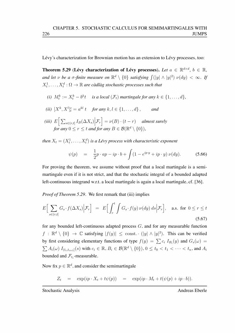
226CHAPTER 5. STOCHASTIC CALCULUS FOR SEMIMARTINGALES WITH
JUMPS
Lévy’s characterization for Brownian motion has an extension to Lévy processes, too:
Theorem 5.29 (Lévy characterization of Lévy processes). Let a ∈ Rd×d, b ∈ R,and let ν be a σ-finite measure on Rd \ 0 satisfying
´
(|y| ∧ |y|2) ν(dy) < ∞. IfX1
t , . . . , Xdt : Ω → R are càdlàg stochastic processes such that
(i) Mkt := Xk
t − bkt is a local (Ft) martingale for any k ∈ 1, . . . , d,
(ii) [Xk, X l]ct = akl t for any k, l ∈ 1, . . . , d , and
(iii) E[∑
s∈(r,t] IB(∆Xs)∣∣∣Fr
]= ν(B) · (t− r) almost surely
for any 0 ≤ r ≤ t and for any B ∈ B(Rd \ 0),
thenXt = (X1t , . . . , X
dt ) is a Lévy process with characteristic exponent
ψ(p) =1
2p · ap− ip · b+
ˆ
(1− eip·y + ip · y) ν(dy). (5.66)
For proving the theorem, we assume without proof that a local martingale is a semi-martingale even if it is not strict, and that the stochastic integral of a bounded adaptedleft-continuous integrand w.r.t. a local martingale is again a local martingale, cf. [36].
Proof of Theorem 5.29. We first remark that (iii) implies
E[ ∑
s∈(r,t]
Gs ·f(∆Xs)∣∣∣Fr
]= E
[ ˆ t
r
ˆ
Gs ·f(y) ν(dy) ds∣∣∣Fr
], a.s. for 0 ≤ r ≤ t
(5.67)for any bounded left-continuous adapted process G, and for any measurable functionf : Rd \ 0 → C satisfying |f(y)| ≤ const. · (|y| ∧ |y|2). This can be verifiedby first considering elementary functions of type f(y) =
∑ci IBi
(y) and Gs(ω) =∑
Ai(ω) I(ti,ti+1](s) with ci ∈ R, Bi ∈ B(Rd \ 0), 0 ≤ t0 < t1 < · · · < tn, and Ai
bounded and Fti-measurable.
Now fix p ∈ Rd, and consider the semimartingale
Zt = exp(ip ·Xt + tψ(p)) = exp(ip ·Mt + t(ψ(p) + ip · b)).
Stochastic Analysis Andreas Eberle

5.5. STOCHASTIC EXPONENTIALS AND CHANGE OF MEASURE 227
Noting that [Mk,M l]ct = [Xk, X l]ct = aklt by (ii), Itô’s formula yields
Zt = 1 +
ˆ t
0
Z− ip · dM +
ˆ t
0
Z− (ψ(p) + ip · b− 1
2
∑
k,l
pkplakl) dt (5.68)
+∑
(0,t]
Z−
(eip·∆X − 1− ip ·∆X
).
By (5.67) and since |eip·y − 1− ip · y| ≤ const. · (|y|∧ |y|2), the series on the right handside of (5.68) can be decomposed into a martingale and the finite variation process
At =
ˆ t
0
ˆ
Zs− (eip·y − 1− ip · y) ν(dy) ds
Therefore, by (5.68) and (5.66), (Zt) is a martingale for any p ∈ Rd. The assertion nowfollows by Lemma 2.1.
An interesting consequence of Theorem 5.29 is that a Brownian motion B and a Lévyprocess without diffusion part w.r.t. the same filtration are always independent, because[Bk, X l] = 0 for any k, l.
Exercise (Independence of Brownian motion and Lévy processes). Suppose thatBt : Ω → Rd and Xt : Ω → Rd′ are a Brownian motion and a Lévy process withcharacteristic exponent ψX(p) = −ip · b +
´
(1 − eip·y + ip · y) ν(dy) defined on thesame filtered probability space (Ω,A, P, (Ft)). Assuming that
´
(|y|∧ |y|2) ν(dy) < ∞,prove that (Bt, Xt) is a Lévy process on Rd×d′ with characteristic exponent
ψ(p, q) =1
2|p|2
Rd + ψX(q), p ∈ Rd, q ∈ R
d′.
Hence conclude that B andX are independent.
Change of measure for general semimartingales
We conclude this section with a general change of measure theorem for possibly dis-continuous semimartingales:
Theorem 5.30 (P.A.Meyer). Suppose that the probability measures P andQ are equiv-alent on Ft for any t ≥ 0 with relative density dP
dQ
∣∣∣Ft
= Zt. IfM is a local martingale
w.r.t. Q thenM −´
1Z d[Z,M ] is a local martingale w.r.t. P .
University of Bonn Summer Semester 2015

228CHAPTER 5. STOCHASTIC CALCULUS FOR SEMIMARTINGALES WITH
JUMPS
The theorem shows that w.r.t. P , (Mt) is again a semimartingale, and it yields an explicitsemimartingale decomposition for (M,P ). For the proof we recall that (Zt) is a localmartingale w.r.t. Q and (1/Zt) is a local martingale w.r.t. P .
Proof. The process ZM − [Z,M ] is a local martingale w.r.t. Q. Hence by Lemmy 2.9,the processM− 1
Z [Z,M ] is a local martingale w.r.t. P . It remains to show that 1Z [Z,M ]
differs from´
1Z d[Z,M ] by a local P -martingale. This is a consequence of the Itô
product rule: Indeed,
1
Z[Z,M ] =
ˆ
[Z,M ]− d1
Z+
ˆ
1
Z−d[Z,M ] +
[ 1Z, [Z,M ]
].
The first term on the right-hand side is a localQ-martingale, since 1/Z is aQ-martingale.The remaining two terms add up to
´
1Z d[Z,M ], because
[ 1Z, [Z,M ]
]=
∑∆
1
Z∆[Z,M ].
Remark. Note that the process´
1Z d[Z,M ] is not predictable in general. For a pre-
dictable counterpart to Theorem 5.30 cf. e.g. [36].
5.6 General predictable integrands
So far, we have considered stochastic integrals w.r.t. general semimartingales only forintegrands that are left limits of adapted càdlàg processes. This is indeed sufficientfor many applications. For some results including in particular convergence theoremsfor stochastic integrals, martingale representation theorems and the existence of localtime, stochastic integrals with more general integrands are important. In this section,we sketch the definition of stochastic integrals w.r.t. not necessarily continuous semi-martingales for general predictable integrands. For details of the proofs, we refer toChapter IV in Protter’s book [36].
Throughout this section, we fix a filtered probability space (Ω,A, P, (Ft)). Recall thatthe predictable σ-algebra P on Ω × (0,∞) is generated by all sets A × (s, t] with
Stochastic Analysis Andreas Eberle

5.6. GENERAL PREDICTABLE INTEGRANDS 229
A ∈ Fs and 0 ≤ s ≤ t, or, equivalently, by all left-continuous (Ft) adapted processes(ω, t) #→ Gt(ω). We denote by E the vector space consisting of all elementary pre-dictable processes G of the form
Gt(ω) =n−1∑
i=0
Zi(ω)I(ti,ti+1](t)
with n ∈ N, 0 ≤ t0 < t1 < · · · < tn, and Zi : Ω → R bounded and Fti-measurable.For G ∈ E and a semimartingaleX ∈ S, the stochastic integral G•X defined by
(G•X)t =
ˆ t
0
Gs dXs =n−1∑
i=0
Zi
(Xti+1∧t −Xti∧t
)
is again a semimartingale. Clearly, if A is a finite variation process then G•A has finitevariation as well.
Now suppose that M ∈ M2d (0,∞) is a square-integrable martingale. Then G•M ∈
M2d (0,∞), and the Itô isometry
||G•M ||2M2(0,∞) = E
[(ˆ ∞
0
G dM
)2]
= E
[ˆ ∞
0
G2 d[M ]
]=
ˆ
Ω×R+
G2 dP[M ] (5.69)
holds, whereP[M ](dω dt) = P (dω) [M ](ω)(dt)
is the Doléans measure of the martingale M on Ω × R+. The Itô isometry has beenderived in a more general form in Corollary 5.20, but for elementary processes it caneasily be verified directly (Excercise!).
In many textbooks, the angle bracket process ⟨M⟩ is used instead of [M ] to definestochastic integrals. The next remark shows that this is equivalent for predictable inte-grands:
Remark ([M ] vs. ⟨M⟩). LetM ∈ M2d (0,∞). If the angle-bracket process ⟨M⟩ exists
then the measures P[M ] and P⟨M⟩ coincide on predictable sets. Indeed, if C = A× (s, t]
with A ∈ Fs and 0 ≤ s ≤ t then
P[M ](C) = E [[M ]t − [M ]s ; A] = E [E[[M ]t − [M ]s|Fs] ; A]
= E [E[⟨M⟩t − ⟨M⟩s|Fs] ; A] = P⟨M⟩(C).
University of Bonn Summer Semester 2015

230CHAPTER 5. STOCHASTIC CALCULUS FOR SEMIMARTINGALES WITH
JUMPS
Since the collection of these sets C is an ∩-stable generator for the predictable σ-algebra, the measures P[M ] and P⟨M⟩ coincide on P .
Example (Doléans measures of Lévy martingales). IfMt = Xt−E[Xt]with a squareintegrable Lévy process Xt : Ω → R then
P[M ] = P⟨M⟩ = ψ′′(0) P ⊗ λ(0,∞)
where ψ is the characteristic exponent of X and λ(0,∞) denotes Lebesgue measure onR+. Hence the Doléans measure of a general Lévy martingale coincides with the onefor Brownian motion up to a multiplicative constant.
Definition of stochastic integrals w.r.t. semimartingales
We denote by H2 the vector space of all semimartingales vanishing at 0 of the formX = M + A with M ∈ M2
d (0,∞) and A ∈ FV predictable with total variationV (1)∞ (A) =
´∞0 |dAs| ∈ L2(P ). In order to define a norm on the space H2, we as-
sume without proof the following result, cf. e.g. Chapter III in Protter [36]:
Fact. Any predictable local martingale with finite variation paths is almost surely con-stant.
The result implies that the Doob-Meyer semimartingale decomposition
X = M + A (5.70)
is unique if we assume thatM is local martingale and A is a predictable finite variationprocess vanishing at 0. Therefore, we obtain a well-defined norm onH2 by setting
||X||2H2 = ||M ||2M2 + ||V (1)∞ (A)||2L2 = E
[
[M ]∞ +
(ˆ ∞
0
|dA|)2]
.
Note that the M2 norm is the restriction of the H2 norm to the subspace M2(0,∞) ⊂H2. As a consequence of (5.69), we obtain:
Corollary 5.31 (Itô isometry for semimartingales). LetX ∈ H2 with semimartingaledecomposition as above. Then
||G•X||H2 = ||G||X for any G ∈ E , where
Stochastic Analysis Andreas Eberle

5.6. GENERAL PREDICTABLE INTEGRANDS 231
||G||2X := ||G||2L2(P[M])+∣∣∣∣∣∣ˆ ∞
0
|G| |dA|∣∣∣∣∣∣2
L2(P ).
Hence the stochastic integral J : E → H2, JX(G) = G•X , has a unique isometricextension to the closure EX of E w.r.t. the norm || · ||X in the space of all predictableprocesses in L2(P[M ]).
Proof. The semimartingale decomposition X = M + A implies a corresponding de-composition G•X = G•M + G•A for the stochastic integrals. One can verify thatfor G ∈ E , G•M is in M2
d (0,∞) and G•A is a predictable finite variation process.Therefore, and by (5.69),
||G•X||2H2 = ||G•M ||2M2 + ||V (1)∞ (G•A)||2L2 = ||G||2L2(P[M])
+∣∣∣∣∣∣ˆ
|G| |dA|∣∣∣∣∣∣2
L2(P ).
The Itô isometry yields a definition of the stochastic integral G•X for G ∈ EX . ForG = H− with H càdlàg and adapted, this definition is consistent with the definitiongiven above since, by Corollary 5.20, the Itô isometry also holds for the integrals definedabove, and the isometric extension is unique. The class EX of admissible integrands isalready quite large:
Lemma 5.32. EX contains all predictable processes G with ||G||X < ∞.
Proof. We only mention the main steps of the proof, cf. [36] for details:1) The approximation of bounded left-continuous processes by elementary predictableprocesses w.r.t. || · ||X is straightforward by dominated convergence.
2) The approximability of bounded predictable processes by bounded left-continuousprocesses w.r.t. || · ||X can be shown via the Monotone Class Theorem.
3) For unbounded predictable G with ||G||X < ∞, the processes Gn := G · IG≤n,n ∈ N, are predictable and bounded with ||Gn −G||X → 0.
Localization
Having defined G•X for X ∈ H2 and predictable integrands G with ||G||X < ∞, thenext step is again a localization. This localization is slightly different than before, be-cause there might be unbounded jumps at the localizing stopping times. To overcome
University of Bonn Summer Semester 2015

232CHAPTER 5. STOCHASTIC CALCULUS FOR SEMIMARTINGALES WITH
JUMPS
this difficulty, the process is stopped just before the stopping time T , i.e., at T−. How-ever, stopping at T− destroys the martingale property if T is not a predictable stoppingtime. Therefore, it is essential that we localize semimartingales instead of martingales!
For a semimartingaleX and a stopping time T we define the stopped process XT− by
XT−t =
⎧⎪⎪⎪⎨
⎪⎪⎪⎩
Xt for t < T,
XT− for t ≥ T > 0,
0 for T = 0.
The definition for T = 0 is of course rather arbitrary. It will not be relevant below, sincewe are considering sequences (Tn) of stopping times with Tn ↑ ∞ almost surely. Westate the following result from Chapter IV in [36] without proof.
Fact. If X is a semimartingale with X0 = 0 then there exists an increasing sequence(Tn) of stopping times with sup Tn = ∞ such thatXTn− ∈ H2 for any n ∈ N.
Now we are ready to state the definition of stochastic integrals for general predictableintegrands w.r.t. general semimartingales X . By setting G•X = G•(X − X0) we mayassumeX0 = 0.
Definition. Let X be a semimartingale with X0 = 0. A predictable process G is calledintegrable w.r.t. X iff there exists an increasing sequence (Tn) of stopping times suchthat supTn = ∞ a.s., and for any n ∈ N,XTn− ∈ H2 and ||G||XTn− < ∞.
If G is integrable w.r.t.X then the stochastic integral G•X is defined by
(G•X)t =
ˆ t
0
Gs dXs =
ˆ t
0
Gs dXTn−s for any t ∈ [0, Tn), n ∈ N.
Of course, one has to verify that G•X is well-defined. This requires in particular alocality property for the stochastic integrals that are used in the localization. We do notcarry out the details here, but refer once more to Chapter IV in [36].
Exercise (Sufficient conditions for integrability of predictable processes).
1) Prove that if G is predictable and locally bounded in the sense that GTn is boundedfor a sequence (Tn) of stopping times with Tn ↑ ∞, then G is integrable w.r.t. anysemimartingaleX ∈ S.
Stochastic Analysis Andreas Eberle

5.6. GENERAL PREDICTABLE INTEGRANDS 233
2) Suppose that X = M + A is a continuous semimartingale with M ∈ Mlocc and
A ∈ FVc. Prove that G is integrable w.r.t.X if G is predictable andˆ t
0
G2s d[M ]s +
ˆ t
0
|Gs| |dAs| < ∞ a.s. for any t ≥ 0.
Properties of the stochastic integral
Most of the properties of stochastic integrals can be extended easily to general pre-dictable integrands by approximation with elementary processes and localization. Theproof of Property (2) below, however, is not trivial. We refer to Chapter IV in [36] fordetailed proofs of the following basic properties:
(1) The map (G,X) #→ G•X is bilinear.
(2) ∆(G•X) = G∆X almost surely.
(3) (G•X)T = (G I[0,T ])•X = G•XT .
(4) (G•X)T− = G•XT−.
(5) G•(G•X) = (GG)•X .
In all statements,X is a semimartingale,G is a process that is integrable w.r.t.X , T is astopping time, and G is a process such that GG is also integrable w.r.t.X . We state theformula for the covariation of stochastic integrals separately below, because its proof isbased on the Kunita-Watanabe inequality, which is of independent interest.
Exercise (Kunita-Watanabe inequality). Let X, Y ∈ S, and let G,H be measurableprocesses defined on Ω × (0,∞) (predictability is not required). Prove that for anya ∈ [0,∞] and p, q ∈ [1,∞] with 1
p +1q = 1, the following inequalities hold:
ˆ a
0
|G||H| |d[X, Y ]| ≤(ˆ a
0
G2 d[X ])1/2 (ˆ a
0
H2 d[Y ])1/2
, (5.71)
E[ˆ a
0
|G||H| |d[X, Y ]|]
≤∣∣∣∣∣∣(ˆ a
0
G2 d[X ])1/2∣∣∣
∣∣∣Lp
∣∣∣∣∣∣(ˆ a
0
H2 d[Y ])1/2∣∣∣
∣∣∣Lq.
(5.72)Hint: First consider elementary processes G,H .
University of Bonn Summer Semester 2015

234CHAPTER 5. STOCHASTIC CALCULUS FOR SEMIMARTINGALES WITH
JUMPS
Theorem 5.33 (Covariation of stochastic integrals). For any X, Y ∈ S and any pre-dictable process G that is integrable w.r.t.X ,
[ˆG dX, Y
]=
ˆ
G d[X, Y ] almost surely. (5.73)
Remark. IfX and Y are local martingales, and the angle-bracket process ⟨X, Y ⟩ exists,then also ⟨ˆ
G dX, Y⟩
=
ˆ
G d⟨X, Y ⟩ almost surely.
Proof of Theorem 5.33. We only sketch the main steps briefly, cf. [36] for details. Firstly,one verifies directly that (5.73) holds for X, Y ∈ H2 and G ∈ E . Secondly, forX, Y ∈ H2 and a predictable process G with ||G||X < ∞ there exists a sequence(Gn) of elementary predictable processes such that ||Gn −G||X → 0, and
[ˆGn dX, Y
]=
ˆ
Gn d[X, Y ] for any n ∈ N.
As n → ∞,´
Gn dX →´
G dX in H2 by the Itô isometry for semimartingales, andhence [ ˆ
Gn dX, Y]
−→[ ˆ
G dX, Y]
u.c.p.
by Corollary 5.14. Moreover,ˆ
Gn d[X, Y ] −→ˆ
G d[X, Y ] u.c.p.
by the Kunita-Watanabe inequality. Hence (5.73) holds for G as well. Finally, by local-ization, the identity can be extended to general semimartingalesX, Y and integrands Gthat are integrable w.r.t.X .
An important motivation for the extension of stochastic integrals to general predictableintegrands is the validity of a Dominated Convergence Theorem:
Theorem 5.34 (Dominated Convergence Theorem for stochastic integrals). Supposethat X is a semimartingale with decomposition X = M + A as above, and let Gn,n ∈ N, and G be predictable processes. If
Gnt (ω) −→ Gt(ω) for any t ≥ 0, almost surely,
Stochastic Analysis Andreas Eberle

5.6. GENERAL PREDICTABLE INTEGRANDS 235
and if there exists a process H that is integrable w.r.t. X such that |Gn| ≤ H for anyn ∈ N, then
Gn•X −→ G•X u.c.p. as n → ∞.
If, in addition to the assumptions above, X is inH2 and ||H||X < ∞ then even
||Gn•X −G•X||H2 −→ 0 as n → ∞.
Proof. We may assume G = 0, otherwise we consider Gn − G instead of Gn. Nowsuppose first that X is inH2 and ||H||X < ∞. Then
||Gn||2X = E[ˆ ∞
0
|Gn|2 d[M ] +(ˆ ∞
0
|Gn| |dA|)2]
−→ 0
as n → ∞ by the Dominated Convergence Theorem for Lebesgue integrals. Hence bythe Itô isometry,
Gn•X −→ 0 in H2 as n → ∞.
The general case can now be reduced to this case by localization, whereH2 convergenceis replaced by the weaker ucp-convergence.
We finally remark that basic properties of stochastic integrals carry over to integralswith respect to compensated Poisson point processes. We refer to the monographs byD.Applebaum [5] for basics, and to Jacod & Shiryaev [24] for a detailed study. We onlystate the following extension of the associative law, which has already been used in thelast section:
Exercise (Integration w.r.t. stochastic integrals based on compensated PPP). Sup-pose that H : Ω × R+ × S → R is predictable and square-integrable w.r.t. P ⊗ λ⊗ ν,and G : Ω× R+ → R is a bounded predictable process. Show that if
Xt =
ˆ
(0,t]×S
Hs(y) N(ds dy)
thenˆ t
0
Gs dXs =
ˆ
(0,t]×S
GsHs(y) N(ds dy).
Hint: Approximate G by elementary processes.
University of Bonn Summer Semester 2015

Bibliography
[1]
[2]
[3] Sur l’équation de Kolmogoroff, par W. Doeblin. Éditions Elsevier, Paris, 2000. C.R. Acad. Sci. Paris Sér. I Math. 331 (2000), Special Issue.
[4] Robert J. Adler and Jonathan E. Taylor. Random fields and geometry. SpringerMonographs in Mathematics. Springer, New York, 2007.
[5] David Applebaum. Lévy Processes and Stochastic Calculus. Cambridge UP, Cam-bridge, 2004.
[6] Ole E. Barndorff-Nielsen. Processes of normal inverse Gaussian type. FinanceStoch., 2(1):41–68, 1998.
[7] Richard F. Bass. Stochastic Processes. Cambridge University Press, Cambridge,2011.
[8] Jean Bertoin. Lévy Processes. Cambridge UP, Cambridge, 1998.
[9] Jean-Michel Bismut. Large deviations and the Malliavin calculus. Birkhaeuser,Boston, 1994.
[10] Amir Dembo and Ofur Zeitouni. Large Deviations Techniques and Applications.Springer, 1998, Berlin.
[11] Frank den Hollander. Large Deviations. American Mathematical Society, Provi-dence, 2008.
236

BIBLIOGRAPHY 237
[12] Andreas Eberle. Markov processes.http://www.uni-bonn.de/~eberle/MarkovProcesses/MPSkript.pdf,2009.
[13] Andreas Eberle. Wahrscheinlichkeitstheorie und Stochastische Prozesse.http://www.uni-bonn.de/~eberle/StoPr/WthSkriptneu.pdf,2010.
[14] Andreas Eberle. Introduction to Stochastic Analysis.http://www.uni-bonn.de/~eberle/StoAn1011/StoAnSkriptneu.pdf,2011.
[15] David Elworthy. On the Geometry of Diffusion Operators and Stochastic Flows.Springer, 1999, Berlin.
[16] Stewart N. Ethier and Thomas G. Kurtz. Markov Processes. Wiley-Interscience,Hoboken, NJ, 2005.
[17] William Feller. Introduction to Probability Theory and Its Applications. Wiley,New York, 1957.
[18] Peter K. Friz and Martin Hairer. A course on rough paths. Universitext. Springer,Cham, 2014. With an introduction to regularity structures.
[19] Peter K. Friz and Nicolas Victoir.Multidimensional Stochastic Processes as RoughPaths. Cambridge UP, Cambridge, 2010.
[20] W. Hackenbroch and A. Thalmaier. Stochastic Analysis. Teubner, 1991.
[21] Martin Hairer. On malliavin’s proof of hörmander’s theorem. Bull. Sci. Math.,135(6-7):650–666, 2011.
[22] Elton Hsu. Stochastic Analysis on Manifolds. Oxford University Press, Oxford,2002.
[23] Nobuyuki Ikeda and Takehiko Ed. Watanabe. Stochastic Differential Equationsand Diffusion Processes. North-Holland, Amsterdam, 1981.
University of Bonn Summer Semester 2015

238 BIBLIOGRAPHY
[24] Jean Jacod and Albert Shiryaev. Limit Theorems for Stochastic Processes.Springer, Berlin, 2003.
[25] Ioannis Karatzas and Steven E. Shreve. Brownian motion and stochastic calculus.Springer, New York, 2010.
[26] Peter E. Kloeden and Eckhard Platen. Numerical solution of stochastic differen-tial equations, volume 23 of Applications of Mathematics (New York). Springer-Verlag, Berlin, 1992.
[27] Hiroshi Kunita. Stochastic Flows and Stochastic Differential Equations. Cam-bridge University Press, Cambridge, 1997.
[28] Andreas Kyprianou. Introductory Lectures on Fluctuations of Lévy Processes withApplications. Springer, Berlin, 2006.
[29] Terry J. Lyons. Differential Equations Driven by Rough Paths, Ecole d’Eté deProbabilités de Saint-Flour XXXIV. Springer, 2004.
[30] Zhi-Ming Ma and Michael Röckner. Introduction to the Theory of (Non-Symmetric) Dirichlet Forms. Springer, Berlin, 1992.
[31] Dilip B. Madan and Eugene Seneta. The variance gamma model for share marketreturns. Journal of Business, 63(4):511–524, 1990.
[32] Paul Malliavin. Stochastic Analysis. Springer, Berlin, 2002.
[33] G. N.Milstein andM. V. Tretyakov. Stochastic numerics for mathematical physics.Scientific Computation. Springer-Verlag, Berlin, 2004.
[34] David Nualart. The Malliavin Calculus and Related Topics. Springer, Berlin,2006.
[35] Giuseppe Da Prato. Introduction to Stochastic Analysis and Malliavin Calculus.Edizioni della Normale, Pisa, 2009.
[36] Philip E. Protter. Stochastic Integration and Differential Equations. Springer,Berlin, 2005.
Stochastic Analysis Andreas Eberle

BIBLIOGRAPHY 239
[37] Daniel Revuz and Marc Yor. Continuous martingales and Brownian motion.Springer, Berlin, 2005.
[38] L. C. G. Rogers and David Williams. Diffusions, Markov processes and martin-gales, Vol. 2: Ito calculus. Cambridge UP, Camebridge, 2008.
[39] Steven E. Shreve. Stochastic calculus for finance. II. Springer Finance. Springer-Verlag, New York, 2004. Continuous-time models.
[40] Daniel W. Stroock and S.R. S. Varadhan. Multidimensional Diffusion Processes.Springer, Berlin, 2005.
[41] Shinzo Watanabe. Lectures on stochastic differential equations and Malliavin cal-culus. Springer, Berlin, 1984.
University of Bonn Summer Semester 2015