Stimulating Housing Markets∗

David BergerNorthwestern University and NBER

david.berger@northwestern.edu

Nicholas TurnerOffice of Tax Analysis

nicholas.turner@treasury.gov

Eric ZwickChicago Booth and NBERezwick@chicagobooth.edu

February 2018

Abstract

We study temporary policies designed to address capital overhang by inducing assetdemand from buyers in the private market. Using difference-in-differences and regressionkink research designs, we find the First-Time Homebuyer Credit caused home sales to in-crease 412,000-610,000 (8.1-12.1%) nationally, median home prices to increase $2,390(1.08%) per standard deviation increase in program exposure, and the transition rate intohomeownership to increase by 53%. We find little evidence that the policy response re-versed immediately; instead, demand comes from several years in the future. The programsped the process of reallocating homes from distressed sellers to high-value buyers. Thisstabilizing benefit likely exceeded the program’s stimulative effects.

∗We thank Andrew Abel, Gene Amromin, Michael Best, Jediphi Cabal, Anthony DeFusco, Paul Goldsmith-Pinkham, Adam Guren, Erik Hurst, Anil Kashyap, Amir Kermani, Ben Keys, Henrik Kleven, Pat Langetieg, AdamLooney, Janet McCubbin, Matt Notowidigdo, Christopher Palmer, Jonathan Parker, Amit Seru, Isaac Sorkin, Jo-hannes Stroebel, Amir Sufi, Joe Vavra, Rob Vishny, Owen Zidar and seminar and conference participants forcomments, ideas, and help with data. Tianfang Cui, Prab Upadrashta, Iris Song, and Caleb Wroblewski providedexcellent research assistance. The views expressed here are ours and do not necessarily reflect those of the USTreasury Office of Tax Analysis, nor the IRS Office of Research, Analysis and Statistics. Zwick gratefully acknowl-edges financial support from the Neubauer Family Foundation, Initiative on Global Markets, and Booth School ofBusiness at the University of Chicago.

1

A classic debate in economics concerns how policy should respond to periods of capital

overhang following investment booms (Hayek, 1931; Keynes, 1936). When booms coincide

with credit expansions, high-valuation potential buyers often cannot finance distressed asset

purchases in the subsequent slump (Shleifer and Vishny, 1992). In this case, an overhang leads

to fire sales and inefficient liquidation, amplifying the slump through debt-deflation dynam-

ics and creating a role for welfare-improving policy intervention (Fisher, 1933; Kiyotaki and

Moore, 1997; Lorenzoni, 2008; Eggertsson and Krugman, 2012).

This problem reemerged in the aftermath of the Great Recession, with the housing market

suffering extraordinary distress as shown in Figure 1. As house price growth slowed, a shortage

of prospective buyers for new homes caused housing inventory to double from 2004 to mid-

2006 and remain at historic levels in 2007 and 2008. The boom coincided with a rapid and

widespread increase in household debt secured by real estate (Mian and Sufi, 2015). When

house prices began to fall, defaults, foreclosures, and further downward pressure on prices

ensued (Campbell, Giglio and Pathak, 2011; Mian, Sufi and Trebbi, 2015; Guren and McQuade,

2015). By mid-2008, a dramatic shift in the composition of home sales had taken place, with

nearly forty percent of home sales classified as distressed or foreclosure sales and vacancies at

or near all-time highs.

The debt-induced overhang in the housing market prompted many policy proposals and re-

sponses, primarily in the form of debt renegotiation interventions designed to repair household

balance sheets, government asset purchase programs designed to support financial markets,

and monetary and fiscal policy designed to spur demand growth.1 However, these policies do

not directly target the problem of capital overhang, nor do they promote reallocation when

assets are no longer in the hands of their first-best users. And despite a large theoretical liter-

ature describing the welfare costs of overhang-induced fire sales, there is little empirical work

evaluating policies which target overhang.

This paper evaluates a $20 billion policy designed to induce demand for housing through

providing temporary tax incentives for buyers in the private market. The policy we study,

the First-Time Homebuyer Credit (FTHC), was a temporary tax incentive for new homebuy-

ers between 2008 and 2010. We combine data from administrative tax records with trans-

action deeds data to measure program exposure and housing market outcomes for approxi-

mately 9,000 ZIP codes, which account for 69 percent of the U.S. population in 2007. We

1Diamond and Rajan (2011), French, Baily, Campbell, Cochrane, Diamond, Duffie, Kashyap, Mishkin, Rajan,Scharfstein et al. (2010), Shleifer and Vishny (2010a), Hanson, Kashyap and Stein (2011), and Eberly and Kr-ishnamurthy (2014) discuss potential policy solutions. A recent empirical literature aims to evaluate some of theprograms that address debt overhang in the Great Recession (Agarwal, Amromin, Ben-David, Chomsisengphet,Piskorski and Seru, 2017; Agarwal, Amromin, Chomsisengphet, Piskorski, Seru and Yao, 2017).

2

use difference-in-differences and regression kink research designs to estimate the effect of the

policy on home sales, homeownership, and the housing market more broadly. We then ask

whether the policy induced reallocation of underutilized homes and whether this reallocation

stabilized housing market health.

We present five main findings. First, the policy proved effective at spurring home sales. We

estimate the FTHC raised home sales during the policy period by 412,000 to 610,000 nationally.

Second, we find little evidence that the surge in home sales induced by the credit reversed

immediately following the policy period. Instead, demand appears to come from several years

in the future. Third, the policy was effective at increasing homeownership rates. We estimate

the causal effect of the FTHC on the likelihood of being a first-time homebuyer for an individual

and find that receiving the full credit causes this propensity to increase by over 50%. Fourth,

the policy response came primarily in the form of existing home sales, implying the direct

stimulative effects of the program were small ($5.4 to $9.6 billion). Fifth, we present evidence

that the program likely accelerated the process of reallocation from low-value sellers to high-

value buyers, and the health of the housing market, as reflected in house prices, improved

accordingly. Our best estimate suggests the policy increased the median home price by $2,390

(1.08%) per standard deviation of exposure. A back-of-the-envelope calculation suggests the

consumption response to the increase in house prices was likely much larger than the policy’s

direct stimulative effect.

The first part of the paper documents the effect of the FTHC on home sales and transitions

into homeownership and presents a number of robustness tests. Our difference-in-differences

design compares ZIP codes at the same point in time whose exposure to the program differs.

We define program exposure based on the number of potential first-time homebuyers in a ZIP

code, proxied by the share of people in that ZIP in the year 2000 who are first-time homebuyers.

We assume places with few potential first-time homebuyers serve as a “control group” because

the policy does not induce many people to buy in these places. The key threat to this design

is the possibility that time-varying, place-specific shocks are correlated with our measures of

program exposure.

We assess this threat in six ways. First, graphical inspection of parallel trends indicates

smooth pre-trends, clear breaks during the policy period and spikes at policy expiration due

to the temporary nature of the policy, and a reversion to pre-trends in the post-policy period.

Second, estimates are robust to the inclusion of CBSA-by-time fixed effects, which is our default

specification. We also include explicit controls for subprime households and exposure to the

major contemporaneous policy programs, including FHA’s mortgage limit expansion and the

3

HARP and HAMP programs, and show that controlling for these potential confounds does not

affect our results. Third, our results are consistent across different specifications, with varying

control sets, weighting schemes, and sample definitions. Fourth, we exploit the fact that the

subsidy is less generous relative to home prices in more expensive areas: our results are driven

by low price ZIP codes where the value of the subsidy is greatest. Fifth, the age distribution

of first-time homebuyers shifts considerably toward younger buyers in 2009 and subsequently

reverts to its long run average, a pattern that cannot be explained by place-by-time trends.

Last, our results are driven by activity in the “starter home” market, with sales in homes with

1 to 3 bedrooms responding strongly while sales in the 4+ bedrooms market respond little.

This test provides a within-time placebo that complements the pre- and post-policy trends in

confirming the design’s robustness.

In addition to the market-level evidence from our difference-in-difference research design,

we also estimate the response at the individual level using a sharp regression kink design. We

implement this approach using detailed population administrative tax data and exploiting the

income phase-out range of the FTHC. We estimate the intention-to-treat effect, as we impute

the value of the FTHC for all observations and relate the slope change of this potential FTHC

to the slope change in the probability of being a first-time homebuyer. The causal effect of the

FTHC on being a first-time homebuyer is the ratio of the slope change in the probability of

being a first-time homebuyer and the slope change in the potential FTHC. To the best of our

knowledge, this is the first paper to estimate this elasticity, which is an important input in the

design of government policies aimed at increasing homeownership rates. Using this research

design, we estimate the FTHC increased the rate of transition into homeownership 0.76%

relative to a baseline rate of 1.43%. Our estimates imply an aggregate effect on purchases

between 520,000 and 610,000, matching estimates from our cross-sectional approach despite

using a very different identification strategy.

In the second part of the paper, we explore the value of the FTHC program as housing

market stabilizer. We start by examining the effect of the policy on house prices following the

same empirical strategy we used to analyze the effect on home sales. Consistent with a real-

location toward higher utility users, we find the program increased house prices significantly

in a variety of data sets. In our preferred specification, we find that a one standard devia-

tion increase in exposure to the program caused the median home to appreciate by $2,390.

We also show that aggregate repeat-sale price indices likely understate the true effect of the

program because they smooth high frequency price changes and exclude a large fraction of

policy-relevant transactions.

4

Relying on the detail available in housing transaction data, we show next that many trans-

actions during the policy period involved sales by investors and institutional sellers, who were

likely to be low-value users of the assets. More than a quarter of the homes sold during this

time came out of foreclosure or real estate owned (REO) portfolios from financial institutions

and government sponsored entities. Similarly, sixteen percent of homes were built in the pre-

ceding one to three years and sold by builders or developers during the policy period, and thus

were likely vacant before being sold.

Furthermore, many buyers induced by the program were constrained by down payment

requirements that the credit helped relax.2 During 2009 alone, more than 780,000 homebuyers

took advantage of low down payment loans insured by the Federal Housing Administration

(FHA), despite these loans carrying significantly higher net present value costs. Furthermore,

53 percent of all credit claims and 57 percent of claims by buyers aged 30 and below came

via amended returns, suggesting the urgency with which financially constrained buyers sought

the credit. Down payment constraints can also explain why we fail to find evidence of a sharp

reversal after the policy expires: absent the policy, induced buyers must wait until they have

accumulated the necessary down payment as savings. These facts are consistent with the idea

that debt-induced capital overhangs are times when potential high-value buyers are unable to

finance welfare-improving reallocations in the absence of policy intervention.

Last, we examine the stability of the policy-induced reallocation and find that, although

many policy period buyers bought with high loan-to-value ratios, they were not more likely to

default in the subsequent three years than other cohorts of homebuyers. The fact that housing

demand was being pulled from years rather than months in the future lends further evidence

of the program’s medium-run stabilizing effects.

Section 1 provides background information on the FTHC program. Section 2 describes

the tax and housing market data. Section 3 describes our main empirical strategy. Section

4 provides evidence on the effect of the policy on home sales and homeownership. Section

5 explores the effect of the policy on reallocation and prices. Section 6 uses estimates from

Sections 4 and 5 to study the aggregate direct and indirect effects of the policy. Section 7

concludes.

Related literature. Our paper contributes to the empirical literature on policy responses to

distress in debt markets, especially policies motivated by the Great Recession (Agarwal, Am-

romin, Ben-David, Chomsisengphet, Piskorski and Seru, 2017; Agarwal, Amromin, Chomsisen-

2We explore this fact and the implications for theories of intertemporal demand for durables in a follow-uppaper (Berger, Cui, Turner and Zwick, 2017).

5

gphet, Piskorski, Seru and Yao, 2017). Relative to these, we focus on how policy can stabilize

prices during potential fire sales and address capital overhang by accelerating reallocation,

which is typically slow during periods of industry decline or macroeconomic weakness (Ramey

and Shapiro, 2001; Eisfeldt and Rampini, 2006; Rognlie, Shleifer and Simsek, 2014). Our

paper complements studies that estimate the effects of fiscal stimulus by contributing a new

analysis of an important durable goods stimulus program (Adda and Cooper, 2000; House and

Shapiro, 2008; Mian and Sufi, 2012; Berger and Vavra, 2015; Zwick and Mahon, 2017; Green,

Melzer, Parker and Rojas, 2016). Taken together, these studies demonstrate how the reversal of

durable goods stimulus programs depends on which activity is targeted and who the marginal

buyers are.

A closely related paper by Best and Kleven (2017) studies the effect of stamp duty tax

notches and temporary tax holidays on housing sales in the UK, with a focus on these policies

as economic stimulus. This paper finds similar effects on home sales that only partially reverse

post-policy. Our paper differs in four important respects. First, their research design does

not permit study of the broader effects of these policies on housing market health. A key

contribution of our paper is documenting that the FTHC had powerful effects on market-level

house prices and promoted reallocation of underused housing, which is evidence that the policy

played an important role as a housing market stabilizer during the Great Recession. Second, the

policy we study focused explicitly on first-time homebuyers. Thus, we can identify the causal

effect of a temporary tax change on transitions into homeownership, rather than the effect on

overall transaction volume. Credible estimates of the elasticity for first-time homebuyers are

important for evaluating the many policies governments use to encourage homeownership.

Third, we bring to bear data on the buyers and sellers during the policy period, which yields a

more detailed analysis of the mechanisms underlying the estimated response. Fourth, we each

study these questions using different research designs with different strengths and weaknesses.

In particular, they use a bunching research design and a difference-in-differences design based

on house price cutoffs, while we use cross-market variation in program exposure, a cohort

analysis of the age distribution of first-time buyers, and a regression kink design based on

income cutoffs.

Other closely related papers are Brogaard and Roshak (2011), Hembre (2015), and Dynan,

Gayer and Plotkin (2013), who conduct policy evaluations of the FTHC and find mixed or small

effects. Brogaard and Roshak (2011) find that quantity was not noticeably affected and that

prices rose only temporarily. In contrast, Hembre (2015) finds large quantity responses and

negligible price effects. Dynan, Gayer and Plotkin (2013) conclude that the credit had “at best,

6

small and mostly temporary effects on housing activity,” identifying small positive effects on

home sales and prices. While we also exploit the FTHC as a natural experiment, our approach

yields stronger results, which are likely driven by the more granular data and sharper design

we use. Most substantively, we emphasize and study the market-stabilizing role of the program

and provide evidence suggesting this role was first order.

1 Policy Background

The First-Time Homebuyer Credit (FTHC) was a temporary stimulus policy introduced in the

U.S. between 2008 and 2010 with the aim of supporting weak housing markets. There were

three versions of the program. The first version, enacted on July 30, 2008, in the Housing

and Economic Recovery Act, provided an interest-free loan of up to $7,500 on qualifying home

purchases made between April 9, 2008, and June 30, 2009. To be eligible for the maximum

value of this version of the credit, a single (married) taxpayer needed a modified adjusted gross

income (AGI) below $75,000 ($150,000) and must not have owned a principal residence dur-

ing the 3-year period preceding the purchase date. Taxpayers at higher incomes were eligible

for a smaller credit, as the maximum FTHC phased out over the next $20,000 of AGI.

The second version of the credit was enacted on February 17, 2009, as part of the American

Recovery and Reinvestment Act. The policy window was extended to include purchases made

up to November 30, 2009. Importantly, the maximum credit increased to $8,000 (equal to

10% of sale price up to $8,000) and was changed from an interest-free loan to a refundable

tax credit. This feature significantly increased the value of the credit to potential homebuyers.

The third version of the credit was enacted on November 7, 2009, as part of the Worker,

Homeownership, and Business Assistance Act. The policy window was extended to include

purchases closing before July 1, 2010.3 The third version also raised the income limits so

that eligibility began to phase out for a single (married) taxpayer with modified adjusted gross

income above $125,000 ($225,000). For each version of the credit, the eligible amount phased

out linearly over a $20,000 range.

To claim the credit, tax filers needed to note the FTHC on their income tax returns (Form

1040) and attach an additional credit claim (Form 5405). Claimants also needed to provide

documentation demonstrating the purchase of a home during the policy window, together

with mailing documents supporting the claim’s eligibility for the credit to the appropriate IRS

3The expanded policy also added a $6,500 Long-Time Homebuyer Credit (LTHC). To qualify for the LTHC, anindividual must have owned and used the residence as his or her principal residence for a consecutive five yearperiod during the eight years prior to the date of the new purchase.

7

office.4 To accelerate payment, filers could amend previously filed tax returns, for example by

amending the 2008 tax return for a home bought in 2009.

We focus on the second and third versions of this policy. We do so for three reasons. First,

these versions of the credit were considerably more generous and thus more likely to induce

new purchases. Assuming a 3 percent real rate of return, the interest free loan was worth

$1,400 dollars in present value; the later versions were worth 5.7 times as much. Second, the

later versions of the policy were more broadly publicized at the time of enaction and thus were

more likely to induce changes in behavior rather than retrospective claims for past purchases.

Third, unlike the first loan-based version of the credit, the second and third versions were eligi-

ble to contribute to down payments, following lender guidance by the Department of Housing

and Urban Development (see Mortgagee Letter 2009-15).5

Figure 2 presents time series plots that justify our focus on the second and third versions.

Panel (a) presents existing home sales on a seasonally adjusted annual basis from the National

Association of Realtors and shows that there were significant aggregate spikes at the end of

the second and third extensions of the policy. Panels (b) and (c) confirm these spikes within

our analysis sample, using seasonally adjusted home sales from DataQuick. Panel (d) plots

Google search trend data for the terms “first time home buyer” and “home buyer credit” along

with vertical markers for policy events. Interest in these credits spiked at the beginning of the

second extension, remained elevated throughout both policy periods, and then declined after

the end of the third version.

Congress passed the FTHC with the explicit purpose of inducing demand for homes at a time

of unusual weakness and helping to spur the economic recovery. In the respective words of

Senators Cardin, Shelby, and Salazar, the program would “help the housing market,” it would

“help get homebuilders and the housing industry back on track,” and it would “help us get rid

of the glut we currently have in the market.”6 We evaluate this policy as both housing market

stabilizer and fiscal stimulus. As stabilizer, the key questions are whether the policy promoted

reallocation of underutilized assets from distressed sellers to constrained, higher value buyers,

and whether this reallocation affected house prices. As stimulus, the key question is whether

the policy contributed to economic activity by inducing new home sales or through the fees

and complementary purchases that accompany an existing home sale. The non-random timing

of the policy motivates the cross-sectional approach we pursue to separate the effect of the

4Such documents could include the settlement statement (typically Form HUD-1), executed retail sales contract(for mobile homes), or certificate of occupancy (for new construction).

5Appendix Table A.1 estimates the effect of version one and shows modest positive effects.6Congressional Record, Vol. 154, No. 52 (April 3, 2008) and Congressional Record, Vol. 154, No. 124 (July

26, 2008).

8

program from other factors affecting housing markets at this time.

2 Data

This section presents an overview of the data sources for our analysis, discusses construction

of key variables, and presents summary statistics. Appendix A presents additional information

on the data build process, detailed variable definitions, and supplementary sample statistics.

2.1 Data Sources

We develop our measure of ex ante program exposure using the population of de-identified

individual tax return data, available over the time period between 1998 and 2013. These data

include information about the age, earnings, marital status, number of dependents, and tax

filing ZIP code reported on the income tax return.

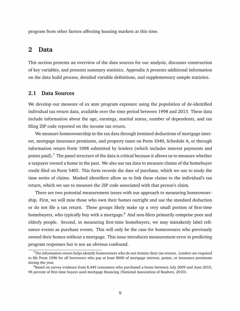
We measure homeownership in the tax data through itemized deductions of mortgage inter-

est, mortgage insurance premiums, and property taxes on Form 1040, Schedule A, or through

information return Form 1098 submitted by lenders (which includes interest payments and

points paid).7 The panel structure of the data is critical because it allows us to measure whether

a taxpayer owned a home in the past. We also use tax data to measure claims of the homebuyer

credit filed on Form 5405. This form records the date of purchase, which we use to study the

time series of claims. Masked identifiers allow us to link these claims to the individual’s tax

return, which we use to measure the ZIP code associated with that person’s claim.

There are two potential measurement issues with our approach to measuring homeowner-

ship. First, we will miss those who own their homes outright and use the standard deduction

or do not file a tax return. These groups likely make up a very small portion of first-time

homebuyers, who typically buy with a mortgage.8 And non-filers primarily comprise poor and

elderly people. Second, in measuring first-time homebuyers, we may mistakenly label refi-

nance events as purchase events. This will only be the case for homeowners who previously

owned their homes without a mortgage. This issue introduces measurement error in predicting

program responses but is not an obvious confound.

7The information return helps identify homeowners who do not itemize their tax returns. Lenders are requiredto file Form 1098 for all borrowers who pay at least $600 of mortgage interest, points, or insurance premiumsduring the year.

8Based on survey evidence from 8,449 consumers who purchased a home between July 2009 and June 2010,96 percent of first-time buyers used mortgage financing (National Association of Realtors, 2010).

9

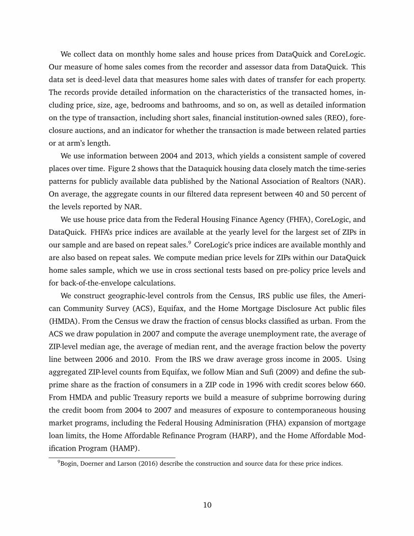
We collect data on monthly home sales and house prices from DataQuick and CoreLogic.

Our measure of home sales comes from the recorder and assessor data from DataQuick. This

data set is deed-level data that measures home sales with dates of transfer for each property.

The records provide detailed information on the characteristics of the transacted homes, in-

cluding price, size, age, bedrooms and bathrooms, and so on, as well as detailed information

on the type of transaction, including short sales, financial institution-owned sales (REO), fore-

closure auctions, and an indicator for whether the transaction is made between related parties

or at arm’s length.

We use information between 2004 and 2013, which yields a consistent sample of covered

places over time. Figure 2 shows that the Dataquick housing data closely match the time-series

patterns for publicly available data published by the National Association of Realtors (NAR).

On average, the aggregate counts in our filtered data represent between 40 and 50 percent of

the levels reported by NAR.

We use house price data from the Federal Housing Finance Agency (FHFA), CoreLogic, and

DataQuick. FHFA’s price indices are available at the yearly level for the largest set of ZIPs in

our sample and are based on repeat sales.9 CoreLogic’s price indices are available monthly and

are also based on repeat sales. We compute median price levels for ZIPs within our DataQuick

home sales sample, which we use in cross sectional tests based on pre-policy price levels and

for back-of-the-envelope calculations.

We construct geographic-level controls from the Census, IRS public use files, the Ameri-

can Community Survey (ACS), Equifax, and the Home Mortgage Disclosure Act public files

(HMDA). From the Census we draw the fraction of census blocks classified as urban. From the

ACS we draw population in 2007 and compute the average unemployment rate, the average of

ZIP-level median age, the average of median rent, and the average fraction below the poverty

line between 2006 and 2010. From the IRS we draw average gross income in 2005. Using

aggregated ZIP-level counts from Equifax, we follow Mian and Sufi (2009) and define the sub-

prime share as the fraction of consumers in a ZIP code in 1996 with credit scores below 660.

From HMDA and public Treasury reports we build a measure of subprime borrowing during

the credit boom from 2004 to 2007 and measures of exposure to contemporaneous housing

market programs, including the Federal Housing Adminisration (FHA) expansion of mortgage

loan limits, the Home Affordable Refinance Program (HARP), and the Home Affordable Mod-

ification Program (HAMP).

9Bogin, Doerner and Larson (2016) describe the construction and source data for these price indices.

10

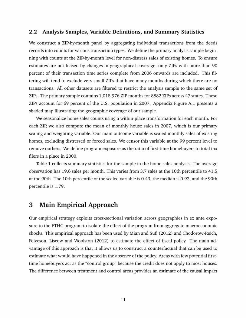
2.2 Analysis Samples, Variable Definitions, and Summary Statistics

We construct a ZIP-by-month panel by aggregating individual transactions from the deeds

records into counts for various transaction types. We define the primary analysis sample begin-

ning with counts at the ZIP-by-month level for non-distress sales of existing homes. To ensure

estimates are not biased by changes in geographical coverage, only ZIPs with more than 90

percent of their transaction time series complete from 2006 onwards are included. This fil-

tering will tend to exclude very small ZIPs that have many months during which there are no

transactions. All other datasets are filtered to restrict the analysis sample to the same set of

ZIPs. The primary sample contains 1,018,976 ZIP-months for 8882 ZIPs across 47 states. These

ZIPs account for 69 percent of the U.S. population in 2007. Appendix Figure A.1 presents a

shaded map illustrating the geographic coverage of our sample.

We seasonalize home sales counts using a within-place transformation for each month. For

each ZIP, we also compute the mean of monthly house sales in 2007, which is our primary

scaling and weighting variable. Our main outcome variable is scaled monthly sales of existing

homes, excluding distressed or forced sales. We censor this variable at the 99 percent level to

remove outliers. We define program exposure as the ratio of first-time homebuyers to total tax

filers in a place in 2000.

Table 1 collects summary statistics for the sample in the home sales analysis. The average

observation has 19.6 sales per month. This varies from 3.7 sales at the 10th percentile to 41.5

at the 90th. The 10th percentile of the scaled variable is 0.43, the median is 0.92, and the 90th

percentile is 1.79.

3 Main Empirical Approach

Our empirical strategy exploits cross-sectional variation across geographies in ex ante expo-

sure to the FTHC program to isolate the effect of the program from aggregate macroeconomic

shocks. This empirical approach has been used by Mian and Sufi (2012) and Chodorow-Reich,

Feiveson, Liscow and Woolston (2012) to estimate the effect of fiscal policy. The main ad-

vantage of this approach is that it allows us to construct a counterfactual that can be used to

estimate what would have happened in the absence of the policy. Areas with few potential first-

time homebuyers act as the “control group” because the credit does not apply to most houses.

The difference between treatment and control areas provides an estimate of the causal impact

11

of the program.10

We measure exposure to the FTHC by identifying places with more first-time buyers in a

time period prior to the policy. Higher exposure likely reflects local amenities, such as schools

or social attractions, that attract first-time buyers. Or it may reflect a local housing stock

that is better suited to these buyers, in terms of affordability, lot size, and so on. The policy

primarily targeted first-time homebuyers, so we should expect larger impact in places where

historically first-time homebuyers are more likely to buy. We build the exposure measure at the

ZIP level because we are interested in the effect of the policy on market-level outcomes such

as house prices. These local general equilibrium or market effects would be missed if we used

a household-level identification strategy.

This approach permits an estimate of the aggregate effect of the program under various

assumptions we consider about the macroelasticity as a function of exposure. We primarily as-

sume this elasticity is a constant function of exposure, though we also estimate heterogeneous

effects in robustness tests. Our approach does not naturally map into a person-level microe-

lasticity of housing demand with respect to the program. To explore the latter, we consider a

complementary regression kink research design that exploits the program’s income eligibility

threshold. Section 4.5 describes this design in more detail.

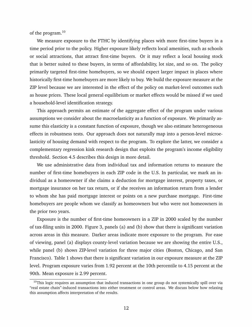
We use administrative data from individual tax and information returns to measure the

number of first-time homebuyers in each ZIP code in the U.S. In particular, we mark an in-

dividual as a homeowner if she claims a deduction for mortgage interest, property taxes, or

mortgage insurance on her tax return, or if she receives an information return from a lender

to whom she has paid mortgage interest or points on a new purchase mortgage. First-time

homebuyers are people whom we classify as homeowners but who were not homeowners in

the prior two years.

Exposure is the number of first-time homeowners in a ZIP in 2000 scaled by the number

of tax-filing units in 2000. Figure 3, panels (a) and (b) show that there is significant variation

across areas in this measure. Darker areas indicate more exposure to the program. For ease

of viewing, panel (a) displays county-level variation because we are showing the entire U.S.,

while panel (b) shows ZIP-level variation for three major cities (Boston, Chicago, and San

Francisco). Table 1 shows that there is significant variation in our exposure measure at the ZIP

level. Program exposure varies from 1.92 percent at the 10th percentile to 4.15 percent at the

90th. Mean exposure is 2.99 percent.

10This logic requires an assumption that induced transactions in one group do not systemically spill over via“real estate chain”-induced transactions into either treatment or control areas. We discuss below how relaxingthis assumption affects interpretation of the results.

12

Consistent with anecdotal accounts of where first-time homebuyers tend to buy, exposure

is relatively concentrated in suburban areas around cities. Table 2 confirms this with a set of

bivariate regressions of program exposure on ZIP-level observables. ZIPs with high exposure

have higher rents and fewer people below the poverty line. The populations are larger and

somewhat younger. Income is weakly correlated with program exposure. Substantial variation

in ex ante exposure within cities allows us to pursue a research design that conditions on city-

by-time fixed effects.11

Our measure may not accurately capture exposure to the program, either because the tax

data miss non-filing or non-itemizing households, or because places change over time. To

address this concern, we show that places with higher ex ante exposure indeed saw more

individuals claim the credit. We do so in two ways. Figure 4, panel (a) plots binned bivariate

averages (“binscatters”) of FTHC claims from tax records versus program exposure. Exposure

is strongly correlated with take-up in the cross section. The regression coefficient with CBSA

fixed effects and ZIP-level covariate controls is 0.59 with a clustered t-statistic of 20.

Figure 4, panels (b) and (c) show our exposure measure also predicts time series varia-

tion in claims in these areas. We plot counts of FTHC claims by month of home purchase for

purchases made between February 2009 and September 2010 along with vertical markers for

policy events. The vertical markers correspond to the start of the FTHC loan program, the start

of version two of the credit, the scheduled expiration of version two, and the actual expiration

of version three, respectively. Panel (b) plots national claim counts month-by-month, while

panel (c) plots claim counts for high- and low-exposure quintiles of ZIP codes sorted by ex

ante exposure.12 Not only does our exposure measure predict that high exposure places claim

more credits, but the measure also predicts the spikes in claims that we observe in the national

claims data. We conduct a number of robustness tests to confirm these results do not depend

on the precise way in which we measure exposure. Consistent with exposure being a slow-

moving characteristic of places, Appendix Figure A.4 shows that exposure is highly correlated

over time and that alternative measures of exposure yield nearly identical take-up predictions.

While our measure is strongly correlated with FTHC take-up, a concern is that unobservable

characteristics unrelated to the FTHC program are responsible for any differential purchase

patterns we observe. Table 2 shows that places where first-time homebuyers typically buy are

not random, which poses a potential challenge to our empirical approach. For example, a

risk to our design is that our measure captures the expansion in subprime credit documented

11We use Core-Based Statistical Areas (CBSA) to define city boundaries. Though exposure varies at the ZIPlevel, we cluster standard errors at the CBSA level to permit within-city correlation in error terms.

12Quintiles are formed using weights that ensure each quintile has equal population in 2007.

13

by Mian and Sufi (2009), leading to different ZIP-by-time trends within cities as the cycle

corrected. To mitigate this risk, our preferred measure is the number of first-time homebuyers

in a pre-subprime period, the year 2000, which ensures the exposure measure is not driven by

increased purchases by subprime borrowers later in the decade.13 We also control directly in

our empirical analysis for the subprime share of borrowers in 1996 (Mian and Sufi’s (2009)

measure) and the subprime share of loans in 2004–2007.

We employ multiple additional strategies to mitigate concerns about differential ZIP-by-

time trends. First, our baseline analysis always conditions on city-by-time fixed effects and we

report results with and without observable controls. This approach removes many potential

confounds from our analysis. Second, we explicitly test for parallel trends in the pre-period,

perform within-ZIP placebo tests, explore heterogeneous effects by credit generosity, and con-

trol for contemporaneous housing market policies to further assess this concern. Third, we

exploit information in the age distribution of first-time homebuyers over time, showing that

the median age of first-time homeowners falls during the policy period and the age distribu-

tion reverts immediately after the policy expires. Moreover, the highest exposure ZIPs account

for the largest share of the shift in first-time homebuyer age observed in the aggregate data.

Finally, we exploit the short-lived nature of the policy to argue against potential alternative sto-

ries. In particular, the sharp increase in housing sales before the expiration of both the second

and third versions of the program is difficult to explain by confounding trends that operate at

lower frequencies.

4 The Effect of FTHC on Home Sales and Homeownership

4.1 Home Sales

We begin with a simple graphical analysis that demonstrates our main finding: home sales

respond strongly to the FTHC program but do not show a sharp, immediate reversal once the

program ends.

Figure 5, panel (a) plots the monthly home sales series between July 2007 and September

2011 for ZIPs divided into 100 quantiles and sorted based on ex ante program exposure. We

present these data in the form of a calendar time heatmap, which is analogous to the traditional

13The year 2000 is the earliest year for which at least one year of information returns from lenders are availableto classify past homeownership. Appendix Tables A.5 and A.6 show our results do not depend on the year in whichwe measure exposure due to its high persistence over time. Because place-based exposure is persistent over time,choosing an early year does not fully address the subprime concern. Examining pre-trends is therefore key forevaluating the role of confounding factors.

14

two-group calendar time graph but allows us to plot visually discernible time series for many

more groups. In the graph, columns correspond to months and rows correspond to groups of

ZIPs sorted by exposure. Each cell’s shading corresponds to a level of the key outcome variable,

which is monthly home sales scaled by average monthly home sales in 2007. The quantiles are

formed using weights that ensure each quantile has an equal number of home sales in 2007.

The heatmap yields four conclusions. First, high- and low-exposure series closely track

each other every month prior to the policy, deviating only during the policy window. Note

that every sequence of consecutive months in the pre-period provides a placebo test that fails

to reject the design’s core identification assumption of parallel trends. Second, the smoothly

increasing gradient visible at each policy expiration date shows the policy response is monotone

in ex ante exposure and not driven by a few outlier ZIP codes. Third, the gradient does not

reverse significantly in the fifteen months following the second policy expiration, rather the

series return to a pattern of parallel trends; thus the data do not indicate a sharp reversal

of the policy response. Last, we will use the lowest exposure quantile as a counterfactual to

estimate the cumulative number of sales induced by the program. The heatmap shows that

this group is a credible counterfactual, as it indicates no response to the program during the

policy period.

Figure 5, panel (b) plots coefficients from regressions estimating the monthly effects of the

program. Specifically, we run month-by-month regressions of the form,

Home Salesi

Average Monthly Salesi,2007

= αCBSA + βExposurei + γX i + εi, (1)

where Exposurei is the geographic measure of program exposure for place i and αCBSA is a

CBSA-specific constant.14 In controls specifications, X i is a control set that includes log pop-

ulation, the average unemployment rate from 2006 through 2010, log average gross income

in 2005, the subprime share in 1996, the average share of subprime originations from 2004

to 2007, exposure to the 2009 FHA expansion, and exposure to the HARP and HAMP pro-

grams. All regressions are weighted by average monthly home sales in 2007. Note that this

approach is approximately equivalent to a panel regression with time-specific coefficients on

exposure and the control variables and with ZIP, month, and CBSA-by-month fixed effects.15

14For the 129 ZIPs without an associated CBSA, we assign them a state-specific constant.15This cross sectional approach closely matches the approach taken by Mian and Sufi (2012) to evaluate the

Cash for Clunkers program, which aids comparison to their findings. We have also pursued the more stan-dard difference-in-differences approach in a panel regression, as advocated by Bertrand, Duflo and Mullainathan(2004) and pursued in Best and Kleven (2017). Figure 5, panel (d) and Appendix Table A.1 present estimatesbased on this approach, which yields very similar results.

15

To aid interpretation, we normalize exposure by its cross sectional standard deviation.

Panel (b) plots coefficients for these regressions with controls. The patterns are consistent

with those in the heatmap. Exposure patterns do not predict differences in sales activity until

the policy window begins and the coefficients spike in accord with the aggregate series. The co-

efficient of 0.05 for November 2009 implies that a one standard deviation increase in program

exposure produces a 5 percent increase in monthly home sales relative to the average level in

2007. This is approximately 0.12 standard deviations of the left hand side variable. Panel (c)

plots coefficients for regressions which replace monthly sales with cumulative monthly sales

beginning seventeen months prior to the policy. The series is approximately flat prior to the

policy window, increases monotonically through the window, and flattens in the post period.

The cumulative effects are between 50 and 60 percent relative to the average level of monthly

sales in 2007. Note these should not be confused for aggregate estimates, which we provide

below. Again, we see no evidence of a sharp, negative relationship between sales and exposure

in the seventeen months following the policy. At longer horizons—between a year and quarter

and three years after the policy expired—our cumulative regressions begin to lose statistical

power because each subsequent month of home sales adds noise and increases standard errors.

Still, we can reject at the 95 percent level a full reversal through 2012.

Panel (d) plots coefficients from a panel specification. We estimate a regression at the ZIP

level from 2004 onward, weighted by total home sales in 2007, of the form,

log(Home Sales)i t = αi +δCBSA,t +∑

t

βtExposurei +∑

t

γt X i + εi t ,

in which βt is a month-specific exposure coefficient and γt is a vector of month-specific co-

efficients on ZIP-level controls. We plot coefficients on exposure from January 2006 onward,

omitting January 2004 through December 2005. Coefficients in this specification closely match

those in panel (b), both in pattern over time and magnitude.

Table 3 presents the average monthly effects of the FTHC on home sales pooled over dif-

ferent policy windows for a variety of specifications. We run cross sectional regressions of the

form,Average Monthly Salesi,t→T

Average Monthly Salesi,2007

= αCBSA + βExposurei + γX i + εi, (2)

where the left hand side numerator is average monthly home sales in place i over the relevant

time period. We use the same control set, weighting, and specification for exposure as in Figure

5, panels (b) and (c). Standard errors are clustered at the CBSA level, or for ZIPs that are not

associated with a CBSA, at the state level. Note that each row reports estimates from a separate

16

cross sectional regression.

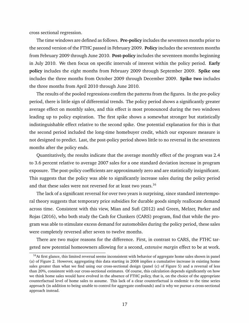
The time windows are defined as follows. Pre-policy includes the seventeen months prior to

the second version of the FTHC passed in February 2009. Policy includes the seventeen months

from February 2009 through June 2010. Post-policy includes the seventeen months beginning

in July 2010. We then focus on specific intervals of interest within the policy period. Early

policy includes the eight months from February 2009 through September 2009. Spike one

includes the three months from October 2009 through December 2009. Spike two includes

the three months from April 2010 through June 2010.

The results of the pooled regressions confirm the patterns from the figures. In the pre-policy

period, there is little sign of differential trends. The policy period shows a significantly greater

average effect on monthly sales, and this effect is most pronounced during the two windows

leading up to policy expiration. The first spike shows a somewhat stronger but statistically

indistinguishable effect relative to the second spike. One potential explanation for this is that

the second period included the long-time homebuyer credit, which our exposure measure is

not designed to predict. Last, the post-policy period shows little to no reversal in the seventeen

months after the policy ends.

Quantitatively, the results indicate that the average monthly effect of the program was 2.4

to 3.6 percent relative to average 2007 sales for a one standard deviation increase in program

exposure. The post-policy coefficients are approximately zero and are statistically insignificant.

This suggests that the policy was able to significantly increase sales during the policy period

and that these sales were not reversed for at least two years.16

The lack of a significant reversal for over two years is surprising, since standard intertempo-

ral theory suggests that temporary price subsidies for durable goods simply reallocate demand

across time. Consistent with this view, Mian and Sufi (2012) and Green, Melzer, Parker and

Rojas (2016), who both study the Cash for Clunkers (CARS) program, find that while the pro-

gram was able to stimulate excess demand for automobiles during the policy period, these sales

were completely reversed after seven to twelve months.

There are two major reasons for the difference. First, in contrast to CARS, the FTHC tar-

geted new potential homeowners allowing for a second, extensive margin effect to be at work.

16At first glance, this limited reversal seems inconsistent with behavior of aggregate home sales shown in panel(a) of Figure 2. However, aggregating this data starting in 2008 implies a cumulative increase in existing homesales greater than what we find using our cross-sectional design (panel (c) of Figure 5) and a reversal of lessthan 20%, consistent with our cross-sectional estimates. Of course, this calculation depends significantly on howwe think home sales would have evolved in the absence of FTHC policy, that is, on the choice of the appropriatecounterfactual level of home sales to assume. This lack of a clear counterfactual is endemic to the time seriesapproach (in addition to being unable to control for aggregate confounds) and is why we pursue a cross-sectionalapproach instead.

17

These are home purchases that would not have taken place absent the FTHC. Consistent with

our results, Best and Kleven (2017) study a similar policy in the U.K. and find that the exten-

sive margin can be large in the short run. Second, the long duration of the policy relative to

CARS and the ability to pair the credit with a low down payment loan (discussed further in

Section 5.3) meant that FTHC brought durables demand from much farther in the future than

the CARS program, potentially causing a slower reversal. In a follow-up paper (Berger, Cui,

Turner and Zwick, 2017), we use an estimated structural model to explore the quantitative

magnitudes of these two effects, as well as how policy design can affect the relative size of the

intertemporal and the extensive margin effects.

4.2 Robustness and Placebo Tests

Table 3 presents a number of tests to confirm the robustness of our key findings, including the

absence of trends prior to the policy, the effect estimates during the policy period, the estimates

at the two spikes, and the non-reversal in the post-policy window.

Column (1) estimates the specification in equation (2) without CBSA fixed effects and con-

trols. Column (2) adds a control set that includes log population, the average unemployment

rate from 2006 through 2010, log average gross income in 2005, the subprime share in 1996,

the average share of subprime originations from 2004 to 2007, exposure to the 2009 FHA ex-

pansion, and exposure to the HARP and HAMP programs. Column (3) adds CBSA fixed effects.

Columns (3) through (5) all use the same control set as column (2) and all include CBSA fixed

effects. Estimates are similar with and without CBSA fixed effects, though somewhat more

precise in the former specification.

In our main specification, we weight regressions by average monthly home sales in 2007

in order to provide macroeconomically relevant estimates. Column (4) presents regressions

without weights. Unweighted regressions lead to modestly larger estimates during the policy

window. Regressions with population weights, which we do not report for brevity, lead to

similar conclusions. Following Mian and Sufi (2012), column (5) excludes the sand states:

Arizona, California, and Nevada. Excluding sand states only slightly weakens the size of policy

period estimates. In general, estimates are very similar across states.17

Importantly, the parallel trends assumption test yields coefficients close to zero across spec-

17Appendix Table A.1 replicates the baseline results and these robustness checks using a log specification basedon Best and Kleven (2017). The table also considers an alternative pre period that separates version one of theFTHC program (i.e., the Loan Program spanning 2008m5 to 2008m12) and the two years prior to version one.The table suggests modest effects of version one, approximately one-third the size on a monthly basis and 16percent on a cumulative basis relative to versions two and three (i.e., the Grant Program).

18

ifications, and we find similarly null average post-policy effects. Appendix Figure A.2 presents

a placebo test that further confirms these findings. The test estimates the month-by-month

regressions and plots coefficients from the non-control specification in Figure 5, panel (b), em-

phasized with a bold line, along with equivalent regressions shifted backward in time to start

in 2005, 2006, and 2007, and shifted forward to start in 2009 and 2010. These placebo series

show that the policy coefficients are unusually high while pre- and post-policy coefficients co-

incide with placebo series. The figure also suggests that seasonal confounds not captured by

our seasonality adjustment do not influence our estimates for the spikes.

The pre-policy coefficients provide strong evidence that our design is valid and low ex-

posure areas can serve as a counterfactual to high exposure areas. The sharp timing of the

policy addresses many concerns about omitted variables because most potential confounds

are moving more slowly. Yet some concerns might remain. One concern is that time-varying,

place-specific shocks are correlated with our exposure measure. For example, suppose our

exposure measure is highly correlated with the share of subprime borrowers, which peaked

during the years from 2004 to 2007. If true then the increase in sales we witness during the

policy period could be driven by “pent-up” subprime demand and not the causal effect of the

FTHC. While the inclusion of CBSA-by-month fixed effects helps mitigate these concerns, there

is still significant variation in subprime borrowing within CBSAs. However, Table 2 shows that

our exposure measure is essentially uncorrelated with the share of subprime borrowers—using

both Mian and Sufi’s (2009) subprime measure and a measure of subprime borrowing from

2004 to 2007—suggesting that our main results are not driven by a subprime, pent-up demand

effect.

An additional concern is that place-specific trends beginning in 2009 might confound our

estimates. Such trends could be driven by coincident policies designed to shore up the housing

market or by place-specific cyclicality. We address this threat in three additional ways.

First, we construct controls designed to capture the exposure of ZIP codes to different hous-

ing market programs. The most relevant coincident program is the expansion of the FHA loan

limits in 2009, which persisted in the years following the FTHC program. We measure expo-

sure to this FHA policy change using the average share of loan originations in HMDA data in

2004–2007 that would have been eligible under the new regime. Appendix Figure A.5 shows

this measure strongly predicts FHA take-up at the ZIP level, but is weakly negatively correlated

with FTHC exposure (the correlation of -0.04 is reported in Table 2). Because the FHA policy

change targeted larger mortgages, it affected buyers in higher price local areas that are gen-

erally too expensive for first-time homebuyers. We also follow Agarwal, Amromin, Ben-David,

19

Chomsisengphet, Piskorski and Seru (2017) and Agarwal, Amromin, Chomsisengphet, Pisko-

rski, Seru and Yao (2017) to construct measures of exposure to the HARP and HAMP programs,

which attempted to alleviate debt burdens among underwater borrowers. For HARP, we use

the ZIP-level share of loan originations purchased by Fannie Mae or Freddie Mac over 2004 to

2007. For HAMP, we use an estimate of the ZIP-level share of mortgage modifications under

the HAMP program. Table 2 shows that these programs also targeted different areas than the

FTHC program, as correlations are close to zero. We include exposure measures for each of

these programs in our control set, though weak correlations imply our estimates do not depend

on these controls.

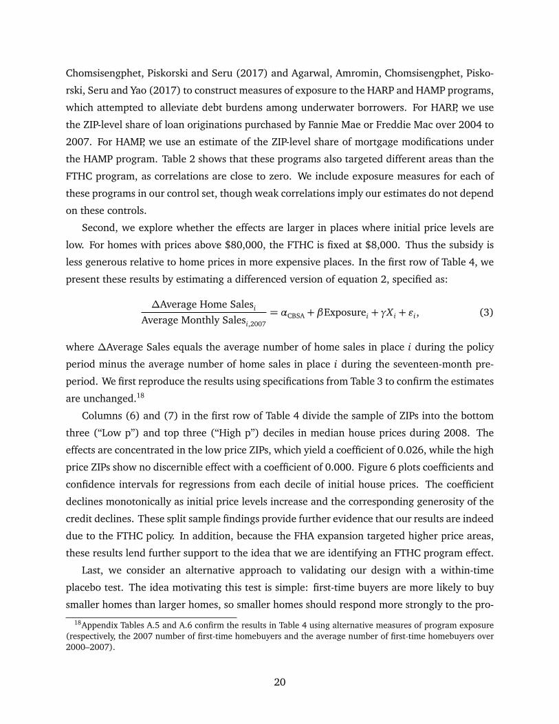
Second, we explore whether the effects are larger in places where initial price levels are

low. For homes with prices above $80,000, the FTHC is fixed at $8,000. Thus the subsidy is

less generous relative to home prices in more expensive places. In the first row of Table 4, we

present these results by estimating a differenced version of equation 2, specified as:

∆Average Home Salesi

Average Monthly Salesi,2007

= αCBSA + βExposurei + γX i + εi, (3)

where ∆Average Sales equals the average number of home sales in place i during the policy

period minus the average number of home sales in place i during the seventeen-month pre-

period. We first reproduce the results using specifications from Table 3 to confirm the estimates

are unchanged.18

Columns (6) and (7) in the first row of Table 4 divide the sample of ZIPs into the bottom

three (“Low p”) and top three (“High p”) deciles in median house prices during 2008. The

effects are concentrated in the low price ZIPs, which yield a coefficient of 0.026, while the high

price ZIPs show no discernible effect with a coefficient of 0.000. Figure 6 plots coefficients and

confidence intervals for regressions from each decile of initial house prices. The coefficient

declines monotonically as initial price levels increase and the corresponding generosity of the

credit declines. These split sample findings provide further evidence that our results are indeed

due to the FTHC policy. In addition, because the FHA expansion targeted higher price areas,

these results lend further support to the idea that we are identifying an FTHC program effect.

Last, we consider an alternative approach to validating our design with a within-time

placebo test. The idea motivating this test is simple: first-time buyers are more likely to buy

smaller homes than larger homes, so smaller homes should respond more strongly to the pro-

18Appendix Tables A.5 and A.6 confirm the results in Table 4 using alternative measures of program exposure(respectively, the 2007 number of first-time homebuyers and the average number of first-time homebuyers over2000–2007).

20

gram. If ZIP-level shocks are driving our results, we should see similar patterns across all types

of homes. Appendix Table A.3 presents regressions of the same form as those in Table 3. We di-

vide the home sales series into “starter” homes—defined as those with 1, 2, or 3 bedrooms—and

large homes—defined as those with 4 or more bedrooms. We run the ZIP-level specifications

separately for each series.19 Estimates for the starter home sample closely match those in our

full sample, while those for larger homes are weakly negative and statistically insignificant.

Thus, our main results are concentrated among starter homes, while larger homes show little

response to the program.

4.3 The Age Distribution of First-Time Buyers

The non-reversal of the policy period response following the program’s expiration raises the

question of where these buyers came from. To address this question, Figure 7 presents direct

evidence indicating that, in the absence of the program, many buyers would not have bought

homes for several years. Panel (a) plots age distributions of first-time homebuyers identified

using information return data for the years between 2002 and 2013. We highlight the age

distribution for 2009, which shifts substantially to the left relative to the other years. The years

from 2002 through 2008 (long dashed lines) reveal an age distribution that is considerably

older than the 2009 cohort. In the four post-policy years from 2010 to 2013 (short dashed

lines), the age distribution closely resembles the pre-policy years, though with more mass in

the early and mid 30s and less mass between 40 and 50. The median age for all first-time

buyers is 35 in the non-policy years and 33 in 2009. Among those that claimed the credit, the

median was 32.

To confirm the FTHC explains this pattern, panel (b) shows the correlation between the

shift in the age distribution in 2009 and program exposure. We decompose the national shift

in the age distribution in 2009 into contributions from each ZIP. For each ZIP, we compute the

difference between the ratio of buyers aged 30 or younger to total new homebuyers in 2009

versus the average ratio of buyers aged 30 or younger to total new homebuyers in other years.

We then plot binned bivariate sums of these ZIP-level contributions against average exposure

in each bin. The highest exposure ZIP codes account for the largest share of the shift in first-

time homebuyer age observed in the aggregate data. Thus a noticeably younger cohort of

first-time buyers appears in 2009 alone, driven by the temporary policy incentive to accelerate

the transition into homeownership.

19Because of incomplete reporting across places, the analysis sample here is the subset of the main analysissample where fewer than 5% of transactions between 2004 and 2013 have missing bedrooms data.

21

These facts also assuage concerns that place-by-time cyclicality, pent-up demand, or secu-

lar trends can explain the slow reversal. For example, since many first-time homebuyers buy

with FHA-insured loans, the expansion of FHA’s loan limits in 2009 might interfere with our

empirical approach. However, such a confound would predict the shift in the age distribu-

tion of first-time homebuyers to continue in the years after the FTHC expired, contrary to the

temporary shift in the age distribution we see in the data.

4.4 New Construction

Our analysis thus far has focused on non-distress sales of existing homes. This is the largest

category of transactions and is the most reliably recorded in the DataQuick database. Both of

these features permit the high-frequency analysis we use to validate our research design. Yet

in examining the policy as fiscal stimulus intended to spur GDP growth, existing home sales

are not the ideal category to study, as they only contribute to output through transaction fees

and complementary purchases (such as furniture) made by homeowners.

In Table 4, we explore the effects of the program on new home sales, using the new con-

struction data recorded by DataQuick. To do so, we estimate a differenced version of equation

2, specified as

∆Average Constructioni

Average Monthly New Constructioni,2007

= αCBSA + βExposurei + γX i + εi, (4)

where ∆Average Construction equals the average number of new home sales in place i during

the policy period minus the average number of new home sales in place i during the seventeen-

month pre-period. We seasonally adjust the new home sales series prior to averaging. All

specifications include CBSA fixed effects.

The results indicate the program had approximately no effect on new home sales. The point

estimate is -0.002 and not statistically distinct from zero, as compared to 0.021 for existing

home sales. We confirm this finding in several robustness checks. Column (2) equally weights

observations and column (3) excludes the sand states: Arizona, California, and Nevada. Columns

(4) and (5) confirm that the results are not driven by outliers or small geographies. Column

(4) estimates the relationship on a subsample that censors the left-hand-side variable at the

5th and 95th percentiles. Column (5) restricts the sample to places with average home sales

in 2007 above the 10th percentile.

All specifications point to the conclusion that FTHC did not induce additional construc-

tion. This finding is not surprising for a time when the national market suffered a significant

22

overhang of recently built homes and elevated vacancies. Nevertheless, the result implies that

the FTHC’s direct stimulative effects through residential investment were likely second order,

despite the substantial increase in existing home sales caused by the program.

4.5 Homeownership

To supplement our earlier findings on the effect of the FTHC on home sales we provide evi-

dence from a regression kink design (RKD). This approach allows us to both characterize the

aggregate effect of the FTHC during the first year of the policy period and estimate the un-

derlying response at the individual level. To implement the RKD, we draw on administrative

population-level tax data and exploit the phase-out range of the FTHC.

Background and data. The maximum value of the FTHC is $8,000 but it phases out for

higher income taxpayers. In 2009, joint taxpayers with adjusted gross income (AGI) less than

$150,000 were eligible for the maximum credit. The FTHC linearly phased out over the next

$20,000, so that joint taxpayers with an AGI at $170,000 or above were not eligible for the

credit. Among single taxpayers in 2009, those with AGI less than $75,000 were eligible for the

maximum, and thus the credit was completely phased out by $95,000.20

We refer to the point where the FTHC begins to phase out as the “kink point” because the

value of the FTHC has a kink, or slope change, at this point. As a result, taxpayers with AGI

below the kink can receive the maximum credit while taxpayers with AGI above the kink point

are eligible for a smaller credit. The RKD exploits this kink point by relating the slope change

in the FTHC to the slope change in the likelihood of being a first-time homebuyer.

To construct our sample we draw on population-level administrative tax data. These data

have two key advantages for the RKD research design. First, they provide a large sample size

close to the kink point: our baseline sample includes over 3.8 million observations. A second

advantage of the data is that they provide an accurate measure of income, so that measurement

error in the distance to the kink point and exposure to the FTHC is negligible.

We draw samples within +/-$8,000 of the kink point, located at $75,000 for single tax-

payers and $150,000 for joint taxpayers. We define first-time homebuyers as those who pay

mortgage interest in 2009, but where the primary taxpayer (and secondary taxpayer among

joint taxpayers) have not paid interest in the prior three years.

20In 2010, the phase-out points increased to $125,000 for single taxpayers and $225,000 for joint taxpayers.We find no evidence that the credit increased homeownership at these higher income levels using an RKD. Becauseof smaller sample sizes, however, the estimates are not precise enough to exclude the estimates from the 2009kink.

23

Method. To identify the causal effect of the FTHC on the likelihood of being a first-time

homebuyer, we use a “sharp” RKD. We estimate the intention-to-treat effect, as we impute the

value of the FTHC for all observations and relate the slope change of this potential FTHC to the

slope change in the probability of being a first-time homebuyer. The causal effect of the FTHC

on being a first-time homebuyer is the ratio of the slope change in the probability of being a

first-time homebuyer and the slope change in the potential FTHC.

Following prior work (Card, Lee, Pei and Weber, 2015; Nielsen, Sørensen and Taber, 2010;

Manoli and Turner, 2018), we focus on a constant effect additive model to examine the effect

of the FTHC on homeownership at the household level:

First-Time Homebuyeri = βFTHCi + g(Kink Distancei) + εi,

where First-Time Homebuyeri is an indicator equal to one if the household is a first-time home-

buyer, FTHCi is the value of the credit in hundreds of nominal dollars, and kink distance is the

distance in hundreds of nominal dollars to the kink point. The function g is a continuous func-

tion of kink distance, and the FTHC is assumed to be a continuous and deterministic function

of kink distance with a slope change at 0. The average treatment effect is given by:

β =limk→0+

∂ E[First-Time Homebuyeri |Kink Distancei=k]∂ k |k=0 − limk→0−

∂ E[First-Time Homebuyeri |Kink Distancei=k]∂ k |k=0

limk→0+∂ E[FTHC|Kink Distancei=k]

∂ k |k=0 − limk→0−∂ E[FTHC|Kink Distancei=k]

∂ k |k=0

.

The numerator of this expression is the slope change around the kink in the probability of being

a first-time homebuyer. The denominator is the slope change around the kink of the FTHC. We

estimate the numerator with a regression of the form:

First-Time Homebuyeri = γKink Distancei +δDiKink Distancei +πX i + νi, (5)

where Di is an indicator equal to one if the tax return has AGI above the kink point, X i is a

vector of covariates including controls for AGI, ZIP code, and indicators for age and number of

dependent children. The sharp RKD uses the statutory slope change so that the RKD estimator

is given by β = δ−0.4 , where −0.4 is the statutory slope change in the FTHC at the kink point.21

When estimating the regression in (5), we use a bandwidth of +/-$8,000. This bandwidth

allows us to control for a nonlinear relationship between income and homeownership that is

separate from the slope change at the kink point. We can separate income from kink distance

because of the simultaneous existence of two kinks, one for single and one for joint filers. We

21The FTHC is reduced from $8,000 to $0 over a $20,000 interval of AGI, giving a slope of -0.4.

24

also use these kinks to conduct placebo tests by placing filer groups at the alternative kink. We

conduct further placebo tests using non-policy years.

Results. Figure 8 presents results and robustness checks in graphical form. In each graph,

we pool both single and joint filers after recentering their AGI relative to their respective kinks

and plot binned means for 50 equal-density bins.

Panel (a) plots the statutory kink for those who claim the credit, revealing the sharp kink

induced by the phase-out region. The average level of credit to the left is slightly below $8,000

because some claimants are restricted by the purchase price of the house or apartment they

buy. Panel (b) plots the reduced form effect of the FTHC, revealing a kink in the propensity of

homeownership that closely matches the kink location in the FTHC schedule.

Table 5 presents estimates of the reduced form effect, which correspond to the paramater

δ in equation (5). Given low baseline first-time homebuyer rates, we multiply the estimates

by 105 for ease of readability. Standard errors are clustered at the ZIP code level to account

for geographic covariance in the error term. Appendix Table A.4 reports summary statistics

for the estimation sample. Columns (1) through (6) present regressions that vary the control

set, which includes a linear control for AGI, a three-knot cubic spline in AGI, ZIP code fixed

effects, primary taxpayer age fixed effects, and number of children fixed effects. The controls

have essentially no effect on the estimated kink, which varies from -3.7 to -4.0 with t-statistics

between 6 and 7.

We conduct three additional tests to confirm the robustness of this result. First, Figure 8,

panel (c) plots predicted first-time homeowner rates as a function of income, age fixed effects,

ZIP code fixed effects, and number of children fixed effects. This figure tests the continuity and

smoothness of the underlying densities of these covariates, which are necessary for the validity

of the RKD. The predicted homeownership rates show no kink at the statutory kink.

Second, Figure 8, panel (d) plots reduced form plots for all years from 2005 through 2013.

The figure serves as a visualization of an RK difference-in-differences design, in which the non-

kink years 2005 through 2008 and 2010 through 2013 provide placebo tests. As the housing

cycle evolves, the average first-time homebuyer rate falls and recovers. Yet only in 2009 do we

observe the pronounced kink in the propensity to buy coinciding with the statutory kink. The

figure rules out most alternative explanations for the observed kink in 2009.

The third robustness check is a within-2009 placebo test. We divide the sample into single

and joint filers in 2009 and estimate placebo kinks for single filers at the joint filer kink and

vice versa. Table 5, columns (7) and (8) present the single filer estimates, and columns (9) and

25

(10) present the joint filer estimates. For both groups, we find sharp and precise estimates at

the true statutory kink and no evidence of a similar kink at the placebo. In summary, we find

strong evidence of a causal effect of the FTHC on the home purchase decision at the individual

level, which is unlikely to be driven by confounding factors.

Our preferred estimate of -3.8×10−5 for $100 in kink distance implies the effect of the

full $8000 of FTHC causes an increase in first-time homebuyer propensity by 0.76(= (−3.8×10−5)/(−0.4)·(80)) percentage points. This effect raises the within-sample baseline rate of 1.43

percentage points by 53 percent, an economically large effect. As is standard in discontinuity

designs, such an estimate relies on extrapolation of the local treatment effect identified around

the kink to larger changes in the credit amount. However, the local effect is identified under

quite weak assumptions (DiNardo and Lee, 2011). We also report a separate estimate that

restricts the treatment population to those filers who are eligible for the FTHC because they

were not homeowners in the prior three years. Table 5, column (11) reports this estimate,

which equals -1.6×10−4 or an effect of 3.2% for the full credit (relative to a baseline rate

of 5.4%). While not the primary focus of this paper, this microelasticity with respect to the

credit is of independent interest for considering the microeconomic effects of housing market

subsidies.

5 The Effect of FTHC on Reallocation

Traditional policy evaluations focus on the direct stimulative effects of fiscal policy. In this

section, we move beyond the standard view and consider the value of the program as a housing

market stabilizer. Consistent with the aim of mitigating fire sale spillovers, we find the FTHC

increased house prices and induced significant reallocation of assets from distressed sellers to

high-value buyers.

The backdrop of the policy was a time of extraordinary weakness in housing markets across

the country. Inventories were at historic highs and nearly forty percent of home sales were

distressed or foreclosure sales. Many prospective homebuyers were financially constrained,

making it difficult to afford required down payments. When combined with high numbers of

unsold homes, this drag on housing demand put significant downward pressure on housing

prices. Against this backdrop came widespread concern that absent government intervention,

fire sale dynamics would continue, leading to more vacancies and foreclosures, more destruc-

tion of housing wealth, and further downward pressure on prices.22

22Consistent with this view, Mian, Sufi and Trebbi (2015) provide empirical evidence that foreclosures led to a

26

These economic conditions created several rationales for stabilizing the housing market,

of which we highlight three. The first is to address the pecuniary externality that elevated

foreclosures, short sales, and vacancies impose on nearby homeowners. Campbell, Giglio and

Pathak (2011) show that prices for houses within 0.05 miles of a foreclosure fall by about one

percent. Similarly, Whitaker and Fitzpatrick IV (2013) find that an additional property within

500 feet that is vacant or delinquent reduces a home’s selling price by 1 to 2 percent. Guren

and McQuade (2015) show that these effects can be large in a quantitative, general equilibrium

model. Policies that stabilize house prices during a period of market-level distress can mitigate

this market failure.

A second rationale is to correct a credit market failure due to the simultaneous presence

of constrained buyers and elevated vacancies. In normal times, buyers purchase homes until

the marginal cost and marginal benefit of homeownership equate. During the Great Recession

a wedge between these margins emerged: many natural buyers of homes were constrained

because of elevated unemployment risk, lower incomes, and disruptions in the credit market.

Because the vacant homes had already been built, the marginal cost of delivering a house was

lower than the marginal benefit to a household of living there. The fact that vacant homes

depreciate faster due to lack of maintenance (Gerardi, Rosenblatt, Willen and Yao, 2015) and

may enable crime (Ellen, Lacoe and Sharygin, 2013; Cui and Walsh, 2015) further strengthens

the case. A policy like the FTHC—which alleviates credit constraints faced by new homebuyers

and may move people into underutilized homes—could improve welfare.

Finally, a large literature documents how a decline in house prices can affect the real econ-

omy via balance sheet effects. Falling house prices generate financial accelerator effects by

destroying household net worth and thus affecting whether firms can borrow to invest and

whether households can borrow to consume (Kiyotaki and Moore, 1997; Iacoviello, 2005).

These effects would be particularly strong during a liquidity trap, as was the case during the

FTHC program. There is considerable evidence that these effects were large: falling house

prices led to a large decline in consumption and employment during the Great Recession (Mian

and Sufi, 2011, 2014). Housing prices can also affect the balance sheets of banks and an in-

crease in foreclosures can spill over to the banking sector as losses realized by banks inhibit

their ability to borrow and lend (Shleifer and Vishny, 2010b). A policy which increased housing

prices would have recapitalized households, firms, and banks.

Taken together, these rationales provide a justification for attempting to stabilize house

prices. In the next section, we present evidence suggesting the additional demand induced by

large decline in house prices, residential investment, and consumer demand during the Great Recession.

27

the FTHC program indeed increased house prices and facilitated a productive reallocation of

underutilized assets. We make this case in three steps. First, we evaluate the effect of the FTHC

on house prices. Consistent with a reallocation toward higher utility users, we find the program

increased house prices significantly: in our preferred specification, a one standard deviation in

exposure to the program caused the median home to appreciate by $2,390. Second, we show

that many transactions during the policy period involved sales by investors and institutional

sellers, who were likely to be low utility users of the assets or involved highly motivated sellers

whose homes were in foreclosure and thus likely in financial distress. Third, many buyers

induced by the program were likely constrained by down payment requirements that the credit

and concurrent federal lending policies helped relax. In addition, a large fraction of purchased

homes were previously vacant or were foreclosures, consistent with positive reallocation and

improved utilization of existing assets. Finally, we find the marginal reallocation caused by the

program was stable, as program buyers were not more likely to default than other cohorts and

the quantity and price responses reversed slowly and partially.

5.1 House Prices

To explore the effect of the FTHC on house prices, we use data from the Federal Housing

Finance Agency (FHFA), CoreLogic, and DataQuick. The first two datasets rely on a repeat

sales methodology to estimate price indices at the ZIP level from the present to as far back as

the mid 1970s. The FHFA indices use all mortgages guaranteed by Fannie Mae and Freddie

Mac, and offer the greatest geographic coverage but are only estimated annually. CoreLogic’s

index uses its proprietary database to estimate monthly values. We augment this analysis by

using micro-data from DataQuick to explore the effect of the policy using raw, transaction-level

prices.

We follow the same empirical strategy as for the home sales regressions in Table 4, exploit-

ing within-CBSA variation in exposure to the program. For the FHFA data, the left-hand-side

variable is cumulative annual log price differences during 2009 and 2010 minus cumulative

annual log price differences during 2007 and 2008. We use a long-difference specification be-

cause unlike housing transactions, which are well measured, month-to-month changes in house

price indices, especially at the ZIP level, are quite noisy. We present estimates for raw changes

in price growth and for market-adjusted changes. In the case of market-adjusted changes, we

first estimate ZIP-specific housing market betas in the ten-year window from 1997 to 2006 and

then subtract beta times the market return to compute a ZIP-level excess return.23 This allows

23For the market return, we use the national annual FHFA house price index, which is estimated using a similar

28

us to control for differential exposure of high exposure ZIP codes to the national cycle driven

by higher risk in these areas. For the CoreLogic data, the left-hand-side variable is raw cumu-

lative monthly log price differences during the policy period minus cumulative monthly log

price differences during the 17-month pre-period. In all cases, we multiply the left-hand-side

by 100 so the treatment effect units are percentage points of growth per standard deviation

change in program exposure.

Table 6 presents results from these regressions. In our preferred specification, which uses

the market-adjusted FHFA series, we find the program caused an increase in cumulative price

growth of 1.077% per standard deviation increase in exposure. At the median initial price level

of $222,000 in our sample, this implies an increase in prices of $2,390 (≈ .01077 × 222,000).

This figure is plausible given the $8,000 size of the credit and considerable excess inventory

in the market. It also implies that even the highest exposure places did not see house prices

increase by more than the credit.24

As shown in the table, the estimate is robust to different weights, sample definitions, and

censoring of the left-hand-side variable. In addition, the estimates vary little between the FHFA

and CoreLogic samples and do not depend on the market adjustment for ZIP-specific cyclicality.

As with the quantity results, we estimate more precise and qualitatively larger effects in the

ZIPs with lower initial house prices, though these differences are only statistically significant

in the CoreLogic sample.

Figure 9 allows us to explore the extent to which the price effects reverse in the years

following the policy. We estimate cross-sectional regressions each year of first differences in

market-adjusted price growth from the FHFA. The coefficients show no pre-trends in years

prior to the program and strong trend breaks during the two program years, which match

both qualitatively and quantitatively the positive long difference effects estimated in Table

6. In the year immediately following the program, price growth retreats somewhat, undoing

approximately one quarter of the increase caused by the program. This evidence is consistent

with an incomplete reversal of the home sales response in the post-policy period.

Our micro-level estimates provide strong cross-sectional evidence that the FTHC increased

house prices. While these results are informative about the effectiveness of the FTHC policy,

their value in enabling a welfare analysis is incomplete because the research design removes

macro variation from the estimates. As a result, there is no necessary connection between the

micro-level results and the effect of the program on aggregate house prices: it is possible for

methodology to the ZIP-level indices.24As house prices were falling on average during this time, these effects may be interpreted as saying the

program slowed the rate of price declines.

29

strong micro-level and weak macro-level effects to coincide. Thus, despite obvious limitations,

examining aggregate house price data is useful for gaining insight into whether the FTHC

succeeded at stabilizing the aggregate housing market.

Figure 10, panel (a) plots the monthly CoreLogic national house price index (thick gray

line) and three separate price indexes we build from DataQuick transaction data for the period

between 2004 and 2013. The CoreLogic index is based on repeat sales pairs and incorporates a

three-month moving average to smooth the aggregate data. The raw repeat index (dotted blue

line) follows published methodology from CoreLogic and S&P Case-Shiller for including sales

pairs and estimating price indices. The moving average repeat index (thin red line) applies a

three-month moving average to the raw repeat index. The raw mean price index (dashed black

line) includes all transactions, winsorized at the one percent level to reduce the influence of

outliers.

At first glance, there appears to be mixed evidence that the FTHC affected aggregate house

prices. All four series show a precipitous decline in prices starting in 2007, which slows dra-

matically in the first quarter of 2009, consistent with a positive policy effect. The CoreLogic

index shows two humps in price levels that appear to lag the credit’s expiration dates. However,

there is little evidence in any of the three repeat sale price indices that prices appreciated con-

siderably during the policy period. In contrast, the raw aggregate price index, which includes

every transaction, suggests significantly greater price appreciation during the policy period and

persistent effects after the policy expires. What explains the difference?

Relative to raw prices, the repeat-sales indices make several adjustments in estimation

and sample selection, the effects of which are illustrated by our replication. These adjust-

ments include applying a 3-month lagged moving average smoother to the estimated series

and down-weighting transaction pairs with higher predicted variance of price changes. Our

moving average replication matches CoreLogic closely, but the raw repeat-sales index shows

bumps in prices that more closely coincide with the spikes in aggregate transactions. In addi-

tion, the repeat-sales index excludes transactions for which the reference property only sells

once during the estimation period, and the most commonly cited repeat-sales indices exclude

multifamily units and condominiums (including our CoreLogic series and replication).

Taken together, these adjustments will tend to obscure the effect of the program on ag-

gregate prices, either by smoothing sharp changes in the time series or through excluding

transactions that are more likely to be bought by first-time homebuyers or to see significant

price increases during this time. Figure 10, panels (b) and (c) show that only using repeat

transactions to construct the price index is a significant restriction. This restriction excludes

30

just under half of total arms-length transactions on average, with a bias toward recently built

homes. Importantly, these excluded transactions are not missing at random over time: during

the policy period, the share of excluded transactions closely mirrors the time series pattern of

aggregate sales shown in Figure 2. Many of the housing transactions that were induced by the

policy are being excluded from the price index, potentially biasing downward our estimated

price effects. The fourth row of Table 6 confirms these suspicions. Estimated price effects in

the raw data are approximately twice the size of our baseline specifications. However, these

estimates are noisier due to the small set of transactions that drive ZIP-level means and we

cannot reject the hypothesis that the price effects are the same in raw prices and using price

indices. Nevertheless, we conclude the price effects of the program are likely obscured by the

metholodogy of standard price indices.

We have presented both micro- and macro-level evidence demonstrating that the FTHC

was successful at both stimulating housing transactions and raising house prices. These facts

are consistent with the idea of policy-induced beneficial reallocation from low-value sellers to

high-value buyers. An alternative story is that the FTHC worked because it heavily subsidized

homebuyers and lured low-value buyers into the market. The fact that house prices increased

is our first piece of evidence against this alternative interpretation.

5.2 Recently Built Homes and Homes in Distress

We exploit the richness of the DataQuick transaction data, which records the names of buyers

and sellers as well as categories for distressed sales, to explore how likely it was that the FTHC

sped reallocation of houses from low- to high-utility users. For each property, DataQuick’s

county assessor data provide detailed information on the characteristics of the transacted

homes, including price, size, age and number of bedrooms and bathrooms. Linked to each

property are transaction data that track changes in deed. The data identifies if a transaction is

a short sale, a financial institution-owned sale (REO), a foreclosure auction, or an exchange of

deed on a foreclosed home. DataQuick’s proprietary model classifies whether the transaction

is made between related parties or at arm’s length.

It is important to distinguish sellers who are homeowners from those left holding assets

they were unable to sell. A number of negative externalities are associated with the latter case.

Empty houses decay more rapidly and can be subject to vandalism or host to other crimes.

Foreclosure spillovers associated with forced sales of distressed homes can depress housing

values for neighbors and, through subsequent reappraisals, amplify barriers to refinancing.

We divide the total transactions for our main analysis sample during the policy period into

31

categories based on the likelihood that the sellers were not first-best users of the homes they

were selling. We investigate the following categories:25

1. Recently Built: Includes homes built between 2005 and 2010.

2. Short Sale: Includes homes categorized by DataQuick as short sales (i.e., sales involvingprincipal forgiveness by lenders).

3. Foreclosure/Real Estate Owned (REO): Includes homes categorized by DataQuick asbeing sold from a financial institution’s portfolio of homes or through a foreclosure auc-tion.

4. Developer Seller: Includes homes for which the seller is either a home builder or otherkind of company, based on the seller’s name.

5. Government Sponsored Enterprise (GSE) Seller: Includes homes for which the selleris a federal entity—Fannie Mae, Freddie Mac, Ginnie Mae, the Federal Home Loan Banks,or the Veterans Administration.

During the policy period, there were 4.3 million total transactions in our sample. Approx-

imately 739 thousand of those were homes that had been built in 2005 or later. This com-

pares to 396 thousand homes classified as new construction by DataQuick. To the extent our

new construction marker is too restrictive, these sales indicate the program may have allowed

builders to sell homes from their recent inventories. Consistent with this, approximately 1.13

million homes, or 24 percent of all home sales, were sold by developers or builders. Thus

nearly two-thirds of homes sold by developers were not new construction.

Recent construction does not contribute to output or employment at the time of sale. How-

ever, the importance of recent construction in aggregate sales during this period highlights

two macroeconomic issues created by investment overhangs. First, an overhang of previously

built assets reduces investment today while the economy redeploys excess inventory. Second,

while GDP correctly measures the delivery of new homes during the period of construction, it

does not correctly measure the initiation of a stream of consumption services if those assets are

subsequently left vacant. The facts suggest programs like the FTHC can work by accelerating

redeployment and initiating use of idle assets.

Distressed sales and sales from financial institution portfolios were also important during

this time. Within our sample, there were approximately 561 thousand short sales and 843

thousand foreclosure or REO sales, including 235 thousand sales from the government entities’

portfolios of repossessed homes. While not mutually exclusive from the recent construction

25Appendix A provides more detail on how we categorize transactions, including regular expressions used toidentify builders, developers, and the GSEs.

32

and developer sales above, these figures again suggest that many of the homes transacted

did not involve transfers from one homeowner to another, but instead enabled transitions of

underutilized assets to more productive use.

In the last row of Table 4, we focus on foreclosures and short sales and use program expo-

sure to study the effect of the program on distressed sales. As with non-distressed sales and new

construction, we estimate a differenced version of equation 2, where the left-hand-side variable

is the average number of foreclosures and short sales in place i during the policy period mi-

nus the average number of foreclosures and short sales in place i during the seventeen-month

pre-period, scaled by the average in 2007. We seasonally adjust the distressed sales series

prior to averaging. All specifications include CBSA fixed effects. The point estimate is 0.037

and marginally statistically significant in some specifications. The magnitude suggests the pro-

gram induced a modest shift in the composition of sales toward distressed sales. Columns (2)

through (7) confirm the robustness of this finding, as do specifications in Appendix Tables A.5

and A.6 with alternative exposure measures. Note that this effect is in addition to the effect on

distressed transactions due to the increase in the level of demand caused by the program.

5.3 Constrained Buyers and Mortgage Finance

A large literature documents the importance of down payment constraints in housing markets.

Stein (1995) shows that modeling down payment constraints is crucial for matching many

empirical features of the housing market. Using the PSID, Engelhardt (1996) shows that young

households reduce consumption in years in which they buy a home and increase consumption

back to long-run levels in subsequent years. This suggests that the down payment constraint

is binding for many young households. Survey evidence confirms this fact. Fuster and Zafar

(2015) administer a survey on the role of down payment constraints on household willingness

and ability to buy housing. They find that a reduction in down payments would have a much

larger effect on household behavior than a decline in mortgage rates. This result reflects the

difficulty many households face in saving for the typical 20 percent down payment, especially

in high home price areas.26

The FTHC program coincided with an expansion by the Federal Housing Administration

(FHA) of its first-time homebuyer mortgage guarantee program. This program enables mort-

gage loans of up to 96.5 percent of purchase price for eligible buyers. Given the low down

26A report by builderonline.com finds that residents making the median income in a state have to save nearlyeight years on average to put 10 percent down for a median price home (builderonline, 2015). Similarly, a surveyby Trulia.com finds that a full 47 percent of surveyed renters would consider buying if they had enough savingsfor the down payment (Kolko, 2012).

33

payment requirements, first-time homebuyers make up a significant portion of new origina-

tions supported by the FHA, as the government-sponsored enterprises Fannie Mae and Freddie

Mac typically require larger down payments. According to the Department of Housing and

Urban Development (HUD), FHA supported 781 thousand first-time homebuyers during 2009

and 882 thousand during 2010, or approximately 56 percent of the first-time buyer market

during these years.27

These low down payment loans are not costless: a lower upfront payment trades for higher

subsequent interest payments plus required mortgage insurance premiums. A simple calcula-

tion highlights the trade-off. Consider three different mortgage contracts for a house which

costs $200,000: (1) a conventional 30-year fixed rate mortgage requiring a 20 percent down

payment, (2) a 96.5 percent loan-to-value (LTV) FHA loan where the household pays off the

Upfront Mortgage Insurance (UMI), 1.75 percent of price, within the down payment, (3) a

96.5 percent LTV FHA loan that shifts the UMI into the principal. The FHA loan also includes a

0.55 percent mortgage insurance premium. Assume the interest rate is 4.8 percent, the average

conventional mortgage rate from November 2009.28

Under these assumptions and no discounting, the first mortgage would cost $301,000 over

30 years. Notice that to receive this contract the buyer makes a $40,000 down payment at

origination. The second mortgage would cost $368,000 over 30 years but the buyer would

only make a $7,000 + $3,500 down payment upfront. Finally, the third mortgage including

UMI would cost about $375,000 over 30 years and the buyer would make a $7,000 down

payment. In 2009, the average interest rate on FHA loans was 1.4% higher than a conventional

mortgage, which increases the cost of the FHA loans to $428,500 and $436,000 respectively.

Thus the FHA mortgages are considerably more expensive over the life of the contract than a

conventional mortgage. That so many households chose an FHA mortgage despite the higher

future cost suggests that down payment constraints were highly relevant for these households

during the sample period.29

Part of the FHA expansion came from increased loan limits through the FHA Forward pro-

gram initiated as part of the Economic Stimulus Act of 2008. This contemporaneous policy

raises concern that we incorrectly attribute effects of the FHA policy change to the FTHC pro-

gram. However, Appendix Figure A.5 shows that areas targeted by this policy were higher price

areas not particularly exposed to the FTHC. As noted above, controlling for ZIP level exposure

27See Figure 6 in HUD’s “Annual Report to Congress” (Department of Housing and Urban Development, 2011).28For the sake of simplicity we abstract from mortgage prepayment and exclude the tax benefits of interest

payments and insurance premiums.29Conversations with economists at the Department of Housing and Urban Development confirm that borrowers

were permitted to apply the credit toward the 3.5 percent down payment.

34

to the FHA policy change does not alter our estimates. Thus, the more relevant part of the

FHA expansion for our purposes came through loans that qualified under the pre-crisis regime.

This expansion occurred as the private market for second liens to reduce down payments con-

tracted.30

A final piece of evidence of binding constraints comes from the patterns of FTHC claims

via amended tax returns. By amending a prior return, buyers could accelerate the credit’s

payment to the time of purchase, instead of waiting until filing the next year’s return. For

most buyers, waiting until next year’s return meant receiving the credit in May or June of

2010, potentially a year after purchase. The data reveal that the majority of buyers strongly

preferred to receive their credit immediately, as 53 percent of claims came via amended returns.

In addition, this share is decreasing in age. Among buyers aged 30 or younger, the amended

share is 57 percent. In contrast, only 48 percent of buyers aged 40 and older claimed the credit

via amended return. These patterns suggest immediate liquidity demands, which are typically

higher for young households, were very important to FTHC claimers.

The data strongly suggest that many potential homebuyers face down payment constraints,

as these buyers took advantage of low down payment loans at the expense of higher monthly

payments. The FTHC program helped relax these constraints; as a result, many marginal trans-

actions likely involved purchases by high-value users of the assets. When combined with the

facts about home sellers, this further suggests that induced sales entailed productive realloca-

tion.

5.4 Vacant Homes and Household Formation

To further assess the likelihood of beneficial reallocation, we complement our exploration of

low-utility sellers from Section 5.2 with information from the de-identified tax returns of FTHC

claimers. Unfortunately, the tax data do not record information about the people or entities

from whom FTHC claimers bought their homes. Nor can we use aggregate data to asset this

question since the effect of housing demand on aggregate vacancies is ambiguous.31 However,

it is possible to use information about mailing addresses to ask two related questions about

claimer transitions into homeownership. The first question is whether the home occupied by

the claimer at the time of purchase was occupied in recent years or instead a vacant home.30See HUD Mortgagee Letter 2009-07 and Goodman, Seidman and Zhu (2014) for more detail on the FHA loan

limit expansion. A distinct mortgage assistance program called FHA Secure, created in August 2007 and expandedin July 2008, is also unlikely to bias our results, as this program only enrolled a few thousand borrowers.

31While an increase in the demand for housing lowers vacancies, all things equal, an increase in expectationsof future housing demand could lead to an increase in vacancies if more current homeowners choose to list theirhome.

35

The second question is whether the transition induced household formation in the sense that

claimers move from a multiple occupancy household to a single occupancy household.

We attempt to measure vacancy and household formation using mailing address informa-

tion reported on an individual’s tax return.32 To measure changes in vacancy status, we ask

whether the new address associated with the FTHC purchase had been occupied two years

prior to the purchase. To measure changes in household formation, we count the number of

tax returns filed from a particular address and compare it to the number of tax returns filed

at the FTHC claimer’s address two years prior to the purchase. In both cases, we choose the

period two years prior because the new address may be assigned to the prior year’s tax return if

a tax filer amended the prior return to claim the credit. We focus on claims made for purchases

in 2009 to separate first-time homebuyers from long-time homebuyers.

From the FTHC claims in 2009, we find that 42 percent move into an address that had no

filers in 2007 and 33 percent transition into a single tax filer address from living in a multiple

filer address in 2007.33 We have also computed these statistics for first-time homebuyers in the

non-policy years between 2002 and 2013. The data suggest that FTHC claimers are not more

likely to move into vacant homes, but are more likely to form new households relative to first-

time buyers in other years (33.1% transition to single family in 2009 relative to 30.5% in other

years). In years prior to the crisis, high vacancy rates may instead reflect new construction.

We assess this issue by dividing first-time homebuyer addresses based on whether the address

appears in previous years. Using this method, on average 13.9% of these addresses between

2002 and 2007 can be classified as new construction. In 2009, only 7.9% of addresses can be

classified this way, lending further support to the notion that FTHC buyers were often buying

recently vacated homes.

Taken altogether, to the extent the program sped reallocation of underutilized assets, this

reallocation came primarily through increasing the level of home purchases during a time

when the supply of vacant homes was abnormally high. Nevertheless, the data do rule out

the possibility that FTHC purchases merely resulted in people “swapping” houses. In addition,

the data also suggest imputed owner-equivalent rental income as another indirect GDP effect

of the program.

32Specifically, we use the mailable point information encoded in the 12-digit ZIP code. We restrict analysis tovalid ZIP-12s, i.e., ZIP-12s where the last seven digits are not all zeros.

33The household formation statistic restricts the sample to those filers for whom we have a valid previousaddress. As a validation check of the vacancy data, we have confirmed that the vacancy share of FTHC claims atthe ZIP level is strongly correlated with the share of home sales that are foreclosures or short sales.

36

5.5 Default Rates for Policy Period Buyers

Given the high origination loan-to-value ratios of policy period homebuyers and the literature

suggesting such LTVs can lead to distress, it is critical to ask what happened to these buyers

subsequently. We use the DataQuick transaction data to shed light on this question. DataQuick

records track a distressed property as it goes through each step of the default process, as early

as a short sale and as late as the REO disposal following foreclosure. We use chronological

changes in ownership classified as distress sales by DataQuick to identify homebuyers who later

defaulted on their loan. Specifically, we follow policy period cohorts of buyers and compare

them to cohorts both before and after the policy. We restrict analysis to buyers with FHA-

insured mortgages in order to focus on those with high potential default risk.

Figure 11, panel (b) plots cumulative distress cohorts for purchases made during the policy

period and compares these to cohorts based on 2006, 2007, and 2008 sales as well as cohorts

based on 2011 sales. Our data allow us to compare cohorts for at least 36 months from the

month of purchase. Both the 2009 and 2010 policy cohorts show no difference in default

rates relative to the 2011 post-policy cohort. At 36 months out, each of these groups shows

distress transition rates of approximately ten per thousand purchases. Furthermore, all three

of these groups display considerably lower rates of transition into distressed sales than the

pre-policy groups. Thus the data do not indicate the FTHC program induced unusually risky

buyers into the market, despite the very high LTVs at which these buyers entered. In this sense,

the reallocation of homes appears to have been stable.

6 The Aggregate Effect of the FTHC

6.1 Aggregate Effect on Home Sales

An important motivation for the FTHC policy was to stimulate real economic activity, particu-

larly in the housing sector. For new home sales, the effect is the value of the homes exchanged;

however, we have shown that this effect was likely small for the FTHC. For existing home sales,

the effect is through complementary purchases and transaction fees. To estimate this effect,

we first construct an estimate of the total number of existing sales caused by the program. We

compute this estimate using three different methodologies based on our alternative research

designs. Reassuringly, all three approaches yield similar results.

37

Method 1: Cross-sectional approach. Following Mian and Sufi (2012), we start by comput-

ing an estimate of the total number of sales caused by the program, exploiting only differences

in cross sectional exposure and using the group receiving the smallest shock as a counterfac-

tual. We choose the bottom one percent of ZIPs as the counterfactual group, which corresponds

to the bottom row of the heatmap in Figure 5, panel (a). We then compute the effect of the

policy for other groups relative to this group. By construction, any time series effect of the

policy shown by the bottom group is set to zero and removed from the effect computed for

other groups.

Standardized exposure is 0.85 for the bottom group and increases to 7.58 for the highest

group. Thus for each exposure group g, the aggregate number of sales induced by the program

is

∆Salesg = 17× β × (eg − 0.85)× sg,2007, (6)

where β is the coefficient from equation (2) for the seventeen-month policy period, eg and

sg,2007 are weighted average program exposure and monthly sales in 2007 for group g, respec-

tively, where the weights are average monthly sales for the ZIPs in each group. We aggregate

∆Salesg across all groups to provide an estimate of the aggregate effect within the DataQuick

sample.

We estimate that the FTHC increased existing home sales by 169,000 within sample during

the policy period, or 8.1 percent of all sales during this period. In 2007, our sample covers

approximately 41 percent of the national existing home sales market. Extrapolating our esti-

mates to the national market yields an estimated increase of approximately 412,000 during the

policy period. There were 2.74 million claims of the FTHC during this time with a total outlay

of $20.3B.34 Thus, under the assumptions that the lowest exposure group is a plausible control

group and that our sample is representative of the national market, 15 percent of claims were

made for induced sales, as opposed to sales that would have happened in the absence of the

policy. Note this is a lower bound estimate if the lowest exposure group also responds to the

program. A less conservative approach, which aggregates estimates relative to a zero exposure

baseline, yields an estimate of 233,000 within sample, or 11.2 percent of all sales during the

policy period. The extrapolated aggregate estimate in this case is 568,000 and implies that 21

percent of claims were made for induced sales. The implied direct fiscal costs based on these

two approaches are approximately $49K and $36K per induced sale, respectively.35

34This figure excludes approximately 550,000 claims for the Long-Time Homebuyer Credit.35Our primary specification is a reduced form regression of sales on exposure, and so delivers an intention-to-

treat (ITT) estimate. Two-stage estimates with total claims per filing unit as the endogenous first stage variableyield a first stage coefficient, β1S = 0.568(0.048), and a policy period second stage coefficient, βIV = 5.26(1.72).

38

To produce this aggregate estimate, we have not modeled potential general equilibrium

effects, which are subsumed into time fixed effects. In response to the concern about general

equilibrium effects, it is comforting that the raw aggregate path of home sales provides a clear

demonstration of a policy response. Furthermore, the heatmap does not reveal home sales

falling below pre-policy levels in low exposure areas, which would be predicted by binding

aggregate resource constraints. In addition, because the policy was implemented at a time

when interest rates were at the zero lower bound, the mitigating effect of interest rates was

likely small. Nevertheless, without a full model, our aggregate estimate should be considered

an imperfect approximation of the total effect.

An additional concern is that spillovers between the treatment and control ZIPs might bias

our aggregate calculation. This could happen if a housing purchase in a high-exposure ZIP

triggers a simultaneous purchase by the previous seller in a low exposure ZIP. Two features of

our analysis suggest these “real estate chain”-induced spillovers are likely not quantitatively

important. First, the inclusion of CBSA fixed effects means that only transactions that take

place within the same city would bias our estimates. Second, many sellers during this time

period were either banks or developers, cases in which these spillover effects are not relevant.

Finally and most importantly, the most plausible sign of the bias is negative since the second

transaction would artificially inflate sales in the lower exposure ZIPs. Thus our aggregate

estimates are likely an underestimate of the true aggregate effect.

Method 2: Regression kink (RK) approach. We can also obtain an estimate of the total size

of the FTHC program using the micro-level estimates from our RK design. Our preferred spec-

ification implies the full FTHC credit increased the first-time homebuyer propensity by 0.76%

among all tax filers and 3.2% among eligible tax filers. We use these individual elasticities to

generate an estimate of the aggregate effect of the policy.

The aggregate estimates are given by 0.76% times the number of tax filers in 2009 with

incomes below the phase-out (69 million), and 3.2% times the number of eligible tax filers in

2009 (19 million). These estimates imply 520,000 or 610,000 households, respectively, were

induced by the FTHC to purchase homes. Though using a different source of identification,

these estimates are quite close to the range implied by our cross-sectional approach, lending

further credibility to each research design.

This coefficient implies a one standard deviation change in claims (0.018) causes an increase of scaled sales of0.095; alternatively, this estimate implies 0.15 sales per claim, consistent with our aggregate calculation. As thisestimate corrects for noncompliance with treatment, aggregating the policy effect using this estimate and a ZIPcode sort based on claims yields a larger aggregate estimate: approximately 242,000 within sample. We focus onthe reduced form estimate for ease of interpretation.

39

Method 3: Age distribution approach. We obtain an alternative estimate of the aggregate

effect of the FTHC program using variation embedded in the age distribution of first-time buy-

ers, which shifts substantially towards young buyers in 2009. We use this variation to construct

our third estimate, which focuses on the total number of young buyers caused by the program.

We first divide the age distribution in 2009 into a young group of those under 35 and a

benchmark group of those above 35. We then use the years 2002 through 2007 to estimate

the average density in the young group with a simple regression of group shares on age bins.

This regression yields a counterfactual predicted density, f youngt 6=2009, and a predicted counterfac-

tual number of young buyers according to the formula, f youngt 6=2009 = N young

2009,c f /(Nyoung2009,c f +Nnot young

2009 ).

The estimate of induced young buyers is the difference between actual young buyers and coun-

terfactual buyers.

Under the assumption that older buyers are unaffected by the program, this procedure

yields an aggregate estimate of 261,000 induced buyers under 35, or approximately 22% of

first-time buyers in this age group identified in our data. This estimate provides a lower bound

on the overall estimate as the assumption that older buyers are unaffected is too strong. Nev-

ertheless, the age distribution research design provides an alternative source of variation that

complements our main design and yields a similar estimate at the group level.

6.2 Direct Stimulative Effects

We now provide a back-of-the-envelope calculation of the direct fiscal multiplier using our

aggregate estimates of induced home sales. As in Best and Kleven (2017), we abstract from

any dynamic effects, thus our estimates are best interpreted as a lower bound since any post-

policy reversal would lower them.36

We first consider the income generated for realtors. On average, the realtor fee ranges

from 5 to 5.5 percent of the purchase price.37 When evaluated at the median purchase price

for homes in our sample during the policy period ($190,000), this implies a lower and upper

bound on the GDP contribution of $3.9 and $6.4 billion, respectively.38

Next, we draw on Best and Kleven (2017) and Benmelech, Guren and Melzer (2017), who

36We choose to focus on the static effects for three reasons. First, given that we argue that the direct stimulativeeffects are modest, this assumption is conservative. Second, this assumption has no bearing on our second point,which is that the indirect effects are larger than the direct effects because it affects both proportionately. Third,assuming no reversal is a useful benchmark given that we find little evidence of reversal even two years after theFTHC ended.

37Based on data collected by the Department of Justice at https://www.justice.gov/atr/home-prices-and-commissions-over-time (last accessed in August, 2016).

38$3.9 billion = 0.05×190K×412K; $6.4 billion = 0.055×190K×610K.

40

estimate that complementary furniture, home improvement, and related expenditures at the

time of a new purchase amount to approximately 1.9–2.8 percent of the purchase price. Using

our aggregate estimates, this implies an additional contribution to GDP between $1.5 billion

and $3.2 billion.39 Combining these two calculations, the overall direct contribution to GDP

of the FTHC was between $5.4 and $9.6 billion, significantly less than the $20.3 billion cost

of versions two and three of the program. These estimates imply the FTHC generated impact

fiscal multipliers between 0.27 and 0.47, much smaller than the typical tax multiplier during

recessions. Altogether, these calculations lead us to conclude that the that the direct GDP

effects of the program were relatively modest and significantly below its overall cost.40

6.3 Indirect Stimulative Effects

Section 5 presented evidence that the FTHC played an important role in stabilizing housing

markets in the aftermath of the Great Recession. One of the main channels through which the

policy did so was by increasing home values: a one standard deviation increase in program

exposure caused the median home to appreciate by approximately $2,390. Given that the

FTHC had a significant effect on house prices, natural questions to ask are: first, did the FTHC

indirectly stimulate consumption for both claimers and existing homeowners through its effect

on house prices, and second, how large are these effects?

A recent and growing empirical literature documents large, causal responses of non-durable

consumption to house price movements. Using different identification strategies, these studies

estimate an elasticity of non-durable consumption in the range of 0.15 to 0.3.41 Because house

price appreciation affects existing homeowners, it is possible these indirect effects are large, as

housing wealth is the largest component of net worth for most households.42

In order to derive a ballpark estimate of this effect, we apply the rule-of-thumb formula in

Berger, Guerrieri, Lorenzoni and Vavra (2017) to our empirical setting. The central theoretical

result of Berger, Guerrieri, Lorenzoni and Vavra (2017) is that despite the many ways in which

a change in house prices affects an individual’s decision problem, the change in consumption

39$1.5 billion = 0.019×190K×412K; $3.2 billion = 0.028×190K×610K.40Best and Kleven (2017) find that the stimulative effect of temporary changes in transaction taxes are much

larger than ours: their estimates suggest that the impact multiplier is around 2. One potential difference is theirpolicy variation affects all buyers, including repeat buyers who may be more elastic than new homebuyers.

41See, e.g., Mian, Rao and Sufi (2013), Stroebel and Vavra (2016), and Kaplan, Mitman and Violante (2016).42A separate question is whether the credit itself affected the consumption of claimers. We focus on the response

of consumption to an equilibrium change in house prices rather than this direct effect of receiving the creditbecause (a) the former effect is likely larger and (b) the direct effect is ambiguous. If the credit does not affectthe size of home purchased, the direct consumption effect could be large due to the cash transfer to households.If buyers adjust their home purchase size, direct consumption effects would be smaller.

41

due to an unexpected, proportional change in house prices is given by a simple rule-of-thumb

formula:∆Ci∆PP

= M PCi · (PHi−1(1−δ)), (7)

where M PCi is the individual marginal propensity to consume out of transitory income shocks

and PHi−1(1− δ) is the value of the individual’s home after depreciation. Given estimates of

these objects, we can aggregate them across households and places and evaluate the size of

the indirect effects under a variety of assumptions.

We proceed as in Section 6.2 by choosing the bottom one percent of ZIPs as the counter-

factual group and computing an aggregate house price effect for other groups relative to this

group. Recall that the standardized exposure is 0.85 for the bottom centile and increases to

7.58 for the highest one. Thus for each exposure group g, the aggregate percentage change in

prices for that group induced by the program is

∆Pg

Pg= βp × (eg − eg,low) (8)

where βp is the coefficient (0.01077) from the long difference price regression in Table 6. We

apply this price growth factor to the average median house price in each group and accumulate

over all owner-occupied housing units in each group under an assumed value for the marginal

propensity to consume. We then apply equation (7) to infer the aggregate change in consump-

tion induced by the policy. These calculations are rough but informative for the magnitude of

potential indirect effects.

If one assumes that the MPC is 0.10 and all of the housing stock is affected, then aggregate

consumption would have increased by $27 billion on account of the FTHC.43 If one assumes

instead that only one- to three-bedroom homes are affected by the policy, the effect is approx-

imately $15 billion. This exercise is too coarse to permit emphasis of a particular number; the

key takeaway is that these effects can be as large or possibly much larger than the program’s

direct stimulative effects: even our conservative estimate implies a multiplier for the indirect

effect of 0.74, considerably larger than the direct effect. Combining both effects yields a total

impact fiscal multiplier of the FTHC policy between 1.01 and 1.8, most of which comes from

the indirect effect—the component typically ignored in most policy evaluations.

43This MPC is an average of estimates from the fiscal transfer literature (0.2-0.3) and the value implied by thepermanent income hypothesis (0.05), similar to the estimates in Di Maggio, Kermani, Keys, Piskorski, Ramcharan,Seru and Yao (2017).

42

7 Conclusion

This paper asks whether policy can accelerate the process of reallocation in times of debt-

induced capital overhang following an investment boom. We study temporary tax incentives

targeted at marginal asset buyers in the housing market. Unlike debt renegotiation programs,

financial market support, and fiscal and monetary stimulus, the policy we study directly tar-

geted the capital overhang, while aiming to keep underused assets in private hands.

The program proved effective at spurring home sales, and these effects did not immediately

reverse once the program ended. While the research design does not permit us to say whether

there is a permanent component to the increase in home sales, we can conclude these sales

were not reversed for at least two years. This stable demand shock to the market accelerated

the process of reallocation of vacant homes from institutional investors, banks, and the unsold

inventories of home builders into the hands of higher value users. House prices increased and

buyers induced by the program were not more likely to default than previous or subsequent

cohorts of buyers. These results suggest correctly targeted policies can accelerate purchases

and mitigate the debt-deflation dynamics associated with capital overhang.

The FTHC policy also stimulated homeownership. This is notable because the U.S. gov-

ernment spends at least $70 billion a year on the mortgage interest deduction, partly to en-

courage homeownership. While the mortgage interest deduction may have some effect on

inducing marginal households into homeownership, it also induces households already plan-

ning to buy a home into buying larger homes, which has limited social benefits (Glaeser and

Shapiro, 2003; Kirker, Floetotto and Stroebel, 2016). One lesson from the FTHC is that, if

increasing homeownership rates is a policy goal, then directly targeting potential homeowners

and the constraints they face may be a more cost-effective way to achieve this goal. Of course

our paper does not speak adequately to this comparison of policies. More research into the

question should be pursued.

Since the increase in housing transactions came largely in the existing home market, the

policy is less appealing when considered as fiscal stimulus. While resales do increase GDP

through increased realtor fees and complementary purchases, the effect on GDP was likely

below the cost of the program, even accounting for high aggregate spending multipliers due

to the zero lower bound.

Given this evidence, was the FTHC a successful policy? The evidence is mixed. If judged

solely on its direct stimulative impact, the policy would receive a low mark. Taking a wider

view of the policy—as a housing market stabilizer during a time of extreme distress in the

housing market—leads to a more generous appraisal. By inducing constrained renters to buy

43

earlier in their life cycle, the policy prevented inefficient liquidation of housing and preserved

housing wealth.44 The policy enabled beneficial reallocation of unoccupied housing stock to-

ward higher value users and stabilized house prices. This made the FTHC complementary to

other principal and payment renegotiation programs, such as HAMP and HARP, that aimed to

repair household balance sheets and improve mortgage affordability. The key difference is that

the FTHC addresses a later stage in the foreclosure chain, namely, when the house is already

owned by the bank.

Recent theoretical work on macro stabilization policy when there is capital overhang is

consistent with this appraisal. Proposition 2 in Rognlie, Shleifer and Simsek (2014) shows

that in a model with aggregate demand externalities, policies like the FTHC are optimal if

the amount of capital overhang is large enough.45 Hedlund (2016) writes a housing search

model where government interventions in the housing market can improve welfare, especially

for highly levered agents, if they lower liquidity frictions allowing constrained househoulds

to better insure themselves against negative income shocks by more easily accessing trapped

housing wealth.46 The combination of a deep recession and significant capital overhang is

crucial to both results.

Thus, policies like the FTHC may prove useful in the policy toolkit for helping the economy

recover from fire sales associated with debt-induced capital overhang. Nonetheless, in order

for government intervention to be justified it must be the case that the falling prices induced

by the fire sale involve some kind of market failure. This condition likely held for the housing

market during the Great Recession, but these conditions rarely hold in more normal times or

even in less severe recessions. As a result, the virtues of any future policy intervention must be

assessed with caution and on a case-by-case basis.

44Our view is that most of the policy take-up was from future homeowners who purchased earlier and not fromrenters who absent the FTHC would have never been homebuyers. In other words, it worked by acceleratingbuyers into homeownership. The fact that there was not an increase in defaults in the three years after the policysupports this interpretation.

45The capital overhang in this paper is housing overhang (overinvestment in residential housing that occurredduring the preceeding housing boom).

46Search frictions are key to this result. If households can sell their homes instantaneously (as in Walrasianmodels) they can easily use housing wealth to smooth income fluctuations.

44

References

Adda, Jérôme, and Russell Cooper. 2000. “Balladurette and Juppette: A Discrete Analysis ofScrapping Subsidies.” Journal of Political Economy, 108(4): 778–806.

Agarwal, Sumit, Gene Amromin, Itzhak Ben-David, Souphala Chomsisengphet, TomaszPiskorski, and Amit Seru. 2017. “Policy Intervention in Debt Renegotiation: Evidence fromthe Home Affordable Modification Program.” Journal of Political Economy, 125(3): 654–712.

Agarwal, Sumit, Gene Amromin, Souphala Chomsisengphet, Tomasz Piskorski, AmitSeru, and Vincent Yao. 2017. “Mortgage Refinancing, Consumer Spending, and Compe-tition: Evidence from the Home Affordable Refinancing Program.” NBER Working Paper No.21512.

Benmelech, Efraim, Adam Guren, and Brian T. Melzer. 2017. “Making the House a Home:The Stimulative Effect of Home Purchases on Consumption and Investment.” NBER WorkingPaper No. 23570.

Berger, David, and Joseph Vavra. 2015. “Consumption Dynamics During Recessions.” Econo-metrica, 83(1): 101–154.

Berger, David, Tianfang Cui, Nicholas Turner, and Eric Zwick. 2017. “Stimulating Durables.”Working paper.

Berger, David, Veronica Guerrieri, Guido Lorenzoni, and Joseph Vavra. 2017. “House Pricesand Consumer Spending.” The Review of Economic Studies.

Bertrand, Marianne, Esther Duflo, and Sendhil Mullainathan. 2004. “How Much Should WeTrust Differences-In-Differences Estimates?” Quarterly Journal of Economics, 119(1): 249–275.

Best, Michael Carlos, and Henrik Jacobsen Kleven. 2017. “Housing Market Responses toTransaction Taxes: Evidence From Notches and Stimulus in the UK.” Review of EconomicStudies, 85(1): 157–193.

Bogin, Alexander N., William M. Doerner, and William D. Larson. 2016. “Local House PriceDynamics: New Indices and Stylized Facts.” FHFA Working Paper No. 16-01.

Brogaard, Jonathan, and Kevin Roshak. 2011. “The Effectiveness of the 2008-2010 HousingTax Credit.” SSRN 1882599.

builderonline. 2015. “How Long Does a First-Time Buyer Have to Save for the DownPayment on their Dream Home?” http://www.builderonline.com/money/how-long-will-buyers-save-up-for-the-down-payment-of-their-dream-home_o, Accessed: 2016-06-15.

Campbell, John, Stefano Giglio, and Parag Pathak. 2011. “Forced Sales and House Prices.”American Economic Review, 101(5): 2108–31.

45

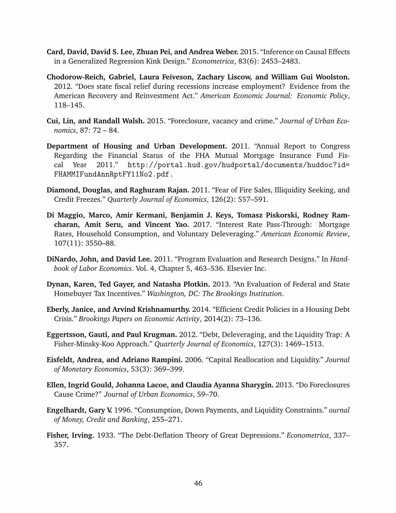
Card, David, David S. Lee, Zhuan Pei, and Andrea Weber. 2015. “Inference on Causal Effectsin a Generalized Regression Kink Design.” Econometrica, 83(6): 2453–2483.

Chodorow-Reich, Gabriel, Laura Feiveson, Zachary Liscow, and William Gui Woolston.2012. “Does state fiscal relief during recessions increase employment? Evidence from theAmerican Recovery and Reinvestment Act.” American Economic Journal: Economic Policy,118–145.

Cui, Lin, and Randall Walsh. 2015. “Foreclosure, vacancy and crime.” Journal of Urban Eco-nomics, 87: 72 – 84.

Department of Housing and Urban Development. 2011. “Annual Report to CongressRegarding the Financial Status of the FHA Mutual Mortgage Insurance Fund Fis-cal Year 2011.” http://portal.hud.gov/hudportal/documents/huddoc?id=FHAMMIFundAnnRptFY11No2.pdf.

Diamond, Douglas, and Raghuram Rajan. 2011. “Fear of Fire Sales, Illiquidity Seeking, andCredit Freezes.” Quarterly Journal of Economics, 126(2): 557–591.

Di Maggio, Marco, Amir Kermani, Benjamin J. Keys, Tomasz Piskorski, Rodney Ram-charan, Amit Seru, and Vincent Yao. 2017. “Interest Rate Pass-Through: MortgageRates, Household Consumption, and Voluntary Deleveraging.” American Economic Review,107(11): 3550–88.

DiNardo, John, and David Lee. 2011. “Program Evaluation and Research Designs.” In Hand-book of Labor Economics. Vol. 4, Chapter 5, 463–536. Elsevier Inc.

Dynan, Karen, Ted Gayer, and Natasha Plotkin. 2013. “An Evaluation of Federal and StateHomebuyer Tax Incentives.” Washington, DC: The Brookings Institution.

Eberly, Janice, and Arvind Krishnamurthy. 2014. “Efficient Credit Policies in a Housing DebtCrisis.” Brookings Papers on Economic Activity, 2014(2): 73–136.

Eggertsson, Gauti, and Paul Krugman. 2012. “Debt, Deleveraging, and the Liquidity Trap: AFisher-Minsky-Koo Approach.” Quarterly Journal of Economics, 127(3): 1469–1513.

Eisfeldt, Andrea, and Adriano Rampini. 2006. “Capital Reallocation and Liquidity.” Journalof Monetary Economics, 53(3): 369–399.

Ellen, Ingrid Gould, Johanna Lacoe, and Claudia Ayanna Sharygin. 2013. “Do ForeclosuresCause Crime?” Journal of Urban Economics, 59–70.

Engelhardt, Gary V. 1996. “Consumption, Down Payments, and Liquidity Constraints.” ournalof Money, Credit and Banking, 255–271.

Fisher, Irving. 1933. “The Debt-Deflation Theory of Great Depressions.” Econometrica, 337–357.

46

French, Kenneth, Martin Baily, John Campbell, John Cochrane, Douglas Diamond, DarrellDuffie, Anil Kashyap, Frederic Mishkin, Raghuram Rajan, David Scharfstein, et al. 2010.The Squam Lake Report: Fixing the Financial System. Princeton University Press.

Gerardi, Kristopher, Eric Rosenblatt, Paul S. Willen, and Vincent Yao. 2015. “Foreclosureexternalities: New evidence.” Journal of Urban Economics, 87: 42 – 56.

Glaeser, Edward L., and Jesse M. Shapiro. 2003. “The Benefits of the Home Mortgage InterestDeduction.” Tax Policy and the Economy, 17: 37–82.

Goodman, Laurie, Ellen Seidman, and Jun Zhu. 2014. “FHA Loan Limits: What Areas Arethe Most Affected?” Urban Institute.

Green, Daniel, Brian T. Melzer, Jonathan A. Parker, and Arcenis Rojas. 2016. “Acceleratoror Brake? Cash for Clunkers, Household Liquidity, and Aggregate Demand.” NBER WorkingPaper No. 22878.

Guren, Adam M., and Timothy J. McQuade. 2015. “How Do Foreclosures Exacerbate HousingDownturns?” Working Paper.

Hanson, Samuel, Anil Kashyap, and Jeremy Stein. 2011. “A Macroprudential Approach toFinancial Regulation.” Journal of Economic Perspectives, 25(1): 3–28.

Hayek, Friedrich von. 1931. “The "Paradox" of Saving.” Economica, 32: 125–169.

Hedlund, Aaron. 2016. “Illiquidity and its discontents: Trading delays and foreclosures in thehousing market.” Journal of Monetary Economics, 83(7): 1–13.

Hembre, Erik. 2015. “The Price of Homeowners: An Examination of the First-time HomebuyerTax Credit.” Working Paper.

House, Christopher, and Matthew Shapiro. 2008. “Temporary Investment Tax Incentives:Theory with Evidence from Bonus Depreciation.” American Economic Review, 98(3): 737–68.

Iacoviello, Matteo. 2005. “House Prices, Borrowing Constraints and Monetary Policy in theBusiness Cycle.” American Economic Review, 739–764.

Kaplan, Greg, Kurt Mitman, and Gianluca Violante. 2016. “Non-durable Consumption andHousing Net Worth in the Great Recession: Evidence from Easily Accessible Data.” NBERWorking Papers 22232.

Keynes, John Maynard. 1936. The General Theory of Employment, Interest, and Money. London:Macmillan.

Kirker, Michael, Max Floetotto, and Johannes Stroebel. 2016. “Government Intervention inthe Housing Market: Who Wins, Who Loses?” Journal of Monetary Economics, 80: 106–123.

Kiyotaki, Nobuhiro, and John Moore. 1997. “Credit Cycles.” Journal of Political Economy,105(21): 211–248.

47

Kolko, Jed. 2012. “Consumer Optimism: Too Much of a Good Thing?” http://www.trulia.com/blog/trends/trulia-american-dream-survey/, Accessed: 2016-06-15.

Lorenzoni, Guido. 2008. “Inefficient Credit Booms.” Review of Economic Studies, 75(3): 809–833.

Manoli, Dayanand, and Nicholas Turner. 2018. “Cash-on-Hand and College Enrollment: Ev-idence from Population Tax Data and Policy Nonlinearities.” Working Paper.

Mian, Atif, Amir Sufi, and Francesco Trebbi. 2015. “Foreclosures, House Prices, and the RealEconomy.” Journal of Finance, 2587–2634.

Mian, Atif, and Amir Sufi. 2009. “The consequences of mortgage credit expansion: Evidencefrom the US mortgage default crisis.” Quarterly Journal of Economics, 124(4): 1449.

Mian, Atif, and Amir Sufi. 2011. “House Prices, Home Equity-Based Borrowing, and the U.S.Household Leverage Crisis.” American Economic Review, 2132–2156.

Mian, Atif, and Amir Sufi. 2012. “The Effects of Fiscal Stimulus: Evidence from the 2009 Cashfor Clunkers Program.” Quarterly Journal of Economics, 1107–1142.

Mian, Atif, and Amir Sufi. 2014. “What Explains the 2007-2009 Drop in Employment?” Econo-metrica, 2197–2223.

Mian, Atif, and Amir Sufi. 2015. House of Debt: How They (and You) Caused the Great Recession,and How We Can Prevent It from Happening Again. University of Chicago Press.

Mian, Atif, Kamelesh Rao, and Amir Sufi. 2013. “Household Balance Sheets, Consumption,and the Economic Slump.” Quarterly Journal of Economics, 1687–1726.

National Association of Realtors. 2010. “Profile of Home Buyers and Sellers 2010.”

Nielsen, Helena Skyt, Torben Sørensen, and Christopher Taber. 2010. “Estimating the Effectof Student Aid on College Enrollment: Evidence from a Government Grant Policy Reform.”American Economic Journal: Economic Policy, 2(2): 185–215.

Ramey, Valerie, and Matthew Shapiro. 2001. “Displaced Capital: A Study of Aerospace PlantClosings.” Journal of Political Economy, 109(5): 958–992.

Rognlie, Matthew, Andrei Shleifer, and Alp Simsek. 2014. “Investment Hangover and theGreat Recession.” NBER Working Paper No. 20569.

Shleifer, Andrei, and Robert Vishny. 1992. “Liquidation Values and Debt Capacity: A MarketEquilibrium Approach.” Journal of Finance, 47(4): 1343–1366.

Shleifer, Andrei, and Robert Vishny. 2010a. “Asset Fire Sales and Credit Easing.” AmericanEconomic Review: Papers and Proceedings, 100(2): 46–50.

Shleifer, Andrei, and Robert Vishny. 2010b. “Unstable Banking.” Journal of Financial Eco-nomics, 97(3): 306–318.

48

Stein, Jeremy. 1995. “Prices and Trading Volume in the Housing Market: A Model with Down-Payment Effects.” Quarterly Journal of Economics, 379–406.

Stroebel, Johannes, and Joseph Vavra. 2016. “House Prices, Local Demand, and RetailPrices.” NBER Working Papers 20710.

Whitaker, Stephen, and Thomas J Fitzpatrick IV. 2013. “Deconstructing Distressed-PropertySpillovers: The Effects of Vacant, Tax-Delinquent, and Foreclosed Properties in Housing Sub-markets.” Journal of Housing Economics, 22(2): 79–91.

Zwick, Eric, and James Mahon. 2017. “Tax Policy and Heterogeneous Investment Behavior.”American Economic Review, 107(1): 217–48.

49

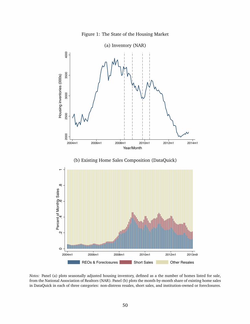
Figure 1: The State of the Housing Market

(a) Inventory (NAR)

2000

2500

3000

3500

4000

Hou

sing

inve

ntor

ies

(000

s)

2004m1 2006m1 2008m1 2010m1 2012m1 2014m1Year/Month

(b) Existing Home Sales Composition (DataQuick)

0.2

.4.6

.81

Perc

ent o

f Mon

thly

Sale

s

2004m1 2006m1 2008m1 2010m1 2012m1 2013m9

REOs & Foreclosures Short Sales Other Resales

Notes: Panel (a) plots seasonally adjusted housing inventory, defined as a the number of homes listed for sale,from the National Association of Realtors (NAR). Panel (b) plots the month-by-month share of existing home salesin DataQuick in each of three categories: non-distress resales, short sales, and institution-owned or foreclosures.

50

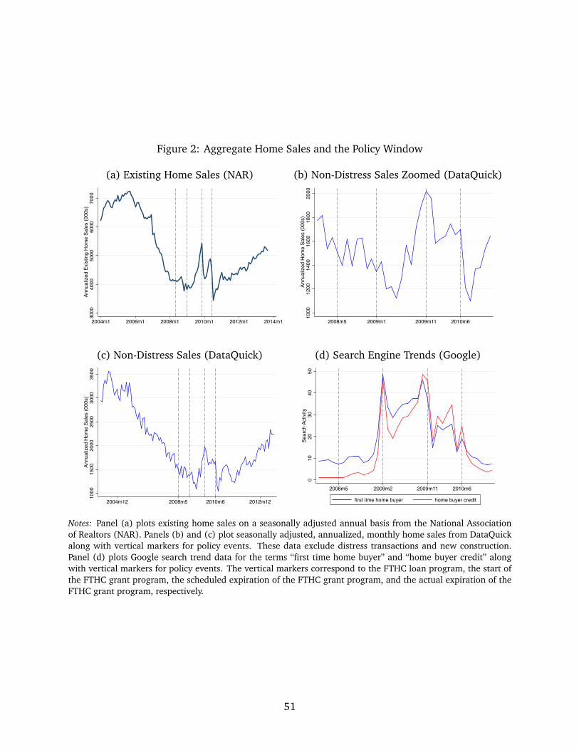
Figure 2: Aggregate Home Sales and the Policy Window

(a) Existing Home Sales (NAR) (b) Non-Distress Sales Zoomed (DataQuick)

3000

4000

5000

6000

7000

Annu

aliz

ed E

xist

ing

Hom

e Sa

les

(000

s)

2004m1 2006m1 2008m1 2010m1 2012m1 2014m1

1000

1200

1400

1600

1800

2000

Annu

aliz

ed H

ome

Sale

s (0

00s)

2008m5 2009m1 2009m11 2010m6

(c) Non-Distress Sales (DataQuick) (d) Search Engine Trends (Google)

1000

1500

2000

2500

3000

3500

Annu

aliz

ed H

ome

Sale

s (0

00s)

2004m12 2008m5 2010m6 2012m12

010

2030

4050

Sear

ch A

ctiv

ity

2008m5 2009m2 2009m11 2010m6

first time home buyer home buyer credit

Notes: Panel (a) plots existing home sales on a seasonally adjusted annual basis from the National Associationof Realtors (NAR). Panels (b) and (c) plot seasonally adjusted, annualized, monthly home sales from DataQuickalong with vertical markers for policy events. These data exclude distress transactions and new construction.Panel (d) plots Google search trend data for the terms “first time home buyer” and “home buyer credit” alongwith vertical markers for policy events. The vertical markers correspond to the FTHC loan program, the start ofthe FTHC grant program, the scheduled expiration of the FTHC grant program, and the actual expiration of theFTHC grant program, respectively.

51

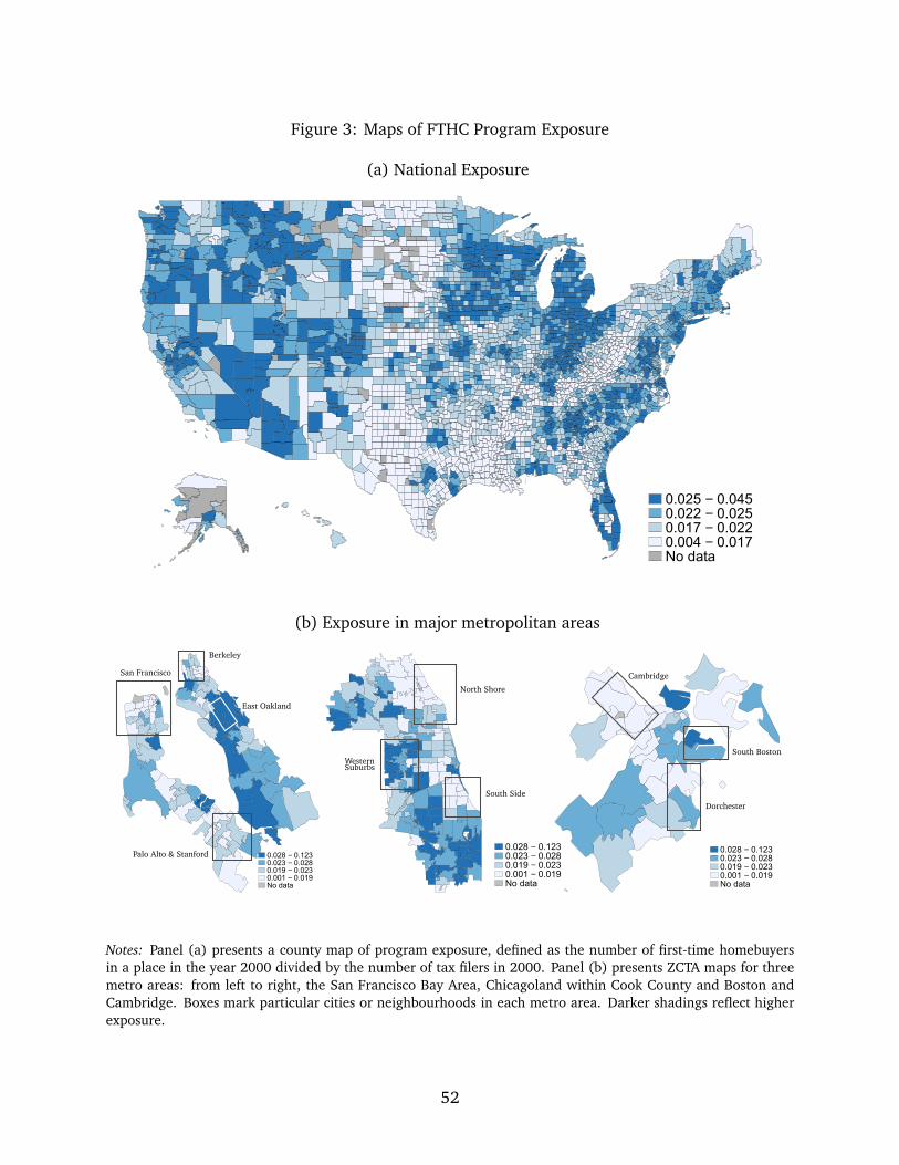
Figure 3: Maps of FTHC Program Exposure

(a) National Exposure

0.025 − 0.0450.022 − 0.0250.017 − 0.0220.004 − 0.017No data

(b) Exposure in major metropolitan areas

0.028 − 0.1230.023 − 0.0280.019 − 0.0230.001 − 0.019No data

San Francisco

Berkeley

East Oakland

Palo Alto & Stanford0.028 − 0.1230.023 − 0.0280.019 − 0.0230.001 − 0.019No data

South Side

North Shore

WesternSuburbs

0.028 − 0.1230.023 − 0.0280.019 − 0.0230.001 − 0.019No data

Cambridge

South Boston

Dorchester

Notes: Panel (a) presents a county map of program exposure, defined as the number of first-time homebuyersin a place in the year 2000 divided by the number of tax filers in 2000. Panel (b) presents ZCTA maps for threemetro areas: from left to right, the San Francisco Bay Area, Chicagoland within Cook County and Boston andCambridge. Boxes mark particular cities or neighbourhoods in each metro area. Darker shadings reflect higherexposure.

52

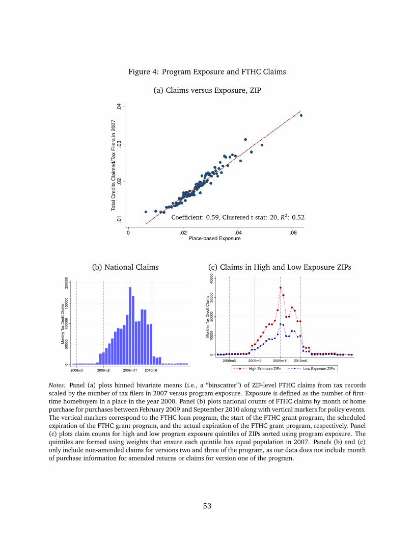
Figure 4: Program Exposure and FTHC Claims

(a) Claims versus Exposure, ZIP

.01

.02

.03

.04

Tota

l Cre

dits

Cla

imed

/Tax

File

rs in

200

7

0 .02 .04 .06Place-based Exposure

Coefficient: 0.59, Clustered t-stat: 20, R2: 0.52

(b) National Claims (c) Claims in High and Low Exposure ZIPs

050

000

1000

0015

0000

2000

00M

onth

ly T

ax C

redi

t Cla

ims

2008m5 2009m2 2009m11 2010m6

010

000

2000

030

000

4000

0M

onth

ly T

ax C

redi

t Cla

ims

2008m5 2009m2 2009m11 2010m6

High Exposure ZIPs Low Exposure ZIPs

Notes: Panel (a) plots binned bivariate means (i.e., a “binscatter”) of ZIP-level FTHC claims from tax recordsscaled by the number of tax filers in 2007 versus program exposure. Exposure is defined as the number of first-time homebuyers in a place in the year 2000. Panel (b) plots national counts of FTHC claims by month of homepurchase for purchases between February 2009 and September 2010 along with vertical markers for policy events.The vertical markers correspond to the FTHC loan program, the start of the FTHC grant program, the scheduledexpiration of the FTHC grant program, and the actual expiration of the FTHC grant program, respectively. Panel(c) plots claim counts for high and low program exposure quintiles of ZIPs sorted using program exposure. Thequintiles are formed using weights that ensure each quintile has equal population in 2007. Panels (b) and (c)only include non-amended claims for versions two and three of the program, as our data does not include monthof purchase information for amended returns or claims for version one of the program.

53

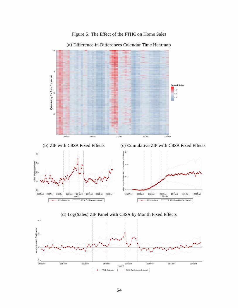
Figure 5: The Effect of the FTHC on Home Sales

(a) Difference-in-Differences Calendar Time Heatmap

25

50

75

100

2008m1 2009m1 2010m1 2011m1 2011m11

Qua

ntile

by

Ex

Ant

e E

xpos

ure

0.6

0.8

1.0

Scaled Sales

(b) ZIP with CBSA Fixed Effects (c) Cumulative ZIP with CBSA Fixed Effects

-.02

0.0

2.0

4.0

6Sa

les

impa

ct c

oeffi

cien

t

2006m1 2007m1 2008m1 2009m1 2010m1 2011m1 2012m1 2013m1Month

With Controls 95% Confidence Interval

0.5

11.

5Sa

les

impa

ct c

oeffi

cien

t, cu

mul

ativ

e pu

rcha

ses

2007m1 2008m1 2009m1 2010m1 2011m1 2012m1 2013m1Month

With controls 95% Confidence Interval

(d) Log(Sales) ZIP Panel with CBSA-by-Month Fixed Effects

-.05

0.0

5.1

Mon

th-b

y-M

onth

Coe

ffici

ents

2006m1 2007m1 2008m1 2009m1 2010m1 2011m1 2012m1 2013m1Month

With Controls 95% Confidence Interval

54

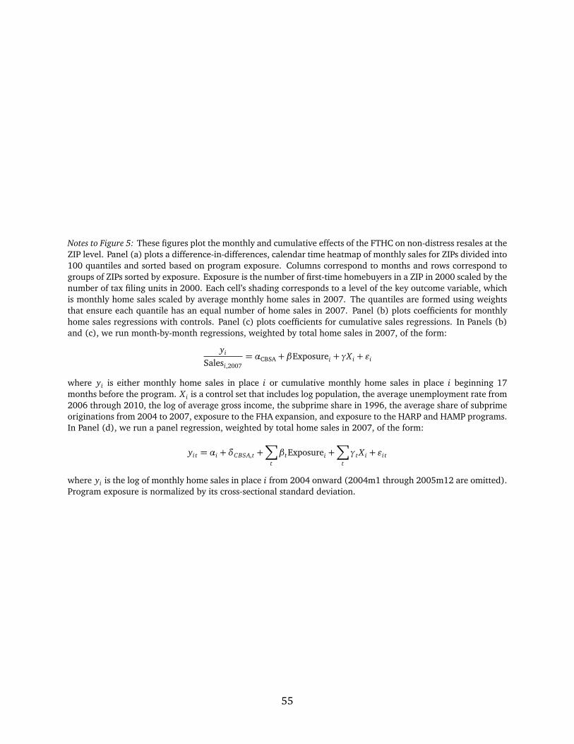
Notes to Figure 5: These figures plot the monthly and cumulative effects of the FTHC on non-distress resales at theZIP level. Panel (a) plots a difference-in-differences, calendar time heatmap of monthly sales for ZIPs divided into100 quantiles and sorted based on program exposure. Columns correspond to months and rows correspond togroups of ZIPs sorted by exposure. Exposure is the number of first-time homebuyers in a ZIP in 2000 scaled by thenumber of tax filing units in 2000. Each cell’s shading corresponds to a level of the key outcome variable, whichis monthly home sales scaled by average monthly home sales in 2007. The quantiles are formed using weightsthat ensure each quantile has an equal number of home sales in 2007. Panel (b) plots coefficients for monthlyhome sales regressions with controls. Panel (c) plots coefficients for cumulative sales regressions. In Panels (b)and (c), we run month-by-month regressions, weighted by total home sales in 2007, of the form:

yi

Salesi,2007= αCBSA + βExposurei + γX i + εi

where yi is either monthly home sales in place i or cumulative monthly home sales in place i beginning 17months before the program. X i is a control set that includes log population, the average unemployment rate from2006 through 2010, the log of average gross income, the subprime share in 1996, the average share of subprimeoriginations from 2004 to 2007, exposure to the FHA expansion, and exposure to the HARP and HAMP programs.In Panel (d), we run a panel regression, weighted by total home sales in 2007, of the form:

yi t = αi +δCBSA,t +∑

t

βtExposurei +∑

t

γt X i + εi t

where yi is the log of monthly home sales in place i from 2004 onward (2004m1 through 2005m12 are omitted).Program exposure is normalized by its cross-sectional standard deviation.

55

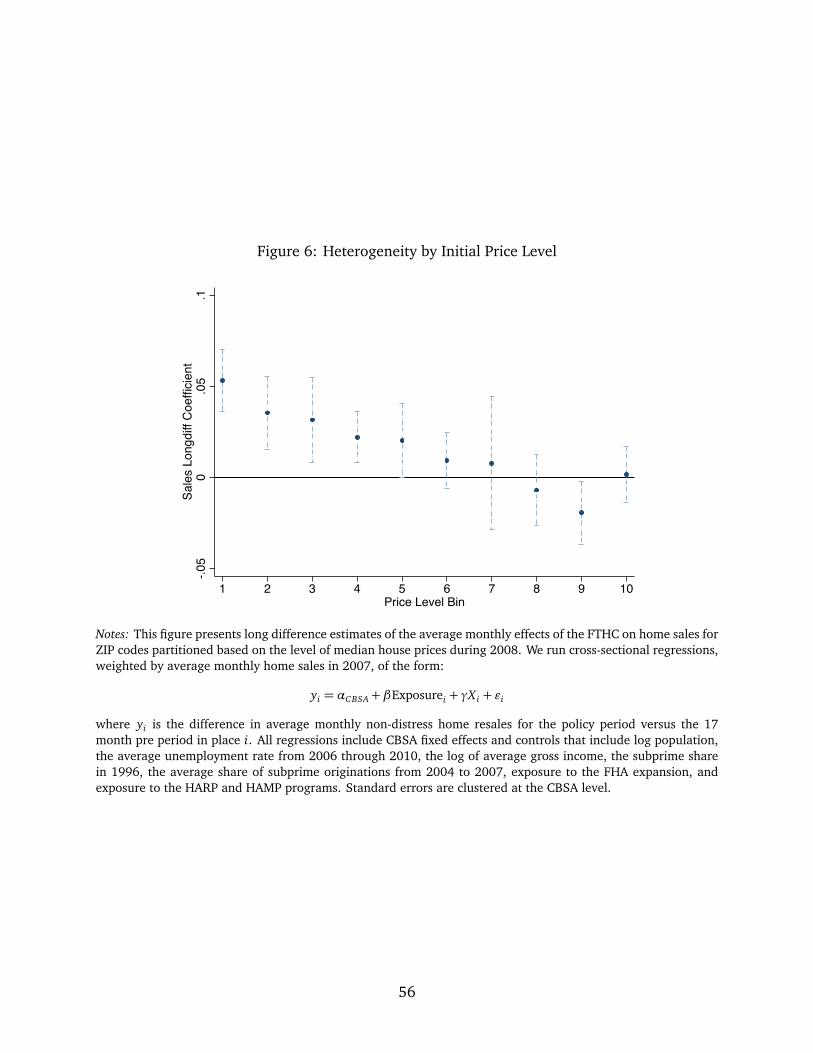
Figure 6: Heterogeneity by Initial Price Level

-.05

0.0

5.1

Sale

s Lo

ngdi

ff C

oeffi

cien

t

1 2 3 4 5 6 7 8 9 10Price Level Bin

Notes: This figure presents long difference estimates of the average monthly effects of the FTHC on home sales forZIP codes partitioned based on the level of median house prices during 2008. We run cross-sectional regressions,weighted by average monthly home sales in 2007, of the form:

yi = αCBSA+ βExposurei + γX i + εi

where yi is the difference in average monthly non-distress home resales for the policy period versus the 17month pre period in place i. All regressions include CBSA fixed effects and controls that include log population,the average unemployment rate from 2006 through 2010, the log of average gross income, the subprime sharein 1996, the average share of subprime originations from 2004 to 2007, exposure to the FHA expansion, andexposure to the HARP and HAMP programs. Standard errors are clustered at the CBSA level.

56

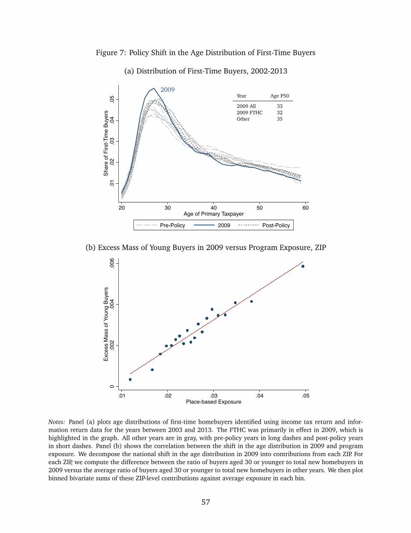
Figure 7: Policy Shift in the Age Distribution of First-Time Buyers

(a) Distribution of First-Time Buyers, 2002-2013

.01

.02

.03

.04

.05

Shar

e of

Firs

t-Tim

e Bu

yers

20 30 40 50 60Age of Primary Taxpayer

Pre-Policy 2009 Post-Policy

2009Year Age P50

2009 All 332009 FTHC 32Other 35

(b) Excess Mass of Young Buyers in 2009 versus Program Exposure, ZIP

0.0

02.0

04.0

06Ex

cess

Mas

s of

You

ng B

uyer

s

.01 .02 .03 .04 .05Place-based Exposure

Notes: Panel (a) plots age distributions of first-time homebuyers identified using income tax return and infor-mation return data for the years between 2003 and 2013. The FTHC was primarily in effect in 2009, which ishighlighted in the graph. All other years are in gray, with pre-policy years in long dashes and post-policy yearsin short dashes. Panel (b) shows the correlation between the shift in the age distribution in 2009 and programexposure. We decompose the national shift in the age distribution in 2009 into contributions from each ZIP. Foreach ZIP, we compute the difference between the ratio of buyers aged 30 or younger to total new homebuyers in2009 versus the average ratio of buyers aged 30 or younger to total new homebuyers in other years. We then plotbinned bivariate sums of these ZIP-level contributions against average exposure in each bin.

57

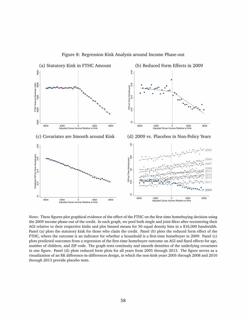
Figure 8: Regression Kink Analysis around Income Phase-out

(a) Statutory Kink in FTHC Amount (b) Reduced Form Effects in 2009

5000

6000

7000

8000

9000

FTH

C A

mou

nt (N

omin

al U

SD)

-8000 -4000 0 4000 8000Adjusted Gross Income Relative to Kink

.01

.012

.014

.016

.018

P(Fi

rst-T

ime

Hom

ebuy

er)

-8000 -4000 0 4000 8000Adjusted Gross Income Relative to Kink

(c) Covariates are Smooth around Kink (d) 2009 vs. Placebos in Non-Policy Years

.01

.012

.014

.016

.018

Pred

icte

d P(

Firs

t-Tim

e H

omeb

uyer

)

-8000 -4000 0 4000 8000Adjusted Gross Income Relative to Kink

.01

.015

.02

.025

.03

P(Fi

rst-T

ime

Hom

ebuy

er)

-8000 -4000 0 4000 8000Adjusted Gross Income Relative to Kink

2009

2005

2006200720082013201020122011

Notes: These figures plot graphical evidence of the effect of the FTHC on the first-time homebuying decision usingthe 2009 income phase-out of the credit. In each graph, we pool both single and joint filers after recentering theirAGI relative to their respective kinks and plot binned means for 50 equal density bins in a $16,000 bandwidth.Panel (a) plots the statutory kink for those who claim the credit. Panel (b) plots the reduced form effect of theFTHC, where the outcome is an indicator for whether a household is a first-time homebuyer in 2009. Panel (c)plots predicted outcomes from a regression of the first-time homebuyer outcome on AGI and fixed effects for age,number of children, and ZIP code. The graph tests continuity and smooth densities of the underlying covariatesin one figure. Panel (d) plots reduced form plots for all years from 2005 through 2013. The figure serves as avisualization of an RK difference-in-differences design, in which the non-kink years 2005 through 2008 and 2010through 2013 provide placebo tests.

58

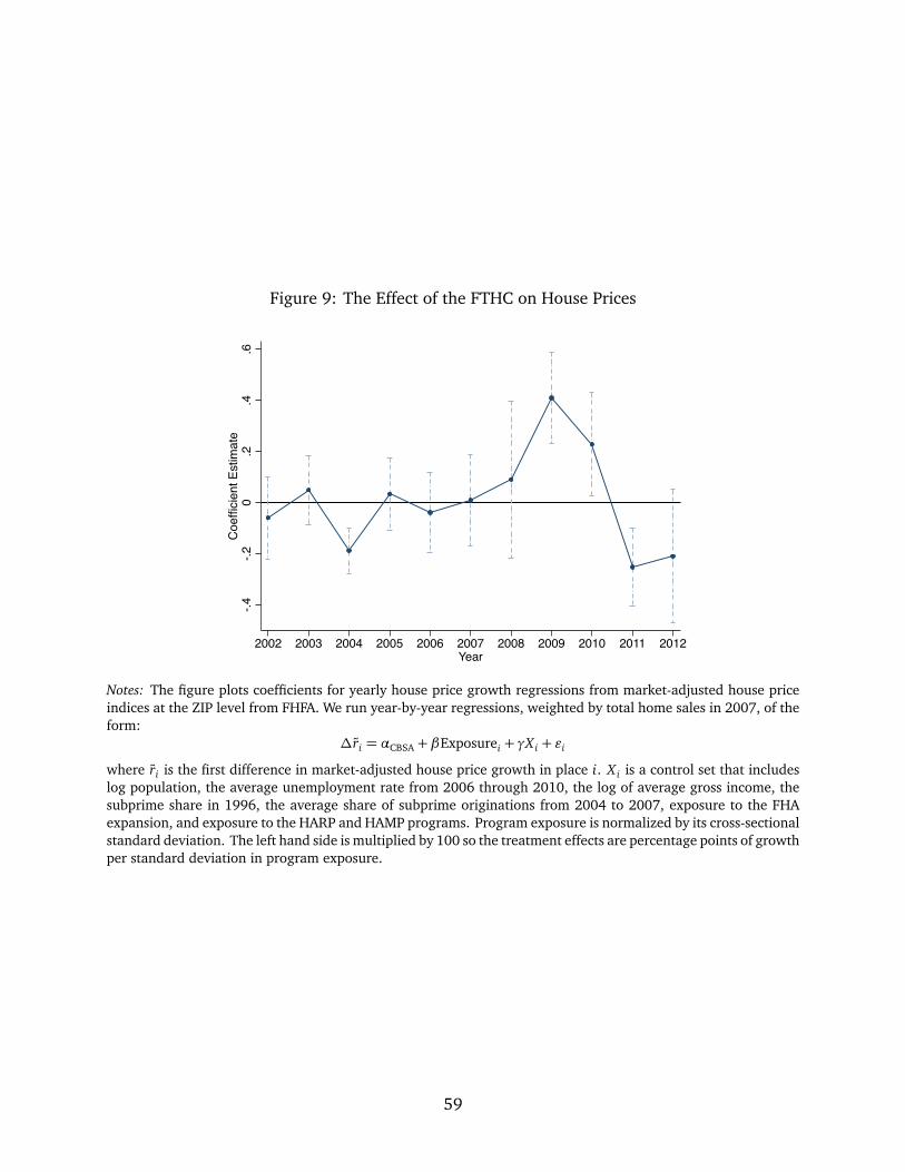
Figure 9: The Effect of the FTHC on House Prices

-.4-.2

0.2

.4.6

Coe

ffici

ent E

stim

ate

2002 2003 2004 2005 2006 2007 2008 2009 2010 2011 2012Year

Notes: The figure plots coefficients for yearly house price growth regressions from market-adjusted house priceindices at the ZIP level from FHFA. We run year-by-year regressions, weighted by total home sales in 2007, of theform:

∆r̃i = αCBSA + βExposurei + γX i + εi

where r̃i is the first difference in market-adjusted house price growth in place i. X i is a control set that includeslog population, the average unemployment rate from 2006 through 2010, the log of average gross income, thesubprime share in 1996, the average share of subprime originations from 2004 to 2007, exposure to the FHAexpansion, and exposure to the HARP and HAMP programs. Program exposure is normalized by its cross-sectionalstandard deviation. The left hand side is multiplied by 100 so the treatment effects are percentage points of growthper standard deviation in program exposure.

59

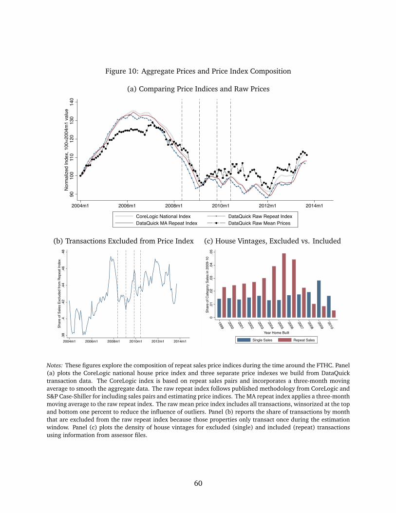
Figure 10: Aggregate Prices and Price Index Composition

(a) Comparing Price Indices and Raw Prices

9010

011

012

013

014

0N

orm

aliz

ed In

dex,

100

=200

4m1

valu

e

2004m1 2006m1 2008m1 2010m1 2012m1 2014m1

CoreLogic National Index DataQuick Raw Repeat IndexDataQuick MA Repeat Index DataQuick Raw Mean Prices

(b) Transactions Excluded from Price Index (c) House Vintages, Excluded vs. Included

.38

.4.4

2.4

4.4

6.4

8Sh

are

of S

ales

Exc

lude

d fro

m R

epea

t Ind

ex

2004m1 2006m1 2008m1 2010m1 2012m1 2014m1

0.0

1.0

2.0

3.0

4.0

5Sh

are

of C

ateg

ory

Sale

s in

200

9-10

1999

2000

2001

2002

2003

2004

2005

2006

2007

2008

2009

2010

Year Home Built

Single Sales Repeat Sales

Notes: These figures explore the composition of repeat sales price indices during the time around the FTHC. Panel(a) plots the CoreLogic national house price index and three separate price indexes we build from DataQuicktransaction data. The CoreLogic index is based on repeat sales pairs and incorporates a three-month movingaverage to smooth the aggregate data. The raw repeat index follows published methodology from CoreLogic andS&P Case-Shiller for including sales pairs and estimating price indices. The MA repeat index applies a three-monthmoving average to the raw repeat index. The raw mean price index includes all transactions, winsorized at the topand bottom one percent to reduce the influence of outliers. Panel (b) reports the share of transactions by monththat are excluded from the raw repeat index because those properties only transact once during the estimationwindow. Panel (c) plots the density of house vintages for excluded (single) and included (repeat) transactionsusing information from assessor files.

60

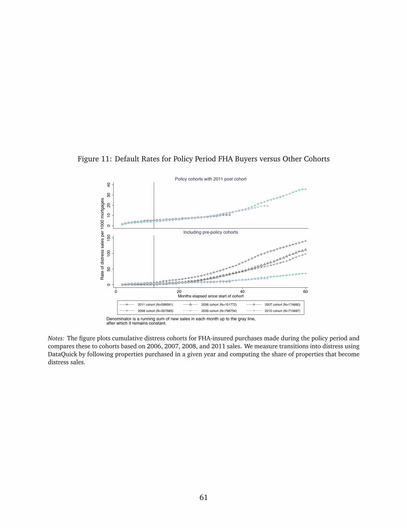
Figure 11: Default Rates for Policy Period FHA Buyers versus Other Cohorts

010

2030

40

Policy cohorts with 2011 post cohort

050

100

150

0 20 40 60Months elapsed since start of cohort

2011 cohort (N=599581) 2006 cohort (N=151772) 2007 cohort (N=174660)

2008 cohort (N=557685) 2009 cohort (N=798754) 2010 cohort (N=715687)

Including pre-policy cohorts

Denominator is a running sum of new sales in each month up to the gray line,after which it remains constant.

Rat

e of

dis

tress

sal

es p

er 1

000

mor

tgag

es

Notes: The figure plots cumulative distress cohorts for FHA-insured purchases made during the policy period andcompares these to cohorts based on 2006, 2007, 2008, and 2011 sales. We measure transitions into distress usingDataQuick by following properties purchased in a given year and computing the share of properties that becomedistress sales.

61

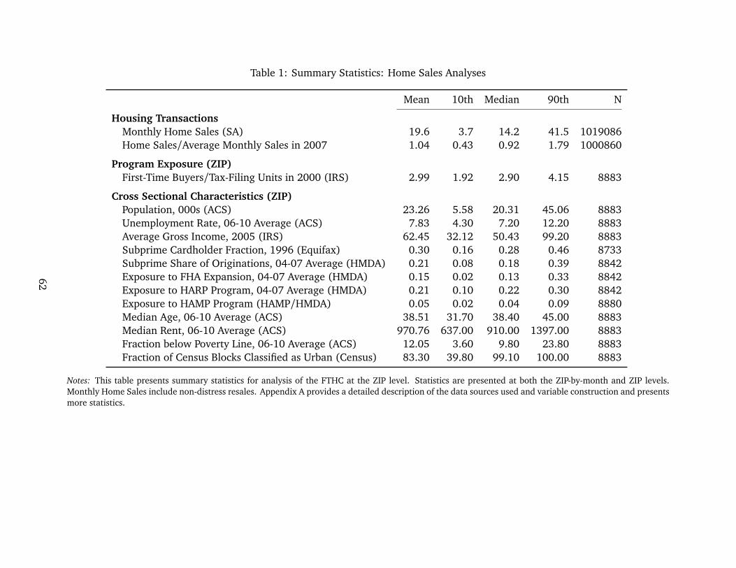
Table 1: Summary Statistics: Home Sales Analyses

Mean 10th Median 90th N

Housing TransactionsMonthly Home Sales (SA) 19.6 3.7 14.2 41.5 1019086Home Sales/Average Monthly Sales in 2007 1.04 0.43 0.92 1.79 1000860

Program Exposure (ZIP)First-Time Buyers/Tax-Filing Units in 2000 (IRS) 2.99 1.92 2.90 4.15 8883

Cross Sectional Characteristics (ZIP)Population, 000s (ACS) 23.26 5.58 20.31 45.06 8883Unemployment Rate, 06-10 Average (ACS) 7.83 4.30 7.20 12.20 8883Average Gross Income, 2005 (IRS) 62.45 32.12 50.43 99.20 8883Subprime Cardholder Fraction, 1996 (Equifax) 0.30 0.16 0.28 0.46 8733Subprime Share of Originations, 04-07 Average (HMDA) 0.21 0.08 0.18 0.39 8842Exposure to FHA Expansion, 04-07 Average (HMDA) 0.15 0.02 0.13 0.33 8842Exposure to HARP Program, 04-07 Average (HMDA) 0.21 0.10 0.22 0.30 8842Exposure to HAMP Program (HAMP/HMDA) 0.05 0.02 0.04 0.09 8880Median Age, 06-10 Average (ACS) 38.51 31.70 38.40 45.00 8883Median Rent, 06-10 Average (ACS) 970.76 637.00 910.00 1397.00 8883Fraction below Poverty Line, 06-10 Average (ACS) 12.05 3.60 9.80 23.80 8883Fraction of Census Blocks Classified as Urban (Census) 83.30 39.80 99.10 100.00 8883

Notes: This table presents summary statistics for analysis of the FTHC at the ZIP level. Statistics are presented at both the ZIP-by-month and ZIP levels.Monthly Home Sales include non-distress resales. Appendix A provides a detailed description of the data sources used and variable construction and presentsmore statistics.

62

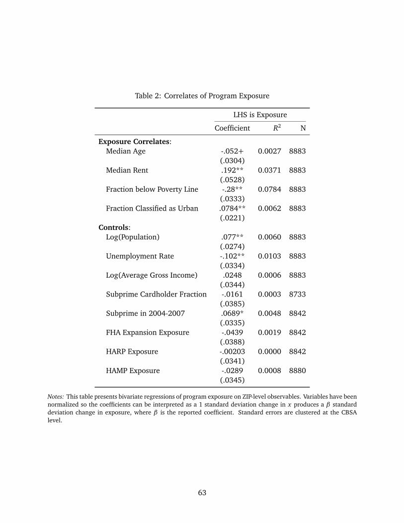
Table 2: Correlates of Program Exposure

LHS is Exposure

Coefficient R2 N

Exposure Correlates:Median Age -.052+ 0.0027 8883

(.0304)Median Rent .192** 0.0371 8883

(.0528)Fraction below Poverty Line -.28** 0.0784 8883

(.0333)Fraction Classified as Urban .0784** 0.0062 8883

(.0221)Controls:

Log(Population) .077** 0.0060 8883(.0274)

Unemployment Rate -.102** 0.0103 8883(.0334)

Log(Average Gross Income) .0248 0.0006 8883(.0344)

Subprime Cardholder Fraction -.0161 0.0003 8733(.0385)

Subprime in 2004-2007 .0689* 0.0048 8842(.0335)

FHA Expansion Exposure -.0439 0.0019 8842(.0388)

HARP Exposure -.00203 0.0000 8842(.0341)

HAMP Exposure -.0289 0.0008 8880(.0345)

Notes: This table presents bivariate regressions of program exposure on ZIP-level observables. Variables have beennormalized so the coefficients can be interpreted as a 1 standard deviation change in x produces a β standarddeviation change in exposure, where β is the reported coefficient. Standard errors are clustered at the CBSAlevel.

63

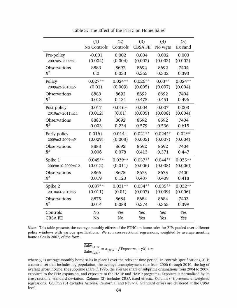
Table 3: The Effect of the FTHC on Home Sales

(1) (2) (3) (4) (5)No Controls Controls CBSA FE No wgts Ex sand

Pre-policy -0.001 0.002 0.004 0.002 0.0032007m9-2009m1 (0.004) (0.004) (0.002) (0.003) (0.002)

Observations 8883 8692 8692 8692 7404R2 0.0 0.033 0.365 0.302 0.393

Policy 0.027** 0.024** 0.026** 0.03** 0.024**2009m2-2010m6 (0.01) (0.009) (0.005) (0.007) (0.004)

Observations 8883 8692 8692 8692 7404R2 0.013 0.131 0.475 0.451 0.496

Post-policy 0.017 0.016+ 0.004 0.007 0.0032010m7-2011m11 (0.012) (0.01) (0.005) (0.008) (0.004)

Observations 8883 8692 8692 8692 7404R2 0.003 0.234 0.579 0.536 0.615

Early policy 0.016+ 0.014+ 0.021** 0.024** 0.02**2009m2-2009m9 (0.009) (0.008) (0.005) (0.007) (0.004)

Observations 8883 8692 8692 8692 7404R2 0.006 0.078 0.413 0.371 0.447

Spike 1 0.045** 0.039** 0.037** 0.044** 0.035**2009m10-2009m12 (0.012) (0.011) (0.006) (0.008) (0.006)

Observations 8866 8675 8675 8675 7400R2 0.019 0.123 0.437 0.409 0.418

Spike 2 0.037** 0.031** 0.034** 0.035** 0.032**2010m4-2010m6 (0.011) (0.01) (0.007) (0.009) (0.006)

Observations 8875 8684 8684 8684 7403R2 0.014 0.088 0.374 0.365 0.399

Controls No Yes Yes Yes YesCBSA FE No No Yes Yes Yes

Notes: This table presents the average monthly effects of the FTHC on home sales for ZIPs pooled over differentpolicy windows with various specifications. We run cross-sectional regressions, weighted by average monthlyhome sales in 2007, of the form:

Salesi,t→T

Salesi,2007= αCBSA + βExposurei + γX i + εi

where yi is average monthly home sales in place i over the relevant time period. In controls specifications, X i isa control set that includes log population, the average unemployment rate from 2006 through 2010, the log ofaverage gross income, the subprime share in 1996, the average share of subprime originations from 2004 to 2007,exposure to the FHA expansion, and exposure to the HARP and HAMP programs. Exposure is normalized by itscross-sectional standard deviation. Column (3) includes CBSA fixed effects. Column (4) presents unweightedregressions. Column (5) excludes Arizona, California, and Nevada. Standard errors are clustered at the CBSAlevel. 64

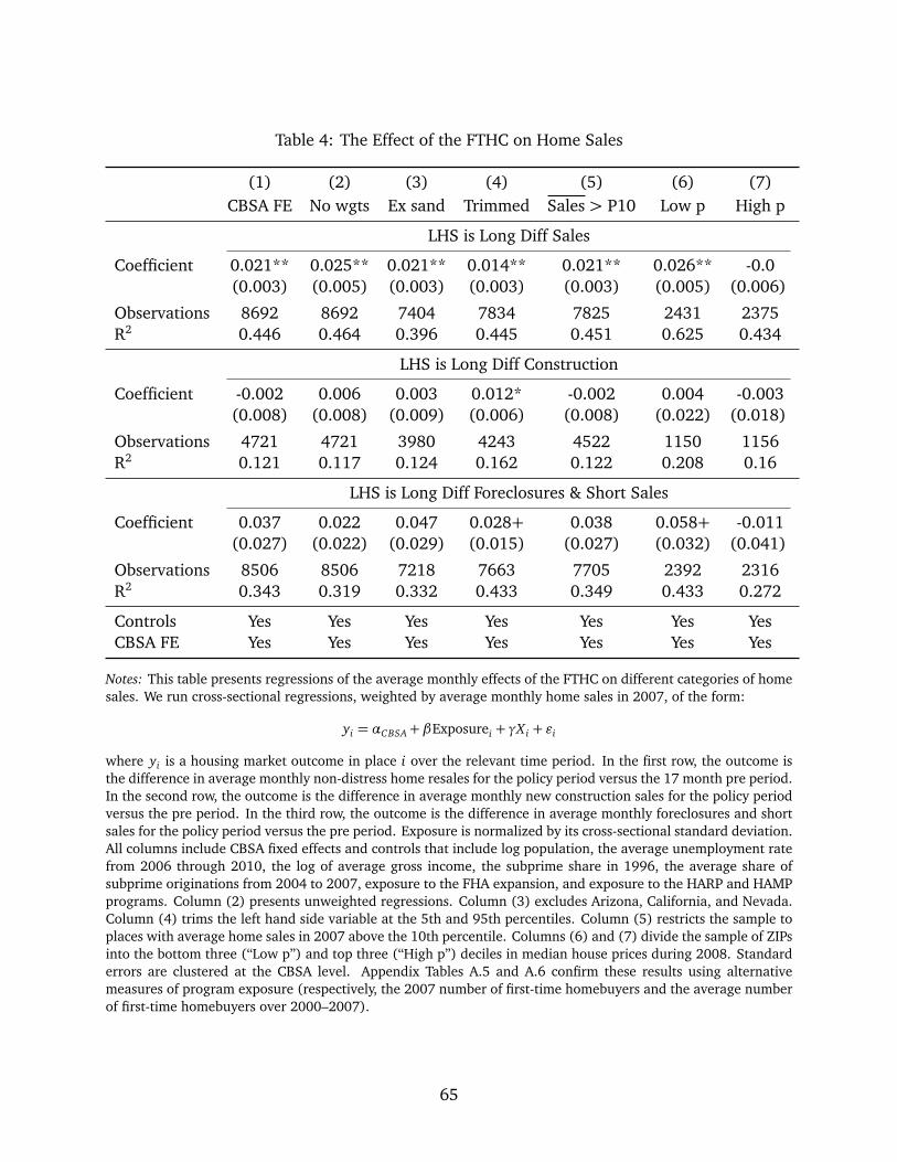
Table 4: The Effect of the FTHC on Home Sales

(1) (2) (3) (4) (5) (6) (7)CBSA FE No wgts Ex sand Trimmed Sales > P10 Low p High p

LHS is Long Diff Sales

Coefficient 0.021** 0.025** 0.021** 0.014** 0.021** 0.026** -0.0(0.003) (0.005) (0.003) (0.003) (0.003) (0.005) (0.006)

Observations 8692 8692 7404 7834 7825 2431 2375R2 0.446 0.464 0.396 0.445 0.451 0.625 0.434

LHS is Long Diff Construction

Coefficient -0.002 0.006 0.003 0.012* -0.002 0.004 -0.003(0.008) (0.008) (0.009) (0.006) (0.008) (0.022) (0.018)

Observations 4721 4721 3980 4243 4522 1150 1156R2 0.121 0.117 0.124 0.162 0.122 0.208 0.16

LHS is Long Diff Foreclosures & Short Sales

Coefficient 0.037 0.022 0.047 0.028+ 0.038 0.058+ -0.011(0.027) (0.022) (0.029) (0.015) (0.027) (0.032) (0.041)

Observations 8506 8506 7218 7663 7705 2392 2316R2 0.343 0.319 0.332 0.433 0.349 0.433 0.272

Controls Yes Yes Yes Yes Yes Yes YesCBSA FE Yes Yes Yes Yes Yes Yes Yes

Notes: This table presents regressions of the average monthly effects of the FTHC on different categories of homesales. We run cross-sectional regressions, weighted by average monthly home sales in 2007, of the form:

yi = αCBSA+ βExposurei + γX i + εi

where yi is a housing market outcome in place i over the relevant time period. In the first row, the outcome isthe difference in average monthly non-distress home resales for the policy period versus the 17 month pre period.In the second row, the outcome is the difference in average monthly new construction sales for the policy periodversus the pre period. In the third row, the outcome is the difference in average monthly foreclosures and shortsales for the policy period versus the pre period. Exposure is normalized by its cross-sectional standard deviation.All columns include CBSA fixed effects and controls that include log population, the average unemployment ratefrom 2006 through 2010, the log of average gross income, the subprime share in 1996, the average share ofsubprime originations from 2004 to 2007, exposure to the FHA expansion, and exposure to the HARP and HAMPprograms. Column (2) presents unweighted regressions. Column (3) excludes Arizona, California, and Nevada.Column (4) trims the left hand side variable at the 5th and 95th percentiles. Column (5) restricts the sample toplaces with average home sales in 2007 above the 10th percentile. Columns (6) and (7) divide the sample of ZIPsinto the bottom three (“Low p”) and top three (“High p”) deciles in median house prices during 2008. Standarderrors are clustered at the CBSA level. Appendix Tables A.5 and A.6 confirm these results using alternativemeasures of program exposure (respectively, the 2007 number of first-time homebuyers and the average numberof first-time homebuyers over 2000–2007).

65

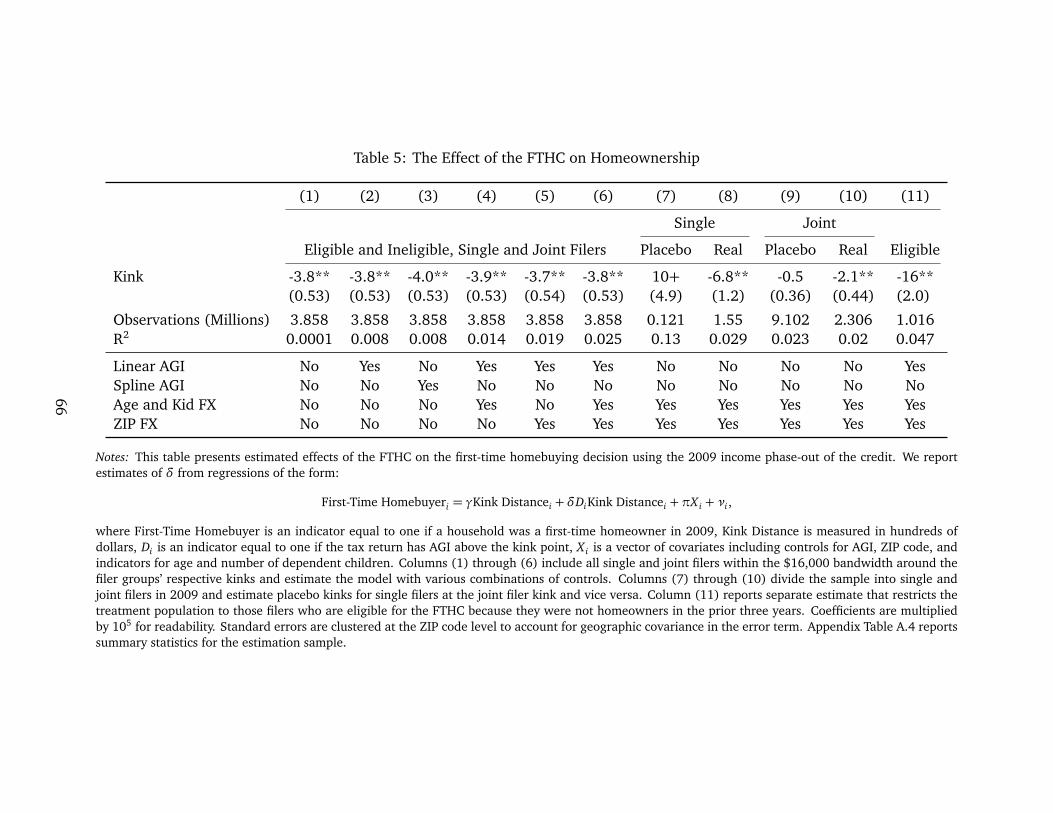
Table 5: The Effect of the FTHC on Homeownership

(1) (2) (3) (4) (5) (6) (7) (8) (9) (10) (11)

Single Joint

Eligible and Ineligible, Single and Joint Filers Placebo Real Placebo Real Eligible

Kink -3.8** -3.8** -4.0** -3.9** -3.7** -3.8** 10+ -6.8** -0.5 -2.1** -16**(0.53) (0.53) (0.53) (0.53) (0.54) (0.53) (4.9) (1.2) (0.36) (0.44) (2.0)

Observations (Millions) 3.858 3.858 3.858 3.858 3.858 3.858 0.121 1.55 9.102 2.306 1.016R2 0.0001 0.008 0.008 0.014 0.019 0.025 0.13 0.029 0.023 0.02 0.047

Linear AGI No Yes No Yes Yes Yes No No No No YesSpline AGI No No Yes No No No No No No No NoAge and Kid FX No No No Yes No Yes Yes Yes Yes Yes YesZIP FX No No No No Yes Yes Yes Yes Yes Yes Yes

Notes: This table presents estimated effects of the FTHC on the first-time homebuying decision using the 2009 income phase-out of the credit. We reportestimates of δ from regressions of the form:

First-Time Homebuyeri = γKink Distancei +δDiKink Distancei +πX i + νi ,

where First-Time Homebuyer is an indicator equal to one if a household was a first-time homeowner in 2009, Kink Distance is measured in hundreds ofdollars, Di is an indicator equal to one if the tax return has AGI above the kink point, X i is a vector of covariates including controls for AGI, ZIP code, andindicators for age and number of dependent children. Columns (1) through (6) include all single and joint filers within the $16,000 bandwidth around thefiler groups’ respective kinks and estimate the model with various combinations of controls. Columns (7) through (10) divide the sample into single andjoint filers in 2009 and estimate placebo kinks for single filers at the joint filer kink and vice versa. Column (11) reports separate estimate that restricts thetreatment population to those filers who are eligible for the FTHC because they were not homeowners in the prior three years. Coefficients are multipliedby 105 for readability. Standard errors are clustered at the ZIP code level to account for geographic covariance in the error term. Appendix Table A.4 reportssummary statistics for the estimation sample.

66

Table 6: The Effect of the FTHC on House Prices

(1) (2) (3) (4) (5) (6) (7)CBSA FE No wgts Ex sand Trimmed Sales > P10 Low p High p

LHS is Long Diff Price Growth (FHFA Mkt Adjusted)

Coefficient 1.077** 1.149** 0.946** 0.685** 1.087** 1.073** 0.628*(0.183) (0.222) (0.197) (0.125) (0.184) (0.297) (0.278)

Observations 8363 8363 7101 7523 7570 2304 2261R2 0.615 0.58 0.609 0.623 0.62 0.617 0.653

LHS is Long Diff Price Growth (FHFA Raw)

Coefficient 1.116** 1.19** 0.977** 0.714** 1.127** 1.107** 0.689*(0.193) (0.23) (0.208) (0.126) (0.194) (0.304) (0.289)

Observations 8363 8363 7101 7523 7570 2304 2261R2 0.619 0.585 0.61 0.619 0.623 0.61 0.669

LHS is Long Diff Price Growth (CoreLogic)

Coefficient 0.581** 0.597** 0.596** 0.409* 0.586** 1.2** 0.245(0.19) (0.194) (0.213) (0.186) (0.193) (0.296) (0.465)

Observations 5748 5748 4674 5175 5607 1336 1666R2 0.68 0.714 0.608 0.632 0.675 0.701 0.708

LHS is Long Diff Raw Price Growth (DataQuick)

Coefficient 1.595 1.785 1.184 0.117 1.549 0.575 0.775(1.061) (1.222) (1.207) (0.82) (1.085) (4.01) (1.677)

Observations 7308 7308 6086 6573 6851 2071 2198R2 0.088 0.092 0.076 0.1 0.089 0.147 0.147

Controls Yes Yes Yes Yes Yes Yes YesCBSA FE Yes Yes Yes Yes Yes Yes Yes

Notes: This table presents regressions of the cumulative effects of the FTHC on different measures of house pricegrowth. We run cross-sectional regressions, weighted by average monthly home sales in 2007, of the form:

yi = αCBSA+ βExposurei + γX i + εi

where yi is a housing market outcome in place i over the relevant time period. In the first row, the outcome is themarket-adjusted, cumulative annual log price differences from FHFA price index data during 2009 and 2010 minuscumulative annual log price differences during 2007 and 2008. In the second row, the outcome is the unadjustedversion of the price series from the first row. In the third row, the outcome is raw cumulative monthly log pricedifferences from CoreLogic during the policy period minus cumulative monthly log price differences during the17-month pre-period. In the fourth row, the outcome is cumulative monthly log price differences from DataQuickmean prices, winsorized at the 5 percent level, for the same pre and policy periods. In all cases, we multiplythe left hand side by 100 so the treatment effect units are percentage points of growth per standard deviationchange in program exposure. All series are seasonally adjusted prior to aggregation. Exposure is normalized by itscross-sectional standard deviation. Column (2) presents unweighted regressions. Column (3) excludes Arizona,California, and Nevada. Column (4) trims the left hand side variable at the 5th and 95th percentiles. Column (5)restricts the sample to places with average home sales in 2007 above the 10th percentile. Columns (6) and (7)divide the sample of ZIPs into the bottom three (“Low p”) and top three (“High p”) deciles in 2008 median houseprices. Standard errors are clustered at the CBSA level.67

For Online Publication

A Data Build and Discussion

The analysis combines a large number of proprietary and public use data sources. In thisappendix, we describe each source in detail, describe variable construction, and walk step-by-step through sample selection.

A.1 Data Sources and Sets

1. Tax records, IRS/OTA: These data are anonymized individual-level data collected by theIRS for the purposes of administering the tax collection process. They are made availablethrough collaboration with the Office of Tax Analysis in the US Treasury Department andthe IRS Division of Research, Analysis, and Statistics.

We compile the following items:

(a) ZIP-5 level cross sections of FTHC claims from Form 5405. These include claims forversions 2 and 3 of the FTHC program (i.e., the grant program) and also claims forthe Long-Time Homebuyer Credit.

(b) First-time homebuyer and tax filer counts from individual tax returns and informa-tion returns for the years 1998, 1999, and 2000 for measuring program exposure,and through 2013 for measuring the age of first-time homebuyers in non-policyyears.

(c) Tax filer counts for the year 2007 from individual tax returns.

Tax credit claims cover 18,073 ZIPs, the homebuyer counts from 2000 cover 24,923 ZIPs,and the 2007 records cover 35,647 ZIPs.

2. DataQuick deed records: We clean and merge data retrieved from DataQuick’s assessorfile, which contains information on individual properties used to assess property taxes,and DataQuick’s recorder file, which tracks ownership changes and loans secured byproperties.

We begin with records from 2004 to 2013, up to the company’s acquisition by CoreLogic.Assessor data cover 1,819 counties accounting for 91.8% of the US population. Whilenot all counties tracked by DataQuick provide recorder data, 942 counties do and thesematch to 88% of all deeds tracked in the assessor data.

Once the two files are joined, we produce our “canonical” list of transactions by applyingthe following filters:

(a) Including only resales and new construction (types R and S in SR_TRAN_TYPE)which are arm’s length47;

47To our knowledge, the arm’s length flag in DataQuick is the output of a “model” that classifies whetherresales are genuine arm’s length transactions. It automatically excludes refinances and intermediate documentsin a distress sale process. It attempts to exclude transactions made between related parties at non-market prices,for example, because of divorce or bequest.

68

(b) Removing transactions between institutional buyers, such as two developers or adeveloper with a GSE;

(c) Removing middle-man sales where a property buyer sells the property on the sameday;

(d) Keeping only the transaction with the highest transfer value if there are duplicateswith the same property, transaction date, buyer and seller, with the intent of remov-ing incomplete duplicate records.

We use the filtered, merged data to create three output datasets:

(a) DataQuick transaction counts. We aggregate the transactions in the recorder datato the (geographic unit)×(month)×(transaction type)×(distress type) level, wherethe geographic unit is a ZIP or county. For each level, we count the number oftransactions.This initial dataset is divided into six distinct datasets used during different parts ofthe analysis:

i. all sales (transaction types R and S, distress types ∈ NULL, A, I, S and O),ii. non-distress resales (transaction type R, null distress indicator)48

iii. new housing/subdivision sales (transaction type S),iv. purchases at foreclosure auctions (distress type A),v. DataQuick-inferred short sales (distress type I),

vi. REO liquidations (distress type S).

A variation of the above aggregation splits counts to the (geographic unit)×(month)×(transaction type)×(distress type)×(bedroom) level, where bedroom informationcomes from the assessor file. We mark each transaction as having missing bedroominformation, 1 to 3 bedrooms, or 4 or more bedrooms. Geographies with morethan 5% of months lacking transactions on properties with bedroom data, as well asgeographies in states with consistently poor bedroom data collection, are dropped.A second variation requires processing individual records further before aggrega-tion:

i. Transactions on recently built housing are marked by checking the SA_YR_BLTcolumn in the assessor file.

ii. Transactions on properties owned by developers or owned by government-sponsored enterprises are marked through running regular expression searcheson the SR_BUYER column in the recorder file. The regular expressions forbuilders, developers, and GSEs are:builder_re_list =

(’HOME|BUILDER| BUILD|BLDR| HM(\s|S\s)| CONST |REAL ESTATE|’,’PULTE|RYLAND|NVR|DR HORTON|CENTEX|LENNAR|MERITAGE|’,

48Distress type O transactions appear to be classified as distress by DataQuick, but shows no other sign of beinga distress sale, such as an unusually low sale price or institutional seller. We exclude them by default, but haveconfirmed the robustness of our results by including them as non-distress transactions. They make up at most 2%of the sample in policy period months.

69

’STANDARD PACIFIC’)developer_re_list =

(’LLC|CORP|COMPANY| INC$|INTL| LAND |PROPERT(Y|IES)|TRUST|’,’INVEST(OR|MENT)|LP’)

gse_re_list =(’FNMA|FHLM|HUD-HOUSING|FEDERAL (H|NATIONAL)|FANNIE|’,’SECRETARY OF (H|VET)|VETERANS AD’)

iii. Transactions on properties considered recently in distress are marked throughsearching over a property’s transaction history and checking if the property wasdistressed less than two years prior to the current transaction.

The exclusion of type L sales from the resales and the new housing datasets is dueto DataQuick classifying properties with a later delinquent mortgage as type L, evenif the sale associated with that mortgage was a non-distress sale. The label there-fore cannot be used to infer whether the original transaction was distressed, notdistressed, or otherwise unusual. However, these type L sales account for manytransactions in the pre-crisis period, up to a majority in some places in California.For these reasons, they are included when constructing the price and loans data.

(b) DataQuick price data: For every geographic unit-by-month unit, we compute thegroup’s median price based on the SR_VAL_TRANSFER column [for non-distressedproperties]. We exclude transactions for which price data are missing, about 10%of all transactions, from the computation. We code as missing any units wherefewer than five transactions are available. These price data serve to complementthe CoreLogic price indices in places when the CoreLogic data are not available.

(c) DataQuick loans data: DataQuick counts mortgages attached to the paperworkon a closed sale as loans related to that transaction, and allow up to three liensconnected to one transfer. However, these rows miss loans taken out by the buyerfrom different banks or subsequent to the purchase, which may include second liensand “piggyback loans” used to cover the cost of the down payment.We connect second liens, which are categorized as refinances in DataQuick, to trans-actions by sorting data on SR_PROPERTY_ID and SR_DATE_TRANSFER, and thenlinking all refinances between property transactions with the date of the precedingtransaction. Loan values on refinances taking place less than 100 days after thepreceding transaction are added to the loan value on that transaction.

3. CoreLogic Prices: CoreLogic Home Price Index (HPI) data from the national to the ZIPlevel were made available through the Initiative on Global Markets at Chicago Booth.Unlike the DataQuick price data, which records nominal values, the HPI is a variantof the Case-Shiller index measuring price changes in repeatedly transacted properties.The structure of the data is a balanced panel, available for 7,169 ZIP codes and 1,267counties.

4. FHFA Prices: FHFA Home Price Index (HPI) data from the national to the ZIP level.These data are public use. FHFA’s price indices are available at the yearly level for thelargest set of ZIPs in our sample and are based on repeat sales. Bogin, Doerner andLarson (2016) describe the construction and source data for these price indices.

70

5. Covariate data: We construct a covariate dataset from the 2010 American CommunitySurvey, the 2000 Census, IRS public use files at the ZIP level, and Equifax ZIP-level aggre-gates. The ACS data contains five-year averages (2006-2010) of demographic indicatorsestimated over the ZIP, county, and CBSA levels.

We construct three control variables based on publicly available data disclosed underthe Home Mortgage Disclosure Act (HMDA). For each measure, we first pull HMDA dataon all originated, home-purchase loans for one- to four-family homes that are owner-occupied. These observations are then allocated from the census-tract level to the five-digit ZIP level using HUD-USPS crosswalk files.

(a) The first variable estimates exposure to the Home Affordable Refinance Program(HARP) using the proportion of loan originations in a ZIP code that were purchasedby Fannie Mae or Freddie Mac. For each origination, we create an indicator variablethat equals one if the loan was purchased by Fannie Mae or Freddie Mac. TheZIP-level measure of HARP exposure is then based on the average share of loanoriginations purchased by Fannie Mae or Freddie Mac in each year from 2004 to2007, weighted by the total number of originations in the ZIP in each year.

(b) The next variable estimates the subprime share in each ZIP code based on the HMDArate-spread variable. For each origination, we create an indicator variable thatequals one if the rate-spread variable is greater than three percentage points. TheZIP-level measure of subprime exposure is then based on the average share of loanoriginations where the rate-spread variable is greater than three in each year from2004 to 2007, weighted by the total number of originations in the ZIP in each year.

(c) Finally, we estimate exposure to the expansion of FHA loan limits in 2008. First,we estimate expanded FHA loan limits in each ZIP based on the publicly availableFHA loan limits from 2015. For counties that were not listed as high-cost by GSEsin 2009, the estimates are based on the change in the national floor from 2007to 2008. For the smaller number of high-cost counties, we create an estimatedmapping based on the loan-limits for one-unit homes in 2015. Our final measure isthen a count of the home-loan originations from 2004 to 2007 that were above theestimated 2007 loan limits, but less than or equal to the estimated 2008 loan limitsover the total number of home originations in that ZIP over the same time period.

We construct a measure of exposure to the Home Affordable Modification Program (HAMP)using data on mortgage modifications made available on the Treasury Department’sHAMP website. This dataset containes information on mortgage modifications at theMSA level. We allocate MSA modifications to ZIP codes proportionately based on a ZIPcode’s 2007 MSA share of owner-occupied homes and scale the ZIP count by the numberof mortgagees in that ZIP code. We include all modifications from September 2009 toJune 2013 as noted by the Modification Effective Date variable.

A.2 Sample Selection

We define the main analysis sample beginning with the non-distress resales dataset describedabove. To ensure estimates are not biased by changes in geographical coverage, only ZIPs or

71

counties with more than 90% of their transaction time series complete from 2006 onwards areincluded. This will tend to exclude very small ZIPs which have many months during whichthere are no transactions. All other datasets are filtered through an inner join that restricts theanalysis sample to the same set of ZIPs.

Appendix Table A.2 details the creation of the non-distress resales dataset.

72

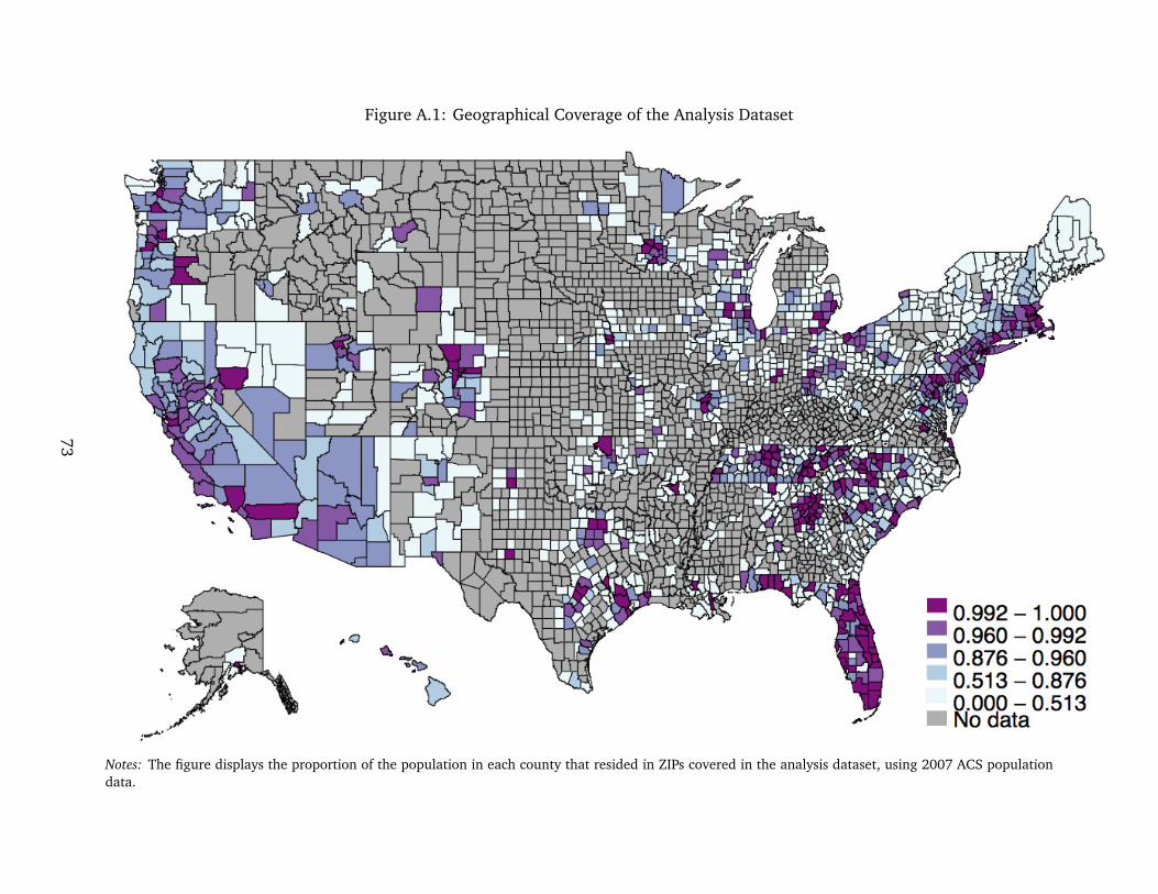
Figure A.1: Geographical Coverage of the Analysis Dataset

Notes: The figure displays the proportion of the population in each county that resided in ZIPs covered in the analysis dataset, using 2007 ACS populationdata.

73

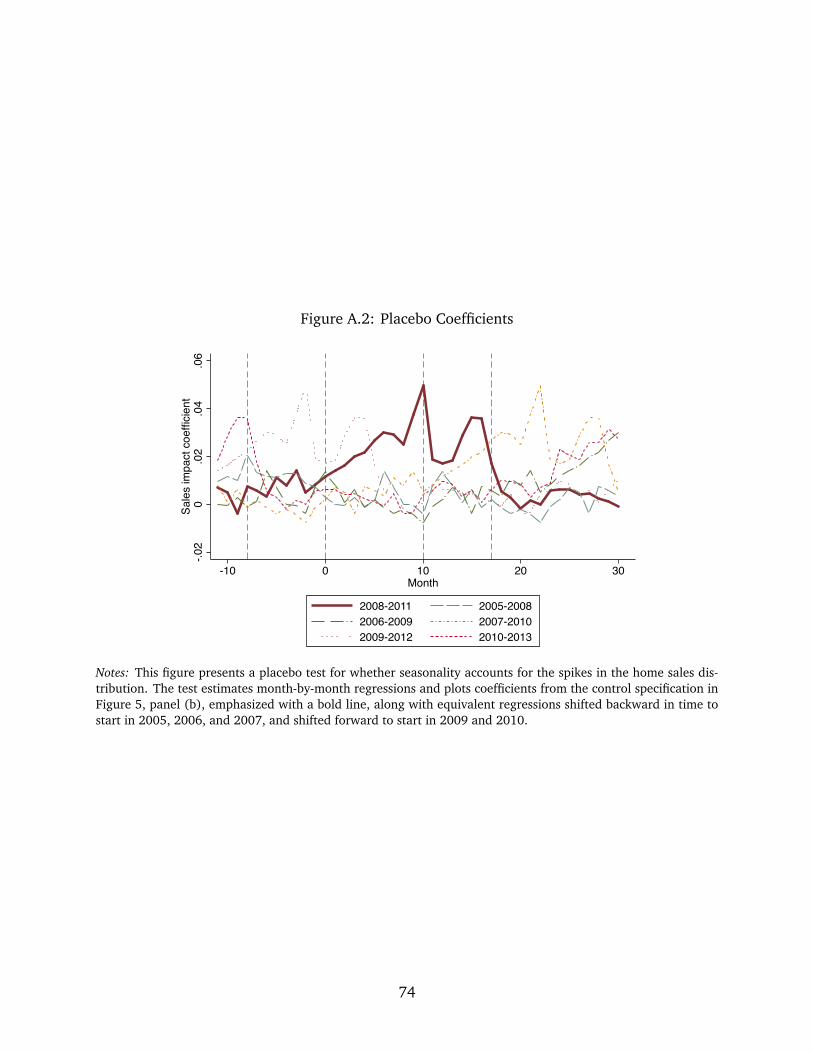
Figure A.2: Placebo Coefficients

-.02

0.0

2.0

4.0

6Sa

les

impa

ct c

oeffi

cien

t

-10 0 10 20 30Month

2008-2011 2005-20082006-2009 2007-20102009-2012 2010-2013

Notes: This figure presents a placebo test for whether seasonality accounts for the spikes in the home sales dis-tribution. The test estimates month-by-month regressions and plots coefficients from the control specification inFigure 5, panel (b), emphasized with a bold line, along with equivalent regressions shifted backward in time tostart in 2005, 2006, and 2007, and shifted forward to start in 2009 and 2010.

74

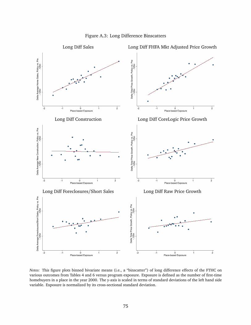
Figure A.3: Long Difference Binscatters

Long Diff Sales Long Diff FHFA Mkt Adjusted Price Growth

-.125

σ.1

25σ

Del

ta A

vera

ge H

ome

Sale

s, P

olic

y vs

. Pre

-2 -1 0 1 2Place-based Exposure

-.125

σ.1

25σ

Del

ta T

otal

Pric

e G

row

th, P

olic

y vs

. Pre

-2 -1 0 1 2Place-based Exposure

Long Diff Construction Long Diff CoreLogic Price Growth

-.125

σ.1

25σ

Del

ta A

vera

ge N

ew C

onst

ruct

ion,

Pol

icy

vs. P

re

-2 -1 0 1 2Place-based Exposure

-.125

σ.1

25σ

Del

ta T

otal

Pric

e G

row

th, P

olic

y vs

. Pre

-2 -1 0 1 2Place-based Exposure

Long Diff Foreclosures/Short Sales Long Diff Raw Price Growth

-.125

σ.1

25σ

Del

ta A

vera

ge F

orec

losu

res/

Shor

t Sal

es, P

olic

y vs

. Pre

-2 -1 0 1 2Place-based Exposure

-.125

σ.1

25σ

Del

ta T

otal

Pric

e G

row

th, P

olic

y vs

. Pre

-2 -1 0 1 2Place-based Exposure

Notes: This figure plots binned bivariate means (i.e., a “binscatter”) of long difference effects of the FTHC onvarious outcomes from Tables 4 and 6 versus program exposure. Exposure is defined as the number of first-timehomebuyers in a place in the year 2000. The y-axis is scaled in terms of standard deviations of the left hand sidevariable. Exposure is normalized by its cross-sectional standard deviation.

75

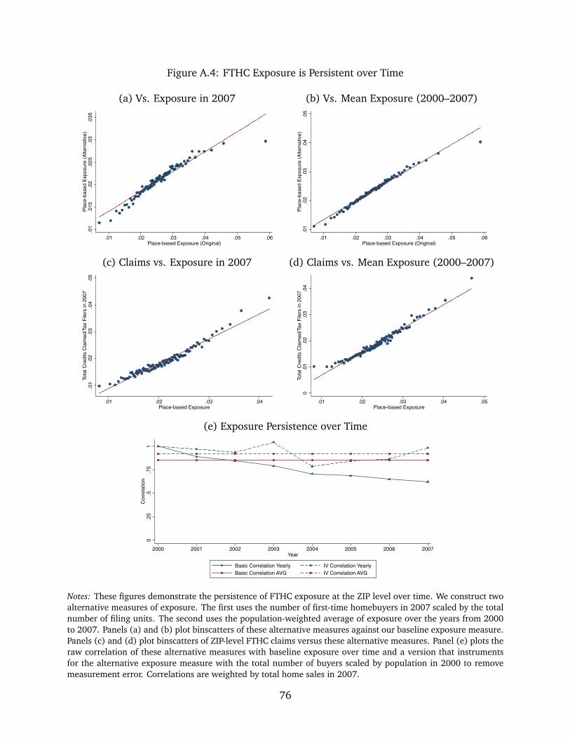
Figure A.4: FTHC Exposure is Persistent over Time

(a) Vs. Exposure in 2007 (b) Vs. Mean Exposure (2000–2007).0

1.0

15.0

2.0

25.0

3.0

35Pl

ace-

base

d Ex

posu

re (A

ltern

ative

)

.01 .02 .03 .04 .05 .06Place-based Exposure (Original)

.01

.02

.03

.04

.05

Plac

e-ba

sed

Expo

sure

(Alte

rnat

ive)

.01 .02 .03 .04 .05 .06Place-based Exposure (Original)

(c) Claims vs. Exposure in 2007 (d) Claims vs. Mean Exposure (2000–2007)

.01

.02

.03

.04

.05

Tota

l Cre

dits

Cla

imed

/Tax

File

rs in

200

7

.01 .02 .03 .04Place-based Exposure

0.0

1.0

2.0

3.0

4To

tal C

redi

ts C

laim

ed/T

ax F

ilers

in 2

007

.01 .02 .03 .04 .05Place-based Exposure

(e) Exposure Persistence over Time

0.2

5.5

.75

1C

orre

latio

n

2000 2001 2002 2003 2004 2005 2006 2007Year

Basic Correlation Yearly IV Correlation YearlyBasic Correlation AVG IV Correlation AVG

Notes: These figures demonstrate the persistence of FTHC exposure at the ZIP level over time. We construct twoalternative measures of exposure. The first uses the number of first-time homebuyers in 2007 scaled by the totalnumber of filing units. The second uses the population-weighted average of exposure over the years from 2000to 2007. Panels (a) and (b) plot binscatters of these alternative measures against our baseline exposure measure.Panels (c) and (d) plot binscatters of ZIP-level FTHC claims versus these alternative measures. Panel (e) plots theraw correlation of these alternative measures with baseline exposure over time and a version that instrumentsfor the alternative exposure measure with the total number of buyers scaled by population in 2000 to removemeasurement error. Correlations are weighted by total home sales in 2007.

76

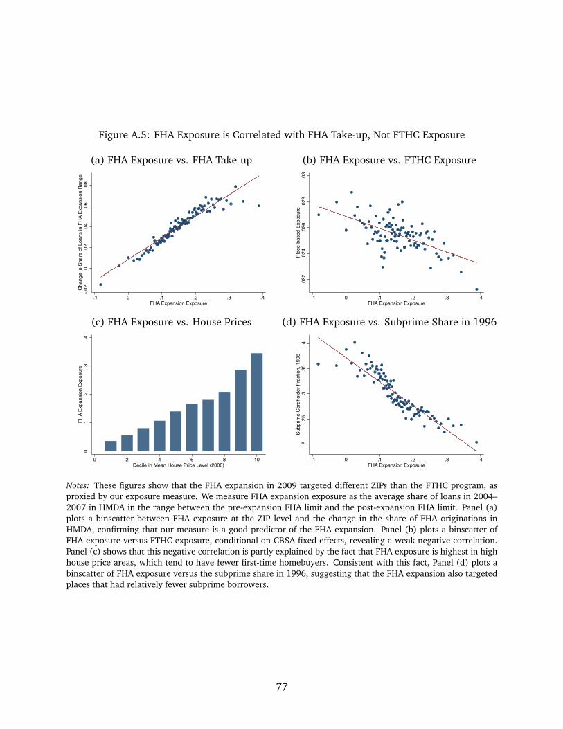
Figure A.5: FHA Exposure is Correlated with FHA Take-up, Not FTHC Exposure

(a) FHA Exposure vs. FHA Take-up (b) FHA Exposure vs. FTHC Exposure

-.02

0.0

2.0

4.0

6.0

8C

hang

e in

Sha

re o

f Loa

ns in

FH

A Ex

pans

ion

Ran

ge

-.1 0 .1 .2 .3 .4FHA Expansion Exposure

.022

.024

.026

.028

.03

Plac

e-ba

sed

Expo

sure

-.1 0 .1 .2 .3 .4FHA Expansion Exposure

(c) FHA Exposure vs. House Prices (d) FHA Exposure vs. Subprime Share in 1996

0.1

.2.3

.4FH

A Ex

pans

ion

Expo

sure

0 2 4 6 8 10Decile in Mean House Price Level (2008)

.2.2

5.3

.35

.4Su

bprim

e C

ardh

olde

r Fra

ctio

n, 1

996

-.1 0 .1 .2 .3 .4FHA Expansion Exposure

Notes: These figures show that the FHA expansion in 2009 targeted different ZIPs than the FTHC program, asproxied by our exposure measure. We measure FHA expansion exposure as the average share of loans in 2004–2007 in HMDA in the range between the pre-expansion FHA limit and the post-expansion FHA limit. Panel (a)plots a binscatter between FHA exposure at the ZIP level and the change in the share of FHA originations inHMDA, confirming that our measure is a good predictor of the FHA expansion. Panel (b) plots a binscatter ofFHA exposure versus FTHC exposure, conditional on CBSA fixed effects, revealing a weak negative correlation.Panel (c) shows that this negative correlation is partly explained by the fact that FHA exposure is highest in highhouse price areas, which tend to have fewer first-time homebuyers. Consistent with this fact, Panel (d) plots abinscatter of FHA exposure versus the subprime share in 1996, suggesting that the FHA expansion also targetedplaces that had relatively fewer subprime borrowers.

77

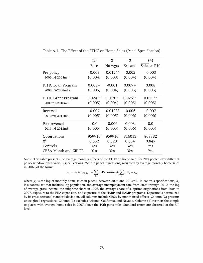
Table A.1: The Effect of the FTHC on Home Sales (Panel Specification)

(1) (2) (3) (4)Base No wgts Ex sand Sales> P10

Pre-policy -0.003 -0.012** -0.002 -0.0032006m4-2008m4 (0.004) (0.003) (0.004) (0.004)

FTHC Loan Program 0.008+ -0.001 0.009+ 0.0082008m5-2008m12 (0.005) (0.004) (0.005) (0.005)

FTHC Grant Program 0.024** 0.018** 0.026** 0.025**2009m1-2010m5 (0.005) (0.004) (0.005) (0.005)

Reversal -0.007 -0.012** -0.006 -0.0072010m6-2011m5 (0.005) (0.005) (0.006) (0.006)

Post-reversal -0.0 -0.006 0.003 0.02011m6-2013m5 (0.005) (0.005) (0.006) (0.005)

Observations 959916 959916 816013 868382R2 0.852 0.828 0.854 0.847Controls Yes Yes Yes YesCBSA-Month and ZIP FE Yes Yes Yes Yes

Notes: This table presents the average monthly effects of the FTHC on home sales for ZIPs pooled over differentpolicy windows with various specifications. We run panel regressions, weighted by average monthly home salesin 2007, of the form:

yi t = αi +δCBSA,t +∑

P

βPExposurei +∑

t

γt X i + εi t

where yi is the log of monthly home sales in place i between 2004 and 2013m5. In controls specifications, X iis a control set that includes log population, the average unemployment rate from 2006 through 2010, the logof average gross income, the subprime share in 1996, the average share of subprime originations from 2004 to2007, exposure to the FHA expansion, and exposure to the HARP and HAMP programs. Exposure is normalizedby its cross-sectional standard deviation. All columns include CBSA-by-month fixed effects. Column (2) presentsunweighted regressions. Column (3) excludes Arizona, California, and Nevada. Column (4) restricts the sampleto places with average home sales in 2007 above the 10th percentile. Standard errors are clustered at the ZIPlevel.

78

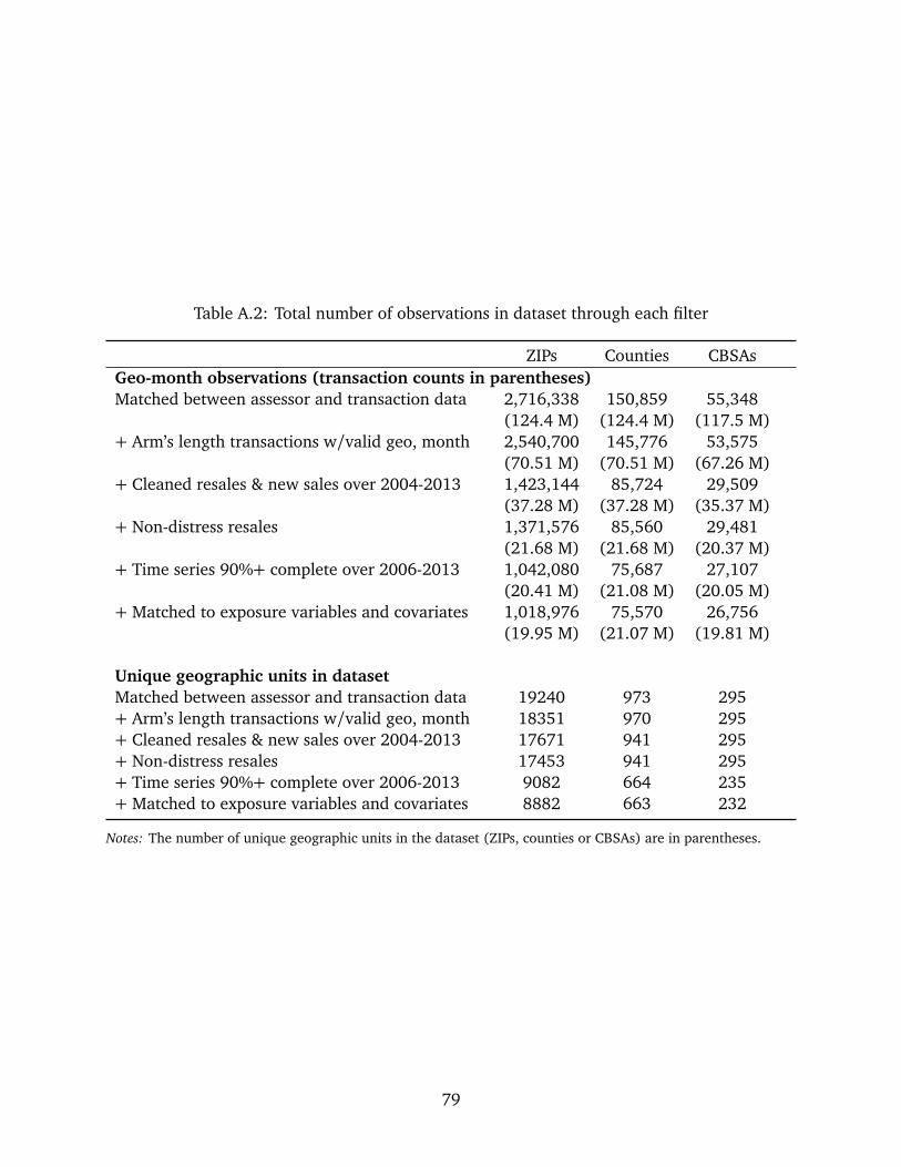
Table A.2: Total number of observations in dataset through each filter

ZIPs Counties CBSAsGeo-month observations (transaction counts in parentheses)Matched between assessor and transaction data 2,716,338 150,859 55,348

(124.4 M) (124.4 M) (117.5 M)+ Arm’s length transactions w/valid geo, month 2,540,700 145,776 53,575

(70.51 M) (70.51 M) (67.26 M)+ Cleaned resales & new sales over 2004-2013 1,423,144 85,724 29,509

(37.28 M) (37.28 M) (35.37 M)+ Non-distress resales 1,371,576 85,560 29,481

(21.68 M) (21.68 M) (20.37 M)+ Time series 90%+ complete over 2006-2013 1,042,080 75,687 27,107

(20.41 M) (21.08 M) (20.05 M)+ Matched to exposure variables and covariates 1,018,976 75,570 26,756

(19.95 M) (21.07 M) (19.81 M)

Unique geographic units in datasetMatched between assessor and transaction data 19240 973 295+ Arm’s length transactions w/valid geo, month 18351 970 295+ Cleaned resales & new sales over 2004-2013 17671 941 295+ Non-distress resales 17453 941 295+ Time series 90%+ complete over 2006-2013 9082 664 235+ Matched to exposure variables and covariates 8882 663 232

Notes: The number of unique geographic units in the dataset (ZIPs, counties or CBSAs) are in parentheses.

79

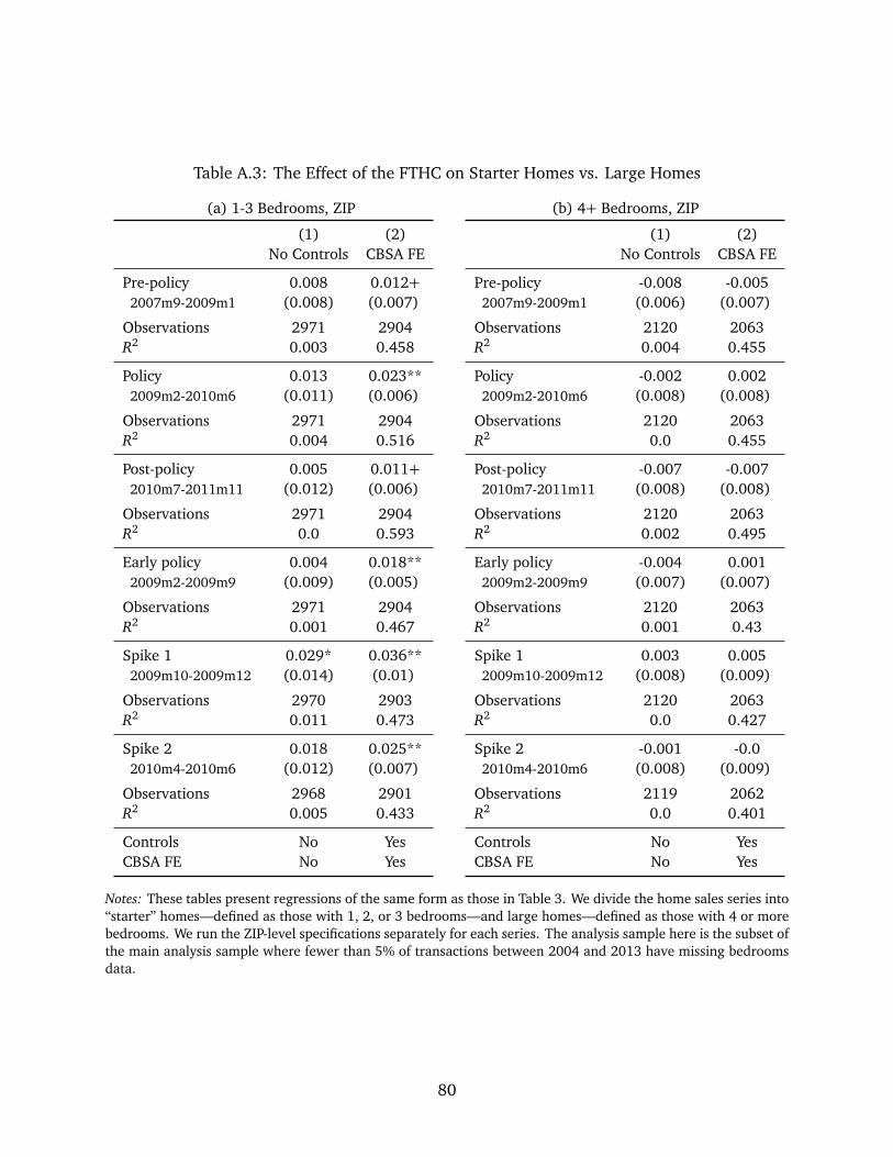
Table A.3: The Effect of the FTHC on Starter Homes vs. Large Homes

(a) 1-3 Bedrooms, ZIP (b) 4+ Bedrooms, ZIP

(1) (2)No Controls CBSA FE

Pre-policy 0.008 0.012+2007m9-2009m1 (0.008) (0.007)

Observations 2971 2904R2 0.003 0.458

Policy 0.013 0.023**2009m2-2010m6 (0.011) (0.006)

Observations 2971 2904R2 0.004 0.516

Post-policy 0.005 0.011+2010m7-2011m11 (0.012) (0.006)

Observations 2971 2904R2 0.0 0.593

Early policy 0.004 0.018**2009m2-2009m9 (0.009) (0.005)

Observations 2971 2904R2 0.001 0.467

Spike 1 0.029* 0.036**2009m10-2009m12 (0.014) (0.01)

Observations 2970 2903R2 0.011 0.473

Spike 2 0.018 0.025**2010m4-2010m6 (0.012) (0.007)

Observations 2968 2901R2 0.005 0.433

Controls No YesCBSA FE No Yes

(1) (2)No Controls CBSA FE

Pre-policy -0.008 -0.0052007m9-2009m1 (0.006) (0.007)

Observations 2120 2063R2 0.004 0.455

Policy -0.002 0.0022009m2-2010m6 (0.008) (0.008)

Observations 2120 2063R2 0.0 0.455

Post-policy -0.007 -0.0072010m7-2011m11 (0.008) (0.008)

Observations 2120 2063R2 0.002 0.495

Early policy -0.004 0.0012009m2-2009m9 (0.007) (0.007)

Observations 2120 2063R2 0.001 0.43

Spike 1 0.003 0.0052009m10-2009m12 (0.008) (0.009)

Observations 2120 2063R2 0.0 0.427

Spike 2 -0.001 -0.02010m4-2010m6 (0.008) (0.009)

Observations 2119 2062R2 0.0 0.401

Controls No YesCBSA FE No Yes

Notes: These tables present regressions of the same form as those in Table 3. We divide the home sales series into“starter” homes—defined as those with 1, 2, or 3 bedrooms—and large homes—defined as those with 4 or morebedrooms. We run the ZIP-level specifications separately for each series. The analysis sample here is the subset ofthe main analysis sample where fewer than 5% of transactions between 2004 and 2013 have missing bedroomsdata.

80

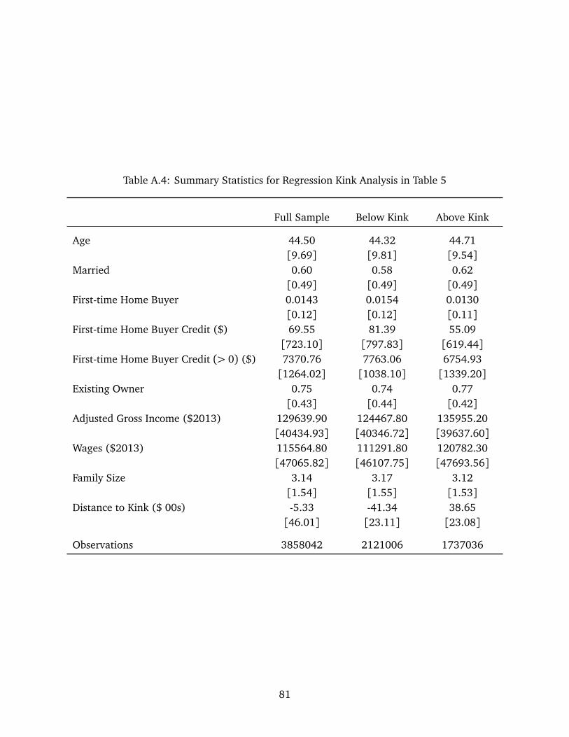
Table A.4: Summary Statistics for Regression Kink Analysis in Table 5

Full Sample Below Kink Above Kink

Age 44.50 44.32 44.71[9.69] [9.81] [9.54]

Married 0.60 0.58 0.62[0.49] [0.49] [0.49]

First-time Home Buyer 0.0143 0.0154 0.0130[0.12] [0.12] [0.11]

First-time Home Buyer Credit ($) 69.55 81.39 55.09[723.10] [797.83] [619.44]

First-time Home Buyer Credit (> 0) ($) 7370.76 7763.06 6754.93[1264.02] [1038.10] [1339.20]

Existing Owner 0.75 0.74 0.77[0.43] [0.44] [0.42]

Adjusted Gross Income ($2013) 129639.90 124467.80 135955.20[40434.93] [40346.72] [39637.60]

Wages ($2013) 115564.80 111291.80 120782.30[47065.82] [46107.75] [47693.56]

Family Size 3.14 3.17 3.12[1.54] [1.55] [1.53]

Distance to Kink ($ 00s) -5.33 -41.34 38.65[46.01] [23.11] [23.08]

Observations 3858042 2121006 1737036

81

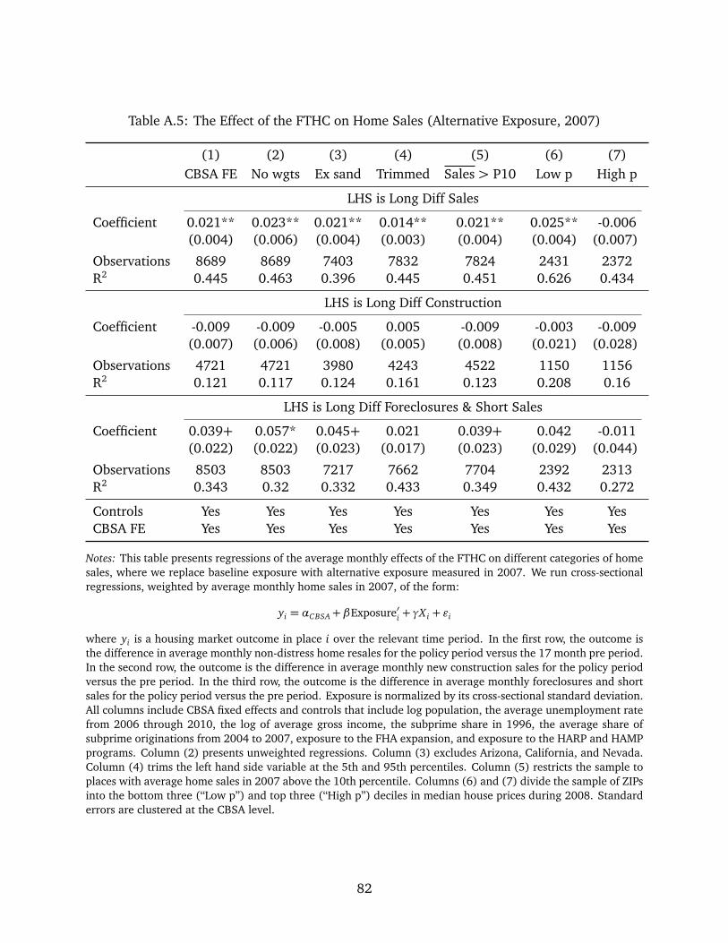
Table A.5: The Effect of the FTHC on Home Sales (Alternative Exposure, 2007)

(1) (2) (3) (4) (5) (6) (7)CBSA FE No wgts Ex sand Trimmed Sales > P10 Low p High p

LHS is Long Diff Sales

Coefficient 0.021** 0.023** 0.021** 0.014** 0.021** 0.025** -0.006(0.004) (0.006) (0.004) (0.003) (0.004) (0.004) (0.007)

Observations 8689 8689 7403 7832 7824 2431 2372R2 0.445 0.463 0.396 0.445 0.451 0.626 0.434

LHS is Long Diff Construction

Coefficient -0.009 -0.009 -0.005 0.005 -0.009 -0.003 -0.009(0.007) (0.006) (0.008) (0.005) (0.008) (0.021) (0.028)

Observations 4721 4721 3980 4243 4522 1150 1156R2 0.121 0.117 0.124 0.161 0.123 0.208 0.16

LHS is Long Diff Foreclosures & Short Sales

Coefficient 0.039+ 0.057* 0.045+ 0.021 0.039+ 0.042 -0.011(0.022) (0.022) (0.023) (0.017) (0.023) (0.029) (0.044)

Observations 8503 8503 7217 7662 7704 2392 2313R2 0.343 0.32 0.332 0.433 0.349 0.432 0.272

Controls Yes Yes Yes Yes Yes Yes YesCBSA FE Yes Yes Yes Yes Yes Yes Yes

Notes: This table presents regressions of the average monthly effects of the FTHC on different categories of homesales, where we replace baseline exposure with alternative exposure measured in 2007. We run cross-sectionalregressions, weighted by average monthly home sales in 2007, of the form:

yi = αCBSA+ βExposure′i + γX i + εi

where yi is a housing market outcome in place i over the relevant time period. In the first row, the outcome isthe difference in average monthly non-distress home resales for the policy period versus the 17 month pre period.In the second row, the outcome is the difference in average monthly new construction sales for the policy periodversus the pre period. In the third row, the outcome is the difference in average monthly foreclosures and shortsales for the policy period versus the pre period. Exposure is normalized by its cross-sectional standard deviation.All columns include CBSA fixed effects and controls that include log population, the average unemployment ratefrom 2006 through 2010, the log of average gross income, the subprime share in 1996, the average share ofsubprime originations from 2004 to 2007, exposure to the FHA expansion, and exposure to the HARP and HAMPprograms. Column (2) presents unweighted regressions. Column (3) excludes Arizona, California, and Nevada.Column (4) trims the left hand side variable at the 5th and 95th percentiles. Column (5) restricts the sample toplaces with average home sales in 2007 above the 10th percentile. Columns (6) and (7) divide the sample of ZIPsinto the bottom three (“Low p”) and top three (“High p”) deciles in median house prices during 2008. Standarderrors are clustered at the CBSA level.

82

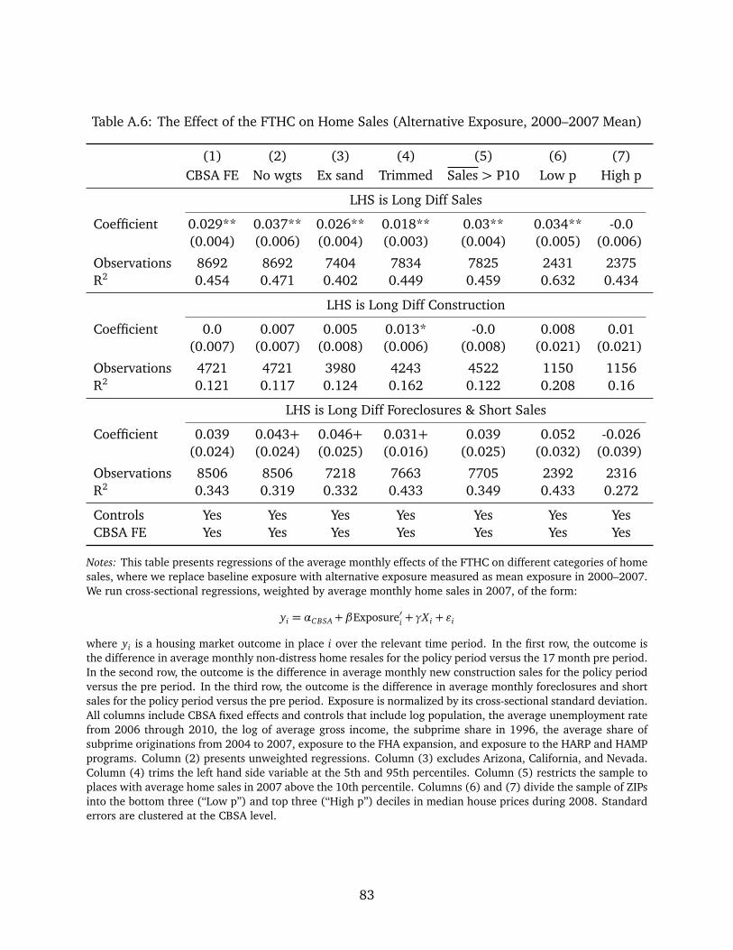
Table A.6: The Effect of the FTHC on Home Sales (Alternative Exposure, 2000–2007 Mean)

(1) (2) (3) (4) (5) (6) (7)CBSA FE No wgts Ex sand Trimmed Sales > P10 Low p High p

LHS is Long Diff Sales

Coefficient 0.029** 0.037** 0.026** 0.018** 0.03** 0.034** -0.0(0.004) (0.006) (0.004) (0.003) (0.004) (0.005) (0.006)

Observations 8692 8692 7404 7834 7825 2431 2375R2 0.454 0.471 0.402 0.449 0.459 0.632 0.434

LHS is Long Diff Construction

Coefficient 0.0 0.007 0.005 0.013* -0.0 0.008 0.01(0.007) (0.007) (0.008) (0.006) (0.008) (0.021) (0.021)

Observations 4721 4721 3980 4243 4522 1150 1156R2 0.121 0.117 0.124 0.162 0.122 0.208 0.16

LHS is Long Diff Foreclosures & Short Sales

Coefficient 0.039 0.043+ 0.046+ 0.031+ 0.039 0.052 -0.026(0.024) (0.024) (0.025) (0.016) (0.025) (0.032) (0.039)

Observations 8506 8506 7218 7663 7705 2392 2316R2 0.343 0.319 0.332 0.433 0.349 0.433 0.272

Controls Yes Yes Yes Yes Yes Yes YesCBSA FE Yes Yes Yes Yes Yes Yes Yes

Notes: This table presents regressions of the average monthly effects of the FTHC on different categories of homesales, where we replace baseline exposure with alternative exposure measured as mean exposure in 2000–2007.We run cross-sectional regressions, weighted by average monthly home sales in 2007, of the form:

yi = αCBSA+ βExposure′i + γX i + εi

where yi is a housing market outcome in place i over the relevant time period. In the first row, the outcome isthe difference in average monthly non-distress home resales for the policy period versus the 17 month pre period.In the second row, the outcome is the difference in average monthly new construction sales for the policy periodversus the pre period. In the third row, the outcome is the difference in average monthly foreclosures and shortsales for the policy period versus the pre period. Exposure is normalized by its cross-sectional standard deviation.All columns include CBSA fixed effects and controls that include log population, the average unemployment ratefrom 2006 through 2010, the log of average gross income, the subprime share in 1996, the average share ofsubprime originations from 2004 to 2007, exposure to the FHA expansion, and exposure to the HARP and HAMPprograms. Column (2) presents unweighted regressions. Column (3) excludes Arizona, California, and Nevada.Column (4) trims the left hand side variable at the 5th and 95th percentiles. Column (5) restricts the sample toplaces with average home sales in 2007 above the 10th percentile. Columns (6) and (7) divide the sample of ZIPsinto the bottom three (“Low p”) and top three (“High p”) deciles in median house prices during 2008. Standarderrors are clustered at the CBSA level.

83