Evaluation of Photographic Properties for Area Estlmation

bvSteven Jay Wiles

May, 1988

Blacksburg, Virginia

l

Evaluation of Photographic Properties for Area Estimation

bvSteven Jay Wiles

James L. Smith, Chairman

Forestry

(ABSTRACT)

From the known image positional errors on aerial photographs, this thesis computes and

evaluates acreage estimation errors. Four hypothetical tracts were used in simulating aerial

photographs with 104 different camera orientation combinations. Flying heights of 4000 and

6000 feet, focal Iengths of 24 and 50 millimeters with and without lens distortion, and tilts of

4- 0, 3, 6, and 12 degrees were simulated. The 416 photographs were all simulated with thewi

camera exposure station centered above the midpoint of the respective tract's bounding ree-X

tangle. The topographic relief of the tracts ranged from 19 feet in the Coastal Plain to 105 feet

~ in the Piedmont.R-lt was found that lens focal length did not have an independent effect on the acreage esti-

mates. Relief error, the lowest, averaged -0.080%. ln comparison, small errors in calculating

scale were shown to be larger than relief errors. Tilt was recommended to be limited to six

degrees, averaging +1.6% error at six degrees tilt. Because of its positive exponential nature

when the tracts are centered, tilt can induce large biases. including tilts from zero to six de-

grees, the average was 0.634%. Lens distortion error averaged -0.686%. Overall, the aver-

age acreage error was 0.363% for simulations up to and including six degrees of tilt with and

without lens distortion. This result is for centered tracts, and it was felt many of the errors

were compensating given this situation. In conclusion, the photographie images can estimate

areas to $1%, however, additional errors are imparted during actual measurement of the

photographs.

Acknowledgements

Acknowledgements iii

l S S

I

Table of Contents

INTRODUCTION ......................................................... 1

LITERATURE REVIEW .................................................... 3

ADVANTAGES AND DISADVANTAGES OF 35-MM .............................. 3

APPLICATIONS OF 35-MM ............................................... 6

QUALITATIVE APPLICATIONS ........................................... 6

QUANTITATIVE APPLICATIONS .......................................... 8

LOCATION ERROR IN PHOTOGRAPHIC IMAGE .............................. 12

RELIEF .............................................,............. 12

TILT ............................................................. 15

EQUIPMENT ....................................................,.. 17

SUMMARY .......................................................... 20

MATERIALS AND METHODS .............................................. 21

DATA COLLECTION ................................................... 22

PHOTOGRAPHIC SIMULATION ........................................... 23

METHODS OF ANALYSIS ............................................... 26

Table of Contents iv

I

III

COMPUTER PROGRAMS ............................................... 28

RESULTS AND DISCUSSION .............................................. 31RELIEF ............................................................. 36CAMERA TI LT ....................................................... 51LENS DISTORTION .................................................... 57

SUMMARY AND CONCLUSION ............................................ 63

BIBLIOGRAPHY ........................................................ 67

Appendlx A. MAPPER ................................................... 69

Appendix B. ACREAGE .................................................. 72

Appendix C. PHOTOSIM ................................................. 79

Appendix D. SLIDE ..................................................... 92

VITA ............................................................... 100

Table of Contents v

l1

List of lllustrations

Figure 1. Drawing of relief displacement. ................................... 13

Figure 2. Displacement error at various flying heights and difference in topographic relief 14

Figure 3. Drawing of tilt displacement. ..................................... 16

Figure 4. Curves showing error in horizontal position caused by tilt ............... 18

Figure 5. Example of lens distortion curve for 35·mm camera .................... 25

Figure 6. Topography of Crewe West, VA. area. .............................. 37

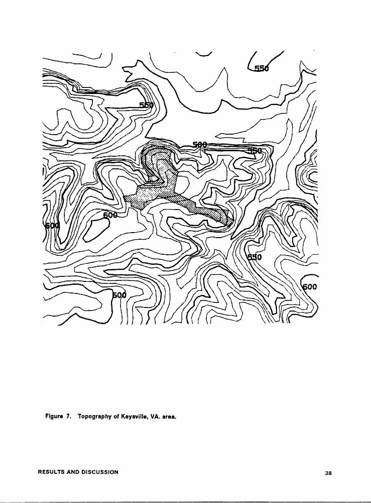
Figure 7. Topography of Keysville, VA. area. ................................. 38

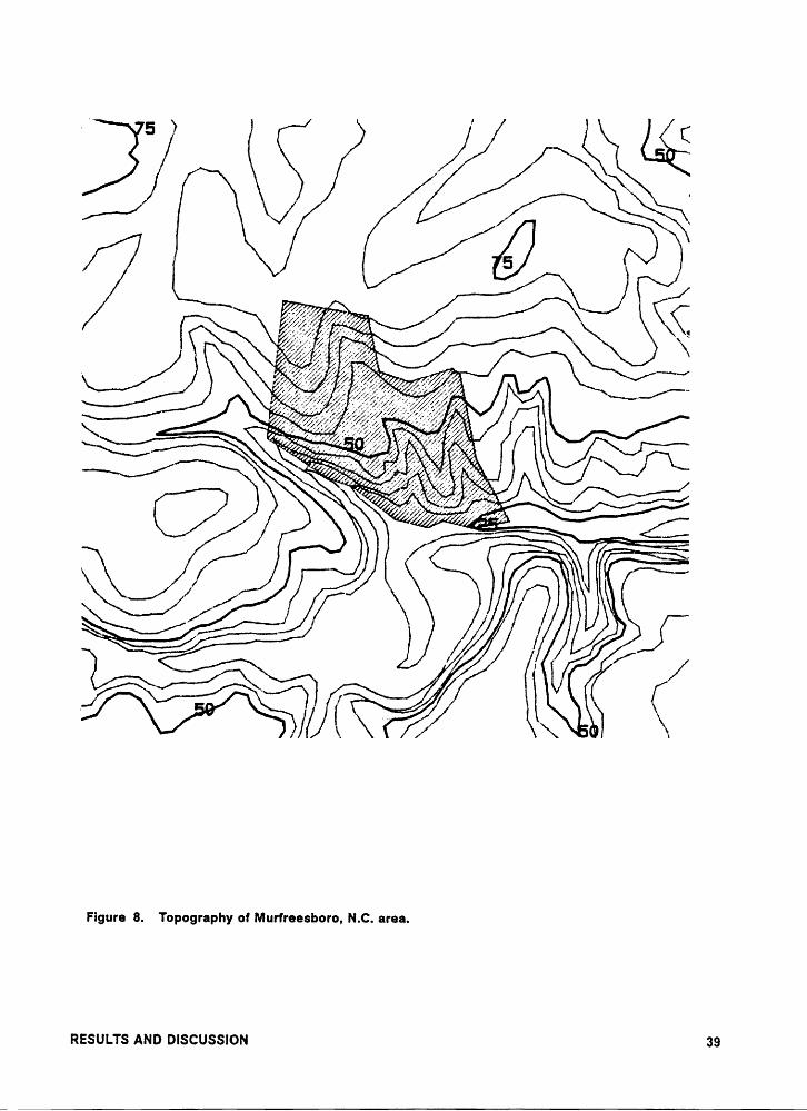
Figure 8. Topography of Murfreesboro, N.C. area. ............................. 39

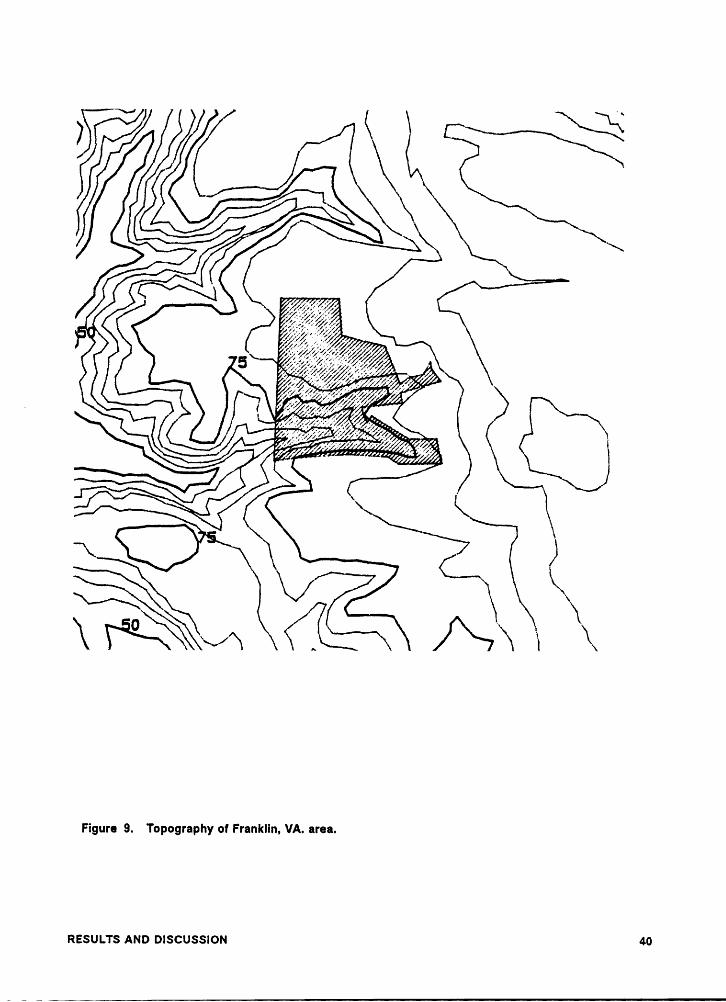
Figure 9. Topography of Franklin, VA. area. ................................. 40

Figure 10. Franklin tract with and without relief displacement. .................... 45

Figure 11. Crewe West tract with and without relief displacement. ................. 46

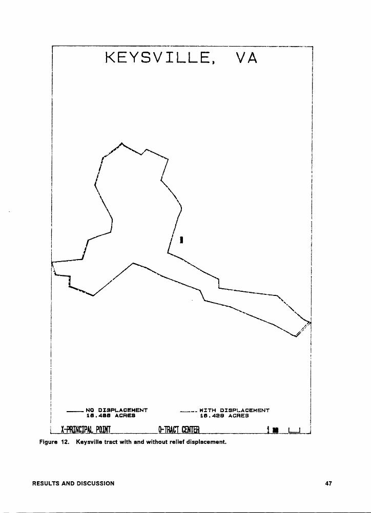
Figure 12. Keysville tract with and without relief displacement. ................... 47

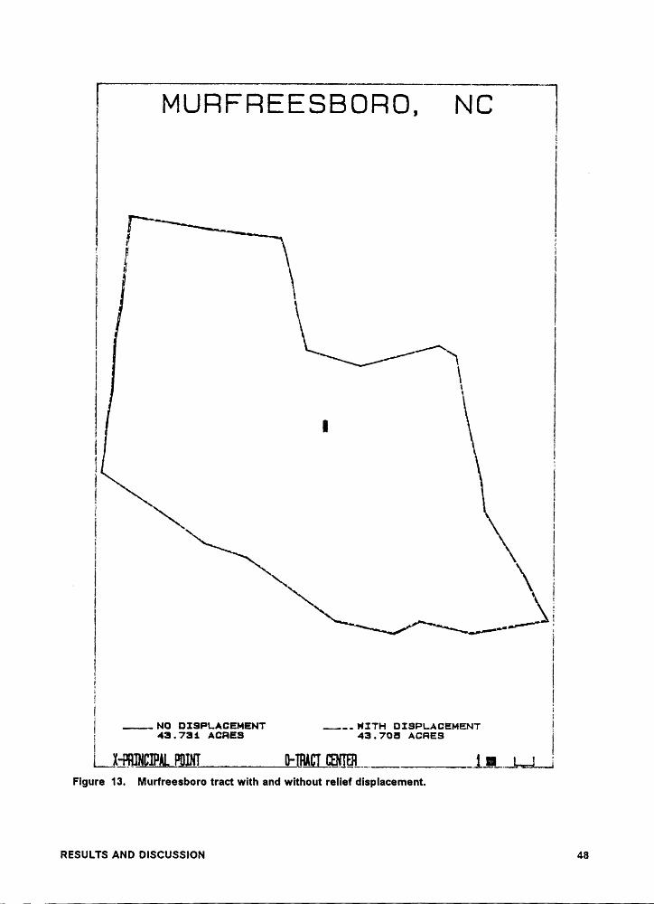
Figure 13. Murfreesboro tract with and without relief displacement. ................ 48

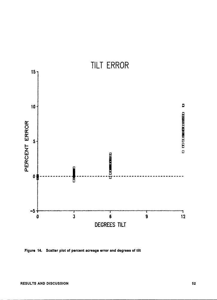
Figure 14. Scatter plot of percent acreage error and degrees of tilt ................ 52

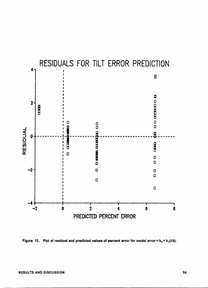
Figure 15. Plot of residual and predicted values of percent error for modelerror= bo + b,(tilt). ............................................. 54

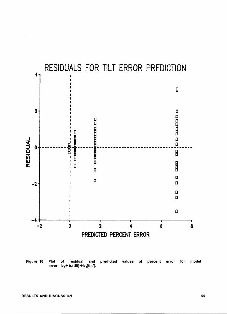
Figure 16. Plot of residual and predicted values of percent error for modelerror= bo + b1(tilt)+ b,(tilt“). ...................................... 55

Figure 17. Graph of percent error for circles with lens distortion. .................. 61

Figure 18. Plot of true Keysville tract overlain with photograph at 4000ft, 50mm, and 6 de-gree tilt east, with lens distortion. ................................. 64

List ¤i iiuusuazaens vi

List of Tables

Table 1. Difference between the actual location and photogrammetric location of testtargets. ...................................................... 10

Table 2. Results ofthe simulations for Crewe West, V.A. ....................... 32

Table 3. Results of the simulations for Franklin, V.A. ........................... 33

Table 4. Results ofthe simulations for Keysville, V.A. .......................... 34

Table 5. Results of the simulations for Murfreesboro, N.C. ...................... 35

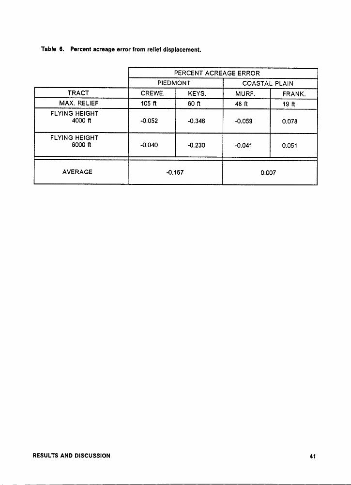
Table 6. Percent acreage error from relief displacement. ....................... 41

Table 7. Effect flying height error has on percent acreage error, 4000ft and 6000ft are usedin calculating respective tract acres. ............................... 43

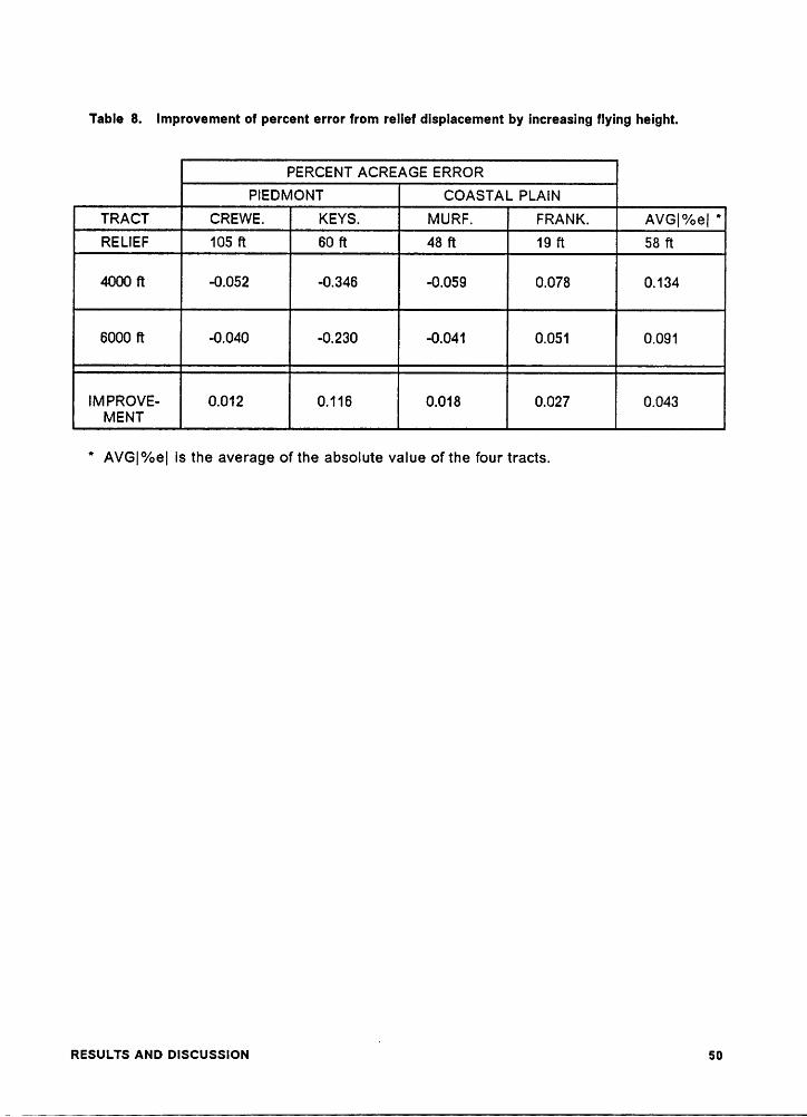
Table 8. Improvement of percent error from relief displacement by increasing flyingheight. ...................................................... 50

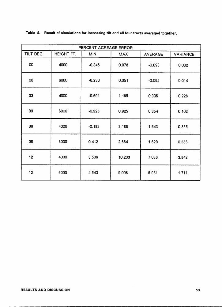
Table 9. Result of simulations for increasing tilt and all four tracts averaged together. . 53

Table 10. Average of change in percent error for with and without lens distortion averagedover all tilts and repetitions ...................................... 59

Table 11. Average of change in percent error for with and without lens distortion for tiltsof0 to 6 degrees. .............................................. 62

List of Tables vll

ll

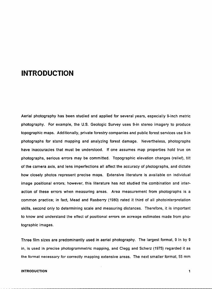
INTRODUCTION

Aerial photography has been studied and applied for several years, especially 9-inch metric

photography. For example, the U.S. Geologic Survey uses 9-in stereo imagery to produce

topographic maps. Additionally, private forestry companies and public forest services use 9-in

photographs for stand mapping and analyzing forest damage. Nevertheless, photographs

have inaccuracies that must be understood. lf one assumes map properties hold true on

photographs, serious errors may be committed. Topographic elevation changes (relief), tilt

of the camera axis, and lens imperfections all affect the accuracy of photographs, and dictate

how closely photos represent precise maps. Extensive literature is available on individual

image positional errors; however, this literature has not studied the combination and inter-

action of these errors when measuring areas. Area measurement from photographs is a

common practice; in fact, Mead and Rasberry (1980) rated it third of all photointerpretation

skills, second only to determining scale and measuring distances. Therefore, it is important

to know and understand the effect of positional errors on acreage estimates made from pho-

tographic images.

Three film sizes are predominantly used in aerial photography. The largest format, 9 in by 9

in, is used in precise photogrammetric mapping, and Clegg and Scherz (1975) regarded it as

the format necessary for correctly mapping e><tensive areas. The ne><t smaller format, 55 mm

lNTRoDUcTloNn

1

by 55 mm, is used in Canada for forest inventory and tree identification. By integrating the

70-mm camera system with radar altimeters and tilt indicators, the results were within desired

accuracy limits (Meyer 1982). The smallest commonly used format, 36 mm by 24 mm, is a

relatively simple, lnexpensive, and fiexible system. For this reason, 35-mm systems are be-

ginning to be used more often on smaller projects. This 35-mm format has the least opera-

tional and initial investment costs, can be used with various camera mounts, and designed to

increase the professional capabilities of the field resource manager (Meyer and Grumstrup

1978). Even though it was reported as having the worst metric accuracy (Dalman 1978), only

limited research has evaluated these inaccuracies and their impact on management deci-

sions. In fact, although much is known about the errors of a single point on all of the formats,

no literature was available analyzing the accumulation and combination of these point errors

when calculating areas.

The objective of this project was motivated from the lack of knowledge on the accuracy of area

estimates from aerial photography. Focusing on 35-mm (the assumed worst case), the results

of this study will be applicable to the other more accurate formats. Specifically, the objective

of this study was to evaluate and compare the individual and combined effects of topographic

displacement, camera tilt, and lens distortion upon the accuracy and precision of area esti-

mates made on 35-mm aerial photographs.

lNTRo¤ucTloN 2

ä

LITERATURE REVIEW

ADVANTAGES AND DISADVANTAGES OF 35-MM

In comparison of the 9-in, 70-mm, and 35-mm formats, several authors have earnestly tried to

determine the appropriate niche for each format. These comparisons have evaluated many

aspects, a few of which are reiterated below to highlight the major points, and to provide a

basis for applying 35-mm to this study.

Speed and flexibility are strong advantages of 35-mm photography. Klein (1970) stated that

rapid, quality stereo images have been obtained with the 35-mm format. Addltionally, camera

systems with smaller formats are much simpler to use, and are adaptable to any type of alr-

craft which ls available at the time photography is needed (Spencer 1978). This flexibility

takes advantage of small openings in cloud cover to allow flying during the appropriate sea-

son (Meyer and Grumstrup 1978). Nine-inch camera systems require larger airplanes with

bellypan hole camera mounts, target viewing equipment, and integrated operating systems

permanently fastened in the aircralt. Seventy—milIimeter cameras are more flexible and can

be mounted in other locations on the aircraft. Thirty five-millimeter camera mounts range

from simply hand holding the camera, to constructed window mounts, and elaborate bellypan

LL LITERATURE REVIEW 3l

Imounts similar to those used with 9-in cameras. Most importantly, no modifications to the

airplane are required (Meyer and Grumstrup 1978). Furthermore, film acquisition and proc-

essing problems of the larger formats are alleviated by using normal color 35-mm film.

The cost of photographic systems can greatly influence which system is selected. The

equipment and film traditionally employed for mapping are expensive. Clegg and Scherz

(1975) compared the initial investment cost, and the cost for two photographs of the three

systems and found that for:

• 9-in cameras, the initial investment was $101,000, and the cost for two photos was $17.51;• 70-mm cameras, the initial investment was $7,500, and the cost for two photos was $2.85;• 35-mm cameras, the initial investment was $6,000, and the cost for two photos was $0.80.

Clegg and Scherz also noted that the cost of 9-in camera systems can run higherthan the cost

of an airplane. Both of the smaller formats were considerably less expensive than the 9-in

system, and furthermore, Roberts and Griswold (1986) found 35-mm to be twice as economical

as 70-mm. As a result of this lower cost, fiights for individual projects were feasible with

35-mm systems rather than compromising with general purpose photography (Roberts and

Griswold 1986). Although it ls obvious that 35-mm is less expensive per picture, one must also

consider how many pictures are necessary to cover the study area. Sixty 35-mm photos are

required to cover the equivalent of one 9-in photograph at the same scale (Spencer 1978), and,

150 photos are essential for stereo photography of an equal area covered by one 9-in stereo

pair (Roberts and Griswold 1986).

Besides greatly increasing the number of photographs, viewing and handling are two other

problems associated with the small format. To alleviate the viewing problem, size is in-

creased either by slide projection or enlargement with paper prints. Paper prints also help

solve the problem of handling small slides. Needham and Smith (1984) presented some ofthe

possible problems associated with paper prints including, decentering, loss of area due to

LlTERATuRE REVIEW 4

cropping, and loss of conjugate images. Furthermore, enlargement causes all light rays tol

pass through a second lens assembly subjecting them to additional distortions and displace-

ments.

Photographic resolution of the three formats was compared by Clegg and Scherz (1975). Se-

veral different sizes of targets were photographed at three elevations. They found that at fly-

ing heights of 1,000 feet, the smallest targets (1 ftz) were fuzzy on all formats. At heights of

3,000 feet, there was little difference between the 35-mm and the 70-mm formats, although

most of the targets on the 9-in format were one step sharper, and at 5,000 feet, the 9-in format

was superior. Additionally, Clegg and Scherz (1975) had two sets of experts, four in vegetation

and three in solls, compare the three formats. The vegetation experts all said the 35-mm

“provided good color rendition and resolution," and the four experts picked 35-mm as the

format they would use. The solls experts, on the other hand, preferred the 9-in format because

of the sharper resolution. However, when the pictures were concealed, so that the format was

unknown, the solls experts could not correctly pick the 9-in format from the others.

ln addition to photographic resolution, positional accuracy of an image is important. Accura-

cies of metric cameras approach 0.0001 times the flying height (Clegg and Scherz 1975). For

example, with a flying height of 1,000 feet, one can measure correct ground positions of an

object to within 0.1 foot, or approximately one inch. Clegg and Scherz (1975), in a comparison

of the three formats, published some surprising results about 35-mm accuracy. The study

measured 30 photo distances and compared these distances to a base map. The photographs

were rectifled in a tightly controlled area of 600 feet with a flying height of 5000 feet. 35-mm

had the least error of the three formats: 35-mm = 1.39%; 70-mm = 1.97%; 9-in = 1.77%.

To verify these results, a second test was conducted in which a scale factor was calculated

for 30 lines. Again, 35-mm came out with the least error: 35-mm = 1.49%; 70-mm = 2.02%;

9-in = 1.54%. A third test compared the positions of points outside of the tightly controlled

section and used the rectiüed 9-in photo as the base. Using four control points on the 9-in

photo, the smaller formats were rectiüed to match these four points. Using this procedure,

LITERATURE REVIEW 5

35·mm photography had an error of 11 feet, while 70-mm had an error of 6.5 feet. Since somel

users of 35·mm photography do not have expensive rectiüers, a standard 35·mm carousel

projector was then used. With this method Clegg and Scherz achieved accuracies of 8 feet

relative to ground positions calculated from the 9-in format. In another study, Roberts and

Griswold (1986) achieved accuracies of 0.0002 times flying height using 35-mm stereo imagery.

Both studies concluded that 35·mm photography was accurate enough for environmental

mapping which requires accuracies to tens of feet.

APPLICATIONS OF 35-MM

Numerous publications have been written on projects utilizing 35·mm aerial photography.

Klein (1970), Olson (1983), Miller and Meyer (1981), Shafer and Degler (1986), and Spencer

(1978) are some examples of applications from simple overviews to map generation. These

uses can be broken into two categories of qualitative and quantitative applications.

QUALITA TIVE APPLICA TIONS

Several authors have written about the advantages of small format aerial photography used

for general overviews without stringent mapping and measurement goals in mind. For ex-

ample, Shafer and Degler (1986) wrote, "When precise geographic positioning is not required

or when it can be obtained by correlating features on conventional photogrammetric images,

a great deal of data can be derived from hand—held photographs....Hand-held photography

offers the advantage of flexibility when qualitative, rather than quantitative, data are

required." 35-mm photography is often used in conjunction with preexisting maps, or older

9-in photography that are now out of date due to changes in the area. Duncan, Meyer, and

Moody (1984) found that National High Altitude Photography (NHAP) could estimate areas ac-

LITERATURE REVIEW 6

l

curately to 0.5 acres, but they needed supplemental 35-mm photography to get details of

specific areas.

Meyer (1982) presented several applications of small format photography used in conjunction

with preexisting photographs, one of which was the Minnesota forest peat lands survey. Black

and white 9-in resource photography of the 145,000 acres was available at a scale of 1:15,840,

but was inadequate for the task. Three levels of 35-mm color infrared photography furnished

the desired information at a reduced cost. Scales of 1:120,000, 1:80,000, and 1:11,000 were

fiown in two stages, and a third flight acquired low oblique photographs of difficult vegetation

boundaries. Meyer concluded, "Field verification in difficult classification areas indicated that

the basic resource photography, used in conjunction with the supplemental coverage, pro-

vided very good classification accuracy." (Meyer 1982)

Supplemental photographs have also been beneficial in identifying images on current

orthophotoquads. Mead and Gammon (1981) applied this technique for wetland vegetation

mapping of North Carolina. 35-mm color infrared photographs were used as a supplement to

recent 7.5 minute black and white USGS orthophotoquads. Only five percent of the area was

photographed at a scale of 1:6,000, yet all cover types were photographed because the flight

lines were keyed to high variation areas. The minimum mapping unit was four acres, in which

all species type boundaries were those as identltied on the orthophotoquad, and the supple-

mental aerial photographs were used only for type identification. Mead and Gammon con-

cluded through field checks that the results were acceptable.

Thirty-üve millimeter ülm has also been used as a primary source for qualitative information,

rather than used as a supplement to other sources of spatial data. Weih, Nord, and Meyer

(1982) evaluated film and filter combinations for 35-mm aerial photography at a scale of

1:20,000 to provide a low cost method for determining and mapping aspen regeneration

stocking levels. Aspen regeneration was separated into three classes, and stand maps were

then drawn using a rear projector screen. This allowed a more detailed analysis to be made

LITERATURE REVIEW 7

lof how harvesting methods affected regeneration. The photography also provided a perma- (

nent record of the stand for future use and management evaluation.

A fourth application of qualitative photography is tree identification. Needham (1983) used

large scale photos (1:650) to sample two forest stands during leaf change in the fall. Tree

presence and species were tallied for the sample plots on the ground for comparison to the

results of the photographs. The dominant and codominant trees could be identified with 95%

accuracy. Some of the factors affecting accuracy were tree spacing, whether or not a distlnct

image appeared on the photo, and dominance of the tree.

QUANTITA TIVE APPLICA TIONS

Quantitative applications of 35-mm photography do exist. However, a majority of the research

has been on qualitative applications, and several authors have stated that one must be cau-

tious in using 35-mm without metric control. For example, Dalman (1978) stated, "precision

measurements cannot be taken from 35-mm SAP (supplemental aerial photography) due to

distortions from: lens aberrations; displacement of objects on the photos; exaggeration of

heights; and an unlevel camera platform." Furthermore, Zsilinsky (1969) pointed out, "hand-

held photographs will generally not provide quantitative data except in gross terms. The

qualitative data that are easily collected, however, far surpass any disadvantages of lack of

control for mapping purposes." Quantitative uses can be divided into three areas, x,y posi-

tion, height, and area calculations. Image position, although not specifically stated, is proba-

bly the most important factor in any mapping or interpretation project. The accuracy at which

a system records images on film and subsequently projects and measures them is directly

correlated to the accuracy of the project’s results. The location of an object on a photo affects

the comparison of the identified object to the ground, measurement of distances between ob-

jects, and measurement of heights.

LITERATURE REVIEWe

8

One example of using single photo coordinates is measuring flame attributes. Clements, I

Ward, and Adkins (1983) used a 35-mm camera to measure flame height and distance of llre

line travel per unit time. Camera tilt created some unavoidable errors. Because tilt remains

constant for each picture, the ideal tilts for both height and distance calculations could not be

met at the same time. Flame height error is two percent at ten degrees tilt, and distance error

is six percent at twenty degrees tilt.

Goodrich (1982) conducted a study on the applicability of using terrestrial 35-mm stereo pho-

tography to monitor glacier movements. The analysis included tests of the camera and the

system. ln calibrating the camera, the side of a building was photographed with the test

camera and with a calibrated terrestrial camera. Window corners were then compared on

each picture to calibrate the 35-mm camera lens. Goodrich found the differences between the

actual location and photogrammetric location of test targets on the 35-mm picture to be ac-

curate enough for the application. The results, at distances of 100 and 200 feet, with and

without corrections for parallax from the camera calibration, are presented in Table 1

(Goodrich 1982). Goodrich concluded, "The results lndicate that a 35-mm camera can be used

in the system described for obtaining stereo pairs without fear of signiücant distortion errors

being introduced by the camera." Stereo pairs analyzed using a parallax correction graph

provided the desired accuracy to within one foot for the glacier photography at a distance up

to 110 feet. (Goodrich 1982)

A third application of quantitative data derived from photographs is production of topographic

maps. Roberts and Griswold (1986) used 35—mm photography to create a topographic map,

and compared this to a base map. A microcomputer was used to analytically remove dis-

tortions with nine parameters; focal length, flying height, absolute stereoscopic parallax,

height of three ground control points, distance between two ground control points, and the

measured coordinates of one ground control point. No lens distortion correction was used in

the measurement procedure. In two of the stereo models they found no significant difference

between the model and the ground. The third model did show minor signiücance, althoughlt LITERATURE REVIEW 9ll

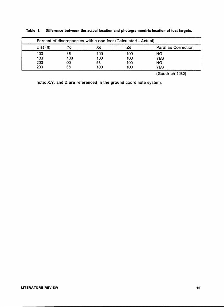
Table 1. Diflerence between the actual location and photogrammetric location of test targets.

Percent of discrepancies within one foot (Calculated - Actual)Dist (ft) Yd Xd Zd Parallax Correction100 65 100 100 NO100 100 100 100 YES200 00 68 100 NO200 68 100 100 YES

(Goodrich 1982)

note: X,Y, and Z are referenced in the ground coordinate system.

LITERATURE REVIEW 10

Ithe average error was still 0.0002 times flying height. "The results indicate that practical

photogrammetry can be done using 35-mm aerial photography and a microcomputer con-

trolled analytical stereo plotter. Although some systematic errors are present in the plotted

values, the magnitudes of the errors are low. These accuracy levels are acceptable for many

photogrammetric purposes." (Roberts and Griswold 1986)

Research studies on acreage calculation from 35-mm photography are extremely limited. The

only publication found analyzed the impact of transmission lines on agriculture production in

the mid-west (Grumstrup et al. 1980). 500 miles (805 km) of seventeen power line segments

were photographed at a nominal scale of 1:1,400. Dot grids were used to compute the acreage

affected by each tower; each dot represented 0.0006 ac. (0.00024 ha). The acreage was ad-

justed if the calculated scale (using the cross arm distance) deviated from the nominal scale.

From this study, Grumstrup found that agricultural practices and the affected acreage varied

with the tower type. Relationships could then be formed between the amount of land withheld

from production and the type of tower. Acreage calculation accuracy was concluded to be

within the desired 10% level, in which three types of errors were found.

• Positive systematic error, up to 3.7%, due to calculating the scale at the top of the trans-

mission tower• Random error of 1.6% due to error in measuring photo distance for calculating the scale• Random error of 6.5% from dot grid estimates

This study Iooked at very small areas on level ground and one must be careful in extrapolating

from these conclusions to larger areas over varying terrain.

LITERATURE REvlEw 11

LOCATION ERROR IN PHOTOGRAPHIC IMAGE

The final section describes the causes and effects of image positional errors on photographs.

By assuming photographs have properties equal to maps, three types of errors are disre-

garded (Spurr 1960, Wood 1949).

• The ground is not perfectly level, thus producing relief errors.• The camera axis is not truly vertical, thus introducing tilt errors.• Camera and photographic material fail to satisfy theoretical requirements completely,

thus giving rise to what may be called instrumental errors.

ln this section, image positional errors will be separated into these three categories, relief, tilt,

and equipment.

RELIEF

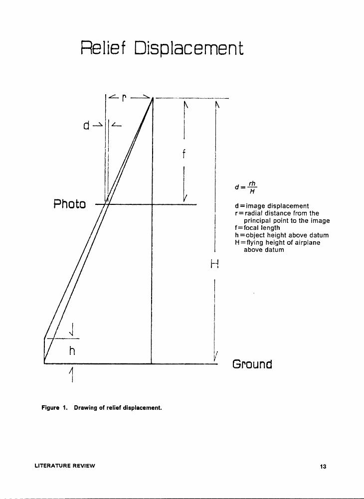
Relief displacement often causes straight roads, fences, and utility lines on rolling ground to

appear crooked on vertical photographs (Wolf 1983). This is especially true near the edge of

a photo with severity dependent on terrain variation. Because displacement causes the tops

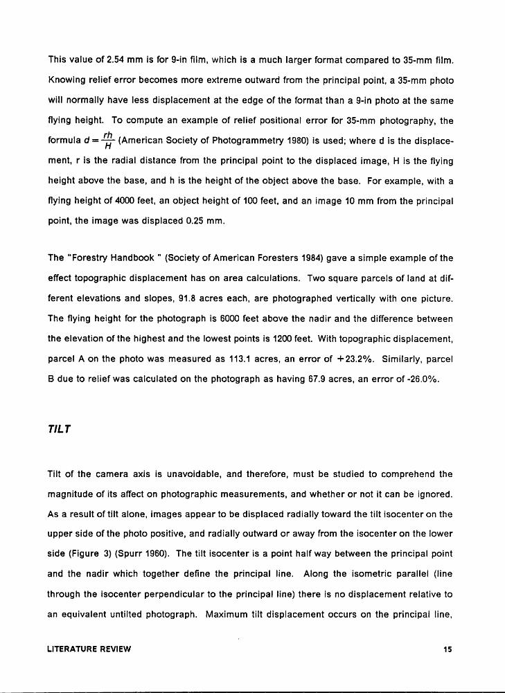
of objects to register further from the principal point than the bottoms (Figure 1), trees appear

to lean outward radially from the nadir, and displacement can cause some features to be ob-

scured from view (Spurr 1960). All objects at the same elevation and equidistant from the

nadir in any direction are displaced equal amounts due to relief (Spurr 1960). Furthermore,

displacement ls inversely related to flying height, and independent of focal length (Spurr 1960).

Relief displacement may be reduced to any deslred amount merely by increasing flying height

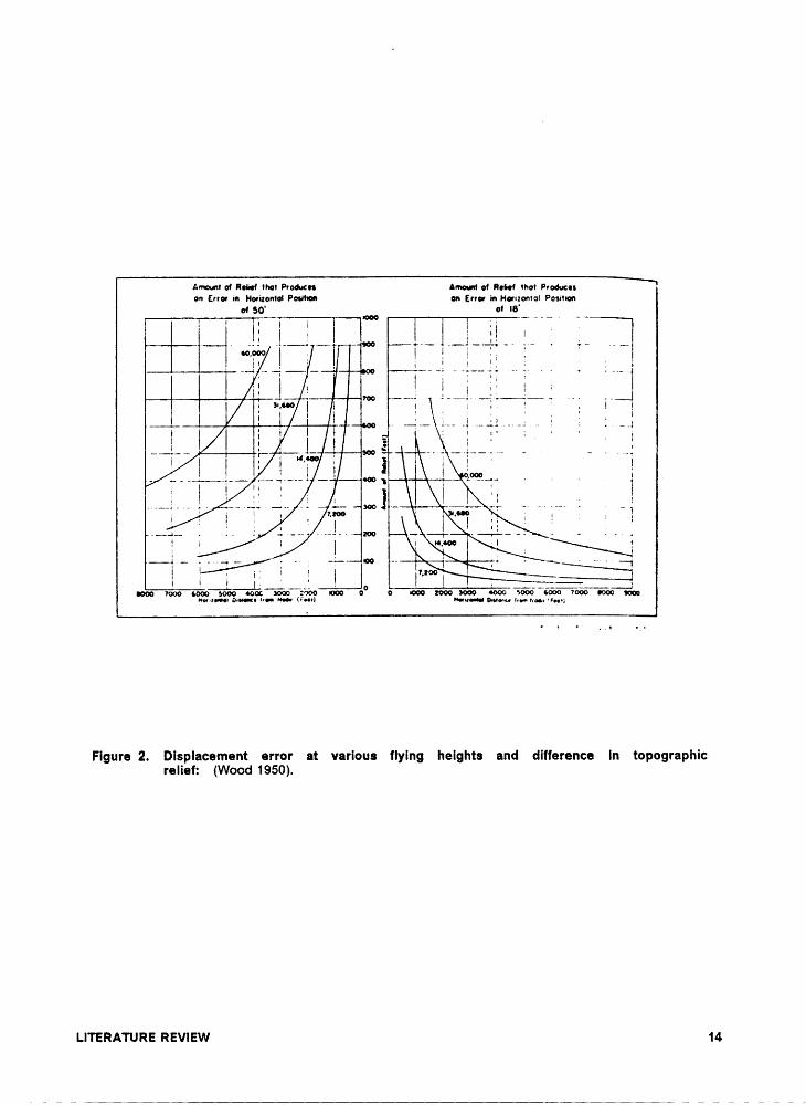
(Figure 2) (Wood 1950). Wood (1949) noted relief errors are frequently 0.10 inch (2.54 mm) or

more.

LITERATURE REVIEW 12

II

4 p...4I

I II I -3I I d- "

I d =image displacement· r=radial distance from the

principal point to the imagef=focal lengthh =object height above datumH=tlying height of airplane

above datum

H

II4 GroundFigure 1. Drawing of relief dlsplacement.

i.ms¤Aru¤6 nzvuaw 13

I

Amoum of Relief mer Producn Amoum of R•6•r mn Produuson Error in Horixonlol Posmorn on Error in Honzomol Posnion

of50' of IB' —1 1 I 1 I°°°·—-T I _1 - -1--1 - ,.,1, - -1-4--. L- . L--

•°·1*°° I ; I I I I Ii i I 11 _1·- 1-- 1 1-4 -4-;- . -. 1r I 1 1 1 II 1 1 II 1 . I I I 1I' _,_- pg ---1 ;---..---....-.;-- .--I

: "·“° I I 1 1 L ·· ? I 1 I I- I I 1 I J

;__ ._ E;1, t fz 1 1 I I . I

.-.._I,..- I I Mi; ß -•I --1I-„-...1- .. . --_:I I é

I 1 I ' I·I *1** =I1I 1 1f 1 6 1 „„} I “= ; 1 1T" °' 55- .••¤ '” 1 1 1 1 ”I

I i I I I II 1 1 ‘ ' 1I”1" 1 II I ’°°T1I ‘1*"*·*· '°° ·· " · 1* · —~ ·—··1—1I E 1 if I 1 I I 11=¤¤ 1 :1I I I 1· I --Ä 1 1, I I · ..1T'.’l."“°--.-.jQN 7000 6000 $000 40K SON 2000 DN 0 0 IGN 2000 SON 4000 5000 GN0 7000 ION WN••e1r•••¤ 0••••¤• Iren N••1r (F•••l

NeuesteFigure2. Displacement error at various flying heights and difference ln topographicreliefz (Wood 1950).

LITERATURE REVIEW 14

This value of 2.54 mm is for 9-in film, which is a much larger format compared to 35-mm film.

Knowing relief error becomes more extreme outward from the principal point, a 35-mm photo

will normally have less displacement at the edge of the format than a 9-in photo at the same

flying height. To compute an example of relief positional error for 35-mm photography, the

formula d =—%— (American Society of Photogrammetry 1_980) is used; where d is the displace-

ment, r is the radial distance from the principal point to the displaced image, H is the flying

height above the base, and h is the height of the object above the base. For example, with a

flying height of 4000 feet, an object height of 100 feet, and an image 10 mm from the principal

point, the image was displaced 0.25 mm.

The "Forestry Handbook '° (Society of American Foresters 1984) gave a simple example ofthe

effect topographic displacement has on area calculations. Two square parcels of land at dif-

ferent elevations and slopes, 91.8 acres each, are photographed vertically with one picture.

The flying height for the photograph is 6000 feet above the nadir and the difference between

the elevation ofthe highest and the lowest points is 1200 feet. With topographic displacement,

parcel A on the photo was measured as 113.1 acres, an error of +23.2%. Similarly, parcel

B due to relief was calculated on the photograph as having 67.9 acres, an error of -26.0%.

TILT

Tilt of the camera axis is unavoidable, and therefore, must be studied to comprehend the

magnitude of its affect on photographic measurements, and whether or not it can be ignored.

As a result of tilt alone, images appear to be displaced radially toward the tilt isocenter on the

upper side of the photo positive, and radially outward or away from the isocenter on the lower

side (Figure 3) (Spurr 1960). The tilt isocenter is a point half way between the principal point

and the nadir which together define the principal line. Along the isometric parallel (line

through the isocenter perpendicular to the principal line) there is no displacement relative to

an equivalent untilted photograph. Maximum tilt displacement occurs on the principal line,

LITERATURE REVIEWU

15

I

lTilt Dnsplacement

d flllI l

2I d=d

=disp|acement due to tllty=principal line distance

from image to isocenterf=focaI lengtht=degrees of tilt

Ground

Figure 3. Drawing of tilt dlsplacement.

Lmsnmuna navisw 16

l

land zero displacement occurs on the isometric parallel (American Society of Photogrammetry

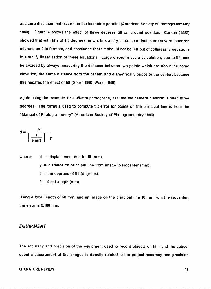
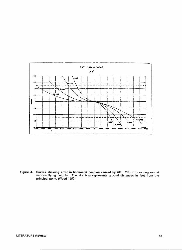
1980). Figure 4 shows the affect of three degrees tilt on ground position. Carson (1985)

showed that with tilts of 1.8 degrees, errors in x and y photo coordinates are several hundredmicrons on 9-in formats, and concluded that tilt should not be left out of collinearity equationsto simplify Iinearization of these equations. Large errors in scale calculation, due to tilt, canbe avoided by always measuring the distance between two points which are about the same

elevation, the same distance from the center, and diametrically opposite the center, because

this negates the effect of tilt (Spurr 1960, Wood 1949).l

Again using the example for a 35-mm photograph, assume the camera platform is tilted threedegrees. The formula used to compute tilt error for points on the principal line is from the

"Manual of Photogrammetry" (American Society of Photogrammetry 1980).

2d =

Sin(I) iI"y

where; d = displacement due to tilt (mm),

y = distance on principal line from image to isocenter (mm),

t = the degrees of tilt (degrees).

f = focal length (mm).

Using a focal length of 50 mm, and an image on the principal line 10 mm from the isocenter,

the error is 0.106 mm.

EQUIPMENT

The accuracy and precision of the equipment used to record objects on film and the subse-

quent measurement of the images is directly related to the project accuracy and precision

LITERATURE REVIEW 17

I

I

TILT DOSPLACEMENTi·3°

Ä; I J llI-I-..J---L„„-J J_.

II<II”°i°°IIIIIIIiIII -20-————*:—····I·—* “~°@°—+ ‘——; I I I :··-+I I I I I I I I IE _ I i-,.·{ I· IIIIIIIIIL I I.

I I IIllllllllälllllllllll·II•···. I =IIIIIIII I"'°° I I’°“°j>§‘

~•O@7§$OxS€¢0@$O@2@§°|0X!°x’Ä()XSXÖÜ€7°(«ÜFigure

4. Curves showing error in horizontal position caused by ti|t: Tilt of three degrees atvarious flying heights. The abscissa represents ground distances in feet from theprincipal point. (Wood 1950)

meRA·ruRe REVIEW 18

outcome. Factors involved In the photogrammetric accuracy include, camera and projector

lens distortions, film fiatness and stability, and precision of the measuring devices. The

equipment can be divided into two operational objectives, initial recording of the light rays,

and the use and measurement of the developed ülm.

Lens quality is very important because all light rays must pass through the assembly. Metric

cameras have calibrated distortion curves, but few tests have been conducted on small formatlenses. Spurr (1960) reported 9-in format camera lens have distortions of 10 micrometers at

the edge. Goodrich (1982), in calibrating a 35-mm camera lens, found the residuals on the

majority of targets measured to be below 20 micrometers, although some points had residuals

in the 40 to 50 micrometer range.

ln recording the images, films have two weaknesses stemming from the fiexibility of the pho-

tographic material. First, film instability, shrinkage and stretching is present in all formats.

However, the 9-in cameras record fiducial marks on the film which allows the instability to be

computationally removed. Second, film flatness, since the material is flexible, the potential

of bowing exists. Large format cameras hold the unexposed film fiat with a vacuum. In both

cases, 35-mm cameras do not have the capacity to correct or control the inherent weaknesses

of the photographic material. Image blur can also be a problem. Excessive movement ofthe

camera relative to the ground is the main cause, and it is therefore necessary to use fast

shutter speeds to eliminate this image-motion (Spurr 1960).

A third shortcoming of 35-mm film is the smaller size ofthe photographs. Enlargement is often

necessary for viewing and is especially necessary for measurement via several alternative

methods. With all the methods though, the image rays must pass through a second lens as-

sembly. Montgomery and Wolf (1986) found that with a tablet digitizer and an overhead pro-

jector, they could achieve measurement accuracies of 5 to 10 micrometers at photo scale.

This system projects small formats, up to 2-inches square. The errors they found included:LITERATURE REVIEW ‘ 19

I

• Tablet digitizer giving incorrect results (found tablet accurate to within .125 mm)• Non-planar film surface• Non-planar digitizer surface• Projector lens distortion• Non-parallelism of projector and digitizer• Decentered cursor reference mark

Montgomery and Wolf (1986) reported surprisingly accurate results, from 5 to 10 micrometers,

and are applying this system for several ongoing close range and terrestrial photogrammetric

research projects, including applications in biostereometrics, traffic movement investigations,

accident reconstruction, and positioning for hydrographic surveys.

SUMMARY

lt follows from the above discussion that topographic relief, tilt displacement, and equipment

inaccuracies greatly affect image positions on photographs, and as such, a study was neces-

sary to find the results of the singular and combined influences of image positional errors in

area estimation. If an image had relief error of 0.25 mm, as computed in the example above,

and tilt error of 0.106 mm in the same direction, and distortion error of 0.04 mm, the one point

would be measured 0.396 mm from its correct location. All the points along a tract boundary

each have independent values of relief displacement, tilt displacement, and lens distortion.

It was theoretically known how and where location of images are changed before conducting

this study, however, the combined effect of the displacements and distortions when calculating

acreages was not known.

LITERATURE REVIEW 20

l

MATERIALS AND METHODS I

It was from this unknown error in area estimation from aerial photographs that this study was

designed. There were two possible experimental designs; actual flights with targets and sur-

veyed ground points to solve for flying parameters such as flying height and camera attitude,

or analytic simulation to control these exterior orientation parameters. Due to the additional

unknowns, lack of factor control, and measurement errors involved in actual experimental

flights, the computational analytic simulation method was used.

Three steps were necessary to accomplish the analytical method. First, an appropriate num-

ber of sample tracts were selected and the boundaries digitized collecting x,y coordinates and

elevations. Second, computer programs converting three dimensional ground coordinates

into two dimensional photo coordinates with the correct adjustments for relief displacement,

camera tilt, and lens distortion were written. Third, for each of the simulations, acreages were

calculated directly from the photo coordinates, and the percent error was computed. From the

percent error data, analyses were made to understand the effects of topographic displace-

ment, tilt, and lens distortion on acreage estimation error.

MATERIALS AND METHODS 21

IDATA COLLECTION

Because of the many combinations ofthe flight parameters to be simulated for each tract, only

four test tracts were used. ldeally, the tracts should sample the range of topographic relief,

tract sizes, and tract shapes. However, by Iimiting the number of sample tracts to four, the

sampled areas were within regions where aerial photographs are often used and where the

results would be most applicable. The Coastal Plain and the Piedmont physiographic regions

both have large intensively managed agriculture and forestry land holdings and hence sam-

pled for this study. Furthermore, the size of the sample tracts was limited to fit entirely on

35-mm film taken with normally used Ienses and at normal flying heights. Actual tract

boundaries were not necessary to complete this study for two simple reasons. First of all, this

study was not undertaken to prove any particular point about a specific piece of land, but to

produce some guidelines on flying height, lens choice, and tilt limitations. Secondly, because

ofthe metes-and—bounds surveying in the East, tracts are irregular and dissimilar.

To acquire the data in the necessary ground coordinates, the four selected tracts were traced

on 7.5 minute USGS topographic maps and digitized. The digitized coordinates were the

intersections of the tract boundaries with the topographic elevation isolines. Two represen-

tative tracts were acquired from the Coastal Plain region and two from the Piedmont region.

The Coastal Plain region is generally level, and was used as it was hypothesized there is little

effect from relief in this area. These two sample tracts were from Murfreesboro, NC and

Franklin, VA topographic maps, and have maximum topographic changes of 48 feet and 19 feet

respectively. Rolling hills dominate the Piedmont area, and this area was chosen for study

because both tilt and relief displacement could be better analyzed. The two sample tracts for

this area were from Crewe West, VA and Keysville, VA topographic maps, and have maximum

elevation differences of 105 feet and 60 feet respectively.

MATERIALS AND METHODSV

22l

I

PHOTOGRAPHIC SIMULATION

To simulate the photographs, ground coordinates were converted to photo coordinates via

collinearity and lens distortion equations. The collinearity equations used seven parameters

and the ground coordinates. Camera attitude (tilt, swing, azimuth), camera exposure station

coordinates (Xl,YI,Zl) and camera focal length (f) were the seven parameters. The collinearity

equations (Wolf 1983) automatically took into account and adjusted the photo image positions

for topographic relief, camera tilt, and focal length.

[Ilz/11(Xg - XI) + M12(Yg — YI) + M13(Zg — Z/)]"’[/Vl21(Xg — XI) + M22(Yg — YI) + /l//23(Zg — ZI)]Y

=where; x,y = photo image coordinates (mm)

f = focal length (mm)

Xg,Yg,Zg = ground coordinates of object (ft)

Xl,Yl,Zl = exposure station coordinates (ft)

M11 = -cos(a)cos(s)¥sin(a)cos(t)sin(s)

M12 = sin(a)cos(s)-cos(a)cos(t)sin(s)

M13 = -sin(t)sin(s)

M21 = cos(a)sin(s)-sin(a)cos(t)cos(s)

M22 = ·sin(a)sin(s)-cos(a)cos(t)cos(s)

M23 = ·sin(t)cos(s)

M31 = -sin(a)sin(t)

M32 = -cos(a)sin(t)

M33 = cos(t)

t = tilt (deg)

s = swing (deg)

MATERIALS AND METHDDS 23

a = azimuth (deg)l

Flying heights of 4,000 feet and 6,000 feet, and lenses of 24 mm and 50 mm lengths were

simulated. These values of tiying heights and lens focal lengths represented commonly used

values. For all of the simulations, the camera was located above the midpoint of a bounding

rectangle which contained the tract, and was not horizontally shified even with tilt of the

camera axis. To implement tilt into the simulation, values of 0, 3, 6, and 12 degrees were

used, with four repetitions of each value by changing the swing and azimuth angles. Tilts less

than three degrees are commonly considered negligible and assumed zero. Tilts of six and

twelve were used as representative values beyond the three degree limit. The four repetitions

within each tilt level had azimuth values of 0, 90, 180, and 270. The respective swing was the

azimuth plus 180 degrees to keep the top of the format oriented north. These four tilt di-

rections, while not covering all possible directions, sampled each tract with a different portion

ofthe tract at the low end of the tilted format. lf the repetitions were all taken from the same

quadrant, the same portion ofthe tract boundary would always be at the low end ofthe ofthe

tilted format. lt is also possible to move the camera exposure station to center the tract with

tilt accounted for, however, this was not done in this study because an error in scale and new

relief errors would be introduced. Lens distortion errors were applied to the computed photo

coordinates for all of the simulations creating results both with and without distortion. The

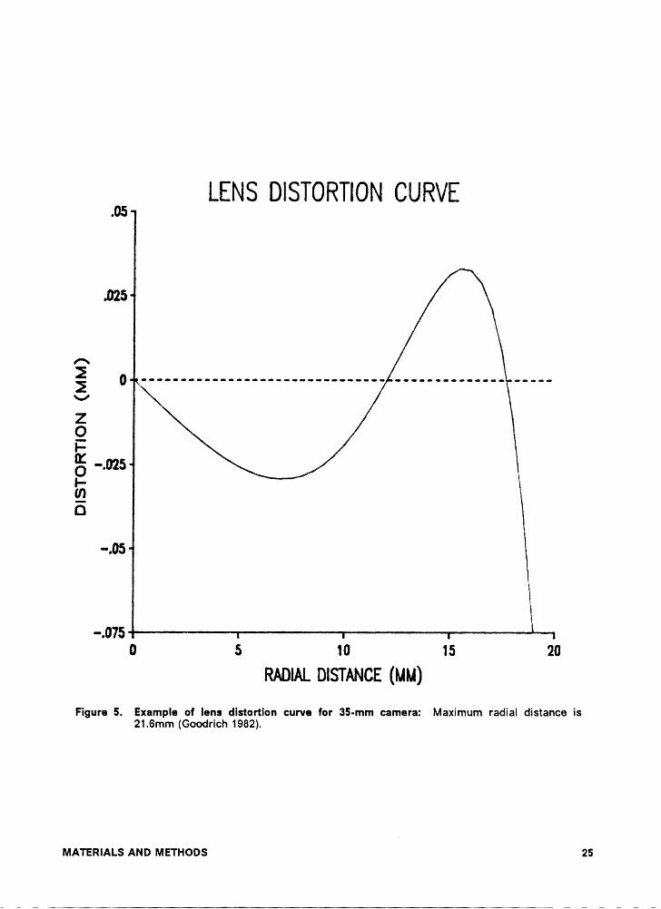
lens distortion curve published by Goodrich (1982) was used to adjust the photo coordinates

in this study. Nineteen sample points were measured on this curve to recreate the specified

model parameters and fitted through least squares regression techniques. The following

equation and Figure 5 were developed through this procedure.

d = -5.96798r + 0.028053r° + 0.00019402r° + ( -7.0935E — 07)r’

where; d = displacement (microns)

r = radial distance to image (mm)

MATERIALS AND METHODS 24

05 LENS DISTORTION CURVE

.025

E2 g ............................... -............- .....\•/

ZOF-'g -.0251-Q0

-.05

L-.075

0 5 10 15 20RADIAL DISTANCE (MM)

Figure 5. Example of lens distortion curve for 35-mm camera: Maximum radial distance is21.6mm (Gocdrich 1982).

MATERIALS Ann msmoos 25

I

Although this displacement curve is not expected to be the same for all 35-mm camera lenses,

it is a known and published example. Since the lens distortion is radial, the photo coordinates

were adjusted using the following two equations.

dx' = x(1 — 7-)

[ dy =y(l — 7)

where; x' and y' = adjusted photo coordinates

x and y = original photo coordinates

d = displacement (mm)

r = radial distance to image (mm)

METHODS OF ANALYSIS

Two values of tract acreage were compared for the analysis. One of which was estimated

from the simulated photographs, and the second was the true ground acres. The true ground

acreage for each tract was calculated directly from the digitized ground coordinates. The

photo acreage estimates, however, were more difficult to define. To begin, the photo area

(mm') was measured directly from the positive or negative transparencies. A conversion

(scale) was then applied to convert the photo units of millimeters to the ground units of feet.

This scale was linear and changed the units without affecting the comparisons. Scale was

calculated by dividing the focal length by the flying height above the terrain elevation. How-

ever, the terrain was not level, and thus, the true scale fluctuates within the format. Therefore,

an average scale (held constant) was used for the conversion, and was calculated by using

the average elevation of the digitized points for each set of flying height and lens focal length

MATERIALS AND METHODS 26

l

lcombinations of each tract. This is a commonly applied procedure during photo interpretation

projects.

Acreage calculation was the primary data needed to reach the goals ofthis project. The photo

coordinates of each tract perimeter were used in the following equation to compute the area

(Brinker and Wolf 1977).

1 HAREA = E- X1 [><,·(y;+« — 16-0]

where; AREA = absolute value

x = x photo coordinate

y = y photo coordinate

i = point number

n = number of points

ifi=1 then i-1 = n

ifi=ntheni+1=1

From the area calculations, percent error was calculated by dividlng the change in acres,

photo estimated minus true, by the true acres and then multiplied by 100.

Visualization of the positional errors was also important for understanding the results and

making recommendations. Actual drawings of the simulated photographs helped in the vi-

sualization. These plots duplicated the simulated photographs with enlargements to easily

discern the errors. Overplotting, for a better comparison, was also available. An example

plot contained one plot without any positional errors, and a second and third plot with dis-

placement intluences of 3, and 6 degrees tilt. This type of analysis showed the general Io-

cation of the positional errors, reproducing what would actually be seen when projecting the

photographs on top of a correct base map.

MATERIALS AND METHODS 27

I

These results of change in acres were best presented in a tabular format. Tabular form fa-

cilitates empirical comparisons and the creation of guidelines from the many available com-

binations of the data. Three example comparisons are explained below, and are only a

sample of the comparisons to be examined. For example, in looking at the two tracts from the

Piedmont region, one observes the impact flying height had on the relief displacement error

as flying height increases from 4,000 feet to 6,000 feet. Secondly, constructed graphs show

specific trends of tilt. lt was unknown how acreage error changed as influenced by tilt, pos-

sibly linearly or exponentially. A graph helped explain and set guidelines for limitations oftilt.

The third example analysis covers the hypothesis that lens dlstortion has minimal influences

on acreage calculation. It was known that lens distortions causes minimal errors of a single

point (0.04 mm), but the summation of these errors was unknown. By comparing different

simulations with and without lens distortlon, an average error due to lens distortion was

computed.

COMPUTER PROGRAMS

For ease of computation and for future applications, computer programs were written to per-

form the steps described above. The four programs, one, digitized the ground coordinates,

two, calculated the true acreage, three, simulated the photographs and calculated the photo

acreage, and four, plotted the desired photographs (Appendixes A, B, C, D). The digitizing

program was written on a Data General Desktop Model 30 using MPBASIC programming

language to interface with a Calcomp 9100 Table Digitizer. The other three programs were

written in Borland Turbo C for use on an IBM PC/AT to run on any IBM compatible personal

computer. The plotting program was written to interface with an HP7475a plotter.

The first program, Mapper (Appendix A), recorded the digitized coordinates and elevations to

an ASCII file. The program first initialized the table to output State Plane Coordinates and the

MATEIRIALS AND METHDDS 28

keyed·in elevations to the nearest foot. Before digitizing, the topographic map was secured I

to the table and the origin was set near the lower left hand corner of the map. The digitlzed

points were the tract boundary corners and the points where the boundaries intersected the

elevation contours. Although there were always small errors in digitizing, these errors were

irrelevant for this study, and the recorded X and Y coordinates became the true coordinates

for acreage calculation and for the photographic simulations. The coordinate file for each tract

was then transferred to an IBM PC/AT file for photographic simulation.

The program Acreage (Appendix B) calculated the control acres from the digitlzed ground

coordinates. These acres were not the true ground acreages, due to digitizing errors. How-

ever, since the same ground coordinates were used in both this program and the simulation

program, this procedure accurately assessed the errors due to photographic properties. This

acreage program utilized the Brinker and Wolf (1977) acreage calculation formula explained

in the methods section. Acreages were recorded to three decimal places, although the com-

puted acres were significant to tive decimal places. More explicitly, as the smallest unit re-

corded during digitization was one foot, an area of one foot square divided by 43560 square

feet per acre is approximately 0.00002 acres.

Photosim (Appendix C) was the main program for this project. Photosim computed the photo

coordinates from the ground coordinates with the given camera orientation and location pa-

rameters. This program utilized the collinearity equations of Wolf (1983). Focal length was

specified in millimeters and flying height was specified in feet. Tilt, swing, and azimuth, in

degrees, controlled the amount and the direction of tilt. By adding 180 degrees to azimuth

when specifying the swing the camera was always oriented north. Exposure station coordi-

nates were in feet, and could have been specified in three ways. The first, and the simplest,

was the center of the bounding rectangle. The program defaulted to these coordinates unless

new coordinates were manually entered, which was the second option. The third option was

available to recenter tracfs on tilted photographs by off-setting the exposure station coordi-

nates appropriately. An eighth parameter, topographic relief factor, allowed flattening out or

MATERIALS AND METHDDSl

29

intensifying the topographic relief. The final step of the program wrote the the input parame-

ters, the resulting photo area (mm'), the scale, and the calculated acres to the screen for each

simulation. Photosim output photo coordinates to a specified file name. An e><tra coordinate

was added to the end of the file which was the location of the tract center on the format.

The final program, Slide (Appendix D), plotted a slmulated photograph on 8.5x11 paper. The

plots could have been overlaid in any combination to show exactly how the photographs ofthe

tracts appeared if enlarged to the same size as a base map. The base map, in this case, was

a photo without positional errors. Since Photosim could also compute photo coordinates

without any positional errors, Slide could plot respective photos with and without errors over

top of each other.

MATERIALS AND METHODS 30

1

RESULTS AND DISCUSSION

To systematically evaluate the results of this project, discussion of the errors will be divided

into three sections: topographic relief error, camera tilt error, and lens distortion error. A

final section will then integrate the results and make several recommendations. This intro-

duction section is necessary to highlight and discuss results pertinent to all three sections.

lt is also important to reiterate that this was a case study with the camera centered over the

tract and with only four tracts used in the simulation. First of all, the error values compared

are the change in acres, photo acres minus the ground acres, divided by the ground acres

then multiplied by one hundred (percent acreage error). As can be seen from Table 2 through

Table 5 the range of the percent acreage error is from -1.723 to 10.233 percent. A negative

value exists if the photo computed acres was less than the true ground acres, and positive if

the photo errors increased the tract size. Secondly, focal length did not change the acreage

errors of relief and tilt when lens distortion error was not included and flying height was held

constant. This fact is very important to aerial photography. At a given flying height, the dis-

tortion of the same images imparted from two different focal length lenses at the same flying

height are proportionately equal, and consequently cancel out when computing acreages.

Thus, the 35-mm format itself did not create or impart more error due to the focal length or the

format size. Finally, at twelve degrees of tilt, the images could not be completely photo-

RESULTS AND DISCUSSION 31

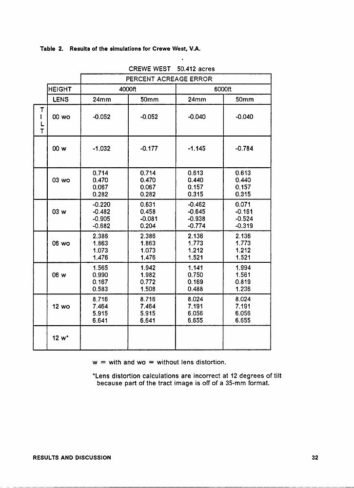
Table 2. Results of the simulations for Crewe West, V.A.‘

CREWE WEST 50.412 acresPERCENT ACREAGE ERROR

HEIGHT 400011 600011L¤~S Eä 591111Tl -0.040 -0.040LT

0.714 0.714 0.613 0.6130.470 0.470 0.440 0.4400.067 0.067 0.157 0.1570.282 0.282 0.315 0.315-0.220 0.631 -0.462 0.071-0.482 0.458 -0.645 -0.161-0.905 -0.081 -0.938 -0.524-0.682 0.204 -0.774 -0.3192.386 2.386 2.136 2.13606 wo 1.863 1.863 1.773 1.7731.073 1.073 1.212 1.2121.476 1.476 1.521 1.5211.565 1.942 1.141 1.99406 w 0.990 1.982 0.750 1.5610.167 0.772 0.169 0.8190.583 1.508 0.488 1.2368.716 8.716 8.024 8.02412 wo 7.464 7.464 7.191 7.1915.915 5.915 6.056 6.0566.641 6.641 6.655 6.655I 11w

= with and wo = without lens distortion.'Lens distortion calculations are incorrect at 12 degrees of tilt

because part of the tract image is off of a 35-mm format.

RESULTS Ann oiscussiou 32

I

Table 3. Results 01 the simulations for Franklin, V.A.

FRANKLIN 29.612 acresPERCENT ACREAGE ERROR

HEIGHT 400011 6000ftLENS 24mm S¤m¤«TI 0.078 0.078 0.051LT

0.797 0.797 0.665 0.6651.185 1.185 0.925 0.9250.209 0.209 0.274 0.274-0.179 -0.179 0.017 0.017-0.209 0.588 -0.439 -0.0340.199 1.091 -0.169 0.301-0.824 -0.176 -0.844 -0.534-1.233 -0.672 -1.114 -0.8682.398 2.398 2.141 2.1413.188 3.188 2.664 2.6641.206 1.206 1.344 1.3440.415 0.415 0.817 1.8171.483 2.445 1.104 1.8742.317 3.411 1.655 2.5600.230 0.959 0.270 0.841-0.604 0.000 -0.280 0.1598.480 8.480 7.879 7.879

12 wo 10.161 10.161 8.996 8.9965.937 5.937 6.180 6.1804.258 4.258 5.062 5.062

w = with and wo = without lens distortion.*Lens distortion calculations are incorrect at 12 degrees of tilt

because part of the tract image is off of a 35-mm format.

RESULTS AND DISCUSSION 33

I

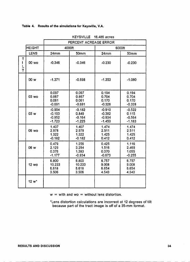
Table 4. Results of the simulations for Keysville, V.A.

KEYSVILLE 16.486 acresPERCENT ACREAGE ERROR

HEIGHT 4000ft 6000ftLENS S¤¤·mTI 00 wo -0.346 -0.230LT

I 00 w -1.371 -0.698 -1.353 -1.0800.097 0.097 0.194 0.1940.867 0.867 0.704 0.7040.061 0.061 0.170 0.170-0.691 -0.691 -0.328 -0.328-0.904 -0.182 -0.910 -0.522-0.103 0.849 -0.382 0.115-0.952 -0.164 -0.934 -0.564-1.723 -1.225 -1.450 -1.1831.407 1.407 1.474 1.474

06 wo 2.978 2.978 2.511 2.5111.322 1.322 1.425 1.425-0.182 -0.182 0.412 0.4120.479 1.256 0.425 1.1162.129 3.294 1.516 2.4690.376 1.383 0.370 1.055-1.177 -0.934 -0.673 -0.2556.800 6.800 6.757 6.757

12 wo 10.233 10.233 9.008 9.0086.618 6.618 6.654 6.6543.506 3.506 4.543 4.543I E N 1111w = with and wo = without lens distortion.'Lens distortion calculations are incorrect at 12 degrees oftilt

because part of the tract image is off of a 35-mm format.

REsuLTs AND DISCUSSION 34

1

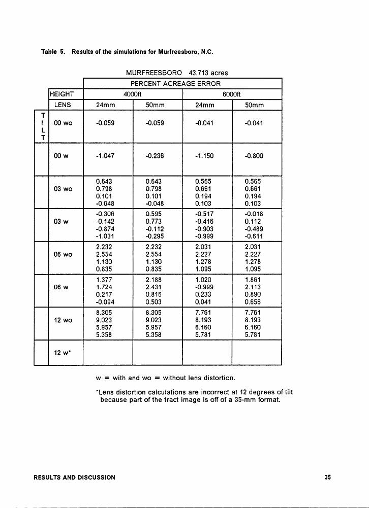
Table 5. Results of the simulations for Murfreesboro, N.C.

MURFREESBORO 43.713 acresPERCENT ACREAGE ERROR

HEIGHT 4000Ft 6000ftLE~STl 00 wo -0.041LT

0.643 0.643 0.565 0.5650.798 0.798 0.661 0.6610.101 0.101 0.194 0.194-0.048 -0.048 0.103 0.103-0.306 0.595 -0.517 -0.018

03 w -0.142 0.773 -0.416 0.112-0.874 -0.112 -0.903 -0.489-1.031 -0.295 -0.999 -0.6112.232 2.232 2.031 2.0312.554 2.554 2.227 2.2271.130 1.130 1.278 1.2780.835 0.835 1.0951.0951.3772.188 1.020 1.8611.724 2.431 -0.999 2.1130.217 0.816 0.233 0.890-0.094 0.503 0.041 0.6568.305 8.305 7.761 7.761

12 wo 9.023 9.023 8.193 8.1935.957 5.957 6.160 6.1605.358 5.358 5.781 5.781I 12 1 1111w = with and wo = without lens distortion."Lens distorlion calculations are incorrect at 12 degrees of tilt

because part of the tract image is off of a 35-mm format.

Rssuurs AND mscussiou 35

graphed on the 35-mm format. Thus, the percent error for simulatlons with lens distortion atI

twelve degrees of tilt were invalid because the tracts could not be photographed completely.

Because the lens distortion Is undefined for points off the format, these acreages were not

used at anytime in the discussion. The results of twelve degrees tilt without lens distortion,

however, were used, as the size of the imaging plane is ultimately irrelevant.

RELIEF

Knowledge of relief displacement magnitude alone is the first building block necessary to ex-

amine the effects of the three photo-caused positional errors on area estimates. As camera

tilt and lens distortion are added, relief displacement error becomes compounded with them.

For this reason, only untilted simulatlons without lens distortions will be analyzed in this sec-

tion.

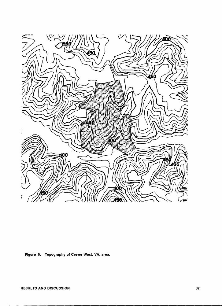
The ranges of topography sampled exemplifies what is typically found in the Piedmont

(Figure 6 and Figure 7) and in the Coastal Plain areas of the southeast (Figure 8 and

Figure 9). As was expected, little error was caused by topographic reliefdisplacement in area

estimation (Table 6), although a more consistent difference between the Piedmont and

Coastal Plain tracts was hypothesized. The average error was -0.167 and +0.007 for the

Piedmont and coastal plain tracts, respectively. The range of the results was from -0.346 to

+0.078, with the two Piedmont tracts having the lowest and the highest errors in absolute

terms. Thus, tract boundary location in relation to the topography had more impact on the

error than the maximum range of topographic variation. That is, the tract boundaries In the

Piedmont have opportunity for greater relief displacement of a specific point, but there was a

compensating Interaction of these point displacements. Moreover, the Piedmont areas with

the greater relief, did not conclusively produce the worst absolute error. In fact, the tract with

the largest relief variation, Crewe West with 105 feet, had the lowest errors, -0.052 and -0.040,

RESULTS AND DISCUSSION4

36

4-** } ’ ‘Q

J O

e7·ä=[[[%;£ „

/ vr?

if „ 7 j; · Q =5 1.,;.2 gib E \/"Ü'Ä[a‘L;1/[igQMP \\ j 1

E«¢’Ü7?’il‘> »

· ,;le’.·:»;<¢',·· 44'” _, 4’ ’ ‘ 7 \,,a 7 w M [ [· N' /7 1, y 4/\ 7 Q. 1· /; [

...Flgure6. Topography of Crewe West, VA. area.

Rssuus AND mscussucu 37

°’B1=e.._[ ___

af rf;

6 Ä ÄÜÄJFFF

Figure 7. Topography of Keysville, VA. area.

40Q

C

A,42

4 4Ä 2~’ J4, 7, 4IW

·’ 4

Figure 8. Topcgraphy of Murfreesboro, N.C. area.

Rssuus Ann ouscussiou ss

I

I

Ä·‘5

·A

,_xß”Q’

·’ ’ ,’ ,, ß

X EFI)Ä (L xx. \ I

Figure 9. Topography of Franklin, VA. area.

RESULTS AND DISCUSSION 40

1

I

ITable 6. Percent acreage error from rellef displacement.

PERCENT ACREAGE ERRORPIEDMONT COASTAL PLAIN

TRACT CREWE. KEYS. MURF. FRANK.MAx. RELIEF 105 rr ß 48 ft 19 rr

FLYING HEIGHT4000 fl 0.078

FLYING HEIGHT6000 fl -0.040 -0.230 -0.041

AVERAGE -0.167 0.007

RESULTS AND DISCUSSION 41

l

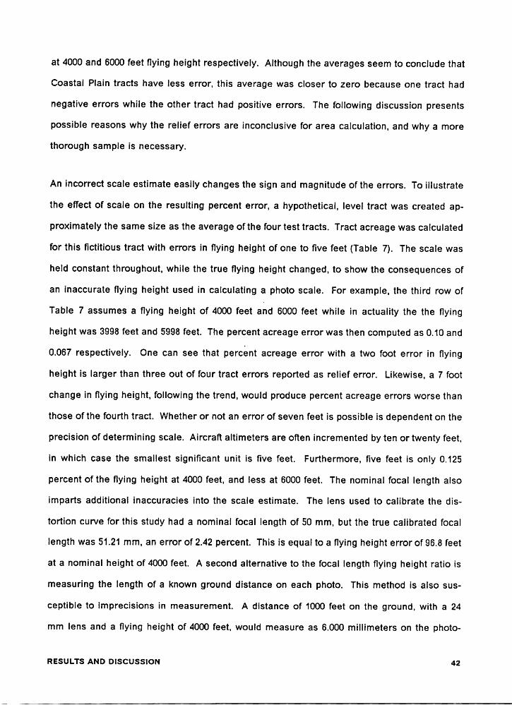
lat 4000 and 6000 feet flying height respectively. Although the averages seem to conclude that

l

Coastal Plain tracts have less error, this average was closer to zero because one tract had

negative errors while the other tract had positive errors. The following discussion presents

possible reasons why the relief errors are inconclusive for area calculation, and why a more

thorough sample is necessary.

An incorrect scale estimate easily changes the sign and magnitude of the errors. To illustratethe effect of scale on the resulting percent error, a hypothetical, level tract was created ap-

proximately the same size as the average ofthe four test tracts. Tract acreage was calculated

for this flctitious tract with errors in flying height of one to flve feet (Table 7). The scale was

held constant throughout, while the true flying height changed, to show the consequences of

an inaccurate flying height used in calculating a photo scale. For example, the third row of

Table 7 assumes a flying height of 4000 feet and 6000 feet while in actuality the the flying

height was 3998 feet and 5998 feet. The percent acreage error was then computed as 0.10 and

0.067 respectively. One can see that percent acreage error with a two foot error in flying

height is larger than three out of four tract errors reported as relief error. Likewise, a 7 foot

change in flying height, following the trend, would produce percent acreage errors worse than

those of the fourth tract. Whether or not an error of seven feet is possible is dependent on the

precision of determining scale. Aircraft altimeters are often incremented by ten or twenty feet,

in which case the smallest signiflcant unit is tlve feet. Furthermore, five feet is only 0.125

percent of the flying height at 4000 feet, and less at 6000 feet. The nominal focal length also

imparts additional inaccuracies into the scale estimate. The lens used to calibrate the dis-

tortion curve for this study had a nominal focal length of 50 mm, but the true calibrated focallength was 51.21 mm, an error of 2.42 percent. This is equal to a flying height error of 96.8 feet

at a nominal height of 4000 feet. A second alternative to the focal length flying height ratio is

measuring the length of a known ground distance on each photo. This method is also sus-

ceptible to imprecisions in measurement. A distance of 1000 feet on the ground, with a 24

mm lens and a flying height of 4000 feet, would measure as 6.000 mlllimeters on the photo-

REsul:rs AND DISCUSSION 42

I

Table 7. Effect flying height error has on percent acreage error, 4000ft and 6000ft are used Incalculating respective tract acres.

PERCENT ACREAGE ERROR FOR CHANGE IN ACTUAL FLYING HEIGHTASSUMED HEIGHT 4000 ft I ASSUMED HEIGHT 6000 ftFLYING COMPUTED PERCENT FLYING CONIPUTED PERCENTHEIGHT ACRES ERROR HEIGHT ACRES ERROR

4000ft 0.000 I 6000It 35.000 0.0003999“ WÄI5999“3998ft0.100 I 5998ft 35.023 0.0673997“ äßl 5997“ äß3996fl 35.070 5996lt 35.047 0.133

t d _t actual height 2compu e acres — rue acres >< assumed height

RESULTS AND DISCUSSION 43

graph. With a flying height of 3995 feet, this same ground distance would measure as 6.0075l

mm. The equipment commonly used to measure Iengths on photographs is not accurate to

seven micrometers.

For level tracts, the value of the flying height above the terrain is easily derived as the flying

height above mean sea level, or some other datum, minus the elevation of the terrain above

this datum. For tracts with terrain variation however, the scale of the highest point is larger

than the scale of the lowest point. This variation in scale is the actual affect of relief. Points

of higher elevation have a larger scale and are thus imaged further from the principal point.

This discussion is to point out that selection of one scale for a tract or the whole format is

difficult. lf one uses the flying height above the highest tract elevation to compute scale, the

estimated acreage would be too low. Likewise, if the lowest elevation was used to compute

the scale, the tract acreage would be positively biased. The difference between the Piedmont

and the Coastal Plain average errors could possibly be from a difference in computing the

elevation in which the aircralt is 4000 or 6000 feet above.

In the scale calculation for this study, the specified flying height was defined as the height

above the average terrain elevation. The average terrain elevation was further deüned as the

simple average of the digitized points. ln the case of the Franklin tract, a disproportionate

number of points were digitized at the lower elevations than the higher elevations. When, in

fact, the majority of the tract was a plateau at the higher elevation. This caused the actual

flying height to be slightly lower than the nominal height over a majority of the tract thereby

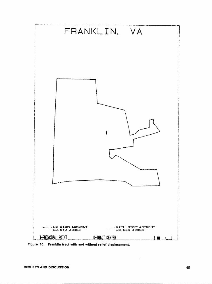
increasing the true scale in these areas. By plotting the simulated photographs with and

without relief error at 4000 feet using a 50 mm lens, one can see that the actual error is very

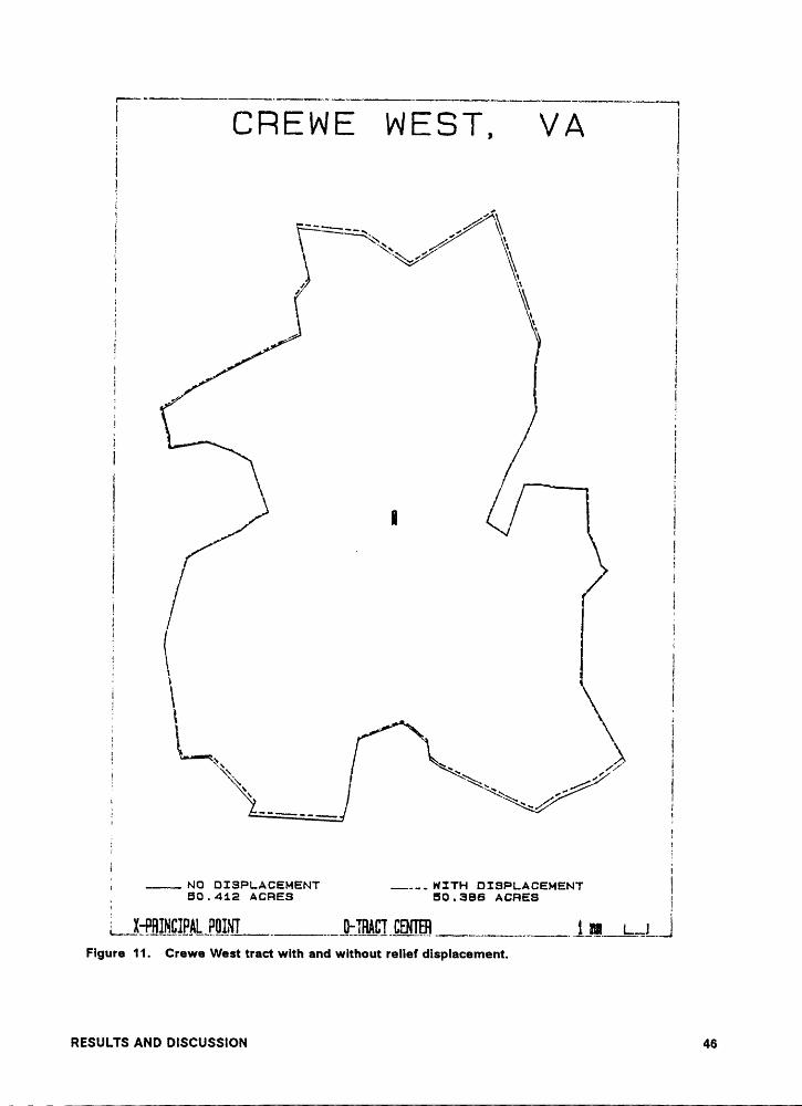
small (Figure 10). Likewise, Figure 11 through Figure 13 show the displacement errors for

the other three tracts. Notice for the Crewe West tract, the displacement error, although large,

was compensating. Part of the tract was displaced outward, while an equal section was dis-

placed inward.

RESULTS AND DISCUSSION 44

I

-„..........._................_..,........—_,,,.....,_,_,____I II F FI A N K I. I N, V A II

I II I

I II{I II II II III ._ II ‘¤

I’ II“II ' II II III [Ä IIIII

.....-——----——·——·-—-——-. II " \ II I; II II II II III II

.......„.. NO DISPLACEMENT .....-- WITHDISPLACEMENTI28 • 812 ACREB 29 . 635 ACREB IL...I:EIIlI@EIIi...I‘.IIlI{I..--....II·lMH.I!.EI{[.EB..„-...--„--...i.l!...;..I...I

Figure 10. Franklin tract with and without relief dlsplacement.

nssuus Ann mscussnou 45

1Q

1 C F? E W E W E S T, V A TQ1

Q QQ Q

#’ Q1 ~-.___ / 11 1V \ 1Q 1 Q1 Q1 J

QS / Q QQÄQ Q_/?

1Q 1Q QQ 11 Q Q(

Q Q1 ’ QQ 1Q1 QQ 1Q Q gQ \1 QQ 2 1Q Q

1 \ \„_ /’

P ‘··———————- 1' Q11

1; ...... NO DISPLACEMENT ....-- WITH QQ 60.412 Acnas 60.666 Acnas QL„l:P.HlQi£lEAL..E&lN.l...-...„--„.Q:lMZI ._..„„...._„.--._.... .i._m.„._;..„L.Q

Figure 11. Crewe West tract with and without relief displacement.

RESULTS AND DISCUSSION 46

II

II———·————·—···—·—·—·····—·—··——·—·—·———~·———·——···—·-··~———·

I I< E Y S V I I. I. E , VAIIIIIII

I IÜ

IIII \ IIIIn

II \$ II II II IA II II III ....... NO DISPLACEMENT .......... WITH DISPLACEMENT

I 18 . 488 ACRE8 18 . 429 ACRE8 IFigure 12. Keysville tract with and without rellef displacement.

RESULTS AND DISCUSSION 47

I

I MUFIFFIEESBORO, NC I

IIIII &/ü II 1I · I

I II II II II II

LII II I

II NO DISPLACEMENT WITHDISPLACEMENTI43 . 731 ACFIES 43 . 705

ACFIESFigure13. Murfreesboro tract with and without relief displacement.

RESULTS AND DISCUSSION 48

lNo deflnite conclusions can therefore be drawn regarding whether or not the Piedmont has

more or less relief error than the Coastal Plain, when caiculating acreages because there are

other factors involved. First of all, the compensating or additive influences of relief displace-

ment is different for centered tracts than for off-center tracts. These off-center tracts were not

simulated in this study, and the relief effects are unknown. Furthermore, from the discussion

on scale, it is apparent that the imprecislon of scale can overshadow relief error for either

region. The variance, on the other hand, was obviously greater for the Piedmont region. This

was supported by the fact that the two Piedmont tracts had the largest and the smallest ab-

solute errors. Also, the variance of the movement of each point on the tract boundary was

larger for the Piedmont than the Coastal Plain because of the greater terrain relief. The im-

portant observation here is the magnitude of the error. As will be brought out in the camera

tilt and lens distortion sections, relief displacement was small in relation to the other posi-

tional errors.

The second important aspect of the investigation of relief displacement was observing the

impact of flying height. By subtracting t_he absolute value of the percent error of the 4000 feet

flying height simulation from the percent error of the 6000 feet flying height simulation, the

magnitude of change due to relief errors for a change in flying height was computed. As was

expected, an increase in flying height decreased the error due to topographic variation in all

cases (Table 8). The average absolute error at 4000 feet was 0.134, while for a flying height

of 6000 feet the error was 0.091 for the four tracts. Thus, the average improvement in the

percent acreage error was 0.043. The results also show that in these four example tracts, the

tract with the largest error improved the most when flying height was increased. Since the

focal length of the lens had no effect on the relief error, selection of flying height could be in-

creased to reduce topographic relief error to any desired level, and the focal length increased

to retain a simular scale.

RESULTS AND DISCUSSIDN 49

I

I

Table 8. Improvement of percent error from relief dlsplacement by increasing flying height.

PERCENT ACREAGE ERRORPIEDMONT COASTAL PLAIN

TRACT CREWE. KEYS. MURF. FRANK. AVG|%e| *RELIEF 105 rx 48 rx 19 n 58 n1@¤0 6ÄÄÄ6000

ft -0.040 -0.230 -0.041 0.051 0.091

IMPROVE- 0.012 0.116 0.018 0.027 0.043MENT

' AVG|%e| is the average of the absolute value of the four tracts.

RESULTS AND DISCUSSIONU

50

l

CAMERA TILT

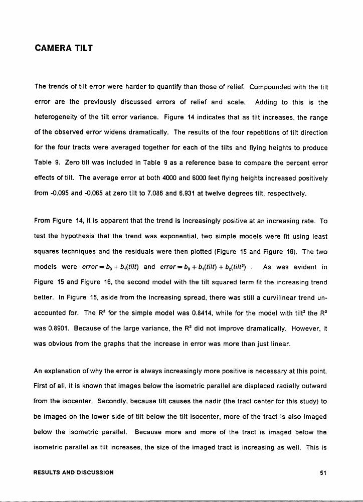
The trends of tilt error were harder to quantify than those of relief. Compounded with the tilt

error are the previously discussed errors of relief and scale. Adding to this is the

heterogeneity of the tilt error variance. Figure 14 indicates that as tilt increases, the range

of the observed error widens dramatically. The results of the four repetitions of tilt direction

for the four tracts were averaged together for each of the tilts and flying heights to produce

Table 9. Zero tilt was included in Table 9 as a reference base to compare the percent error

effects of tilt. The average error at both 4000 and 6000 feet flying heights increased positively

from -0.095 and -0.065 at zero tilt to 7.086 and 6.931 at twelve degrees tilt, respectively.

From Figure 14, it is apparent that the trend is increasingly positive at an increasing rate. To

test the hypothesis that the trend was exponential, two simple models were flt using least

squares techniques and the residuals were then plotted (Figure 15 and Figure 16). The two

models were error= b„ + b,(tilt) and error= bo + b,(tiIt) + b2(filt2) . As was evident in

Figure 15 and Figure 16, the second model with the tilt squared term fit the increasing trend

better. In Figure 15, aside from the increasing spread, there was still a curvilinear trend un-

accounted for. The R2 for the simple model was 0.8414, while for the model with tilt2 the R2

was 0.8901. Because of the large variance, the R2 did not improve dramatically. However, it

was obvious from the graphs that the increase in error was more than just linear.

An explanation of why the error is always increasingly more positive is necessary at this point.

First of all, it is known that images below the isometric parallel are displaced radially outward

from the isocenter. Secondly, because tilt causes the nadir (the tract center for this study) to

be imaged on the lower side of tilt below the tilt isocenter, more of the tract is also imaged

below the isometric parallel. Because more and more of the tract is imaged below the

isometric parallel as tilt increases, the size of the imaged tract is increasing as well. This isRESULTS AND DISCUSSION 51

I

15

10 ¤

ut

0 ä5li BM ¤UIIld

‘*U3*····························

-50 3 6 9 12

DEGREES TlLT

Flgure 14. Scatter plot ol percent acreage error and degrees of tilt

nssuurs Ann mscussnou sz

II

Table 9. Result of slmulatlons for lncreasing tllt and all four tracts averaged together.

PERCENT ACREAGE ERRORTILT DEG. HEIGHT FT. MIN MAX AVERAGE VARIANCE

ÄÄ

¤4000 -0.182 3.188 1.643 0.865

¤6000 0.412 1.629 0.386*2 *222 Äß Ä

12 6000 9.008 6.931 1.711

RESULTS AND DISCUSSION 53

I

4 RESIDUALS FOR TI LT ERROR PREDICTIONI ä

E D2 { U

B { Ü

IJ o ----------L-E--------Q I EU) •III : Q U: ¤ U

·2 : Cl Qv EJ{ ¤I Cl

..4 I

-2 0 2 4 6 8PREDICTED PERCENT ERROR

Figure 15. Plot ol resldual and predlcted values ol percent error for model error=b,,+b,(tiIt).

RESULTS AND mscusslou 54

{4 RESIDUALS FOR TILT ERROR PREOICTION

I 6

2 { ¤I ¤ E: “ ä6 ¥° E ¤3 „ .........ä....................................Fl .....E = E E0:{

El{ _2

:U Q

{ ¤: Ü

: El

-4-2 0 2 4 6 6PREDICTED PERCENT ERROR

Figure 16. Plot ol residual and predicted values of percent error for modelerror= b,+ b,(tIIt) + b,(tilt’).

{ RESULTS AND DISCUSSION 55

apparent when investigating the trends of the three tilt simulations. How off-center tracts

compare area-wise is unknown from this study.

Furthermore, a pattern of the percent error existed within the four repetition of each tilt de-

pendent on the tract shape. As the tilt direction rotated from north, to east, to south, and to

west, relations between the tract shape and tilt direction were formed. When the camera was

oriented in such a way that a long narrow section of the tract was in the lower half (downhill

portion) of the tilted format, the area estimate was less than ifthe narrow section was located

in the upper half (uphill portion) of the frame. Keysville has a long section in the south-east

corner and is an example of this relationship. The percent error at six degrees tilt and 4000

feet flying height was -0.182 when the tilt was directed westward (uphill portion of the tilt to-

ward the west), and 2.978 tilted eastward (uphill toward the east). Similarly, if the bulk of the

tract was in the downhill portion of the format, the area estimate was greater than if the bulk

was located in the uphill half of the frame. The Franklin tract is an example of this when the

camera is tilted toward the east. Therefore, tilt error was related to the direction of tilt inter-acting with the shape of the tract. This is an example of where the limited number of tracts

of a case study limits the inferences of the results. More tracts of different shapes are nec-

essary to verify the tilt errors.

The question then arises whether or not flying height had an additional impact on the tilt error.

The difference between the average error for 4000 feet and 6000 feet at the three tilts was

0.018% at three degrees, -0.014% at six degrees, and -0.155% at twelve degrees. The maxi-

mum difference between 4000 feet and 6000 feet elevation at any tilt was -0.155% error.

However, the higher altitude error was not consistently better. At three degrees of tilt, the

error at 6000 feet was larger than the error at 4000 feet by 0.018 percent. More simulations

are necessary before one can conclude that 6000 feet has consistently lower or higher tilt er-

ror than 4000 feet. From these results, a change in flying height did not appearto change the

acreage error due to tilt.

'

RESULTS AND Dlscussl0N 56

IA second part of tilt error, as flying height increases, was the variance of the error at a given

tilt. As mentioned earlier, the variance of the error increased as tilt increases, However, the

data suggest that the variance was lower at higher altitudes when stratifying the error by flying,

heights (Table 9). By increasing the flying height from 4000 feet to 6000 feet, the variance

dropped more than half for all degrees of tilt tested. This was also evident by comparing the

range of the percent errors. The columns labeled MIN and MAX contain the observed mini-

mum and maximum errors for each tilt•height combination. The decrease in variance at

higher altitudes could be the compounding effect of relief displacement. With an increase in

altitude the topographic displacement decreased. The ratio -:7 in the displacement equation

was lower for the higher altitude and thus the images were displaced less causing the effect

to be less in tilted photographs. This still holds true for tilted photographs, and therefore with

the 6000 feet height, the topography contributed less to the compounded error. One could also

hypothesize that the improvement was due to a change in scale. As scale decreases, the

points were imaged closer to the isometric parallel and displaced less due to tilt. Thus, the

tilt error and variance would decrease. Following from this conclusion, a shorter focal length

lens would also have the same effect on the variance. However, focal length did not change

the acreage error. Consequently, changing the scale, by using a shorter focal length lens, did

not change the variance.

LENS DISTORTION

From the above discussion, it was noted that a change in the focal length had no effect on the

relief acreage error, or the tilt acreage error at a given flying height. The focal length, there-

fore, can be used to appropriately match the photographic scale at any flying height to the

project without increasing or decreasing the error. This, however, was true only without lens

distortion. By adding lens distortion, the derived errors were compounded with tilt, topogra-

phy, flying height, and focal length. The distortion affect is radial, causing the imaged point

RESULTS AND DISCUSSIONl

57

l

to be displaced inward or outward relative to the principal point. All summaries and conclu- 1

sions of lens distortion effects are for this distortion curve only.

Overall, with lens distortion, the computed tract acres were reduced 0.686 percent

(Table 10). This was calculated by subtracting the percent error without distortion from the

percent error with distortion for each of the tracts. Negative values indicated the lens dis-

tortion caused a reduction of the imaged tract size. The results of twelve degrees tilt were

withheld from the computations for Table 10 because the results with lens distortion ofthis tilt

were invalid. Because tilt errors were mostly positive, lens distortion improved the area es-

timates for these tracts. However, for the photographs with zero tilt, lens distortion made all

the area estimates less than the true acreage.

Image distortion is dependent on where the image’s bundle of light rays pass through the lens,

consequently scale most directly dictates the path of the rays. The other influencing factors

were tilt and topography. Assuming tracts are fairly regularly shaped, that is, they are not

convoluted, the points on the tract boundary have nearly the same radii from the tract center.

Following this assumption, one could adjust the scale so that a majority of the tract boundary

lines are imaged through the lowest distortion circumference of the lens. As one can see in

Table 10, the lowest error was at 4000 feet with a 50 millimeter lens. This was because the

image rays of the tract boundaries passed through the outer section of the lens where dis-

tortion was low. lf error, and possibly biases, of -0.686 are too high, each lens should be cal-ibrated. Then, depending on the size of the tract, flying height and lens focal length can be

matched to allow a majority ofthe important light rays to pass through the low distortion area.

The results of this procedure could possibly reduce the error from the worst average error of

-1.073 percent for this lens, to the best average error of -0.183 percent. Again, these results

are for centered tracts, radial lens distortion will affect off·center tracts in a different way.

To understand why the overall average was -0.686 for this lens, example errors were com-

puted for a circle. A circle is the worst case because all points are displaced an equal positive

RESULTS AND DISCUSSION 58

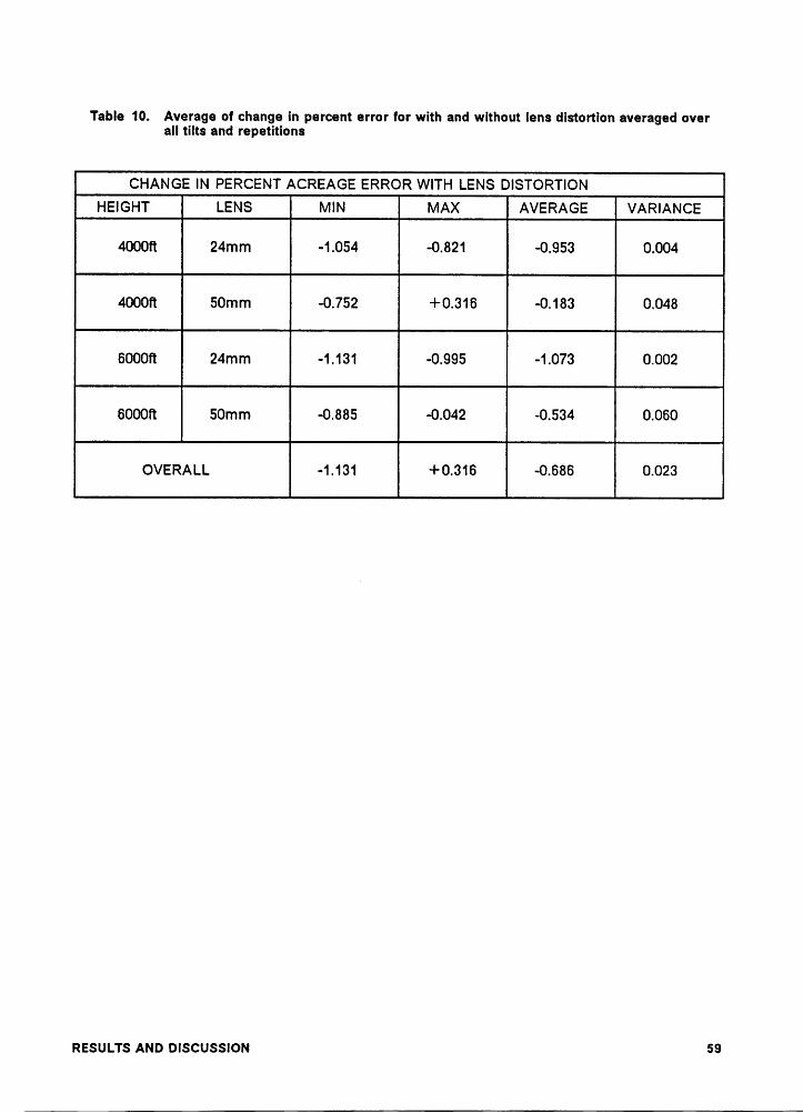
Table 10. Average of change ln percent error for with and without lens dlstortlon averaged overall tilts and repetitlons

CHANGE IN PERCENT ACREAGE ERROR WITH LENS DISTORTIONHEIGHT LENS ß MAX AVERAGE vARuANca

4000ft -0.752 +0.316 -0.183 0.048

OVERALL -1.131 +0.316 -0.686 0.023

RESULTS AND DISCUSSION 59

I

Ior negative amount. Figure 17 shows the percentage error for circles of radius 0.0 to 20

millimeters. Twelve millimeters is the largest circle completely imaged on the 35-mm format.

From this curve, which is valid for this lens distortion curve only, one can see the range of

error was -1.3 to +0.5. Also noticeable is the fact that a majority ofthe curve was negative.

This supports the results of -0.688 change in percent error due to lens distortion.

Tilt also had a slight impact on the lens distortion error. By tilting the camera, the images of

a circle are no longer equidistant from the principal point, and thus all images are not dis-

torted identically. Table 11 shows this was true for the sample tracts also. As tilt increases,

lens distortion has less ofa compounding affect on the estimates. For the vertical simulations,

the difference in percent error with and without distortion was -0.807. At six degrees of tilt the

change in error was -0.803 for the average over all scales. Thus, lens distortion errors were

maximum on vertical photographs and improved slightly as tilt increases.

REsULTs AND Discussion 60

SLENS DISTORTION PERCENT AREAL ERROR”\// \0

1“‘ -.6E / 1[L

1-1 Ag

1-1.5

0 5 10 15 201:112011-; RA¤1us (um)

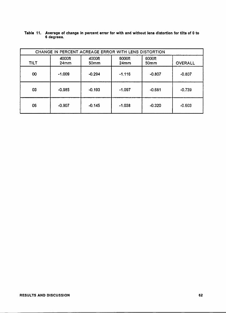
Table 11. Average ol change in percent error for with and without lens distortion for tilts of 0 to6 degrees.

CHANGE IN PERCENT ACREAGE ERROR WITH LENS DISTORTION4000fI 4000ft 6000ft 6000ft

TILT 24mm 50mm 24mm 50mm OVERALL

RESULTS AND DISCUSSION 62

SUMMARY AND CONCLUSION

Three major contributors in the positional errors have been discussed and analyzed. The

worst error achieved was slightly over ten percent, and the best was zero percent error.

Separating the acreage error into its component parts, relief averaged -0.080 percent error,

camera tilt averaged +2.227 percent error, and lens distortion averaged -0.686 percent error.

The overall average error incorporating all factors was 0.363%. This average included all

simulations from zero to six degrees of tilt. The e><tent to which these results affect the use

of aerial photography to compute areas is a function of how well the actual applications imi-

tate the simulations performed in this study. Mainly, all simulations in this study had the ex-

posure station directly over the midpoint of the tract’s bounding rectangle. Given this

situation, many of the image positional errors are compensating when computing areas.

Figure 18 shows the correct Keysville tract without any positional errors overlain with a sim-

ulated photograph. The simulated photograph has a tilt of six degrees, flying height of 4000

feet and a 50 mm lens with distortion. At this scale the error is visible, and the actual differ-

ence in acres is 0.543, 3.294 percent of the 16.486 true acres.

Topographic relief has the potential to create large errors. However, the realization of this

potential was dependent on the tract boundary location relative to the topography. Crewe

West, with 105 feet elevation difference between the highest and the lowest points, had a lower

SUMMARY AND c0NcLUsl0N 63

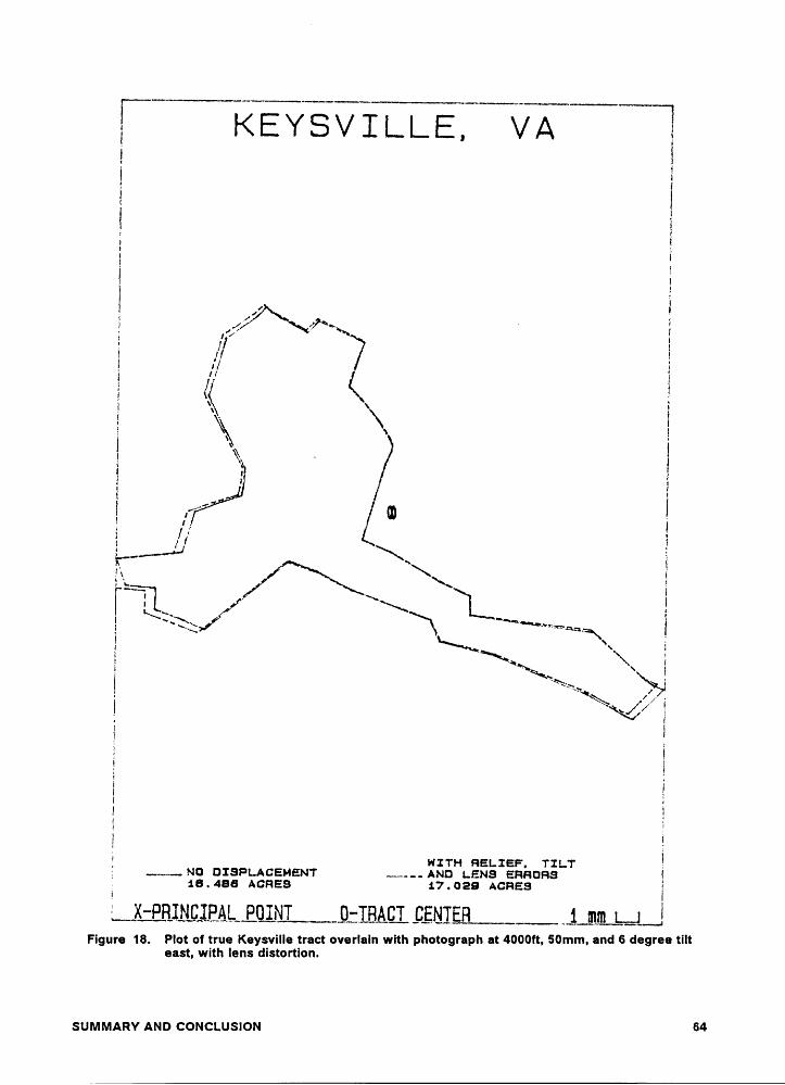
1 K E Y S V I L L E, V A 1·

11 1F 11 1

11 111g}°·~„„~\.F

/ 11:111 11 \\ \\ 1

1 \ · 11 1 ·1 1- I1

kx 1§ „ ———_—-le Ä

\ .

1 11 ~«„„ 111

11 111 11 Z1 11 11 1WITH FIELIEF, TILT......„.... ND DISPLACEMENT .....-..- AND LENS ERFIDFIS 1

i 16 . 466 ACRES 17 . 029ACFIESL„Ä(;EB„I.1§1.Ü„I.E1Ä.1„..P.(ÄlJ1L1._-1];IBA@lQENIEH _ .-..„-L1.F1FmFigure18. Plot of true Keysville tract overlain with photograph at 4000ft, 50mm, and 6 degree tilt

east, with lens distortion.

'

SUMMARY AND CONCLUSION 64

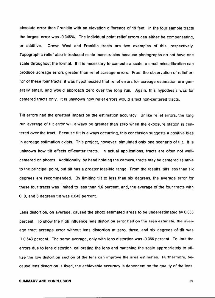
labsolute error than Franklin with an elevation difference of 19 feet. ln the four sample tracts

the largest error was -0.346%. The individual point relief errors can either be compensating,

or additive. Crewe West and Franklin tracts are two examples of this, respectively.

Topographic relief also introduced scale inaccuracies because photographs do not have one

scale throughout the format. lf it is necessary to compute a scale, a small miscalibration can

produce acreage errors greater than relief acreage errors. From the observation of relief er-

ror of these four tracts, it was hypothesized that relief errors for acreage estimation are gen-

erally small, and would approach zero over the long run. Again, this hypothesis was for

centered tracts only. lt is unknown how relief errors would affect non-centered tracts.

Tilt errors had the greatest impact on the estimation accuracy. Unlike relief errors, the long

run average of tilt error will always be greater than zero when the exposure station is cen-

tered over the tract. Because tilt is always occurring, this conclusion suggests a positive bias

in acreage estimation exists. This project, however, simulated only one scenario of tilt. lt is

unknown how tilt effects off-center tracts. ln actual applications, tracts are often not well-

centered on photos. Additionally, by hand holding the camera, tracts may be centered relative

to the principal point, but tilt has a greater feasible range. From the results, tilts less than six

degrees are recommended. By limiting tilt to less than six degrees, the average error for

these four tracts was limited to less than 1.6 percent, and, the average of the four tracts with

0, 3, and 6 degrees tilt was 0.643 percent.

Lens distortion, on average, caused the photo estimated areas to be underestimated by 0.686

percent. To show the high influence lens distortion error had on the area estimate, the aver-

age tract acreage error without lens distortion at zero, three, and six degrees of tilt was

+0.643 percent. The same average, only with lens distortion was -0.366 percent. To limit the

errors due to lens distortion, callbrating the lens and matching the scale appropriately to uti-

lize the low distortion section of the lens can improve the area estimates. Furthermore, be-

cause lens distortion is fixed, the achievable accuracy is dependent on the quality ofthe lens.

SUMMARY AND CONCLUSION 65

l

lln conclusion, the limiting factors for estimating area of centered tracts from smallformatcamera

system in the Piedmont and Coastal Plain regions were camera tilt and lens dis-

tortion. Hopefully, one can assume that the lens distortion errors over all 35-mm camera

systems would be compensating and average to zero distortion. ln this case, the remaining

tilt errors of 0.643 percent are the controlling factor. However, only a few lenses are com-

monly applied by a user, and thus the generalization and conclusion that the properties of

35-mm aerial photography create area errors less than one percent in many cases. For land

management applications, such as cover-type mapping and site-prep mapping, 11.0% is ac-

ceptable. However, any bias in estimation should be considered as unacceptable. First of

all, relief displacement is hypotheslzed to approach zero percent acreage error in the long

run. Secondly, tilt always has a positive bias when the tract is centered under the camera.

Thus, Ieveling the camera is important, and rejecting photographs with tilt of six degrees or

more is recommended to limit the positive bias. Thirdly, lens distortion can also induce bias.

By calibrating the lens, one can take advantage of low distortion sections of the lens. Addi-

tionally, the nominal focal length and flying height should not be used to compute photo scale.

Therefore, the 35-mm format can easily produce photographic images usable for computing

ground acreages within live percent. Furthermore, with control of tilt and calibrated lenses,

35-mm camera systems can produce images within 11% of the true tract area. This 11%

error, however, may not be realized. ln this study, the precise photo coordinates where known

because they where calculated from the ground coordinates. ln the application of the photo-

graphs to the area estimation problem, the photo coordinates must be measured in some way.

Dot grids, planimeters, and tablet digitizers are commonly used devices, all of which have

there own respective errors in addition to the photographic errors. lt is the conclusion ofthls

thesis that these other errors of application will contribute an equal or greater amount of error

than the errors derived from the photograph of limited tilt and centered tracts.

SUMMARY AND CONCLUSION 66

I

American Society of Photogrammetry. 1980. "Manual of Photogrammetry," (2nd ed). Slama,C. C. editor. American Society of Photogrammetry.

Brinker, R. C. and P. R. Wolf. 1977. "Elementary Surveying (6th ed). Harper & Row, Pub-lishers, Inc. New York. 568p.

Carson, W. W. 1985. What ls a Near-Vertical Photograph? Photo Eng Rem Sens. 51(5): 533-536.

CleQQ. R. H. and J. P. Scherz. 1975. A Comparison of 9-inch, 70-mm, and 35-mm Cameras.Photo Eng Rem Sens. 41(12): 1487-1500.

Clements, H. B., D. E. Ward, and C. W. Adkins. 1983. Measuring Fire Behavior with Photog-raphy. Photo Eng Rem Sens. 49(2): 213-217.

Dalman, D. W. 1978. Supplementary Aerial Photography in the Planning and Management ofNational Parks. 5th Canadian Symposium on Remote Sensing. p 120-124.

Duncan, N., M. Meyer, and N. Moody. 1984. Remote Sensing Applications in Agriculture andForestry. University of Minn. IAFHE RSL Research Report 84-4. St. Paul, Minn. 13p.

Goodrich, D. C. 1982. A Simple 35-mm SLR Photogrammetric System for Glacier Measure-ments. Photo Eng Rem Sens. 48(9): 1477-1485.

Grumstrup, P. D., M. P. Meyer, R. J. Gustafson, and E. R. Hendrickson. 1980. Aerial Photo-graphic Assessment of Transmission Line Structure Impact on Agriculture Crop Pro-duction. University of Minn. IAFHE RSL Research Report 80-3. St. Paul, Minn. 18p.

Klein, W. H. 1970. Mini-Aerial Photography. Journal of Forestry. 68(8): 475-478.

Mead, R. A. and D. A. Rasberry. 1980. Current Use of Remote Sensing By Foresters in theSouth. Southern Journal of Applied Forestry. 4(3): 143-147.

Mead, R. A. and P. T. Gammon. 1981. Mapping Wetlands Using Orthophotoquads and 53-mmAerial Photographs. Photo Eng Rem Sens. 47(5): 649-652.

BIBLIGGRAPHY 67

Meyer, M. P. 1982. Place of SmaIl·Format Aerial Photography In Resource Surveys. Journalof Forestry. 80(1): 15-17.

Meyer, M. P., and P. D. Grumstrup. 1978. Operating Manual for the Montana 35-mm AerialPhotography System. 2nd revision. University of Minn. IAFHE RSL Research Report. 78-1.St.Paul, Minn. 62p.

Miller, N. L. and M. P. Meyer. 1981. Application of 35mm Color Aerial Photography to ForestLand Change Detection. Proc., Eighth Biennial Workshop on Color Aerial Photography inthe Plant Sciences and Related Fields. American Society of Photogrammetry. p 67-72.

Montgomery, S. B. and P. R. Wolf. 1986. Mensuration System for Small Format, Non-MetricAnalytical Photogrammetric Applications. ACSM-ASPRS Annual Convention. WashingtonD.C. Vol.4 p 127-133.

Needham, T. D. 1983. The Accuracy of 35mm Aerial Photography for the Measurement ofPlantation Grown Loblolly Pine. Master of Science Thesis, Dept. of Forestry, VirginiaPolytechnic Institute and State University, Blacksburg, Va. 126p.

Needham, T. D. and J. L. Smith. 1984. Consequences of Enlarging 35-mm Aerial Photography.Photo Eng Rem Sens. 50(8): 1143-1144.

- Olson, C. E. Jr. 1983. Detection of Forest Stress With 35mm Color Photographs. Proc., NinthBiennial Workshop on Color Aerial Photography in the Plant Sciences. American Societyof Photogrammetry. p 45-50.

Roberts, A. and L. Griswold. 1986. Practical Photogrammetry from 35-mm Aerial Photography.Photo Eng Rem Sens. 52(4): 501-508.

Shafer, R. V. and S. A. Degler. 1986. 35-mm Photography: An lnexpensive Remote SensingTool. Photo Eng Rem Sens. 52(6): 833-837.

Society of American Foresters. 1984. Forestry Handbook, (2nd ed). Wenger, K. F. editor. JohnWiley & Sons. New York. 1335p.

Spencer, R. D. 1978. Map lntensilication from Small Format Camera Photography. Photo EngRem Sens. 44(6):697-707.

Spurr, S. H. 1960. Photogrammetry and Photo- interpretation , (2nd ed). The Ronald PressCompany, New York. 472p.

Weih, R., G. Nord, and M. Meyer. 1984. Application of 35mm Aerial Photography to EvaluatePost—Harvest Aspen Regeneration. University of Minn. IAFHE RSL Research Report 84-2.26p.

Wolf, P. R. 1983. Elements of Photogrammetry, with Air Photo Interpretation and RemoteSensing . (2nd ed). McGraw-Hill, Inc. New York. 628p.

Wood, E. S. Jr. 1949. Photogrammetry for the Non-Photogrammetrist. Photo Eng. 15(2): 249-275.

Wood, E. S. Jr. 1950. The Use of High Altitude Photography for Mapping and Reconnaissance.Photo Eng. 16(4): 613-618.

Zsilinsky, V. G. 1969. Supplementary Aerial Photography with Miniature Cameras.Photogrammetria. 25(1): 27-38.

BIBLIGGRAPHY 68

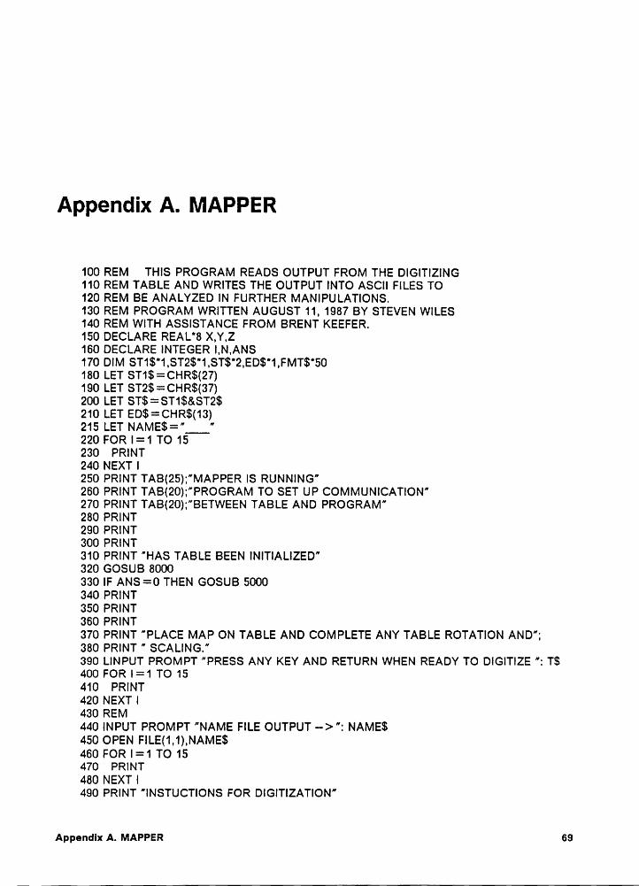
I

Appendux A. MAPPER

100 REM THIS PROGRAM READS OUTPUT FROM THE DIGITIZING110 REM TABLE AND WRITES THE OUTPUT INTO ASCII FILES TO120 REM BE ANALYZED IN FURTHER MANIPULATIONS.130 REM PROGRAM WRITTEN AUGUST 11, 1987 BY STEVEN WILES140 REM WITH ASSISTANCE FROM BRENT KEEFER.150 DECLARE REAL*8 X,Y,Z160 DECLARE INTEGER I,N,ANS170 DIM ST1$'1,ST2$'1,ST$"2,ED$'1,FMT$’50180 LET ST1$=CHR$(27)190 LET ST2$=CHR$(37)200 LET ST$=ST1$&ST2$210 LET ED$=CHR$(13)215 LET NAME$="__"220 FOR I=1 TO 15230 PRINT240 NEXT I250 PRINT TAB(25);"MAPPER IS RUNNING"260 PRINT TAB(20);”PROGRAM TO SET UP COMMUNICATION"270 PRINT TAB(20);"BETWEEN TABLE AND PROGRAM”280 PRINT290 PRINT300 PRINT310 PRINT "HAS TABLE BEEN INITIALIZED"320 GOSUB 8000330 IF ANS=0 THEN GOSUB 5000340 PRINT350 PRINT360 PRINT370 PRINT "PLACE MAP ON TABLE AND COMPLETE ANY TABLE ROTATION AND";380 PRINT " SCALING.”390 LINPUT PROMPT "PRESS ANY KEY AND RETURN WHEN READY TO DIGITIZE ": T$400 FOR I=1 TO 15410 PRINT420 NEXT I430 REM440 INPUT PROMPT "NAME FILE OUTPUT ··> ": NAME$450 OPEN FILE(1,1),NAME$460 FOR I=1 TO 15470 PRINT480 NEXT I

i 490 PRINT "INSTUCTIONS FOR DIGITIZATION"Appandix A. MAPPER 69

I

I

I

500 PRINT "POINT TO BE DIGITIZED IS WRITTEN ON DISPLAY." I510 PRINT "FIRST ENTER THE Z VALUE (ELEVATION)"520 PRINT "SECOND PLACE CURSOR OVER POINT AND PRESS ANY KEY." I530 PRINT I540 PRINT ""' TO SET Z VALUE USE EITHER"550 PRINT " ·CURSOR,FFFD____E"560

PRINT " -MENU, Z DATA FACTOR__CR" I570 PRINT " IT IS NOT NECESSARY TO BUFFER WITH ZEROS."580 PRINT590 PRINT ""' TO FINISH ENTERING DATA USE Z VALUE OF 9999."600 PRINT610 PRINT615 ENABLE HANDLER CLOSE,RESUME AT 800620 OPEN F|LE(2,0),"@TABLE"630 PRINT FILE(2),ST$;"M ";ED$640 PRINT "POINT COORDINATES "650 PRINT "NUMBER X Y Z"660 LET N=0670 PRINT FILE(2),ST$;"M DEFINE Z, THEN DIGITIZE #";N;ED$680 INPUT F|LE(2),X,Y,Z685 IF Z=9999 THEN GOTO 740690 LET I=IvIT$=”%%%% #,###.### #.###.### #.###”695 LET N = N +1700 PRINT USING FMT$:N,X,Y,Z710 PRINT FILE(1),X;",";Y;",";Z720 GOTO 670740 CLOSE750 PRINT760 PRINT770 PRINT "PROGRAM ENDED NORMALLY"780 PRINT "OUTPUT WRITTEN TO FILE ··> ";NAME$790 REM800 DISABLE HANDLER850 PRINT860 PRINT870 PRINT "DO YOU WANT TO DIGITIZE ANOTHER MAP?"880 GOSUB 8000890 IF ANS=1 THEN GOTO 340900 STOP901 REM902 REM5000 REM THIS SUBROUTINE SETS UP COMMUNICATIONS BETWEEN5010 REM TABLE DIGITIZER, DATA GENERAL, AND OUTPUT FILE5020 REM PROGRAM WRITTEN AUGUST 11, 1987 BY STEVE WILES5030 REM WITH ASSISTANCE FROM BRENT KEEFER.5040 FOR I=1 TO 15 I6060 PRINT I5060 NEXT I5070 PRINT " TABLE FORMATTOR AND COMMUNICATIONS SET·UP"5080 PRINT I5090 PRINT "FORMAT IS SET TO F8.0 FOR X AND Y COORDINATES";5100 PRINT ", AND F5.0 FORZ."5110

PRINT5120 PRINT "** LOCATE LOWER LEFT CORNER OF LARGE MENU II"5130 OPEN FILE(2,0),”@TABLE” I5135 PRINT FILE(2),ST$;"D1”;ED$

IAppendix A. MAPPER 70

I

5140 PRINT FILE(2),ST$;"F XF8.0,N2C,YF8.0,N2C,ZF5.0,NOD”;ED$5150 PRINT FILE(2),ST$;"VL”;ED$5160 CLOSE FILE(2)5170 FOR I=1 TO 85180 PRINT5190 NEXT I5200 RETURN5210 REM8000 REM SUBROUTINE TO RETURN A YES OR NO ANSWER8010 REM8015 LET ANS=38020 INPUT PROMPT "ANSWER EITHER Y OR N ·->": ANS$8030 IF ANS$=”Y" THEN LET ANS=18035 IF ANS$="y” THEN LET ANS=18040 IF ANS$="N” THEN LET ANS=08045 IF ANS$="n" THEN LET ANS=08050 IF ANS=3 THEN GOTO 80208060 RETURN8070 REM8500 HANDLER CLOSE8510 REM CLOSES ALL FILES INCASE OF ABORT ENDING8520 PRINT "ABNORMAL ENDING, CHECK DATA TYPE.”8530 PRINT ”OUTPUT FILE -—>";NAME$;" MAY HAVE DATA."8540 CLOSE8550 PRINT ”ERROR ON LINE";EXLINE8560 PRINT ”ERROR CODE”;EXTYPE8570 RESUME8580 REM9000 END

Appendix A. MAPPER 71

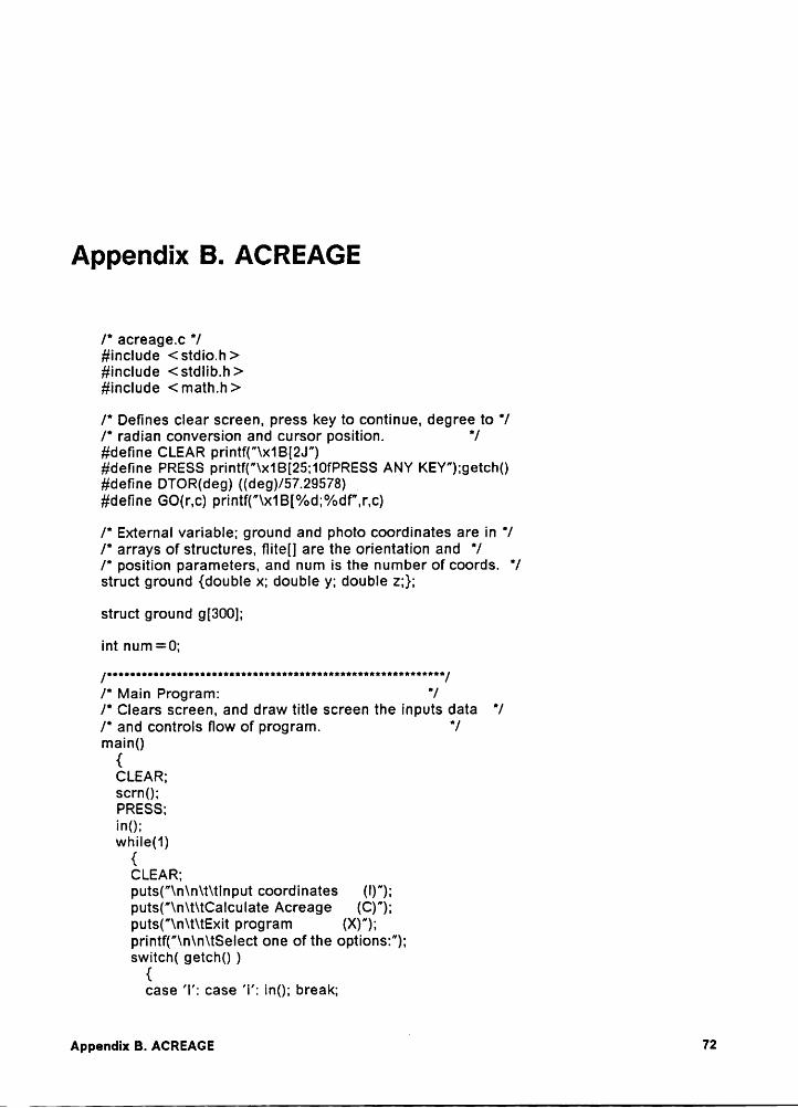
I

III

Appendix B. ACREAGE

/* acreage.c "/#include <stdio.h>#incIude <stdlib.h>#include < math.h >/* Detines clear screen, press key to continue, degree to "//* radian conversion and cursor position. "/#deline CLEAR printf("\x1B[2J")#define PRESS printf("\x1B[25;10fPRESS ANY KEY");getch()#detine DTOR(deg) ((deg)/57.29578)#detine GO(r,c) printf(”\x1B[°/>d;%df",r,c)

/* External variable; ground and photo coordinates are in *//' arrays of structures, fIite[] are the orientation and *//" position parameters, and num is the number of coords. */struct ground {double x; double y; double 2;};

struct ground g[300];

int num =0;

/° Main Program: '//* Clears screen, and draw title screen the inputs data '//* and controls llow of program. */main(){

CLEAR;scrn(); IPRESS; Iml);while(1) I{CLEAR; I

puts(”\n\n\t\tlnputcoordinates (l)”);puts("\n\t\tCalcuIate Acreage (C)"); Iputs("\n\t\tExit program (X)”);printf(”\n\n\tSeIect one of the optionsz"); Iswitch( getch() )

{ Icase ’l’: case ’i’: in(); break; I

I IAppendix B. ACREAGE 72

I

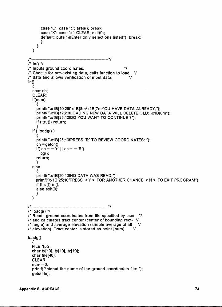
I

I

case ’C’:case ’c': area(); break; I

case 'X’: case ’x’: CLEAR; exit(0);default: puts("\nEnter only selections listed”); break;}}}

/* ln() '//* Inputs ground coordinates. "//' Checks for pre-existing data, calls function to load '//' data and allows verification of input data. "/ln()

<char ch;CLEAR;if(num){

printf("\x1B[10;25f\x1B[5m\x1B[7mYOU HAVE DATA ALREADY,");printf("\x1B[12;20fLOADING NEW DATA WILL DELETE OLD: \x1B[0m");printf(”\><1B[25;10fDO YOU WANT TO CONTINUE ?");if (Itru()) return;}

if( Ioadg() ){printf("\x1B[25;10fPRESS ’R’ TO REVIEW COORDINATES: ");ch =getch();if( ch= =’r’ || ch= =’R’)

pgll;return;}

else{printf("\x1B[20;10fNO DATA WAS READ,");printf("\x1B[25;10fPRESS <Y> FOR ANOTHER CHANCE < N> TO EXIT PROGRANI");if (tru()) in();else exit(0);}}

/‘*-—--—----—---—--·-—-----—-——-·—--—-·"//" Ioadg() '//° Reads ground coordinates from file specified by user *//° and calculates tract center (center of bounding rect- "//' angle) and average elevation (simple average of all '//* elevation). Tract center is stored as point [num] */

loadgO{FILE 'fptr;char tx[10], ty[10], tz[10];char file[40];CLEAR;num =0;printf(”\nInput the name of the ground coordinates file: ");gets(fiIe);

Appendix B. ACREAGE 73

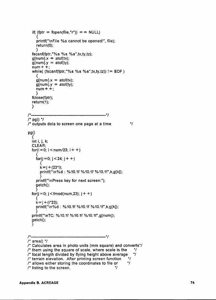
ll

if( (fptr = fopen(file,"r”)) = = NULL){printf(”\nFile %s cannot be openedl", file);return(0);}

fscanf(fptr,"°/>s %s %s”,t><,ty,tz);g[num].x = atof(tx);g[num].y = atof(ty);num + +;while( (fscanf(fptr,"%s %s %s",tx,ty,tz)) != EOF ){

g[num].x = atof(tx);g[num].y = atof(ty);num + +;}

fclose(fptr);return(1);}

/'··----·—-··-·-·-···-·~—···-——·-··-··-·-·~·······'//* pol) '//* outputs data to screen one page at a time '/

vgl){int i, j, k;CLEAR;for(i=0; i<num/23; i+ +){

for(j=0; j<24; j+ +){k=j+(23"i);printf(”\n°/od : %10.1f %10.1f %10.1f",k,g[k]);}

printf(”\nPress key for ne><t screenz");getch();}

for(j=0; j<fmod(num,23); j+ +){k=j+(i"23);printf(”\n°/>d : %10.1f %10.1f %10.1f^',k,g[k]);}

printf("\nTC: %10.1f %10.1f %10.1f",g[num]);getch();}

/° area() °//° Calculates area in photo units (mm square) and converts°/ i/' them using the square of scale, where scale is the '/ j/' focal length divided by flying height above average */ L/' terrain elevation. After printing screen function *//* allows either storing the coordinates to file or '/

Ä

/" listing to the screen. "/

Appendlx B. ACREAGE 74

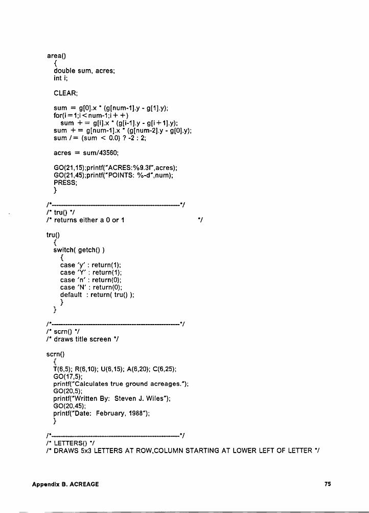
area(){double sum, acres;int l;

CLEAR;

Sum = Qlül->< ' l¤l¤¤m·1l-v · 9l1l-v):for(i =1;i < num-1;i + +)

Sum + = dll}->< ' lQl¤—1l-v · Ql¤+1l-v):sum + = g[num-1].x * (g[num-2].y · g[0].y);sum /= (sum < 0.0) ? -2: 2;

acres = sum/43560;

GO(21,15);printf(”ACRES:%9.3f",acres);GO(21,45);printf("POINTS: %-d",num);PRESS;}

. /' tru() '//* returns either a 0 or 1 °/

tru(){switch( getch() ){

case ’y’ : return(1);case ’Y’ : return(1);case ’n’ : return(0);case ’N’ : return(0);default : return( tru() );}}

/' scrn() °//' draws title screen */

scrn(){T(6,5); R(6,10); U(6,15); A(6,20); C(6,25);GO(17,5);printf("Calculates true ground acreages/');GO(20,5);printf("Wrltten By: Steven J. Wiles");GO(20,45);printf("Date: February, 1988");}

/* LETTERS() '//" DRAWS 5x3 LETTERS AT ROW,COLUMN STARTING AT LOWER LEFT OF LETTER */

Ä

Appendix B. ACREAGE 75

A(r,c)int r,c;{

GO((r-4),c); printf("\xC9\xCD\xBB");GO((r-3),c); printf("\xBA\xFF\xBA”);GO((r—2),c); printf(”\xCC\xCD\xB9");GO((r·1),c); printf("\xBA\xFF\xBA");GO(r,c); printf("\xD0\><FF\xD0");}

C(r,c)int r,c;{

GO((r-4),c); printf("\><C9\xCD\xB8”);GO((r·3),c); printf("\xBA\><FF\xFF”);GO((r—2),c); printf("\xBA\xFF\xFF");GO((r-1),c); printf("\xBA\xFF\><FF");GO(r,c); printf("\xC8\xCD\xBE");}

E(r,c)int r,c;{

GO((r-4),c); printf("\xC9\xCD\xCD");GO((r-3),c); printf("\xBA\xFF\xFF”);GO((r—2),c); printf("\xCC\xCD\xFF”);GO((r·1),c); printf("\xBA\xFF\xFF");GO(r,c); printf(”\xC8\xCD\xCD");}

G(r,c)int r,c;{

GO((r-4),c); printf("\xC9\xCD\xB8");GO((r·3),c); printf("\xBA\><FF\xFF");GO((r—2),c); printf(”\xBA\xC6\xBB”);GO((r-1),c); printf("\xBA\xFF\xBA");GO(r,c); printf("\xC8\xCD\xBC”);}

H(r,c)int r,c;{

GO((r·4),c); printf(”\><D2\xFF\xD2”);GO((r-3),c); printf("\xBA\xFF\xBA”);GO((r—2),c); printf("\xCC\xCD\xB9”);GO((r·1),c); printf("\xBA\xFF\><BA");GO(r,c); printf("\xD0\xFF\xD0");}

|(r,c)int r,c;{

GO((r-4),c); printf("\xFF\><D2\xFF");GO((r-3),::); printf("\xFF\xBA\xFF”);GO((r—2),c); printf(”\xFF\xBA\xFF");GO((r-1),c); printf("\xFF\xBA\><FF”);GO(r,c); printf("\xFF\xD0\xFF”);}

L(r,c)int r,c;

Appendix B. ACREAGE 76

{GO((r-4),c); printf("\xD2\xFF\xFF");GO((r·3),c); printf(”\xBA\xFF\xFF");GO((r-2),c); printf("\xBA\xFF\xFF");GO((r·1),c); printf(”\><BA\xFF\xFF");GO(r,c); printf("\xC8\xCD\xCD");}

M(r,c)int r,c;{

GO((r-4),c); printf("\xC9\xCB\xBB");GO((r-3),c); printf("\xBA\xBA\xBA");GO((r-2),c); printf("\xBA\><DO\xBA”);GO((r·1),c); printf(”\xBA\xFF\xBA”);GO(r,c); printf("\xD0\xFF\xD0");}

N<r„¤)int r,c;{

GO((r-4),c); printf("\xD6\xBF\xD2");GO((r-3),c); printf("\xBA\><B3\><BA");GO((r-2),c); printf("\xBA\xB3\xBA");GO((r·1),c); printf(”\xBA\xB3\xBA");GO(r,c); printf(”\xD0\xC0\xBD");}

O(r,c)int r,c;{

GO((r-4),c); printf(”\xC9\xCD\xBB");GO((r-3),::); printf("\><BA\xFF\xBA”);GO((r-2),c); printf(”\xBA\xFF\xBA");GO((r·1),c); printf("\><BA\xFF\xBA");GO(r,c); printf("\xC8\xCD\xBC");}

P(r,c)int r, c;{

GO((r-4),c); printf(”\xC9\xCD\xBB");GO((r-3),c); printf("\xBA\xFF\xBA”);GO((r—2),c); printf(”\xCC\xCD\><BC”);GO((r·1),c); printf("\><BA");GO(r,c); printf("\xD0");}

R(r,c)int r, c;{

GO((r-4),c); printf(”\xC9\xCD\xBB");GO((r-3),c); printf("\xBA\xFF\xBA");GO((r-2),c); printf("\><CC\xCB\xBC");GO((r·1),c); printf("\xBA\xC8\xBB");GO(r,c); printf("\xD0\xFF\xD0");}

S(r,c)int r,c;{

GO((r-4),c); printf(”\xC9\xCD\xB8");

Appandix B. ACREAGE 77

GO((r—3),c); printf("\xBA\xFF\><FF");GO((r·2),c); printf(”\><C8\xCD\xBB”);GO((r-1),c); printf("\xFF\xFF\xBA");GO(r,c); printf(”\xC6\xCD\xBC");}

T(r,c)int r,c;{

GO((r-4),c); printf("\xCD\xCB\xCD");GO((r-3),c); printf("\xFF\xBA\xFF");GO((r-2),c); printf("\xFF\xBA\xFF”);GO((r-1),c); printf("\xFF\xBA\xFF");GO(r,c); printf("\xFF\xD0\xFF");}

U(r,c)int r,c;{

GO((r-4),c); printf("\xD2\xFF\xD2");GO((r-3),c); printf("\xBA\xFF\xBA");GO((r·2),c); printf("\xBA\xFF\xBA");GO((r-1),c); printf("\xBA\xFF\xBA");GO(r,c); printf(”\xC8\xCD\xBC”);

Appendix B. ACREAGE 78

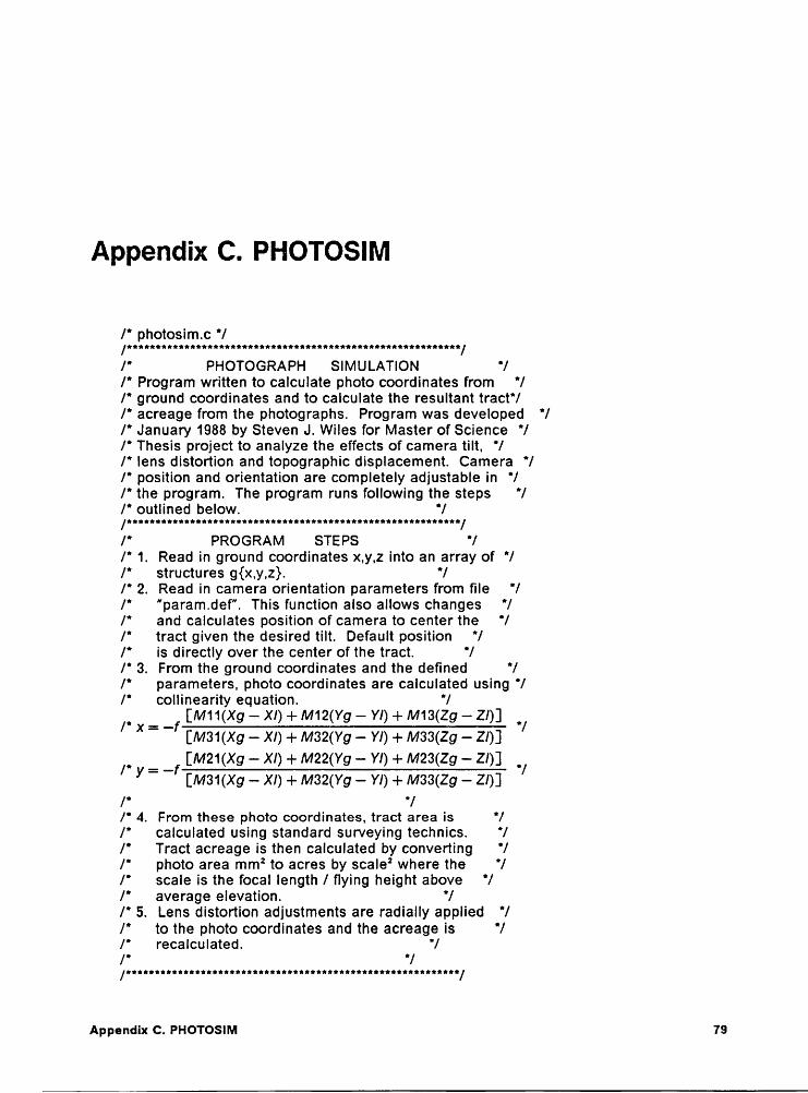
Appendix C. PHOTOSIM

/' photosim.c */

I" PHOTOGRAPH SIMULATION *//* Program written to calculate photo coordinates from "//* ground coordinates and to calculate the resultant tract'//* acreage from the photographs. Program was developed *//" January 1988 by Steven J. Wiles for Master of Science '/I" Thesis project to analyze the effects of camera tilt, */I" lens distortion and topographic displacement. Camera "/I' position and orientation are completely adjustable in */I" the program. The program runs following the steps *//* outlined below. °//QQtlttttthllthtlttttttillttltttQIQQQQQtilltttillllttlliltllI" PROGRAM STEPS °//" 1. Read in ground coordinates x,y,z into an array of 'II" structures g{x,y,z}. 'I/‘ 2. Read in camera orientation parameters from file *//* "param.def”. This function also allows changes 'I/* and calculates position of camera to center the '//" tract given the desired tilt. Default position *//* is directly over the center of the tract. '//" 3. From the ground coordinates and the defined *//" parameters, photo coordinates are calculated using "/I" collinearity equation. "//_

f[Il//11(Xg—XI)+Il//12(Yg— YI) +M13(2g—Z/)] _/

X [M31(Xg — XI) + /V/32(Yg — YI) + M33(2g — 2/)]/_

f [A/l21(Xg — XI) + M22(Yg — YI) + M23(2g — 2/)] _/y —

[M31(Xg — XI) + M32(Yg — YI) + /l/I33(2g — 2/)]/* *//* 4. From these photo coordinates, tract area is *//' calculated using standard surveying technics. '//* Tract acreage is then calculated by converting '/I' photo area mm! to acres by scale’ where the "/I" scale is the focal length / flying height above '//" average elevation. */I" 5. Lens distortion adjustments are radially applied '//* to the photo coordinates and the acreage is *//' recalculated. '//° */

Appendix C. PHOTOSIM 79

/° Libraries for input/output and higher level math */#include <stdio.h>#include <stdIib.h>#include < math.h >

/* Defines clear screen, press key to continue, degree to *//* radian conversion and cursor position. */#detine CLEAR printf("\x1B[2J”)#detine PRESS printf("\x1B[25;10fPRESS ANY KEY");getch()#detine DTOR(deg) ((deg)/57.29578)#deline GO(r,c) printf("\x1B[°/¤d;%df",r,c)

/° External variable; ground and photo coordinates are in '//' arrays of structures, tlite[] are the orientation and */ ‘/* position parameters, and num is the number of coords. */struct ground {double x; double y; double 2;};struct photo {double x; double y;};

struct ground g[300];struct photo p[300];

double flite[8];int num =0;/lIll!QtRQQQQQttt!QttIItltlhQIIlllltlttt*!QthItI•I|ItI••Itt//* Main Program: *//" Clears screen, and draw title screen the inputs data "//" and controls tlow of program. */main(){

CLEAR;scrn();PRESS;l¤<);while(1){

CLEAR;puts("\n\n\t\tlnput coordinates (|)");puts("\n\t\tRun Simulation (S)”);puts(”\n\t\tExit program (X)");printf("\n\n\tSelect one of the optionsz");switch( getch() )

<case ’l’: case ’i’: in(); break;case ’S’: case ’s’: runl); break;case

’X’:case

’x’:CLEAR; exit(0);

default: puts("\nEnter only selections listed"); break;}}}

/' in() *//" Inputs ground coordinates. '//* Checks for pre-existing data, calls function to load '/

Appendlx C. PHOTOSIM 80

/' data and allows verification of input data. */in(){

char ch;CLEAR;if(num){

printf("\x1B[10;25f\x1B[5m\x1B[7mYOU HAVE DATA ALREADY,”);printf("\x1B[12;20fLOADlNG NEW DATA WILL DELETE OLD:\x1B[0m");printf("\x1B[25;10fDO YOU WANT TO CONTINUE ?");if (!tru()) return;}

if( Ioadg() ){printf("\x1B[25;10fPRESS ’R’ TO REVIEW COORDlNATES:");ch=getch();if( ch= =’r’ || ch= =’R')pal);return;}

else{printf("\x1B[20;10fNO DATA WAS READ,”);printf("\x1B[25;10fPRESS <Y> FOR ANOTHER CHANCE < N > TO EXIT PROGRAM");if (tr¤0) int);else exit(0);}}

/" run() '//' Calls functions to define parameters, run simulation "//* and output results to screen and data to file or screen'!

run(){Int i=0;if(num < 1){

puts("No data entered");PRESS;return;}

deüne0;slm();area(”No\0");

wl2ile(1)

CLEAR;puts("\n\n\t\tChange Parameters (P)”);puts("\n\t\tLens Distortlon (L)");puts(”\n\t\tMain Menu (M)");printf("\n\n\t\tSelect one of the options:”);swItch( getch() )

Appendix C. PHOTOSIM 81

{case ’P’: case ’p':

i=0;deüneO;sim();area("No\0");break;

case ’L’: case 'I':if(i){

CLEAR;printf(”\x1B[10;15f\x1B[5m\x‘IB[7m");

printf("YOU HAVE ALREADY ADJUSTED FOR LENS DlSTORTlON\x1B[0m”);printf(”\x1B[25;10fDO YOU WANT TO CONTINUE ?");if (!tru()) break;}

Iens();i+ +;if (i < 2) area("Yes\0");else area(”Dbl\0”);break;case 'M': case 'm’: return;

. default : puts(”Enter option listed"); PRESS;}}}

/* define '//* Reads camera orientation from file and position form '//" load() tract center calculation. All parameters are *//* adjustable and by typing ’c’ the tract is centered to "//' acount for tilt of the camera. */

deüne0{char temp[10], temp1;int change, i;double offset;FILE "param;

if( (param=fopen("param.def","rb")) != NULL){for(i =0;i <8;i+ +) fread(&flite[i],sizeof(fiite[i]),1,param);fclose(param);}

fiite[5]=g[num].x;flite[6]=g[num].y;

do { ICLEAR; IGO(2,15);printf("1. Focal Length:%-6.2f",flite[0]);GO(4,15);printf("2.Tilt :%-6.2f",flite[1]);GO(6,15);printf(”3. Swing :%—6.2f",fiite[2]);GO(8,15);printf("4. Azimuth :%-6.2f",fiite[3]);

Appendix C. PHOTOSIM 82 I

GO(10,15);printf("5. Flying Height : %·9.2f",flite[4]);GO(12,15);printf(”6. Exposure X :°/>-9.2f",flite[5]);GO(14,15);printf(”7. Exposure Y :%-9.2f”,flite[6]);GO(16,15);printf(”8. Relief Factor: %4.2f”,flite[7]);

GO(20,10);printf("Type parameter to be changed <1-8> or <return>");GO(21,10);printf("Type c for tilt auto centerlng\n\n");temp1=getch();

if(temp1>’0’

&& temp1< ’9’){change=atol(&temp1);GO((change*2),45);printf("New = > ");getsltemp); tlite[change—1]=atof(temp);}

if(temp1= = 'c’){offset = flite[4]*tan( DTOR(flite[1]) );llite[5] = g[num].x + offset'sin( DTOR(llite[3]—l-180) );tlite[6] = g[num].y + offset'cos( DTOR(llite[3]+180) );}}

whiIe(temp1!=’\r’);

param=fopen("param.def","wb");fwrite(flite,sizeof(flite[0]),8,param);fcIose(param);}

/* sim() *//* Calculates photo coordinates from ground data and *//' camera orientation and position parameters. '//* Collinearity equations are from Wolf, P. R. 1983 '//' Elements of Photogrammetry. '/

sim(){int i, out=0;double ct, cs, ca, st, ss, sa;double m11, m12, m13, m21, m22, m23, m31, m32, m33;double ht, xnum, ynum, deno;double a, b, c, eIev[300];

CLEAR;P(16,25); H(16,30); O(16,35); T(16,40); O(16,45);

ct=cos( DTOR(flite[1]) );cs=cos( DTOR(flite[2]) );ca=cos( DTOR(flite[3]) );st=sin( DTOR(flite[1]) );ss=sin( DTOR(flite[2]) );sa=sin( DTOR(flite[3]) );m11=·ca*cs·sa*ct*ss;

Appendix C. PHOTOSIM 83

m12 =sa*cs-ca"ct*ss;1m13=-st*ss;m21=ca'ss·sa"ct"cs;m22 =-sa'ss·ca"ct'cs;m23=-st*cs;m31=-sa*st;m32=·ca'st;m33=ct;

for(i=0;i < =num;i+ +)elev[i] =g[i].z*fiite[7];

ht=flite[4]+elev[num];

for(i=0;i < =num;i+ +){a =g[i].x-fIite[5];b=9[I]-Y-fIite[6];c=eIev[i]-ht;xnum=m11"a+m12'b+m13*c;ynum = m21*a + m22*b + m23*c;deno=m31*a+m32*b+m33*c;p[i].x=-fIite[0]*xnum/deno;p[i].y=-fIite[0]*ynum/deno;gl lplil-><'¤liI-><>+<¤lii-v'¤lil.v> > 468 ) <>¤t+ +:

iüouü{GO(6,23);printf("Results may be incorrectl");GO(9,20);printf("°/od points were off photograph”,out);PRESS;}}

/* Ioadg() "//* Reads ground coordinates from file specified by user "//' and calculates tract center (center of bounding rect- "//" angle) and average elevation (simple average of all *//* elevation). Tract center is stored as point [num] */

lo?dg0

FILE *fptr;char tx[10], ty[10], tz[10];char file[40];double maxx, minx, maxy, miny, sumz;CLEAR;num =0;printf(”\nInput the name ofthe ground coordinates file: ");gets(üIe);

if( (fptr = fopen(file,"r")) = = NULL){printf(”\nFile °/es cannot be openedl", file);return(0);}

Appendix C. PHOTOSIM 84

fscanf(fptr,"%s °/os %s",tx,ty,tz);maxx = minx = g[num].x = atof(tx);maxy = miny = g[num].y = atof(ty);sumz = g[num].z = atof(tz);num + +;whi|e( (fscanf(fptr,"°/os %s %s",tx,ty,tz)) != EOF ){

g[num].x = atof(tx);g[num].y = atof(ty);sumz + = g[num].z = atof(tz);if(g[num].x> maxx) maxx=g[num].x;if(g[num].x<minx) minx=g[num].x;if(g[num].y>maxy) maxy=g[num].y;if(g[num].y<miny) miny=g[num].y;num + +;}

fclose(fptr);g[num].x = (minx+maxx)/2;g[num].y = (miny+maxy)/2;g[num].z = sumz/num;return(1);}

/'·---·-·-—-—--·-·-·~·—-···—-··-·····--·····-·-··"//' ngt) '//" outputs data to screen one page at a time "/

ngt){int i, j, k;CLEAR;for(i=0; i<num/23; i+ +){

for(j=0; j<24; j+ +){k=j+(23*i);printf(”\n%d : %10.1f %10.1f %10.1f",k,g[k]);}

printf("\nPress key for next screenx");getch();}

for(j =0; j<fmod(num,23); j+ +){k=j+(i*23);printf("\n°/od : %10.1f %10.1f %10.1f”,k,g[k]);}

printf(”\nTC: %10.1f %10.1f %10.1f”,g[num]); Igetch(); I} i

I/‘ p¤0 '/ _/* outputs data to screen one page at a time */

ppt){

Appendix C. PHOTOSIMA

85I

I

Int i, j, k;CLEAR;for(i=O; i<num/23; i+ +){

f0r(j=0; j<24; j+ +){k=j +(23*i);printf(”\n%d : %10.4f %10.4f",k,p[k]);}

printf("\nPress key for next screenz");getch();}

for(j=0; j<fmod(num,23); j+ +){k=j+(i*23);printf("\n%d : %10.4f %10.4f",k,p[k]);}

printf("\nTC: %10.4f %10.4f",p[num]);getch();}

/°·------···-—·-·····--··-··-—-·-·—·—···--—-··*//° odata() '//* outputs photo coordinates in ASCII format to file '//* entered at output screen in function area(). °//* The last point Is the tract center and ave elev. '/

odata(file)char file[40];{

FILE *out;int I;CLEAR;if(Inum)

{puts("\x1B[10;25fNo data to write to file.");return;}

if( (out=fopen(file,"w")) = =NULL ){printf("\x1B[10;25fFile %s cannot be opened.",file);return;}

for(i=0;i < =num;i + +) fprintf(out,"%f %f\n",p[i]);fclose(out);}/"··-··---*//‘ area() "//" Calculates area in photo units (mm square) and converts'//* them using the square of scale, where scale is the *//* focal length divided by flying height above average '//' terrain elevation. After printing screen function "//" allows either storing the coordinates to file or *//* listing to the screen. "/ I

Appandlx C. PHOTOSIM 86

1

1

1

1area(lensd) 1char lensd[4];{

double sum, scale, psr2, acres;int l;char ch, name[40];

CLEAR;

Sum = ¤l0l~>< ' l¤l¤¤m·1l-v - ¤l1l-v):for(i=1;i <num·1;i+ +)Sum + = plil->< ' (PÜ·1]·Y · vll +11.v):sum + = p[num-1].x * (p[num-2].y - p[0].y);sum /= (sum < 0.0) ? -2: 2;

scale = flite[0]/llite[4];psr2=1/(scaIe*scaIe);acres = (sum'psr2)/43560;

GO(10,15);printf("T|LT: %6.2f deg",flite[1]);GO(9,45);printf("HEIGHT: %5.0f ft”,t1ite[4]);GO(12,15);printf("SWlNG: %6.2f deg",tlite[2]);GO(11,45);printf(”LENS: %6.2fmm",t1ite[0]);GO(14,15);printf("AZIlvlUTH:%6.2f deg”,flite[3]);GO(13,45);printf(”DlST: %s",Iensd);GO(15,45);printf(”RELIEF: %4.2f",flite[7]);GO(19,15);printf("NlM’: %7.3f",sum);GO(19,45);printf("SCALE 12%-.0f”,(304.8/scale));GO(21,15);printf(”ACRES:%9.3f",acres);GO(21,45);prlntf(”POINTS: %-d”,num);GO(05,15);printf("FlLE NAME:");

gets(name);GO(25,10);printf("PRESS ’F’ TO FlLE COORDINATES: ”);ch=getch();if (ch= =’f'

ll ch= =’F')odata(name);

GO(25,10);printf("PRESS ’S’ FOR SCREEN LISTING: ");ch =getch();if (ch= =’s’

|| ch= =’S’)1¤¤0;}

/* tru() °/ 1/* returns either a 0 or 1 */ I

tru() I{ . lsw1tch( getch() ){

case ’y’ : return(1); Icase

’Y’: return(1); 1

case 'n’: return(0);

case ’N' : return(0); 1default : return( tru() );

I

Appendlx C. PHOTOSIM87I

I

I

I

I— I

}}

/* lens() *//" calculates and adjusts for lens distortions */

lens(){double r, r3, r5, r7, d;int i;

CLEAR;L(16,25); E(16,30); N(16,35); $(16,40);

for(i =0;i <num;i + +){r=S¤r1( ¤¤w(¤lil.><„2) + ¤¤w(¤lil-v.2) i:r3 = pow(r,3);r5 = pow(r,5);r7 = pow(r,7);

d = (r'-5.967984) + (r3'0.0280528) + (r5'0.000194025) + (r7*-7.09349E·07);d /= 1000.0;

p[i].x '= (1 +d/r);plil-v '= (1 +d/r);}}

/* scrn() °//* draws title screen */

I scrn(){P(6,5); H(6,10); O(6,15); T(6,20); O(6,25);G(6,30); R(6,35); A(6,40); P(6,45); H(6,50);$(13,5); l(13,10); M(13,15); U(13,20); L(13,25);A(13,30); T(13,35); O(13,40); R(13,45);camera(11,55);GO(17,5);printf(”CalcuIates photo coordinates from ground coordinates.");GO(18,5);printf("Camera position and orientation are adjustable.");GO(20,5);printf(”Written By: Steven J. Wiles");GO(20,45);printf("Date: January, 1988”);}

!!·•··-·-·.•__•-X-•I’/" LETTERS() *//* DRAWS 5x3 LETTERS AT ROW,COLUMN STARTING AT LOWER LEFT OF LETTER "/

A(r,c)

Äint r,c;

TAppendix C. PHOTOSIM 88

{GO((r-4),0); printf("\xC9\xCD\xBB");GO((r-3),c); printf(”\xBA\xFF\xBA");GO((r-2),c); printf("\xCC\xCD\xB9”);GO((r-1),c); printf(”\xBA\xFF\xBA”);GO(r,c); printf(”\xD0\xFF\xD0");}

E(r,c)int r,c;{

GO((r-4),c); printf("\xC9\xCD\xCD");GO((r-3),c); printf("\xBA\xFF\xFF”);GO((r-2),c); printf("\xCC\xCD\xFF");GO((r-1),c); printf(”\xBA\xFF\xFF");GO(r,c); printf("\xC8\xCD\xCD");}

G(r,c)int r,c;{

GO((r-4),c); printf("\xC9\xCD\xB8");GO((r-3),c); printf("\xBA\xFF\xFF");GO((r-2),c); printf("\xBA\xC6\xBB”);

.„ GO((r-1),c); printf("\xBA\xFF\xBA”);GO(r,c); printf(”\xC8\xCD\xBC”);}

H(r.<=)int r,c;{

GO((r-4),c); printf("\xD2\xFF\xD2");GO((r-3),c); printf("\xBA\xFF\><BA”);GO((r-2),c); printf("\xCC\xCD\xB9");GO((r·1),c); printf(”\xBA\xFF\xBA");GO(r,c); printf("\xD0\xFF\xD0”);}

I(r,c)int r,c;{

GO((r-4),c); printf(”\xFF\xD2\xFF");GO((r-3),0); printf(”\xFF\xBA\xFF”);GO((r-2),c); printf(”\xFF\xBA\><FF");GO((r-1),c); printf("\><FF\xBA\xFF”);GO(r,c); printf("\xFF\xD0\xFF”);}

L(r,c)int r,c;{

GO((r·4),c); printf("\xD2\xFF\xFF");GO((r—3),c); printf("\xBA\xFF\xFF");GO((r-2),c); printf("\xBA\xFF\xFF");GO((r·1),c); printf("\xBA\xFF\xFF");GO(r,c); printf("\xC8\xCD\xCD”);}

M(r,c)int r,c;{

GO((r-4),c); printf(”\xC9\xCB\xBB");

Appandlx C. PHOTOSIM 89

GO((r-3),c); printf("\xBA\xBA\xBA");GO((r—2),c); printf(”\><BA\xD0\xBA”);GO((r·1),c); printf("\xBA\xFF\xBA");GO(r,c); printf("\xD0\xFF\xD0”);}N<n¢)

int r,c;{GO((r·4),c); printf("\xD6\xBF\xD2”);GO((r-3),c); printf("\><BA\xB3\><BA”);GO((r—2),c); printf("\xBA\xB3\xBA");GO((r·1),c); printf("\xBA\xB3\xBA");GO(r,c); printf("\xD0\xC0\xBD");}

O(r,c)int r,c;{

GO((r·4),c); printf("\xC9\xCD\xBB”);GO((r-3),c); printf("\xBA\xFF\xBA");GO((r·2),c); printf("\xBA\xFF\xBA");GO((r·1),c); printf(”\xBA\xFF\xBA");GO(r,c); printf(”\xC8\xCD\xBC”);}

P<r.¤)int r, c;{

GO((r·4),c); printf("\xC9\xCD\xBB");GO((r-3),c); printf("\xBA\xFF\xBA");GO((r—2),c); printf("\xCC\xCD\xBC”);GO((r·1),c); printf(”\xBA”);GO(r,c); printf("\xD0");}

R(r,c)int r, c;{

GO((r·4),c); printf("\xC9\xCD\xBB");GO((r-3),c); printf("\xBA\xFF\xBA");GO((r—2),c); printf(”\><CC\xCB\xBC”);GO((r·1),c); printf(”\xBA\xC8\xBB");GO(r,c); printf(”\xD0\xFF\xD0”);}S<r.c)

int r,c;{GO((r·4),c); printf("\xC9\xCD\xB8");GO((r-3),c); printf(”\><BA\xFF\xFF");GO((r—2),c); printf("\xC8\xCD\xBB");GO((r·1),c); printf(”\xFF\xFF\xBA”);GO(r,c); printf(”\xC6\><CD\xBC”);}

T(r,c)int r,c;{

GO((r·4),c); printf("\xCD\xCB\><CD”);GO((r-3),c); printf(”\xFF\><BA\xFF");GO((r—2),c); printf(”\xFF\xBA\xFF”);

Appandix C. PHOTOSIM 90

111

GO((r-1),c); printf("\xFF\xBA\xFF");GO(r,c); printf("\xFF\xD0\xFF”);}

U(r,c)int r,c;{

GO((r-4),c); printf("\xD2\xFF\xD2");GO((r·3),c); printf("\><BA\xFF\xBA");GO((r·2),c); printf("\><BA\xFF\xBA");GO((r-1),c); printf("\xBA\xFF\xBA");GO(r,c); printf("\xC8\xCD\xBC");}

camera(r,c)int r,c;{G¤<(r-4).c);printf("\xFF\xFF\xFF\xFF\xD6\xC4\xC4\xC4\xC4\xC4\xB7\xFF\xFF\xFF\xFF”);

GO((r—3),c);printf(”\xC9\><CD\xCD\xCD\xBC\xFF\xAE\x99\xAF\xFF\xC8\xCD\xCD\xCD\xBB");

GO((r·2),c);printf("\xBA\xB0\xB0\xFF\xFF\xFF\xDE\xDB\xDD\xFF\xFF\xFF\xB0\xB0\xBA");

GO((r-1),c);printf("\xBA\xB0\xB0\xFF\xFF\xFF\xFF\xFF\xFF\xFF\xFF\><FF\xB0\xB0\xBA");

GO(r,c);printf("\xC8\xCD\xCD\xCD\xCD\xCD\xCD\xCD\xCD\xCD\xCD\xCD\xCD\xCD\xBC");

Appandix C. PHOTOSIM 91

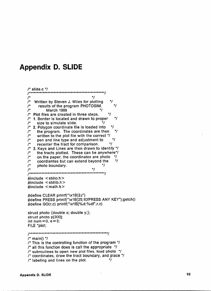
Appendix D. SLIDE

/" slide.c */

/° *//* Written by Steven J. Wiles for plotting '//° results ofthe program PHOTOSIM. *//" March 1988 *//* Plot files are created in three steps. '//* 1. Border is located and drawn to proper *//" size to simulate slide. *//* 2. Polygon coordinate file is loaded into °//* the program. The coordinates are then °//* written to the plot file with the correct */ ‘ ‘·/* pen and line type and adjustment to '//" recenter the tract for comparison. '//* 3. Keys and Lines are then drawn to identify '//" the tracts plotted. These can be anywhere'//* on the paper, the coordinates are photo '//* coordiantes but can extend beyond the *//* photo boundary. '//* *//IltitthIttQIQtttltitltltttitlttllttltlttltlttttttl#include <stdio.h>#include < stdlib.h >#include < math.h >

#define CLEAR printf("\x1B[2J")#define PRESS printf("\x1B[25;10fPRESS ANY KEY");getch()#define GO(r,c) printf("\x1B[%d;%df",r,c)

struct photo {double x; double y;};struct photo p[300];int num=0, e=3; IFILE *plot; I

/" main() '//* This is the controlling function of the program *//* all this function does is call the appropriate */ l/" subroutines to open new plot files, load photo "//" coordinates, draw the tract boundary, and place "/ °/° labeling and lines on the plot. */ °

Appendix D. SLIDE 92éI

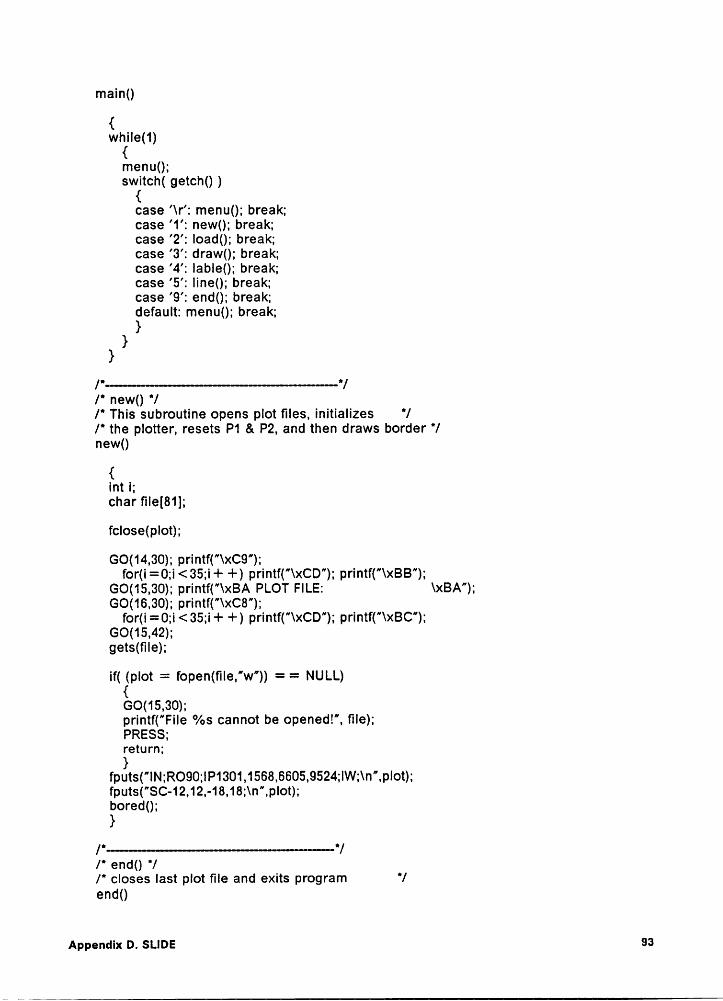
main()

{whiIe(1){

menu();switch( getch() ){

case ’\r’: menu(); break;case

’1’: neW(); break;case ’2’: loadl); break;case ’3’: draW(); break;case ’4': Iablel); break;case

’5’:linel); break;

case’9’: end(); break;

default: menu(); break;}}}

/* new() "//‘ This subroutine opens plot files, initializes '//* the plotter, resets P1 & P2, and then draws border */new()

{Int I;char file[81];

fcIose(plot);

GO(14,30); printf("\xC9");for(i=0;i <35;i+ +) printf("\xCD”); printf("\xBB”);

GO(15,30); printf("\><BA PLOT FILE: \xBA");GO(16,30); printf("\xC8");

for(i=0;l <35;i+ +) printf("\xCD"); printf("\xBC”);GO(15,42);gets(fiIe);

if( (plot = fopen(fi|e,"w")) = = NULL){GO(15,30);printf(”FiIe %s cannot be openedl", file);PRESS;geturn;

fputs("lN;RO90;lP1301,1568,6605,9524;lW;\n",pIot);fputs(”SC-12,12,-18,18;\n”,plot);bored();}

/*··-—·······-·-···-—······-·-·--··-·—···—·-——-°//° end() *//* closes last plot file and exits program */end()

, Appendix D. SLIDE 93

1

1

1

1{fclose(plot);CLEAR;exlt(0);}

/* menu() "//* Displays main menu showing available choices */menu(){

int I;CLEAR;$(10,5);L(10,12);I(10,19);D(10,26);E(10,33); ‘GO(13,5); printf("\xC9");

for(i=0;i <20;i+ +) printf("\xCD"); printf(”\xBB");GO(14,5); prlntf(”\xBA 1 = > NEW PLOT FILE \xBA”);GO(15,5); printf("\xBA 2 = > LOAD POLY FILE\xBA”);GO(16,5); prlntf("\xBA 3 = > DRAW POLYGON \xBA”);GO(17,5); printf("\xBA 4 = > DRAW LABELS \xBA”);GO(18,5); printf(”\xBA 5 = > DRAW LINES \xBA");GO(19,5); printf("\xBA 9 = > EXIT PROGRAM \xBA”);GO(20,5); printf("\xC8");

for(i=0;i <20;i+ +) printf(”\xCD"); printf("\xBC");

GO(13,30); printf(”\xC9");for(i=0;i<14;i+ +) printf("\xCD"); printf("\xBB");

GO(14,30); prlntf(”\xBA SELECT #2 \xBA");GO(15,30); printf("\xC8");

for(l=0;i<14;i+ +) printf("\xCD"); printf("\xBC");GO(14,41);}

/'·-——·-·······-·-·-—···—···-··--·—-····-····--"//° Ioad() *//' Ioads in the speciiied photo coordinates "/load(){

FILE "in;int i;char tx[10], ty[10];char liIe[81];

GO(14,30); printf("\xC9");for(i=0;i <30;i + +) printf("\xCD"); printf(”\xBB");

GO(15,30); printf("\xBA FILE: \xBA”);GO(16,30); printf("\xC8");

for(i=0;i <30;i+ +) printf("\xCD"); printf("\xBC");GO(15,37);gets(tlle);

num =0;if( (in = fopen(tile,”r")) = = NULL){

Appendix D. SLIDE 94

GO(15,30);printf(”FiIe %s cannot be opened!”, file);PRESS;return;}

whiIe( (fscanf(in,"%s %s',tx,ty)) l= EOF){p[num].x = atof(tx);p[num].y = atof(ty);num + +;}

num-;fclose(in);}

/" draw() *//* Subroutine to draw the simulated tract photograph °//* the window is set at the photograph border so that *//* points off of the photograph are nor piotted. *//" Pen number, line type, and center are available. *//" The centering option adjusts the tract coordiantes *//" so that the tract center and the photo principal point '//' coincide. '/draw(){

double xadj, yadj;int i;char pen,|t;

GO(14,30); printf("\xC9");for(i=0;i<10;i+ +) printf("\xCD”); printf("\xBB");

GO(15,30); printf("\xBA PEN #: \xBA");GO(16,30); printf(”\xC8”);

for(i=0;i <10;i+ +) printf("\xCD"); printf(”\xBC”);GO(15,38);pen =getche();

GO(15,30); printf("\xC9");for(i=0;i<10;l+ +) printf("\xCD"); printf("\xBB");

GO(16,30); printf("\xBA LlNE#: \xBA”);GO(17,30); printf("\xC8");

for(i=0;l <10;i+ +) printf(”\xCD"); printf("\xBC");GO(1S,38);lt=getche();

GO(16,30); printf("\xC9");for(i=0;i<14;i+ +) printf("\xCD"); printf("\xBB");

GO(17,30); printf(”\xBA CENTERING? \xBA");GO(18,30); printf("\xC8");

for(i=0;i <14;i+ +) printf("\xCD"); printf("\xBC");GO(17,43);

if( tru() ){xadj=p[num].x;

Appendix D. SLIDE 95

lelse< lxadj =yadj =0;l

fputs(”lW1301,1568,6605,9524;\n",plot);fprintf(p|ot,"SP%c;LT%c;\n",pen,It);fprlntf(p|ot,"PU%.3f,%.3f;\n",(p[0].x-xadj),(p[0].y-yadj));for(i =1;i < num;i + +)

/" Iable() '//' Pen number and character sizes are input to "//" allow keying plots of several tract on the *//" same page. °/

. labIe(){char pen, sh[10], sw[10], strlng[81], x[10], y[10];int i;

GO(14,30); printf("\xC9");for(i=0;i<20;i+ +) printf(”\xCD"); printf("\xBB");

GO(15,30); printf("\xBA \xBA”);GO(16,30); printf("\xBA \xBA”);GO(17,30); printf("\xBA \xBA”);GO(18,30); printf("\xBA \xBA”);GO(19,30); printf("\xBA \xBA”);GO(20,30); printf("\xBA \xBA”);GO(21,30); printf("\xBA \xBA”);GO(22,30); prlntf("\xC8");

for(l=0;i<20;i+ +) printf("\xCD"); printf(”\xBC");

GO(15,35);printf(”Pen #:");pen=getche();GO(16,35);printf(”Size:”);GO(17,32); printf(”H:"); gets(sh);GO(17,42); printf(”W:”); gets(sw);GO(18,32);printf("PIace:”); lGO(19,32); printf(”X:"); gets(x);GO(19,42); printf("Y:"); gets(y);GO(20,35); printf(”Label:”); iGO(21,32); gets(string);

l/* Iine() "/

Appendix D. SLIDE 96

/" Pen number and line type are input to facilitate */ i/" making a key */Iine(){

char pen, It, x1[10], y1[10], x2[10], y2[10];int i;

GO(14,30); printf("\xC9");for(i=0;i <20;i+ +) printf(”\xCD”); printf(”\xBB");

GO(15,30); printf("\xBA \xBA");GO(16,30); printf("\xBA \xBA");GO(17,30); printf("\xBA \xBA");GO(18,30); printf("\xBA \xBA");GO(19,30); printf("\xBA \xBA");GO(20,30); printf(”\xC8");

for(i=0;i<20;i+ +) printf(”\xCD”); printf("\xBC");

GO(15,32);printf("Pen #:");pen =getche();GO(15,41);printf(”Line #:");It=getche();GO(16,35);printf("From:");GO(17,32); printf("X:"); gets(x1);GO(17,42); printf("Y:"); gets(y1);GO(18,35);printf("To:”);GO(19,32); printf("X:"); gets(x2);GO(19,42); printf("Y:”); gets(y2);fprintf(plot,"SP%c;LT°/oc;PU%s,%s;PD%s,%s;\n",pen,lt,x1,y1,x2,y2);fputs(”LT;PU-12,-18;SPO;\n",pIot);}

/*·-·-··-····-··-—-···-·-··--·--·-—-—-··-····-··-—-'//° bored() "//* Subroutine draws photograph border, and adds a 1 mm *//° scale and identifies the X and O as the principal point *//* and the tract center. "/bored(){

int i;char pen;

GO(15,30); printf(”\xC9");for(i=0;i <17;i+ +) printf(”\xCD”); printf("\xBB");

GO(16,30); printf("\xBA BORDER PEN #: \xBA");GO(17,30); printf(”\xC8");

for(i=0;i <17;i+ +) printf(”\xCD”); printf(”\xBC");GO(16,45);pen =getche();

fprintf(plot,”SP%c;",pen);fputs(”PA·12,-18;ER24,36;\n",plot);fputs("SMX;PA0,0;SM;Sl0.15,0.3;\n",plot);fprintf(plot,"PU-11,-17.9;LB°/¤s°/>c;\n","X·PRlNC|PAL PO|NT",e);fprintf(plot,"PU—2,-17.9;LB%s%c;\n”,"O-TRACT CENTER",e);fprintf(p|ot,”PU8,-17.9;LB1 mm%c;\n",e);

Appendix D. SLIDE 97

fputs("PU-12,-18;Sl;SPO;\n",p|ot); T} T/*-····-··-······-·······—·······-·-···---·-*//* tru() '//* return 0 for false and 1 for true ‘/ Ttru(){

swltch( getche() ){case ’y’: case ’Y’: return(1);case ’n’: case ’N’: return(0);default : return( tru() );}}

/" LETTERS() '//* DRAWS 5x5 LETTERS AT ROW,COLUMN STARTING AT LOWER LEFT OF LETTER '/

D(r,c)int r,c;{

GO((r-4),c); printf(”\xD6\xC4\xC4\xC4\xBF");GO((r-3),c); printf("\xBA\xFF\xFF\xFF\xB3");GO((r-2),c); prlntf(”\xBA\xFF\xFF\xFF\xB3");GO((r-1),c); prlntf("\xBA\xFF\xFF\xFF\xB3");GO(r,c); prlntf("\xD3\xC4\xC4\xC4\xD9”);}

E(r,c)int r,c;{

GO((r-4),c); printf("\xD6\xC4\xC4\xC4\xC4");GO((r-3),c); prlntf("\xBA");GO((r-2),c); prlntf(”\xC7\xC4\xC4\xC4");GO((r-1),c); prlntf("\><BA");GO(r,c); printf("\xD3\xC4\xC4\xC4\><C4");}

I(r,c)int r,c;

< TGO((r—4),c); printf("\xFF\xFF\xD2”); TGO((r-3),c); prlntf("\xFF\xFF\xBA"); lGO((r-2),c); printf(”\xFF\xFF\xBA”); TGO((r-1),c); prlntf(”\xFF\xFF\xBA");GO(r,c); prlntf(”\xFF\xFF\xD0");}

L(r,c)int r,c;{

GO((r-4),c); prlntf("\xD2”);GO((r-3),c); prlntf("\xBA”);GO((r-2),c); printf("\xBA”);GO((r-1),c); printf("\xBA");GO(r,c); printf(”\xD3\xC4\xC4\xC4\xC4”);

T }Appendix D. SLIDE 98

S(r,c)int r,c;{

GO((r-4),c); printf("\xD6\xC4\xC4\xC4\xC4");GO((r-3),c); printf(”\xBA");GO((r-2),c); printf(”\xD3\xC4\xC4\xC4\xB7");GO((r—1),c); printf("\xFF\xFF\xFF\xFF\xBA”);GO(r,c); printf("\xC4\xC4\xC4\xC4\xBD");}

Appandlx D. SLIDE · 99

A

l