Stereoscopic Segmentation

Anthony J. YezziGeorgia Institute of Technology

Electrical and Computer Engineering777 Atlantic Dr. N.W.Atlanta – GA 30332

ayezzi@ece.gatech.edu

Stefano SoattoUCLA

Computer ScienceLos Angeles – CA 90095, and

Washington University, St.Louissoatto@ucla.edu, soatto@ee.wustl.edu

Abstract

We cast the problem of multiframe stereo reconstruc-tion of a smooth shape as the global region segmentationof a collection of images of the scene. Dually, the prob-lem of segmenting multiple calibrated images of an objectbecomes that of estimating the solid shape that gives riseto such images. We assume that the radiance has smoothstatistics. This assumption covers Lambertian scenes withsmooth or constant albedo as well as fine homogeneoustextures, which are known challenges to stereo algorithmsbased on local correspondence. We pose the segmentationproblem within a variational framework, and use fast levelset methods to approximate the optimal solution numeri-cally. Our algorithm does not work in the presence of strongtextures, where traditional reconstruction algorithms do. Itenjoys significant robustness to noise under the assumptionsit is designed for.

1 Introduction

Inferring spatial properties of a scene from one or moreimages is a central problem in Computer Vision. Whenmore than one image of the same scene is available,the problem is traditionally approached by first matchingpoints or small regions across different images (local cor-respondence) and then combining the matches into a three-dimensional model1. Local correspondence, however, suf-fers from the presence of noise and local minima, whichcause mismatches and outliers.

The obvious antidote to the curse of noise is to avoid

1Since point-to-point matching is not possible due to the aperture prob-lem, points are typically supported by small photometric patches that arematched using correlation methods or other cost functions based on a lo-cal deformation model. Sometime local correspondence and stereo recon-struction are combined into a single step, for instance in the variationalapproach to stereo championed by Faugeras and Keriven [11].

local correspondence altogether by integrating visual infor-mation over regions in each image. This naturally leads toa segmentation problem. The diarchy between local andregion-based methods is very clear in the literature on seg-mentation, where the latter are recognized as being moreresistant to noise albeit more restrictive in their assump-tions on the complexity of the scene2. The same cannot besaid about stereo, where the vast majority of the algorithmsproposed in the literature relies on local correspondence.Our goal in this paper is to formulate multiframe stereo asa global region segmentation problem, thus complement-ing existing stereo algorithms by providing tools that workwhen local correspondence fails.

We present an algorithm to reconstruct scene shape andradiance from a number of calibrated images. We make theassumption that the scene is composed by rigid objects thatsupport radiance functions with smooth statistics. This in-cludes Lambertian objects with smooth albedo (where lo-cal correspondence is ill-posed) as well as densely texturedobjects with isotropic or smoothly-varying statistics (wherelocal correspondence is prone to multiple local minima).Therefore, our algorithm works under conditions that pre-vent traditional stereo or shape from shading to operate.However, it can provide useful results even under condi-tions suitable for shape from shading (constant albedo) andstereo (dense texture).

1.1 Relation to prior work

Since this paper touches the broad topics of segmentationand solid shape reconstruction, it relates to a vast body ofwork in the Computer Vision community.

In local correspondence-based stereo (see [10] and ref-erences therein), one makes the assumption that the sceneis Lambertian and the radiance is nowhere constant in order

2Local methods involve computing derivatives, and are therefore ex-tremely sensitive to noise. Region-based methods involve computing inte-grals, and suffer less from noise.

to recover a dense model of the three-dimensional structureof the scene. Faugeras and Keriven [11] pose the stereo re-construction problem in a variational framework, where thecost function corresponds to the local matching score. Ina sense, this work can be interpreted as extending the ap-proach of [11] to regions. In shape carving [17], the sameassumptions are used to recover a representation of shape(the largest shape that is photometrically consistent with thedata) as well as photometry. We use a different assumption,namely that radiance and shape are smooth, to recover adifferent representation (the smoothest shape that is photo-metrically consistent with the data in a variational sense)as well as photometry. Therefore, this work could be inter-preted as performing space carving in a variational frame-work to minimize the effects of noise. Note, however, thatonce a pixel is deleted by the carving procedure, it can neverbe retrieved. In this sense, shape carving is uni-directional.Our algorithm, on the other hand, is bidirection, in that sur-faces are allowed to evolve inward or outward. This workalso relates to shape from shading [14] in that it can be usedto recover shape from a number of images of scenes withconstant albedo (although it is not bound by this assump-tion). However, traditional shape from shading operates onsingle images under the assumption of known illumination.There is also a connection to shape from texture algorithms[29] in that our algorithm can be used on scenes with densetexture, although it operates on multiple views as opposedto just one. Finally, there is a relationship between our re-construction methods and the literature on shape from sil-houettes [7], although the latter is based on local correspon-dence between occluding boundaries. In a sense, this workcan be interpreted as a region-based method to reconstructshape from silhouettes.

The material in this paper is tightly related to a wealthof contributions in the field of region-based segmentation,starting from Mumford and Shah’s pioneering work [22],and including [2, 3, 8, 15, 16, 19, 34, 35, 28, 37]. This lineof work stands to complement local contour-based segmen-tation methods such as [15, 35]. There are also algorithmsthat combine both features [4, 5].

In the methods used to perform the actual reconstruction,our work relates to the literature on level set methods ofOsher and Sethian [25].

1.2 Contributions of this paper

We propose an algorithm to reconstruct solid shape andradiance from a number of calibrated views of a scene withsmooth shape and radiance or homogeneous fine texture.To the best of our knowledge, work in this domain is novel.We forego local matching altogether and process (regionsof) images globally, which makes our algorithms resistantto noise and local extrema in the local matching score. We

work in a variational framework, which makes the enforcingof geometric priors such as smoothness simple, and use thelevel set methods of Osher and Sethian [25] to efficientlycompute a solution.

Our algorithm does not work in the presence of strongtextures or boundaries on the albedo; however, under thoseconditions traditional stereo algorithms based on local cor-respondence or shape carving do.

2 A variational formulation

We assume that a scene is composed of a number ofsmooth surfaces supporting smooth Lambertian radiancefunctions (or dense textures with spatially homogeneousstatistics). Under such assumptions, most of the signif-icant irradiance discontinuities (or texture discontinuities)within any image of the scene correspond to occlusionsbetween objects (or the background). These assumptionsmake the segmentation problem well-posed, although notgeneral. In fact, “true” segmentation in this context corre-sponds directly to the shape and pose of the objects in thescene3. Therefore, we set up a cost functional to minimizevariations within each image region, where the free param-eters are not the boundaries in the image themselves, butthe shape of a surface in space whose occluding contourshappen to project onto such boundaries.

2.1 Notation

In what follows ����� ��� �� � will represent a genericpoint of a scene in �� expressed in global coordinates(based upon a fixed inertial reference frame) while ������ ��� � � � � � � will represent the same point expressed in “cam-era coordinates” relative to an image � � (from a sequenceof images � � � � � � � � � of the scene). To be more precise,we assume that the domain � � of the image � � belongsto a 2D plane given by ����� and that � ��� � � � � consti-tute Cartesian coordinates within this image plane. We let� ��� � �� � � � �! �#"�����$� "�� � "� � � denote an ideal perspec-tive projection onto this image plane, where "����%��� & �and "� ���'� � & � . The primary objects of interest will bea regular surface ( in � (with area element ) * ) support-ing a radiance function + � ( � � , and a background ,which we treat as a sphere of infinite radius (“blue sky”)with angular coordinates - �%� .�� /� that may be relatedin a one-to-one manner with the coordinates "��� of each im-age domain � � through the mapping - � (i.e. - � - � � "��� � ).We assume that the background supports a different radi-ance function 0 � , � � . Given the surface ( , we maypartion the domain � � of each image � � into a “foreground”

3We consider the background to be yet another object that happens tooccupy the entire field of view (the “blue sky” assumption).

region� ��� � � � ( ��� � � , which back-projects onto the

surface ( , and its complement���� (the “background” re-

gion), which back-projects onto the background. Althoughthe perspective projection � � is not one-to-one (and there-fore not invertible), the operation of back-projecting a pointfrom

� � onto the surface ( (by tracing back along the raydefined by � � � ray ��� "��� until the first point on ( is encoun-tered) is indeed one-to-one with � � as it’s inverse. There-fore, we will make a slight abuse of notation and denoteback-projection onto the surface ( by ��� �� � � � � ( . Fi-nally, in our computations we will make use of the rela-tionship between the area measure ) * of the surface ( andthe measure ) � ��� ) "�� ) "� � of each image domain. Thisarises from the form of the corresponding projection � � andis given by � ) � � ��� � ��� � � � ) * , where � � denotes theoutward unit normal � of ( expressed in the same coordi-nate system as ��� .

2.2 Cost functional

In order to infer the shape of a surface ( , we im-pose a cost on the discrepancy between the projection ofa model surface and the actual measurements. Such a cost,� � + � 0 � ( � , depends upon the surface ( as well as upon theradiance of the surface + and of the background 0 . We willthen adjust the model surface and radiance to match themeasured images. Since the unknowns (surface ( and ra-diances + � 0 ) live in an infinite-dimensional space, we needto impose regularization. In particular, we can leverage onour assumption that the radiance is smooth. However, this isstill not enough, for the estimated surface could converge toa very irregular shape to match image noise and fine details.Therefore, we impose a geometric prior on shape (smooth-ness). These are the three main ingredients in our approach:a data fidelity term

�� � � � � + � 0 � ( � that measures the dis-crepancy between measured images and images predictedby the model, a smoothness term for the estimated radiances��� ��� � � � � + � 0 � ( � and a geometric prior

��� � � � � ( � . We con-sider the composite cost functional to be the sum (or moregenerally a weighted sum) of these three terms:��� � � ��� � �!"��# $ % $ � � � ��� � &'�)( *+ + % , � � � �-� �� -&.�)/ 0 + * � ��

(1)We conjecture that, like in the case of the Mumford-Shah

functional [22], these ingredients are sufficient to define aunique solution to the minimization problem.

In particular, the geometric and smoothness terms aregiven by ��� � � � �21 3 ) * (2)

��� ��� � � � �21 354 6 3 + 4 7 ) *"8 1 9.4 6 0 4 7 ) - (3)

which favor surfaces ( of least surface area and radiancefunctions + and 0 of least quadratic variation. ( 6 3 denotes

the intrinsic gradient on the surface ( ). Finally, the datafidelity term

�� � � �may be measured in the sense of : 7 by

�� � � � ��;� < � 1 =�>)? + � ��� �� � "��� � ��� � � � "��� � @ 7 ) � � 8 (4)

8 �;� < � 1 =�A> ? 0 � - � � "��� � �)� � � � "��� � @ 7 ) � � �

In order to facilitate the computation of the first variationwith respect to ( , we would rather express these integralsover the surface ( as opposed to the partitions

� � and���� .

We start with the integrals over� � and note that they are

equivalent to

1 B C D>�E =�> F G 7� � ��� H � � � � � � ) * (5)

where G � � ����� + � ����� � � � � � � ��� � and H � � � � � � �I� � ����� � � & � . Now we move to the integrals over���� and note

that they are equivalent to

1 J-> K 7� � "��� � ) � ��� 1 B C D> E =�> F K 7� � � � � ��� � H � � � � � � ) *where K � � "��� � � 0 ? - � � "��� ��� � � � "��� � @ . Combining these “re-structured” integrals yields:

1 J > K 7� � "��� � ) � � 8 1 B C D> E =�> F�? G 7� � ��� � K 7� � � � � ��� � @ H � � � � � � ) *Note that the first integral in the above expression is inde-pendent of the surface ( (and its radiance function + ) andthat the second integral is taken over only a subset of (given by ��� �� � � � � . We may express this as an integral overall of ( (and thereby avoid the use of ��� �� in our expression)by introducing a characteristic function L � � ����M.N O � � P intothe integrand where L � � ��� � � for �QM ��� �� � � � � andL � � �����RO for �%&M � � �� � � � � (i.e. for points that are oc-cluded by other points on ( ). We therefore obtain the fol-lowing equivalent expression for

�� � � �given in (4):

�� � � � ��;� < � 1 J-> K 7� � "��� � ) � � 8 (6)

8 1 3 L � � ��� ? G 7� � ���)� K 7� � � � � ��� � @ H � � � � � � ) * �2.3 Evolution equation

In order to find the surface ( and the radiances + and 0that minimize the functional (1) we set up an iterative pro-cedure where we start from an initial surface ( , computeoptimal radiances + and 0 based upon this surface, and thenupdate ( through a gradient flow based on the first variation

of� � + � 0 � ( � which we denote by

3 � (then new radianceestimates are obtained in order to update ( again). The vari-ation of

��� � � �, which is just the surface area of ( , is given

by � )) (��� � � � �2� � ���

where�

denotes mean curvature and � the outward unitnormal. The variation of

��� ��� � � �is given by

� )) (��� ��� � � � � ? ��� 6 3 + � * � � 6 3 + � � 4 6 3 + 4 � @ � �

where � denotes the Gaussian curvature of ( , 6 3 denotesthe gradient of + taken with respect to isothermal coordi-nates (the “intrinsic gradient” on ( ), and * denotes the sec-ond fundamental form of ( with respect to these coordi-nates.

The variation of�� � � �

requires some attention. In fact,the data fidelity term in (6) involves an explicit model ofocclusions4 via a characteristic function. Discontinuities inthe kernel cause major problems, for they can result in vari-ations that are zero almost everywhere (e.g. for the case ofconstant radiance). One easy solution is to mollify the cor-responding gradient flow. This can be done in a mathemati-cally sound way by interpolating a smooth force field on thesurface in space. Alternatively, the characteristic functionsL � in the data fidelity term can be mollified, thereby makingthe integrands differentiable everywhere.

In order to arrive at an evolution equation, we note thatthe components of the data fidelity term, as expressed inequation (6), which depend upon ( , have the followingform � � � ( ���21 3�� � � ���) � � ) * � (7)

The gradient flows corresponding to such energy terms havethe form � )

) (� ��� � � 6 �� � � � � � (8)

where 6 � denotes the gradient with respect to ��� (recall that��� is the representation of a point using the camera coordi-nates associated with image � � as described in Section 2.1).In particular,� � � ����� � L � � ���)? G 7� � ���)� K 7� � � � � ��� � @ ��� � (9)

and the divergence of � � , after simplification, is given by

��� � � ! � � �� � � � � ��& � � � � � �� �� � �� (10)&�� ��� � � � � � � �� � � �� �where we have omitted the arguments of + , 0 , and � � for

the sake of simplicity. A particularly nice feature of this4The geometric and smoothness terms are independent of occlusions.

final expression (which is shared by the standard Mumford-Shah formulation for direct image segmentation) is that itdepends only upon the image values, not upon the imagegradient, which makes it less sensitive to image noise whencompared to other variational approaches to stereo (andtherefore less likely to cause the resulting flow to become“trapped” in local minima). Notice that the first term in thisflow involves the gradient of the characteristic function L �and is therefore non-zero only on the portions of ( whichproject (� � ) onto the boundary of the region

� � . As such,this term may be directly associated with a curve evolutionequation for the boundary of the region

� � within the do-main � � of the image � � . The second term, on the otherhand, may be non-zero over the entire patch �)� �� � � � � of ( .

We may now write down the complete gradient flow for� � �� � � � 8 ��� ��� � � � 8 ��� � � � as

) () � �

�;� < � +

� 0 ��� � ��� +�8 � �� 0�� � 6 � L �� ��� � � 8

8 �;� < �� L � � � � �� + � � 6 � + ��� � � � � � 8 (11)

8 � � 6 3 + � * � � 6 3 + � � � 4 6 3 + 4 � ���2.4 Estimating scene radiance

Once an estimate of the surface ( is available, the radi-ance estimates + and 0 must be updated. For a given surface( we may regard our energy functional

� � ( � + � 0 � as a func-tion only of + and 0 and minimize it accordingly. A neces-sary condition is that + and 0 satisfy the Euler-Lagrangeequations for

�based upon the current surface ( . These

optimal estimate equations are given by the following el-liptic partial differential equations (PDEs) on the surface (and the background , ,

�! + � �;� < � L � � + � � � � H � and

�!" 0 � �;� < � "L � � 0 � � � �

(12)where

� denotes the Laplace-Beltrami operator on the sur-

face ( , where� "

denotes the Laplacian on the background, with respect to its spherical coordinates - , and where"L � � - � denotes a characteristic function for the background, where "L � � - � =1 if - � �� � - � M ���� and "L � � - � =0 otherwise.

3 The piecewise constant case

The full development and implementation of the flowcorresponding to the case of general piecewise smoothstatistics as described in Section 2 is well beyond the scopeof this paper. In Section 3.1 we specialize the derivationof Section 2 to the case of scenes with piecewise constant

albedo statistics (i.e. the functions + and 0 defined on thesurface ( and background , are approximated by con-stants). This will result in a particularly simple and elegantflow that is easily implemented.

Despite the apparent restrictiveness of the assumptions(i.e. despite the simplicity of the class of scenes capturedby this model) we show that the resulting implementation– which uses level set methods – is extremely robust, tothe point of easily tolerating significant violations of suchassumptions. We do so in Section 3.2 by means of experi-ments on real image sequences that patently depart from themodel

3.1 Optimal Estimates and Gradient Flow

We obtain a special piecewise constant5 energy func-tional as a limiting case of the more general energy func-tional (1) by giving the smoothness term

��� ��� � � �infinite

weight. In this case, the only critical points are constantradiance functions. We may obtain an equivalent formula-tion, by dropping the

��� ��� � � �term

� � � � � � � � � � �� � � � 8��� ��� � � �, leading to

� � � � � � � � � � �;� < � 1 =�> ? + � ��� �� � "��� � �)� � � � "��� � @ 7 ) � � 88 1 =�A> ? 0 � - � � "��� � ��� � � � "��� � @ 7 ) � � 8 1 3 ) * �

and by restricting our class of admissible radiance func-tions + and 0 to be only constants. This is analogous to thesegmentation work of Chan and Vese in [6] who considerthe piecewise-constant version of the Mumford-Shah func-tional for the segmentation of images with bimodal statis-tics. In this simpler formulation, one no longer needs tosolve a PDE on the surface ( nor on the background , , toobtain optimal estimates for + and 0 (given the current loca-tion of the surface ( ). In this case,

� � � � � � � � � is minimizedby setting the constants + and 0 to be the overall samplemean of � � over the regions

� � (for each � ������� ) andthe overall sample mean of � � over the complementary re-gions

���� respectively. The gradient flow associated withthe�� � � �

term simplifies. Recall that, in the general case,the�� � � �

gradient flow depends upon two terms (given by(10)), one of which only acts upon the points of ( whichproject to the boundaries of the regions

� � , giving rise tocurve evolutions for these segmentation boundaries, whilethe second term acts upon each entire patch of ( associ-ated with each region

� � . In the piecewise constant case,

5We say “piecewise constant” even though each radiance function istreated as a single constant since the segmentations obtained by projectingthese objects with constant radiances onto the camera images yield piece-wise constant approximations to the image data.

this second term drops out (since it depends upon the gra-dient of + ), and therefore only the boundary evolution termremains. Thus, the gradient flow for

� � � � � � � � � is given by

) () � �

�;� < � +

� 0 � � � � � + 8 � � � 0�� � 6 � L � ��� � � � � ��� (13)

3.2 Experiments

A numerical implementation of the evolution equationabove has been carried out within the level set framework ofOsher and Sethian [25]. A number of sequences has beencaptured and the relative position and orientation of eachcamera has been computed using standard camera calibra-tion methods. Here we show the results on two represen-tative experiments. Although the equation above assumesthat the scene is populated by objects with constant albedo,the reader will recognize that the scenes we have tested ouralgorithms on represent significant departures from such as-sumptions. They include fine textures, specular highlightsand even substantial calibration errors.

In Figure 1 we show 4 of 22 calibrated views of ascene that contains three objects: two shakers and the back-ground. This scene would represent a challenge to tradi-tional correspondence-based stereo algorithms: the shakersexhibit very little texture (making local correspondence ill-posed), while the background exhibits very dense texture(making local correspondence prone to local minima). Inaddition, the shakers have a dark but shiny surface, that re-flects highlights that move relative to the camera since thescene is rotated while the light is kept stationary. In Fig-

Figure 1. The “salt and pepper” sequence (4 of 22views).

ure 2 we show the surface evolving from a large ellipse thatneither contains nor is contained in the shape of the scene,

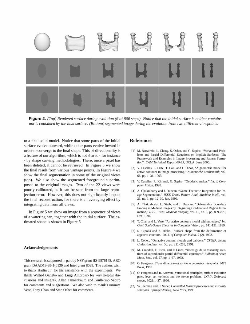
Figure 2. (Top) Rendered surface during evolution (6 of 800 steps). Notice that the initial surface is neither containsnor is contained by the final surface. (Bottom) segmented image during the evolution from two different viewpoints.

to a final solid model. Notice that some parts of the initialsurface evolve outward, while other parts evolve inward inorder to converge to the final shape. This bi-directionality isa feature of our algorithm, which is not shared - for instance- by shape carving methodologies. There, once a pixel hasbeen deleted, it cannot be retrieved. In Figure 3 we showthe final result from various vantage points. In Figure 4 weshow the final segmentation in some of the original views(top). We also show the segmented foreground superim-posed to the original images. Two of the 22 views werepoorly calibrated, as it can be seen from the large repro-jection error. However, this does not significantly impactthe final reconstruction, for there is an averaging effect byintegrating data from all views.

In Figure 5 we show an image from a sequence of viewsof a watering can, together with the initial surface. The es-timated shape is shown in Figure 6

Acknowledgements

This research is supported in part by NSF grant IIS-9876145, AROgrant DAAD19-99-1-0139 and Intel grant 8029. The authors wishto thank Hailin Jin for his assistance with the experiments. Wethank Wilfrid Gangbo and Luigi Ambrosio for very helpful dis-cussions and insights, Allen Tannenbaum and Guillermo Sapirofor comments and suggestions. We also wish to thank LuminitaVese, Tony Chan and Stan Osher for comments.

References

[1] M. Bertalmio, L. Cheng, S. Osher, and G. Sapiro, “Variational Prob-lems and Partial Differential Equations on Implicit Surfaces: TheFramework and Examples in Image Processing and Pattern Forma-tion”. CAM Technical Report 00-23, UCLA, June 2000.

[2] V. Caselles, F. Catte, T. Coll, and F. Dibos, “A geometric model foractive contours in image processing,” Numerische Mathematik, vol.66, pp. 1–31, 1993.

[3] V. Caselles, R. Kimmel, G. Sapiro, “Geodesic snakes,” Int. J. Com-puter Vision, 1998.

[4] A. Chakraborty and J. Duncan, “Game-Theoretic Integration for Im-age Segmentation,” IEEE Trans. Pattern Anal. Machine Intell., vol.21, no. 1, pp. 12–30, Jan. 1999.

[5] A. Chakraborty, L. Staib, and J. Duncan, “Deformable BoundaryFinding in Medical Images by Integrating Gradient and Region Infor-mation,” IEEE Trans. Medical Imaging, vol. 15, no. 6, pp. 859–870,Dec. 1996.

[6] T. Chan and L. Vese, “An active contours model without edges,” Int.Conf. Scale-Space Theories in Computer Vision, pp. 141-151, 1999.

[7] R. Cipolla and A. Blake. Surface shape from the deformation ofapparent contours. Int. J. of Computer Vision, 9 (2), 1992.

[8] L. Cohen, “On active contour models and balloons,” CVGIP: ImageUnderstanding, vol. 53, pp. 211–218, 1991.

[9] M. Crandall, H. Ishii, and P. Lions, “Users guide to viscosity solu-tions of second order partial differential equations,” Bulletin of Amer.Math. Soc., vol. 27, pp. 1–67, 1992.

[10] O. Faugeras. Three dimensional vision, a geometric viewpoint. MITPress, 1993.

[11] O. Faugeras and R. Keriven. Variational principles, surface evolutionpdes, level set methods and the stereo problem. INRIA Technicalreport, 3021:1–37, 1996.

[12] W. Fleming and H. Soner, Controlled Markov processes and viscositysolutions. Springer-Verlag, New York, 1993.

Figure 4. (Top) Image segmentation for the salt and pepper sequence. (Bottom) Segmented foreground superimposedto the original sequence. The calibration in two of the 22 images was inaccurate (one of which is shown above; thefourth image from the left). However, the effect is mitigated by the global integration, and the overall shape is onlymarginally affected by the calibration errors.

Figure 7. Rendered surface during evolution for the watering can.

[13] G. Gimelfarb and R. Haralick, “Terrain reconstruction from multipleviews,” in PRoc. 7th Intl. Conf. on Computer Analysis of Images andPatterns, pp. 695-701, 1997.

[14] B. Horn and M. Brooks (eds.). Shape from Shading. MIT Press,1989.

[15] M. Kass, A. Witkin, and D. Terzopoulos, “Snakes: active contourmodels,” Int. Journal of Computer Vision, vol. 1, pp. 321–331, 1987.

[16] S. Kichenassamy, A. Kumar, P. Olver, A. Tannenbaum, and A. Yezzi,“Conformal Curvature Flows: From Phase Transitions to Active Vi-sion,” Arch. Rational Mech. Anal., vol. 134, pp. 275–301, 1996.

[17] K. Kutulakos and S. Seitz. A theory of shape by space carving. InProc. of the Intl. Conf. on Comp. Vision, 1998.

[18] Y. Leclerc, “Constructing stable descriptions for image partitioning,”Int. J. Computer Vision, vol. 3, pp. 73–102, 1989.

[19] R. J. LeVeque, Numerical Methods for Conservation Laws,Birkhauser, Boston, 1992.

[20] P. L. Lions, Generalized Solutions of Hamilton-Jacobi Equations,Pitman Publishing, Boston, 1982.

[21] R. Malladi, J. Sethian, and B. Vemuri, “Shape modeling with frontpropagation: a level set approach,” IEEE Trans. Pattern Anal. Ma-chine Intell., vol. 17, pp. 158–175, 1995.

[22] D. Mumford and J. Shah. Optimal approximations by piecewisesmooth functions and associated variational problems. Comm. onPure and Applied Mathematics, 42:577–685, 1989.

[23] D. Mumford and J. Shah, ”Boundary detection by minimizing func-tionals,” Proceedings of IEEE Conference on Computer Vision andPattern Recognition, San Francisco, 1985.

[24] S. Osher, “Riemann solvers, the entropy condition, and differenceapproximations,” SIAM J. Numer. Anal., vol. 21, pp. 217–235, 1984.

[25] S. Osher and J. Sethian. Fronts propagating with curvature-dependent speed: algorithms based on Hamilton-Jacobi equations.J. of Comp. Physics, 79:12–49, 1988.

[26] N. Paragios and R. Deriche, “Geodesic Active Regions for Super-vised Texture Segmentation,” Proceedings of ICCV, Sept. 1999,Corfu, Greece.

[27] N. Paragios and R. Deriche, “Coupled Geodesic Active Regions forImage Segmentation: a level set approach,” Proceedings of ECCV,June 2000, Dublin, Ireland.

[28] R. Ronfard, “Region-Based Strategies for Active Contour Models,”Int. J. Computer Vision, vol. 13, no. 2, pp. 229–251, 1994.

[29] R. Rosenholtz and J. Malik. A differential method for comput-ing local shape-from-texture for planar and curved surfaces. UCB-CSD 93-775, Computer Science Division, University of California atBerkeley, 1993.

[30] C. Samson, L. Blanc-Feraud, G. Aubert, and J. Zerubia. “A Level SetMethod for Image Classification,” Int. Conf. Scale-Space Theories inComputer Vision, pp. 306-317, 1999.

[31] J. Sethian, Level Set Methods: Evolving Interfaces in Geometry,Fluid Mechanics, Computer Vision, and Material Science, Cam-bridge University Press, 1996.

[32] K. Siddiqi, Y. Lauziere, A. Tannenbaum, and S. Zucker, “Area andlength minimizing flows for segmentation,” IEEE Trans. Image Pro-cessing, vol. 7, pp. 433–444, 1998.

[33] D. Snow, P. Viola and R. Zabih, “Exact voxel occupancy with graphcuts,” Proc. of the Intl. Conf. on Comp. Vis. and Patt. Recog., 2000

Figure 3. Final estimated surface shown from sev-eral viewpoints. Notice that the bottoms of the saltand pepper shakers are flat, even though no data wasavailable. This is due to the geometric prior, which inthe absence of data results in a minimal surface beingcomputed.

[34] H. Tek and B. Kimia, “Image segmentation by reaction diffusionbubbles,” Proc. Int. Conf. Computer Vision, pp. 156–162, 1995.

[35] D. Terzopoulos and A. Witkin, “Constraints on deformable models:recovering shape and non-rigid motion,” Artificial Intelligence, vol.36, pp. 91–123, 1988.

[36] A. Yezzi, A. Tsai, and A. Willsky, “A Statistical Approach to ImageSegmentation for Bimodal and Trimodal Imagery,” Proceedings ofICCV, September, 1999.

[37] S. Zhu and A. Yuille, “Region Competition: Unifying snakes, Re-gion Growing, and Bayes/MDL for Multiband Image Segmentation,”IEEE Transactions on Pattern Analysis and Machine Intelligence,vol. 18, no. 9, pp. 884–900, Sep. 1996.

Figure 5. The “watering can” sequence and the ini-tial surface. Notice that the initial surface is not sim-ply connected and neither contains nor is containedby the final surface. In order to capture a hole it isnecessary that it is intersected by the initial surface.One way to guarantee this is to start with a number ofsmall surfaces.

Figure 6. Final estimated shape for the watering can.The two initial surfaces, as seen in Figure 5, havemerged. Although no ground truth is available forthese sequences, it is evident that the topology andgeometry of the watering can has been correctly cap-tured.