A&A 575, A63 (2015)DOI: 10.1051/0004-6361/201424929c© ESO 2015

Astronomy&

Astrophysics

Steps towards a high precision solar rotation profile: Resultsfrom SDO/AIA coronal bright point data

D. Sudar1, I. Skokic2, R. Brajša1, and S. H. Saar3

1 Hvar Observatory, Faculty of Geodesy, University of Zagreb, Kaciceva 26, 10000 Zagreb, Croatiae-mail: davor.sudar@gmail.com

2 Cybrotech Ltd, Bohinjska 11, 10000 Zagreb, Croatia3 Harvard-Smithsonian Center for Astrophysics, 60 Garden Street, Cambridge, MA 02138, USA

Received 5 September 2014 / Accepted 23 December 2014

ABSTRACT

Context. Coronal bright points (CBP) are ubiquitous small brightenings in the solar corona associated with small magnetic bipoles.Aims. We derive the solar differential rotation profile by tracing the motions of CBPs detected by the Atmospheric Imaging Assembly(AIA) instrument aboard the Solar Dynamics Observatory (SDO). We also investigate problems related to the detection of CBPsresulting from instrument and detection algorithm limitations.Methods. To determine the positions and identification of CBPs we used a segmentation algorithm. A linear fit of their centralmeridian distance and latitude vs time was used to derive velocities.Results. We obtained 906 velocity measurements in a time interval of only 2 days. The differential rotation profile can be expressedas ωrot = (14.◦47 ± 0.◦10 + (0.◦6 ± 1.◦0) sin2(b) + (−4.◦7 ± 1.◦7) sin4(b)) d−1. Our result is in agreement with other work and it comes withreasonable errors in spite of the very short time interval used. This was made possible by the higher sensitivity and resolution of theAIA instrument compared to similar equipment as well as high cadence. The segmentation algorithm also played a crucial role bydetecting so many CBPs, which reduced the errors to a reasonable level.Conclusions. Data and methods presented in this paper show a great potential for obtaining very accurate velocity profiles, bothfor rotation and meridional motion and, consequently, Reynolds stresses. The amount of CBP data that could be obtained from thisinstrument should also provide a great opportunity to study changes of velocity patterns with a temporal resolution of only a fewmonths. Other possibilities are studies of evolution of CBPs and proper motions of magnetic elements on the Sun.

Key words. Sun: rotation – Sun: corona – Sun: activity

1. Introduction

We present a new solar rotation profile obtained by tracingthe motions of coronal bright points (CBPs) observed by theAtmospheric Imaging Assembly (AIA) instrument on boardthe Solar Dynamics Observatory (SDO) satellite (Lemen et al.2012).

The most frequently used and oldest tracers of the solar dif-ferential rotation profile are sunspots (Newton & Nunn 1951;Howard et al. 1984; Balthasar et al. 1986b; Brajša et al. 2002a).One of the advantages of using sunspots is very long time cov-erage. On the other hand, there are numerous disadvantages:sunspots have complex and evolving structure, their distribu-tion in latitude is highly non-uniform, and they do not extendto higher solar latitudes. The number of sunspots is also highlyvariable during the solar cycle which makes measurements ofsolar differential rotation profiles almost impossible during solarminimum.

Coronal bright points are more uniformly distributed in lati-tude and are numerous in all phases of the solar cycle. They alsoextend over all solar latitudes. They have been used as tracersof solar rotation since the beginning of the space age (Dupree &Henze 1972). In recent years there have been numerous studiesinvestigating solar differential rotation by using CBPs as tracers.Kariyappa (2008), Hara (2009) used Yohkoh/SXT data, whileBrajša et al. (2001, 2002b, 2004), Vršnak et al. (2003), Wöhlet al. (2010) used SOHO/EIT observations in 28.4 nm channel,and Karachik et al. (2006) used 19.4 nm SOHO/EIT channel.

Kariyappa (2008) also used Hinode/XRT full-disk images todetermine the solar rotation profile.

Other tracers are used as well, for example magnetic fields(Wilcox & Howard 1970; Snodgrass 1983; Komm et al. 1993)and Hα filaments (Brajša et al. 1991). Apart from tracers,Doppler measurements can also be used (Howard & Harvey1970; Ulrich et al. 1988; Snodgrass & Ulrich 1990).

Helioseismic measurements also show differential rotationbelow the photosphere all the way down to the bottom of the con-vective zone (Kosovichev et al. 1997; Schou et al. 1998). Furtherdown, the rotation profile becomes uniform for all latitudes (seee.g. Howe 2009).

For further details about solar rotation, its importance for so-lar dynamo models, and a comparison of rotation measurementsbetween different sources, see the reviews by Schröter (1985),Howard (1984), Beck (2000), Ossendrijver (2003), Rüdiger &Hollerbach (2004), Stix (2004), Howe (2009) and Rozelot &Neiner (2009).

In this work we use CBP data obtained by SDO/AIA overonly two days to assess the quality of the data, identify sources oferrors and calculate the solar differential rotation profile. We willalso investigate the possibility of using CBP data from SDO/AIAfor further studies of other related phenomena (meridional flow,rotation velocity residuals, and Reynolds stress).

Coronal bright point data from SDO/AIA have also been inother works. Lorenc et al. (2012) discussed rotation of the so-lar corona based on 69 structures from 674 images detected inthe 9.4 nm channel using an interactive method of detection.

Article published by EDP Sciences A63, page 1 of 6

A&A 575, A63 (2015)

Dorotovic et al. (2014) presented a hybrid algorithm for detec-tion and tracking of CBPs. McIntosh et al. (2014b) used detec-tion algorithm presented in their previous paper (McIntosh &Gurman 2005) to identify CBPs in the SDO/AIA 19.4 nm chan-nel and correlate their properties with those of giant convectivecells. Using more SDO/AIA data and extending analysis back toSOHO era, McIntosh et al. (2014a) concluded that CBPs almostexclusively form around the vertices of giant convective cells.

2. Data and reduction methods

We used data from the AIA instrument on board the SDO satel-lite (Lemen et al. 2012). The spatial resolution of the in-strument is ≈0.6′′/pixel. For comparison, SOHO/EIT reso-lution is 2.629′′/pixel, while Hinode/XRT has a resolutionof 1.032′′/pixel.

To obtain positional information for the CBPs, we employeda segmentation algorithm which uses the 19.3 nm AIA channeldata to search for localized, small intensity enhancements in theEUV compared to a smoothed background intensity. More de-tails about the detection algorithm, which is similar to the algo-rithm by McIntosh & Gurman (2005), can be found in Martenset al. (2012).

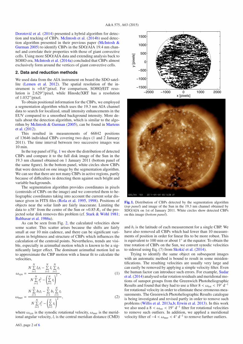
This resulted in measurements of 66842 positionsof 13646 individual CBPs covering two days (1 and 2 January2011). The time interval between two successive images was10 min.

In the top panel of Fig. 1 we show the distribution of detectedCBPs and compare it to the full disk image of the Sun in the19.3 nm channel obtained on 1 January 2011 (bottom panel ofthe same figure). In the bottom panel, white circles show CBPsthat were detected on one image by the segmentation algorithm.We can see that there are not many CBPs in active regions, partlybecause of difficulties in detecting them against such bright andvariable backgrounds.

The segmentation algorithm provides coordinates in pixels(centroids of CBPs on the image) and we converted them to he-liographic coordinates taking into account the current solar dis-tance given in FITS files (Roša et al. 1995, 1998). Positions ofobjects near the solar limb are fairly inaccurate. Limiting thedata to ±58◦ from the centre of the Sun or ≈0.85 R� of the pro-jected solar disk removes this problem (cf. Stark & Wöhl 1981;Balthasar et al. 1986a).

As can be seen from Fig. 2, the calculated velocities showsome scatter. This scatter arises because the shifts are fairlysmall at our 10 min cadence, and there can be significant vari-ations in brightness and structure of CBPs which influences thecalculation of the centroid points. Nevertheless, trends are visi-ble, especially in azimuthal motion which is known to be a sig-nificantly larger effect. The dominant azimuthal motion led usto approximate the CBP motion with a linear fit to calculate thevelocities,

ωsyn =

NN∑

i=1liti −

N∑i=1

liN∑

i=1ti

NN∑

i=1t2i −

(N∑

i=1ti

)2, (1)

ωmer =

NN∑

i=1biti −

N∑i=1

bi

N∑i=1

ti

NN∑

i=1t2i −

(N∑

i=1ti

)2, (2)

where ωsyn is the synodic rotational velocity, ωmer is the merid-ional angular velocity, li is the central meridian distance (CMD)

−2000 −1000 0 1000 2000−1500

−1000

−500

0

500

1000

1500

x [pixels]

y [p

ixel

s]

Fig. 1. Distribution of CBPs detected by the segmentation algorithm(top panel) and image of the Sun in the 19.3 nm channel obtained bySDO/AIA on 1st of January 2011. White circles show detected CBPson this image (bottom panel).

and bi is the latitude of each measurement for a single CBP. Wehave also removed all CBPs which had fewer than 10 measure-ments of position in order for linear fits to be more robust. Thisis equivalent to 100 min or about 1◦ at the equator. To obtain thetrue rotation of CBPs on the Sun, we convert synodic velocitiesto sidereal using Eq. (7) from Skokic et al. (2014).

Trying to identify the same object on subsequent imageswith an automatic method is bound to result in some misiden-tifications. The resulting velocities are usually very large andcan easily be removed by applying a simple velocity filter. Eventhe human factor can introduce such errors. For example, Sudaret al. (2014) analysed solar rotation residuals and meridional mo-tions of sunspot groups from the Greenwich PhotoheliographicResults and found that they had to use a filter 8 < ωrot < 19◦ d−1

for rotational velocity in order to eliminate these erroneous mea-surements. The Greenwich Photoheliographic Results catalogueis being investigated and revised partly in order to remove suchproblems (Willis et al. 2013a,b; Erwin et al. 2013). In this workwe also used a 8 < ωrot < 19◦ d−1 filter for rotational velocitiesto remove such outliers. In addition, we applied a meridionalvelocity filter of −4 < ωmer < 4◦ d−1 to remove further outliers.

A63, page 2 of 6

D. Sudar et al.: Steps towards a high precision solar rotation profile: Results from SDO/AIA coronal bright point data

-82.3

-82.2

-82.1

-82.0

-81.9

-81.8

0.00 0.02 0.04 0.06 0.08 0.10 0.12 0.14 0.16

b [d

eg]

t [days]

21.0

21.5

22.0

22.5

23.0

23.5

24.0

24.5

25.0

0.00 0.02 0.04 0.06 0.08 0.10 0.12 0.14 0.16

CM

D [d

eg]

t [days]

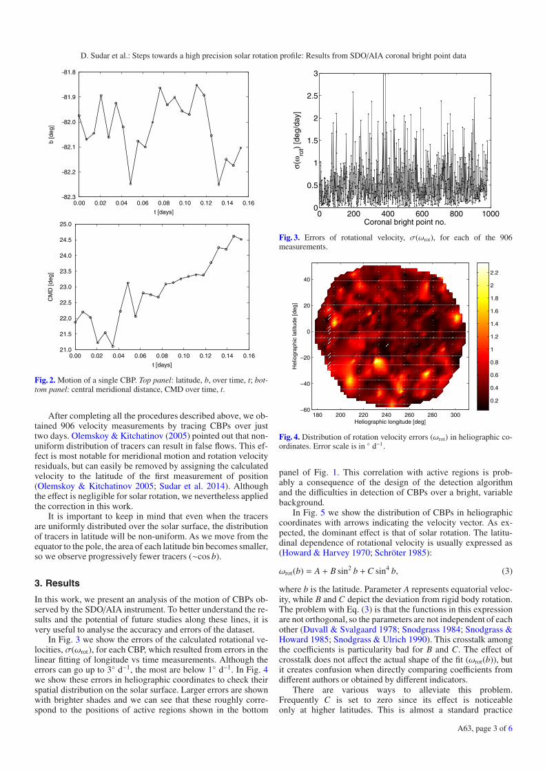
Fig. 2. Motion of a single CBP. Top panel: latitude, b, over time, t; bot-tom panel: central meridional distance, CMD over time, t.

After completing all the procedures described above, we ob-tained 906 velocity measurements by tracing CBPs over justtwo days. Olemskoy & Kitchatinov (2005) pointed out that non-uniform distribution of tracers can result in false flows. This ef-fect is most notable for meridional motion and rotation velocityresiduals, but can easily be removed by assigning the calculatedvelocity to the latitude of the first measurement of position(Olemskoy & Kitchatinov 2005; Sudar et al. 2014). Althoughthe effect is negligible for solar rotation, we nevertheless appliedthe correction in this work.

It is important to keep in mind that even when the tracersare uniformly distributed over the solar surface, the distributionof tracers in latitude will be non-uniform. As we move from theequator to the pole, the area of each latitude bin becomes smaller,so we observe progressively fewer tracers (∼cos b).

3. Results

In this work, we present an analysis of the motion of CBPs ob-served by the SDO/AIA instrument. To better understand the re-sults and the potential of future studies along these lines, it isvery useful to analyse the accuracy and errors of the dataset.

In Fig. 3 we show the errors of the calculated rotational ve-locities, σ(ωrot), for each CBP, which resulted from errors in thelinear fitting of longitude vs time measurements. Although theerrors can go up to 3◦ d−1, the most are below 1◦ d−1. In Fig. 4we show these errors in heliographic coordinates to check theirspatial distribution on the solar surface. Larger errors are shownwith brighter shades and we can see that these roughly corre-spond to the positions of active regions shown in the bottom

0 200 400 600 800 10000

0.5

1

1.5

2

2.5

3

Coronal bright point no.

σ(ω

rot)

[deg

/day

]

Fig. 3. Errors of rotational velocity, σ(ωrot), for each of the 906measurements.

180 200 220 240 260 280 300−60

−40

−20

0

20

40

Heliographic longitude [deg]

Hel

iogr

aphi

c la

titud

e [d

eg]

0.2

0.4

0.6

0.8

1

1.2

1.4

1.6

1.8

2

2.2

Fig. 4. Distribution of rotation velocity errors (ωrot) in heliographic co-ordinates. Error scale is in ◦ d−1.

panel of Fig. 1. This correlation with active regions is prob-ably a consequence of the design of the detection algorithmand the difficulties in detection of CBPs over a bright, variablebackground.

In Fig. 5 we show the distribution of CBPs in heliographiccoordinates with arrows indicating the velocity vector. As ex-pected, the dominant effect is that of solar rotation. The latitu-dinal dependence of rotational velocity is usually expressed as(Howard & Harvey 1970; Schröter 1985):

ωrot(b) = A + B sin2 b +C sin4 b, (3)

where b is the latitude. Parameter A represents equatorial veloc-ity, while B and C depict the deviation from rigid body rotation.The problem with Eq. (3) is that the functions in this expressionare not orthogonal, so the parameters are not independent of eachother (Duvall & Svalgaard 1978; Snodgrass 1984; Snodgrass &Howard 1985; Snodgrass & Ulrich 1990). This crosstalk amongthe coefficients is particularity bad for B and C. The effect ofcrosstalk does not affect the actual shape of the fit (ωrot(b)), butit creates confusion when directly comparing coefficients fromdifferent authors or obtained by different indicators.

There are various ways to alleviate this problem.Frequently C is set to zero since its effect is noticeableonly at higher latitudes. This is almost a standard practice

A63, page 3 of 6

A&A 575, A63 (2015)

160 180 200 220 240 260 280 300 320 340−80

−60

−40

−20

0

20

40

60

Heliographic longitude [deg]

Hel

iogr

aphi

c la

titud

e [d

eg]

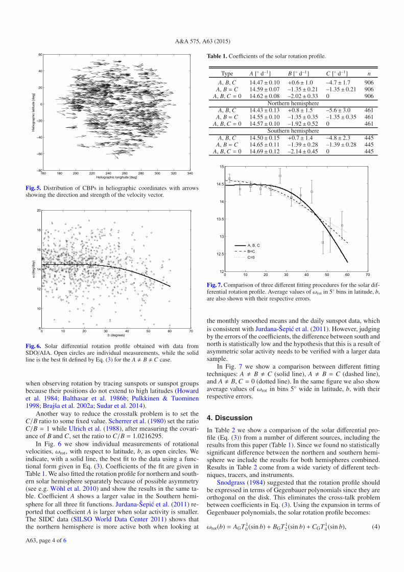
Fig. 5. Distribution of CBPs in heliographic coordinates with arrowsshowing the direction and strength of the velocity vector.

0 10 20 30 40 50 60 708

10

12

14

16

18

20

ω (

deg/

day)

b (degrees)

Fig. 6. Solar differential rotation profile obtained with data fromSDO/AIA. Open circles are individual measurements, while the solidline is the best fit defined by Eq. (3) for the A � B � C case.

when observing rotation by tracing sunspots or sunspot groupsbecause their positions do not extend to high latitudes (Howardet al. 1984; Balthasar et al. 1986b; Pulkkinen & Tuominen1998; Brajša et al. 2002a; Sudar et al. 2014).

Another way to reduce the crosstalk problem is to set theC/B ratio to some fixed value. Scherrer et al. (1980) set the ratioC/B = 1 while Ulrich et al. (1988), after measuring the covari-ance of B and C, set the ratio to C/B = 1.0216295.

In Fig. 6 we show individual measurements of rotationalvelocities, ωrot, with respect to latitude, b, as open circles. Weindicate, with a solid line, the best fit to the data using a func-tional form given in Eq. (3). Coefficients of the fit are given inTable 1. We also fitted the rotation profile for northern and south-ern solar hemisphere separately because of possible asymmetry(see e.g. Wöhl et al. 2010) and show the results in the same ta-ble. Coefficient A shows a larger value in the Southern hemi-sphere for all three fit functions. Jurdana-Šepic et al. (2011) re-ported that coefficient A is larger when solar activity is smaller.The SIDC data (SILSO World Data Center 2011) shows thatthe northern hemisphere is more active both when looking at

Table 1. Coefficients of the solar rotation profile.

Type A [◦ d−1] B [◦ d−1] C [◦ d−1] n

A, B, C 14.47± 0.10 +0.6± 1.0 –4.7± 1.7 906A, B = C 14.59± 0.07 –1.35± 0.21 –1.35± 0.21 906

A, B, C = 0 14.62± 0.08 –2.02± 0.33 0 906Northern hemisphere

A, B, C 14.43± 0.13 +0.8± 1.5 –5.6± 3.0 461A, B = C 14.55± 0.10 –1.35± 0.35 –1.35± 0.35 461

A, B, C = 0 14.57± 0.10 –1.92± 0.52 0 461Southern hemisphere

A, B, C 14.50± 0.15 +0.7± 1.4 –4.8± 2.3 445A, B = C 14.65± 0.11 –1.39± 0.28 –1.39± 0.28 445

A, B, C = 0 14.69± 0.12 –2.14± 0.45 0 445

0 10 20 30 40 50 60 7012

12.5

13

13.5

14

14.5

15

A, B, CB=CC=0

Fig. 7. Comparison of three different fitting procedures for the solar dif-ferential rotation profile. Average values of ωrot in 5◦ bins in latitude, b,are also shown with their respective errors.

the monthly smoothed means and the daily sunspot data, whichis consistent with Jurdana-Šepic et al. (2011). However, judgingby the errors of the coefficients, the difference between south andnorth is statistically low and the hypothesis that this is a result ofasymmetric solar activity needs to be verified with a larger datasample.

In Fig. 7 we show a comparison between different fittingtechniques: A � B � C (solid line), A � B = C (dashed line),and A � B, C = 0 (dotted line). In the same figure we also showaverage values of ωrot in bins 5◦ wide in latitude, b, with theirrespective errors.

4. Discussion

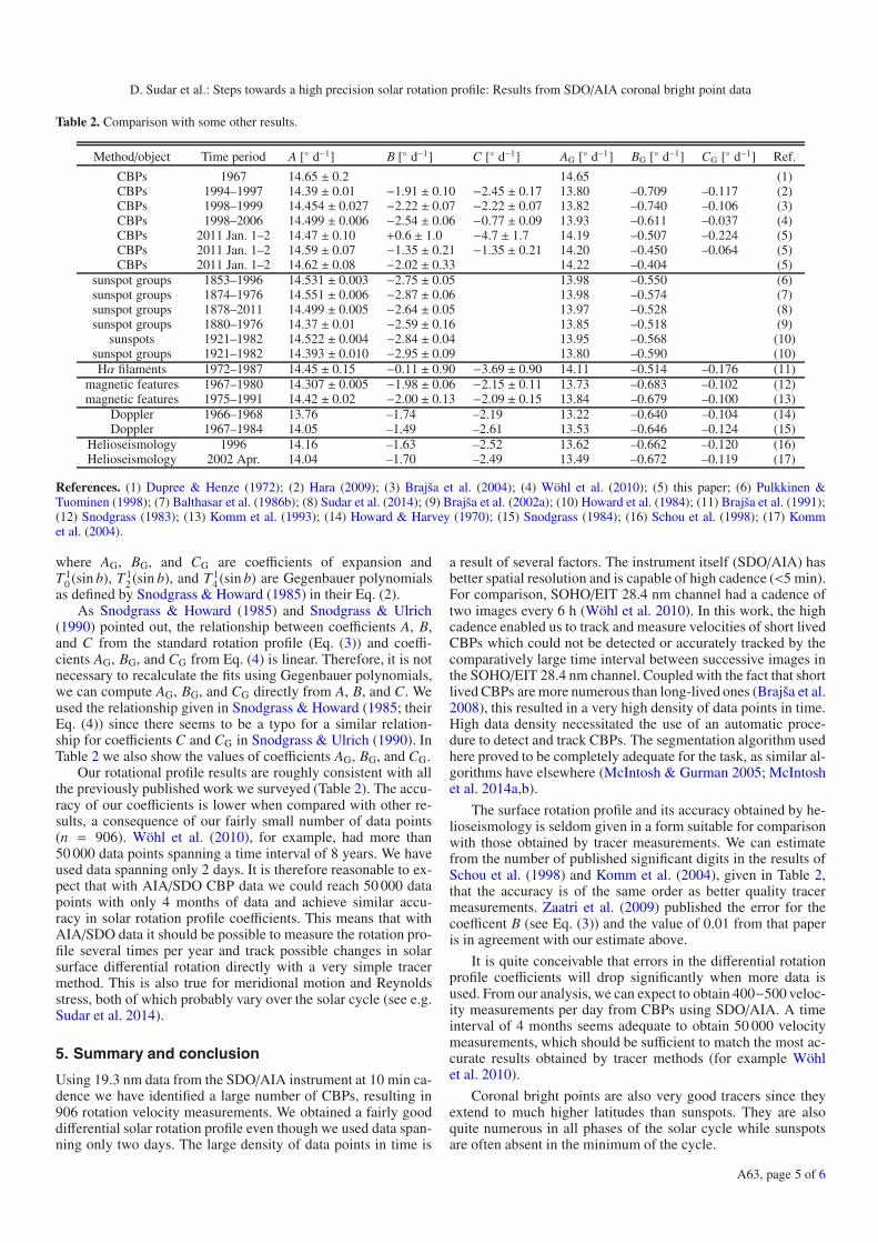
In Table 2 we show a comparison of the solar differential pro-file (Eq. (3)) from a number of different sources, including theresults from this paper (Table 1). Since we found no statisticallysignificant difference between the northern and southern hemi-sphere we include the results for both hemispheres combined.Results in Table 2 come from a wide variety of different tech-niques, tracers, and instruments.

Snodgrass (1984) suggested that the rotation profile shouldbe expressed in terms of Gegenbauer polynomials since they areorthogonal on the disk. This eliminates the cross-talk problembetween coefficients in Eq. (3). Using the expansion in terms ofGegenbauer polynomials, the solar rotation profile becomes:

ωrot(b) = AGT 10 (sin b) + BGT 1

2 (sin b) +CGT 14 (sin b), (4)

A63, page 4 of 6

D. Sudar et al.: Steps towards a high precision solar rotation profile: Results from SDO/AIA coronal bright point data

Table 2. Comparison with some other results.

Method/object Time period A [◦ d−1] B [◦ d−1] C [◦ d−1] AG [◦ d−1] BG [◦ d−1] CG [◦ d−1] Ref.

CBPs 1967 14.65 ± 0.2 14.65 (1)CBPs 1994–1997 14.39 ± 0.01 −1.91 ± 0.10 −2.45 ± 0.17 13.80 –0.709 –0.117 (2)CBPs 1998–1999 14.454 ± 0.027 −2.22 ± 0.07 −2.22 ± 0.07 13.82 –0.740 –0.106 (3)CBPs 1998–2006 14.499 ± 0.006 −2.54 ± 0.06 −0.77 ± 0.09 13.93 –0.611 –0.037 (4)CBPs 2011 Jan. 1–2 14.47 ± 0.10 +0.6 ± 1.0 −4.7 ± 1.7 14.19 –0.507 –0.224 (5)CBPs 2011 Jan. 1–2 14.59 ± 0.07 −1.35 ± 0.21 −1.35 ± 0.21 14.20 –0.450 –0.064 (5)CBPs 2011 Jan. 1–2 14.62 ± 0.08 −2.02 ± 0.33 14.22 –0.404 (5)

sunspot groups 1853–1996 14.531 ± 0.003 −2.75 ± 0.05 13.98 –0.550 (6)sunspot groups 1874–1976 14.551 ± 0.006 −2.87 ± 0.06 13.98 –0.574 (7)sunspot groups 1878–2011 14.499 ± 0.005 −2.64 ± 0.05 13.97 –0.528 (8)sunspot groups 1880–1976 14.37 ± 0.01 −2.59 ± 0.16 13.85 –0.518 (9)

sunspots 1921–1982 14.522 ± 0.004 −2.84 ± 0.04 13.95 –0.568 (10)sunspot groups 1921–1982 14.393 ± 0.010 −2.95 ± 0.09 13.80 –0.590 (10)Hα filaments 1972–1987 14.45 ± 0.15 −0.11 ± 0.90 −3.69 ± 0.90 14.11 –0.514 –0.176 (11)

magnetic features 1967–1980 14.307 ± 0.005 −1.98 ± 0.06 −2.15 ± 0.11 13.73 –0.683 –0.102 (12)magnetic features 1975–1991 14.42 ± 0.02 −2.00 ± 0.13 −2.09 ± 0.15 13.84 –0.679 –0.100 (13)

Doppler 1966–1968 13.76 –1.74 –2.19 13.22 –0.640 –0.104 (14)Doppler 1967–1984 14.05 –1.49 –2.61 13.53 –0.646 –0.124 (15)

Helioseismology 1996 14.16 –1.63 –2.52 13.62 –0.662 –0.120 (16)Helioseismology 2002 Apr. 14.04 –1.70 –2.49 13.49 –0.672 –0.119 (17)

References. (1) Dupree & Henze (1972); (2) Hara (2009); (3) Brajša et al. (2004); (4) Wöhl et al. (2010); (5) this paper; (6) Pulkkinen &Tuominen (1998); (7) Balthasar et al. (1986b); (8) Sudar et al. (2014); (9) Brajša et al. (2002a); (10) Howard et al. (1984); (11) Brajša et al. (1991);(12) Snodgrass (1983); (13) Komm et al. (1993); (14) Howard & Harvey (1970); (15) Snodgrass (1984); (16) Schou et al. (1998); (17) Kommet al. (2004).

where AG, BG, and CG are coefficients of expansion andT 1

0 (sin b), T 12 (sin b), and T 1

4 (sin b) are Gegenbauer polynomialsas defined by Snodgrass & Howard (1985) in their Eq. (2).

As Snodgrass & Howard (1985) and Snodgrass & Ulrich(1990) pointed out, the relationship between coefficients A, B,and C from the standard rotation profile (Eq. (3)) and coeffi-cients AG, BG, and CG from Eq. (4) is linear. Therefore, it is notnecessary to recalculate the fits using Gegenbauer polynomials,we can compute AG, BG, and CG directly from A, B, and C. Weused the relationship given in Snodgrass & Howard (1985; theirEq. (4)) since there seems to be a typo for a similar relation-ship for coefficients C and CG in Snodgrass & Ulrich (1990). InTable 2 we also show the values of coefficients AG, BG, and CG.

Our rotational profile results are roughly consistent with allthe previously published work we surveyed (Table 2). The accu-racy of our coefficients is lower when compared with other re-sults, a consequence of our fairly small number of data points(n = 906). Wöhl et al. (2010), for example, had more than50 000 data points spanning a time interval of 8 years. We haveused data spanning only 2 days. It is therefore reasonable to ex-pect that with AIA/SDO CBP data we could reach 50 000 datapoints with only 4 months of data and achieve similar accu-racy in solar rotation profile coefficients. This means that withAIA/SDO data it should be possible to measure the rotation pro-file several times per year and track possible changes in solarsurface differential rotation directly with a very simple tracermethod. This is also true for meridional motion and Reynoldsstress, both of which probably vary over the solar cycle (see e.g.Sudar et al. 2014).

5. Summary and conclusion

Using 19.3 nm data from the SDO/AIA instrument at 10 min ca-dence we have identified a large number of CBPs, resulting in906 rotation velocity measurements. We obtained a fairly gooddifferential solar rotation profile even though we used data span-ning only two days. The large density of data points in time is

a result of several factors. The instrument itself (SDO/AIA) hasbetter spatial resolution and is capable of high cadence (<5 min).For comparison, SOHO/EIT 28.4 nm channel had a cadence oftwo images every 6 h (Wöhl et al. 2010). In this work, the highcadence enabled us to track and measure velocities of short livedCBPs which could not be detected or accurately tracked by thecomparatively large time interval between successive images inthe SOHO/EIT 28.4 nm channel. Coupled with the fact that shortlived CBPs are more numerous than long-lived ones (Brajša et al.2008), this resulted in a very high density of data points in time.High data density necessitated the use of an automatic proce-dure to detect and track CBPs. The segmentation algorithm usedhere proved to be completely adequate for the task, as similar al-gorithms have elsewhere (McIntosh & Gurman 2005; McIntoshet al. 2014a,b).

The surface rotation profile and its accuracy obtained by he-lioseismology is seldom given in a form suitable for comparisonwith those obtained by tracer measurements. We can estimatefrom the number of published significant digits in the results ofSchou et al. (1998) and Komm et al. (2004), given in Table 2,that the accuracy is of the same order as better quality tracermeasurements. Zaatri et al. (2009) published the error for thecoefficent B (see Eq. (3)) and the value of 0.01 from that paperis in agreement with our estimate above.

It is quite conceivable that errors in the differential rotationprofile coefficients will drop significantly when more data isused. From our analysis, we can expect to obtain 400−500 veloc-ity measurements per day from CBPs using SDO/AIA. A timeinterval of 4 months seems adequate to obtain 50 000 velocitymeasurements, which should be sufficient to match the most ac-curate results obtained by tracer methods (for example Wöhlet al. 2010).

Coronal bright points are also very good tracers since theyextend to much higher latitudes than sunspots. They are alsoquite numerous in all phases of the solar cycle while sunspotsare often absent in the minimum of the cycle.

A63, page 5 of 6

A&A 575, A63 (2015)

This opens up an intriguing possibility of measuring the so-lar rotation profile almost from one month to the next over anentire cycle. Such studies could provide new insight into themechanisms responsible for solar rotation. We already knowthat meridional motion exhibits some changes during the courseof the solar cycle, and the same is probably true for Reynoldsstress. Sudar et al. (2014) found by averaging almost 150 yearsof sunspot data that meridional motion changes slightly over thesolar cycle and hinted that the Reynolds stresses are probablychanging too. Here we have found a small asymmetry in rota-tion profile for two solar hemispheres and suggested that thismight be related to different solar activity levels in the two hemi-spheres. This needs to be verified with a larger dataset, how-ever, as the difference in rotation profiles was of low statisticalsignificance.

The planned SDO mission duration of 5–10 years will covera large portion of the solar cycle which should result in an enor-mous amount of velocity data to assist in the understanding ofthe nature and variation of solar rotation profile. Having moredetailed temporal resolution and direct results (without the needto average many solar cycles) could prove to be very informative.

A time interval of 10 min between successive images alsooffers a good opportunity to study the evolution of CBPs and thepossible effect this might have on the detected surface velocityfields. For example, Vršnak et al. (2003) reported that longerlasting CBPs show different results than short-lived CBPs.

Based on the promising results here, we will use largerdatasets to further exploit the potential of SDO/AIA CBP datato determine meridional motions, rotation velocity residuals,Reynolds stresses, and proper motions in subsequent papers.

Acknowledgements. This work has received funding from the EuropeanCommission FP7 project eHEROES (284461, 2012–2015) and SOLARNETproject (312495, 2013-2017) which is an Integrated Infrastructure Initiative (I3)supported by FP7 Capacities Programme. It was also supported by the CroatianScience Foundation under the project 6212 Solar and Stellar Variability. SS wassupported by NASA Grant NNX09AB03G to the Smithsonian AstrophysicalObservatory and contract SP02H1701R from Lockheed-Martin to SAO. Wewould like to thank the SDO/AIA science teams for providing the observa-tions. We would also like to thank Veronique Delouille and Alexander Engellfor valuable help in the preparation of this work.

References

Balthasar, H., Lustig, G., Woehl, H., & Stark, D. 1986a, A&A, 160, 277Balthasar, H., Vázquez, M., & Wöhl, H. 1986b, A&A, 155, 87Beck, J. G. 2000, Sol. Phys., 191, 47Brajša, R., Vršnak, B., Ruždjak, V., Schroll, A., & Pohjolainen, S. 1991,

Sol. Phys., 133, 195Brajša, R., Wöhl, H., Vršnak, B., et al. 2001, A&A, 374, 309Brajša, R., Wöhl, H., Vršnak, B., et al. 2002a, Sol. Phys., 206, 229Brajša, R., Wöhl, H., Vršnak, B., et al. 2002b, A&A, 392, 329

Brajša, R., Wöhl, H., Vršnak, B., et al. 2004, A&A, 414, 707Brajša, R., Wöhl, H., Vršnak, B., et al. 2008, Central Europ. Astrophys. Bull.,

32, 165Dorotovic, I., Shahamatnia, E., Lorenc, M., et al. 2014, Sun and Geosphere,

9, 81Dupree, A. K., & Henze, Jr., W. 1972, Sol. Phys., 27, 271Duvall, Jr., T. L., & Svalgaard, L. 1978, Sol. Phys., 56, 463Erwin, E. H., Coffey, H. E., Denig, W. F., et al. 2013, Sol. Phys., 288, 157Hara, H. 2009, ApJ, 697, 980Howard, R. 1984, ARA&A, 22, 131Howard, R., & Harvey, J. 1970, Sol. Phys., 12, 23Howard, R., Gilman, P. I., & Gilman, P. A. 1984, ApJ, 283, 373Howe, R. 2009, Liv. Rev. Sol. Phys., 6, 1Jurdana-Šepic, R., Brajša, R., Wöhl, H., et al. 2011, A&A, 534, A17Karachik, N., Pevtsov, A. A., & Sattarov, I. 2006, ApJ, 642, 562Kariyappa, R. 2008, A&A, 488, 297Komm, R. W., Howard, R. F., & Harvey, J. W. 1993, Sol. Phys., 145, 1Komm, R., Corbard, T., Durney, B. R., et al. 2004, ApJ, 605, 554Kosovichev, A. G., Schou, J., Scherrer, P. H., et al. 1997, Sol. Phys., 170, 43Lemen, J. R., Title, A. M., Akin, D. J., et al. 2012, Sol. Phys., 275, 17Lorenc, M., Rybanský, M., & Dorotovic, I. 2012, Sol. Phys., 281, 611Martens, P. C. H., Attrill, G. D. R., Davey, A. R., et al. 2012, Sol. Phys., 275, 79McIntosh, S. W., & Gurman, J. B. 2005, Sol. Phys., 228, 285McIntosh, S. W., Wang, X., Leamon, R. J., et al. 2014a, ApJ, 792, 12McIntosh, S. W., Wang, X., Leamon, R. J., & Scherrer, P. H. 2014b, ApJ, 784,

L32Newton, H. W., & Nunn, M. L. 1951, MNRAS, 111, 413Olemskoy, S. V., & Kitchatinov, L. L. 2005, Astron. Lett., 31, 706Ossendrijver, M. 2003, A&ARv, 11, 287Pulkkinen, P., & Tuominen, I. 1998, A&A, 332, 755Roša, D., Vršnak, B., & Božic, H. 1995, Hvar Observatory Bulletin, 19, 23Roša, D., Vršnak, B., Božic, H., et al. 1998, Sol. Phys., 179, 237Rozelot, J.-P., & Neiner, C. 2009, The Rotation of Sun and Stars (Berlin:

Springer Verlag), Lect. Notes Phys., 765Rüdiger, G., & Hollerbach, R. 2004, The Magnetic Universe (Wiley

Interscience)Scherrer, P. H., Wilcox, J. M., & Svalgaard, L. 1980, ApJ, 241, 811Schou, J., Antia, H. M., Basu, S., et al. 1998, ApJ, 505, 390Schröter, E. H. 1985, Sol. Phys., 100, 141SILSO World Data Center 2011, International Sunspot Number Monthly

Bulletin and online catalogueSkokic, I., Brajša, R., Roša, D., Hržina, D., & Wöhl, H. 2014, Sol. Phys., 289,

1471Snodgrass, H. B. 1983, ApJ, 270, 288Snodgrass, H. B. 1984, Sol. Phys., 94, 13Snodgrass, H. B., & Howard, R. 1985, Sol. Phys., 95, 221Snodgrass, H. B., & Ulrich, R. K. 1990, ApJ, 351, 309Stark, D., & Wöhl, H. 1981, A&A, 93, 241Stix, M. 2004, The Sun: an introduction, 2nd edn., Astron. Astrophys. Libr.

(Berlin: Springer)Sudar, D., Skokic, I., Ruždjak, D., Brajša, R., & Wöhl, H. 2014, MNRAS, 439,

2377Ulrich, R. K., Boyden, J. E., Webster, L., Padilla, S. P., & Snodgrass, H. B. 1988,

Sol. Phys., 117, 291Vršnak, B., Brajša, R., Wöhl, H., et al. 2003, A&A, 404, 1117Wilcox, J. M., & Howard, R. 1970, Sol. Phys., 13, 251Willis, D. M., Coffey, H. E., Henwood, R., et al. 2013a, Sol. Phys., 288, 117Willis, D. M., Henwood, R., Wild, M. N., et al. 2013b, Sol. Phys., 288, 141Wöhl, H., Brajša, R., Hanslmeier, A., & Gissot, S. F. 2010, A&A, 520, A29Zaatri, A., Wöhl, H., Roth, M., Corbard, T., & Brajša, R. 2009, A&A, 504, 589

A63, page 6 of 6