Steel Structures Design Manual To AS 4100 First Edition Brian Kirke Senior Lecturer in Civil Engineering Griffith University

Iyad Hassan Al-Jamel

Managing DirectorADG Engineers Jordan

Copyright© Brian Kirke and Iyad Hassan Al-Jamel This book is copyright. Apart from any fair dealing for the purposes of private

study, research, criticism or review as permitted under the Copyright Act, no part

may be reproduced, stored in a retrieval system, or transmitted, in any form or by

any means electronic, mechanical, photocopying, recording or otherwise without

prior permission to the authors.

iii

CONTENTS_______________________________________________________

PREFACE viiiNOTATION x

1 INTRODUCTION: THE STRUCTURAL DESIGN PROCESS 1

1.1 Problem Formulation 1 1.2 Conceptual Design 1 1.3 Choice of Materials 3 1.4 Estimation of Loads 4 1.5 Structural Analysis 5 1.6 Member Sizing, Connections and Documentation 5 2 STEEL PROPERTIES 6

2.1 Introduction 6 2.2 Strength, Stiffness and Density 6 2.3 Ductility 6 2.3.1 Metallurgy and Transition Temperature 7 2.3.2 Stress Effects 7 2.3.3 Case Study: King’s St Bridge, Melbourne 8 2.4 Consistency 9 2.5 Corrosion 10 2.6 Fatigue Strength 11 2.7 Fire Resistance 12

2.8 References 13

3 LOAD ESTIMATION 14

3.1 Introduction 14 3.2 Estimating Dead Load (G) 14 3.2.1 Example: Concrete Slab on Columns 14 3.2.2 Concrete Slab on Steel Beams and Columns 16 3.2.3 Walls 17 3.2.4 Light Steel Construction 17 3.2.5 Roof Construction 18 3.2.6 Floor Construction 18 3.2.7 Sample Calculation of Dead Load for a Steel Roof 19 3.2.7.1 Dead Load on Purlins 20 3.2.7.2 Dead Load on Rafters 21 3.2.8 Dead Load due to a Timber Floor 22 3.2.9 Worked Examples on Dead Load Estimation 22 3.3 Estimating Live Load (Q) 24 3.3.1 Live Load Q on a Roof 24 3.3.2 Live Load Q on a Floor 24 3.3.3 Other Live Loads 24 3.3.4 Worked Examples of Live Load Estimation 25

iv Contents

3.4 Wind Load Estimation 26 3.4.1 Factors Influencing Wind Loads 26 3.4.2 Design Wind Speeds 28 3.4.3 Site Wind Speed Vsit,� 29 3.4.3.1 Regional Wind Speed VR 29 3.4.3.2 Wind Direction Multiplier Md 30 3.4.3.3 Terrain and Height Multiplier Mz,cat 30 3.4.3.4 Other Multipliers 30 3.4.4 Aerodynamic Shape Factor Cfig and Dynamic Response Factor Cdyn 33 3.4.5 Calculating External Pressures 33 3.4.6 Calculating Internal Pressures 38 3.4.7 Frictional Drag 39 3.4.8 Net Pressures 39 3.4.9 Exposed Structural Members 39 3.4.10 Worked Examples on Wind Load Estimation 40

3.5 Snow Loads 47 3.5.1 Example on Snow Load Estimation 47

3.6 Dynamic Loads and Resonance 48 3.6.1 Live Loads due to Vehicles in Car Parks 48 3.6.2 Crane, Hoist and Lift Loads 48 3.6.3 Unbalanced Rotating Machinery 48 3.6.4 Vortex Shedding 50 3.6.5 Worked Examples on Dynamic Loading 51 3.6.5.1 Acceleration Loads 51 3.6.5.2 Crane Loads 51 3.6.5.3 Unbalanced Machines 53 3.6.5.4 Vortex Shedding 54

3.7 Earthquake Loads 54 3.7.1 Basic Concepts 54 3.7.2 Design Procedure 55

3.7.3 Worked Examples on Earthquake Load Estimation 56 3.7.3.1 Earthquake Loading on a Tank Stand 56 3.7.3.1 Earthquake Loading on a Multi-Storey Building 56

3.8 Load Combinations 57 3.8.1 Application 57 3.8.2 Strength Design Load Combinations 57 3.8.3 Serviceability Design Load Combinations 58

3.9 References 59

4 METHODS OF STRUCTURAL ANALYSIS 60

4.1 Introduction 60 4.2 Methods of Determining Action Effects 60 4.3 Forms of Construction Assumed for Structural Analysis 61 4.4 Assumption for Analysis 61 4.5 Elastic Analysis 65 4.5.2 Moment Amplification 67 4.5.3 Moment Distribution 70 4.5.4 Frame Analysis Software 70

Contents v

4.5.5 Finite Element Analysis 714.6 Plastic Method of Structural Analysis 71 4.7 Member Buckling Analysis 73 4.8 Frame Buckling Analysis 77 4.9 References 79

5 DESIGN of TENSION MEMBERS 80

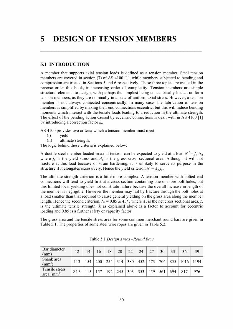
5.1 Introduction 80 5.2 Design of Tension Members to AS 4100 81 5.3 Worked Examples 82 5.3.1 Truss Member in Tension 82 5.3.2 Checking a Compound Tension Member with Staggered Holes 82 5.3.3 Checking a Threaded Rod with Turnbuckles 84 5.3.4 Designing a Single Angle Bracing 84 5.3.5 Designing a Steel Wire Rope Tie 85 5.4 References 85

6 DESIGN OF COMPRESSION MEMBERS 86

6.1 Introduction 86 6.2 Effective Lengths of Compression Members 91 6.3 Design of Compression Members to AS 4100 96 6.4 Worked Examples 98 6.4.1 Slender Bracing 98 6.4.2 Bracing Strut 99 6.4.3 Sizing an Intermediate Column in a Multi-Storey Building 99 6.4.4 Checking a Tee Section 101 6.4.5 Checking Two Angles Connected at Intervals 102 6.4.6 Checking Two Angles Connected Back to Back 103 6.4.7 Laced Compression Member 104 6.5 References 106

7 DESIGN OF FLEXURAL MEMBERS 107

7.1 Introduction 107 7.1.1 Beam Terminology 107 7.1.2 Compact, Non-Compact, and Slender-Element Sections 107 7.1.3 Lateral Torsional Buckling 108 7.2 Design of Flexural Members to AS 4100 109 7.2.1 Design for Bending Moment 109

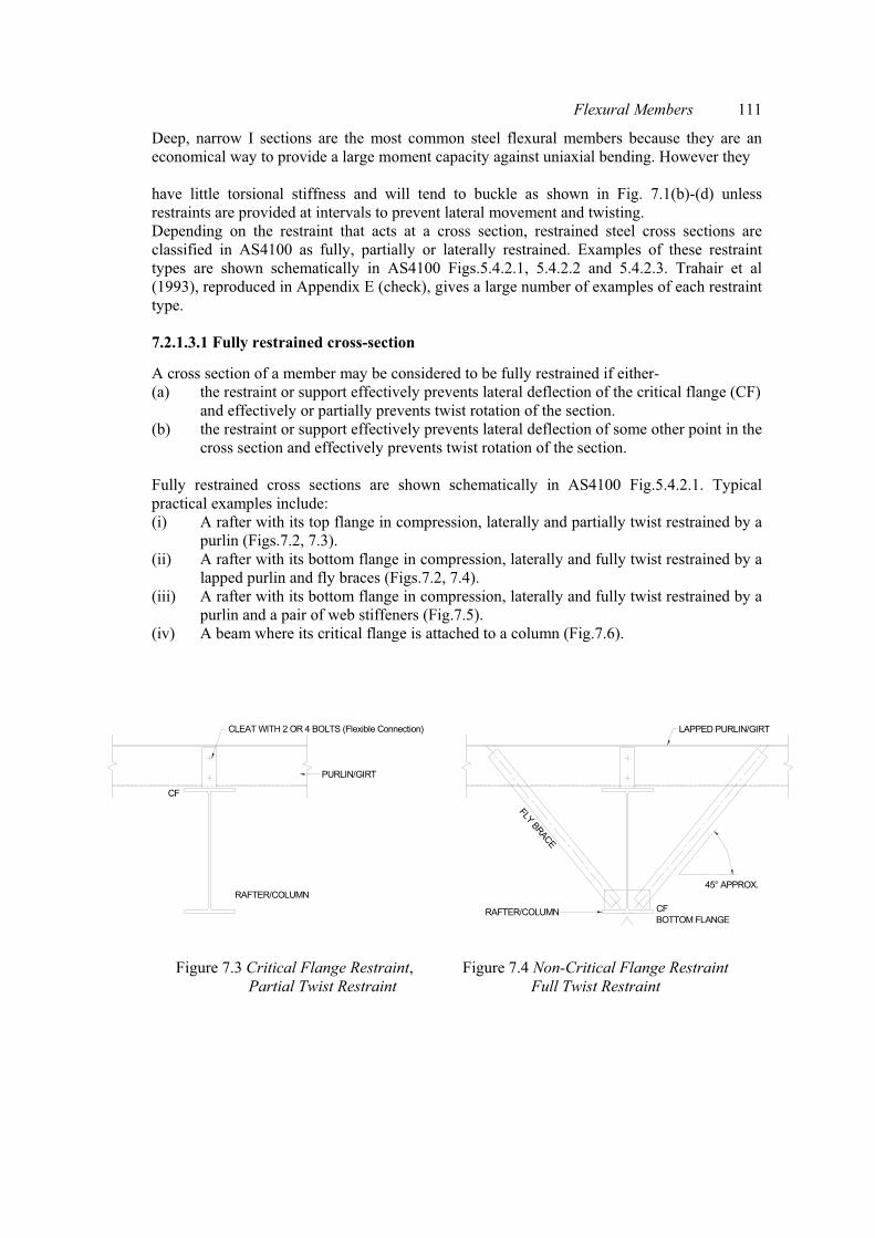
7.2.1.1 Lateral Buckling Behaviour of Unbraced Beams 109 7.2.1.2 Critical Flange 110

vi Contents

7.2.1.3 Restraints at a Cross Section 110 7.2.1.3.1 Fully Restrained Cross-Section 111 7.2.1.3.1 Partially Restrained Cross-Section 112 7.2.1.3.1 Laterally Restrained Cross-Section 113

7.2.1.4 Segments, Sub-Segments and Effective length 113 7.2.1.5 Member Moment Capacity of a Segment 114 7.2.1.6 Lateral Torsional Buckling Design Methodology 117

7.2.2 Design for Shear Force 117 7.3 Worked Examples 118 7.3.1 Moment Capacity of Steel Beam Supporting Concrete Slab 118 7.3.2 Moment Capacity of Simply Supported Rafter Under Uplift Load 118 7.3.3 Moment Capacity of Simply Supported Rafter Under Downward Load 120 7.3.4 Checking a Rigidly Connected Rafter Under Uplift 121 7.3.5 Designing a Rigidly Connected Rafter Under Uplift 123 7.3.6 Checking a Simply Supported Beam with Overhang 124 7.3.7 Checking a Tapered Web Beam 126 7.3.8 Bending in a Non-Principal Plane 127 7.3.9 Checking a flange stepped beam 128 7.3.10 Checking a tee section 129 7.3.11 Steel beam complete design check 131 7.3.12 Checking an I-section with unequal flanges 136 7.4 References 140

8 MEMBERS SUBJECT TO COMBINED ACTIONS 141

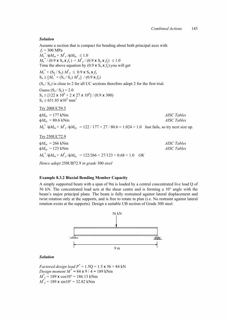
8.1 Introduction 141 8.2 Plastic Analysis and Plastic Design 142 8.3 Worked Examples 144 8.3.1 Biaxial Bending Section Capacity 144 8.3.2 Biaxial Bending Member Capacity 145 8.3.3 Biaxial Bending and Axial Tension 148 8.3.4 Checking the In-Plane Member Capacity of a Beam Column 149 8.3.5 Checking the In-Plane Member Capacity (Plastic Analysis) 150 8.3.6 Checking the Out-of-Plane Member Capacity of a Beam Column 157 8.3.8 Checking a Web Tapered Beam Column 159 8.3.9 Eccentrically Loaded Single Angle in a Truss 163 8.4 References 165

9 CONNECTIONS 166

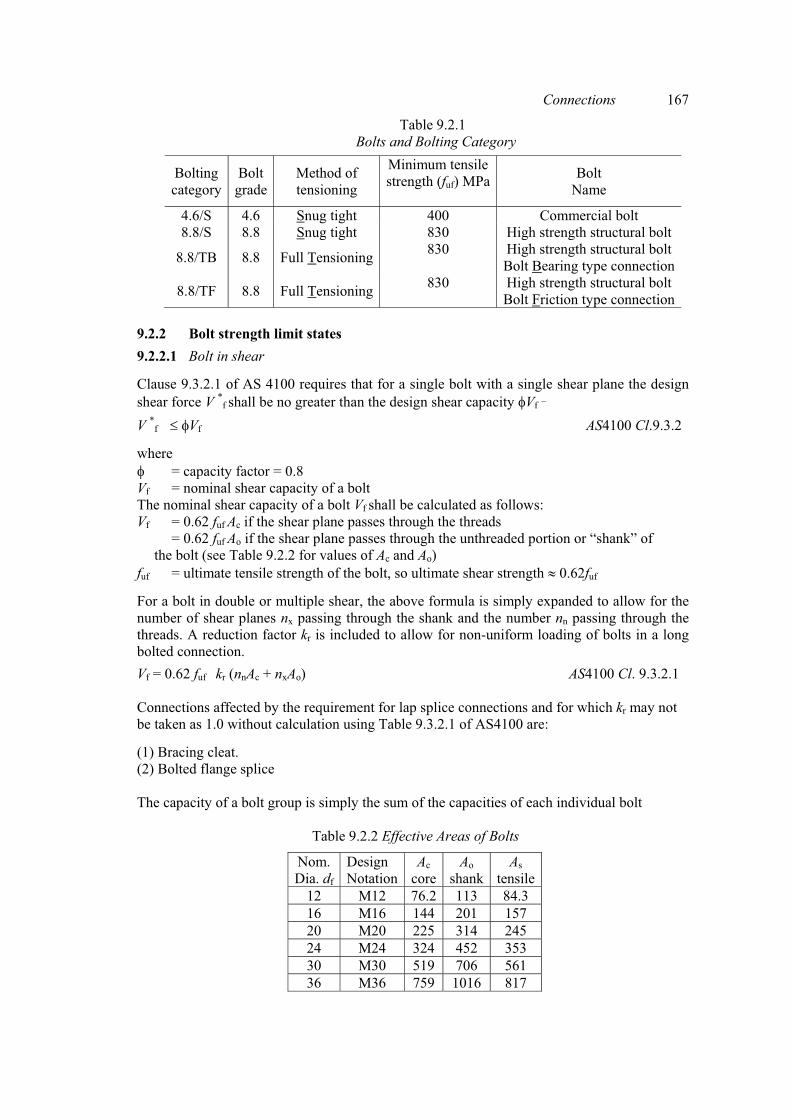
9.1 Introduction 166 9.2 Design of Bolts 166

9.2.1 Bolts and Bolting Categories 169 9.2.2 Bolt Strength Limit States 167 9.2.2.1 Bolt in Shear 167 9.2.2.2 Bolt in Tension 168 9.2.2.3 Bolt Subject to Combined Shear and Tension 168

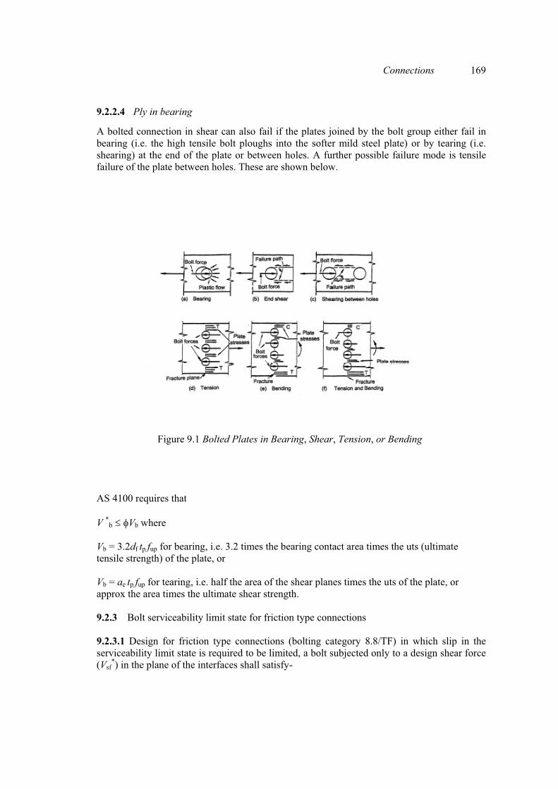
9.2.2.4 Ply in Bearing 169 9.2.3 Bolt Serviceability Limit State for Friction Type Connections 169

Contents vii

9.2.4 Design Details for Bolts and Pins 170 9.3 Design of Welds 171 9.3.1 Scope 171 9.3.1.1 Weld Types 171 9.3.1.2 Weld Quality 171 9.3.2 Complete and Incomplete Penetration Butt Weld 171 9.3.3 Fillet Welds 171 9.3.3.1 Size of a Fillet Weld 171

9.3.3.2 Capacity of a Fillet Weld 171 9.4 Worked Examples 173 9.4.1 Flexible Connections 173

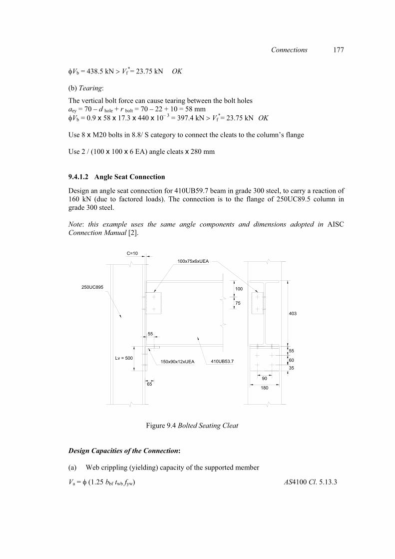
9.4.1.1 Double Angle Cleat Connection 173 9.4.1.2 Angle Seat Connection 177 9.4.1.3 Web Side Plate Connection 181

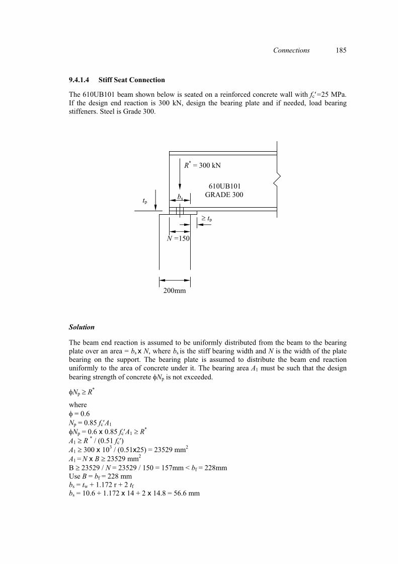
9.4.1.4 Stiff Seat Connection 185 9.4.1.5 Column Pinned Base Plate 187

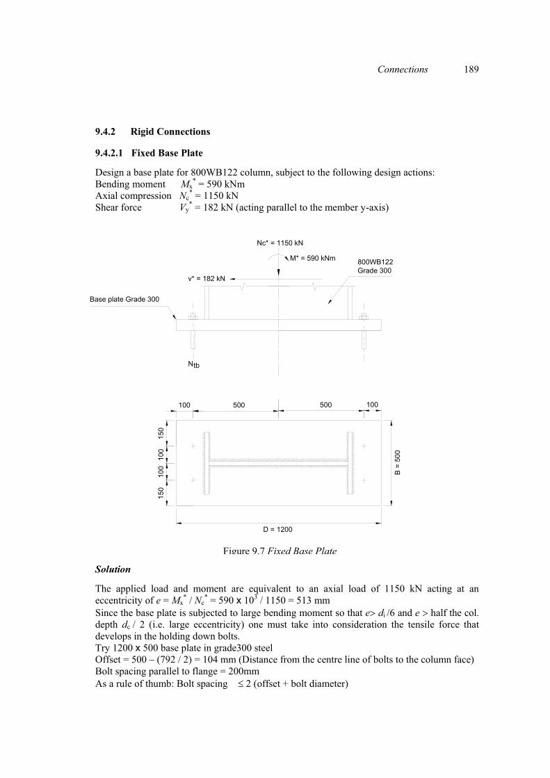
9.4.2 Rigid Connections 189 9.4.2.1 Fixed Base Plate 189

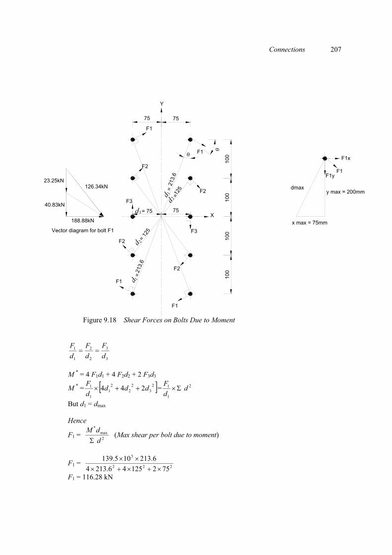
9.4.2.2 Welded Moment Connection 199 9.4.2.3 Bolted Moment Connection 206 9.4.2.4 Bolted Splice Connection 209

9.4.2.5 Bolted End Plate Connection (Standard Knee Joint) 213 9.4.2.6 Bolted End Plate Connection (Non-Standard Knee Joint) 226

9.5 References 229

viii

PREFACE___________________________________________________________________________

This book introduces the design of steel structures in accordance with AS 4100, the Australian Standard, in a format suitable for beginners. It also contains guidance and worked examples on some more advanced design problems for which we have been unable to find simple and adequate coverage in existing works to AS 4100. The book is based on materials developed over many years of teaching undergraduate engineering students, plus some postgraduate work. It follows a logical design sequence from problem formulation through conceptual design, load estimation, structural analysis to member sizing (tension, compression and flexural members and members subjected to combined actions) and the design of bolted and welded connections. Each topic is introduced at a beginner’s level suitable for undergraduates and progresses to more advanced topics. We hope that it will prove useful as a textbook in universities, as a self-instruction manual for beginners and as a reference for practitioners. No attempt has been made to cover every topic of steel design in depth, as a range of excellent reference materials is already available, notably through ASI, the Australian Steel Institute (formerly AISC). The reader is referred to these materials where appropriate in the text. However, we treat some important aspects of steel design, which are either: (i) not treated in any books we know of using Australian standards, or (ii) treated in a way which we have found difficult to follow, or (iii) lacking in straightforward, realistic worked examples to guide the student or

inexperienced practitioner. For convenient reference the main chapters follow the same sequence as AS 4100 except that the design of tension members is introduced before compression members, followed by flexural members, i.e. they are treated in order of increasing complexity. Chapter 3 covers load estimation according to current codes including dead loads, live loads, wind actions, snow and earthquake loads, with worked examples on dynamic loading due to vortex shedding, crane loads and earthquake loading on a lattice tank stand. Chapter 4 gives some examples and diagrams to illustrate and clarify Chapter 4 of AS 4100. Chapter 5 treats the design of tension members including wire ropes, round bars and compound tension members. Chapter 6 deals with compression members including the use of frame buckling analysis to determine the compression member effective length in cases where AS 4100 fails to give a safe design. Chapter 7 treats flexural members, including a simple explanation of criteria for classifying cross sections as fully, partially or laterally restrained, and an example of an I beam with unequal flanges which shows that the approach of AS 4100 does not always give a safe design. Chapter 8 deals with combined actions including examples of (i) in-plane member capacity using plastic analysis, and (ii) a beam-column with a tapered web. In Chapter 9, we discuss various existing models for the design of connections and present examples of some connections not covered in the AISC connection manual. We give step-by-step procedures for connection design, including options for different design cases. Equations are derived where we consider that these will clarify the design rationale. A basic knowledge of engineering statics and solid mechanics, normally covered in the first two years of an Australian 4-year B.Eng program, is assumed. Structural analysis is treated only briefly at a conceptual level without a lot of mathematical analysis, rather than using the traditional analytical techniques such as double integration, moment area and moment distribution. In our experience, many students get lost in the mathematics with these methods and they are unlikely to use them in practice, where the use of frame analysis software

Preface ix

ix

packages has replaced manual methods. A conceptual grasp of the behaviour of structures under load is necessary to be able to use such packages intelligently, but knowledge of manual analysis methods is not. To minimise design time, Excel spreadsheets are provided for the selection of member sizes for compression members, flexural members and members subject to combined actions. The authors would like to acknowledge the contributions of the School of Engineering at Griffith University, which provided financial support, Mr Jim Durack of the University of Southern Queensland, whose distance education study guide for Structural Design strongly influenced the early development of this book, Rimco Building Systems P/L of Arundel, Queensland, who have always made us and our students welcome, Mr Rahul Pandiya a former postgraduate student who prepared many of the figures in AutoCAD, and the Australian Steel Institute. Finally, the authors would like to thank their wives and families for their continued support during the preparation of this book.

Brian Kirke Iyad Al-Jamel June 2011

x

NOTATION________________________________________________________________________________ The following notation is used in this book. In the cases where there is more than one meaning to a symbol, the correct one will be evident from the context in which it is used. Ag = gross area of a cross-section An = net area of a cross-section Ao = plain shank area of a bolt As = tensile stress area of a bolt; or = area of a stiffener or stiffeners in contact with a flange

Aw = gross sectional area of a web ae = minimum distance from the edge of a hole to the edge of a ply measured in the direction of the component of a force plus half the bolt diameter. d = depth of a section de = effective outside diameter of a circular hollow section df = diameter of a fastener (bolt or pin); or = distance between flange centroids dp = clear transverse dimension of a web panel; or = depth of deepest web panel in a length d1 = clear depth between flanges ignoring fillets or welds d2 = twice the clear distance from the neutral axes to the compression flange. E = Young’s modulus of elasticity, 200x103 MPa e = eccentricity F = action in general, force or load fu = tensile strength used in design fuf = minimum tensile strength of a bolt fup = tensile strength of a ply fuw = nominal tensile strength of weld metal fy = yield stress used in design fys = yield stress of a stiffener used in design G = shear modulus of elasticity, 80x103 MPa; or = nominal dead load I = second moment of area of a cross-section Icy = second moment of area of compression flange about the section minor

principal y- axis

Notation xi

Im = I of the member under consideration Iw = warping constant for a cross-section Ix = I about the cross-section major principal x-axis Iy = I about the cross-section minor principal y-axis J = torsion constant for a cross-section ke = member effective length factor kf = form factor for members subject to axial compression kl = load height effective length factor kr = effective length factor for restraint against lateral rotation

l = span; or, = member length; or, = segment or sub-segment length le /r = geometrical slenderness ratio lj = length of a bolted lap splice connection Mb = nominal member moment capacity

Mbx = Mb about major principal x-axis Mcx = lesser of Mix and Mox

Mo = reference elastic buckling moment for a member subject to bending

Moo = reference elastic buckling moment obtained using le = l

Mos = Mob for a segment, fully restrained at both ends, unrestrained against lateral rotation and loaded at shear centre Mox = nominal out-of-plane member moment capacity about major principal x-axis Mpr = nominal plastic moment capacity reduced for axial force Mprx = Mpr about major principal x-axis Mpry = Mpr about minor principal y-axis Mrx = Ms about major principal x-axis reduced by axial force Mry = Ms about minor principal y-axis reduced by axial force Ms = nominal section moment capacity Msx = Ms about major principal x-axis Msy = Ms about the minor principal y-axis Mtx = lesser of Mrx and Mox

xii Notation

M* = design bending moment Nc = nominal member capacity in compression Ncy = Nc for member buckling about minor principal y-axis

Nom = elastic flexural buckling load of a member Nomb = Nom for a braced member Noms = Nom for a sway member Ns = nominal section capacity of a compression member; or = nominal section capacity for axial load Nt = nominal section capacity in tension Ntf = nominal tension capacity of a bolt

N* = design axial force, tensile or compressive nei = number of effective interfaces Q = nominal live load Rb = nominal bearing capacity of a web Rbb = nominal bearing buckling capacity Rby = nominal bearing yield capacity Rsb = nominal buckling capacity of a stiffened web Rsy = nominal yield capacity of a stiffened web r = radius of gyration ry = radius of gyration about minor principle axis. S = plastic section modulus s = spacing of stiffeners Sg = gauge of bolts Sp = staggered pitch of bolts t = thickness; or = thickness of thinner part joined; or = wall thickness of a circular hollow section; or = thickness of an angle section tf = thickness of a flange tp = thickness of a plate ts = thickness of a stiffener tw = thickness of a web tw, tw1, tw2 = size of a fillet weld

Notation xiii

Vb = nominal bearing capacity of a ply or a pin; or = nominal shear buckling capacity of a web Vf = nominal shear capacity of a bolt or pin – strength limit state Vsf = nominal shear capacity of a bolt – serviceability limit state Vu = nominal shear capacity of a web with a uniform shear stress distribution Vv = nominal shear capacity of a web Vvm = nominal web shear capacity in the presence of bending moment Vw = nominal shear yield capacity of a web; or = nominal shear capacity of a pug or slot weld V* = design shear force V*

b = design bearing force on a ply at a bolt or pin location V*

f = design shear force on a bolt or a pin – strength limit state V*

w = design shear force acting on a web panel yo = coordinate of shear centre Z = elastic section modulus Zc = Ze for a compact section Ze = effective section modulus

�b = compression member section constant

�c = compression member slenderness reduction factor

�m = moment modification factor for bending

�s = slenderness reduction factor.

�v = shear buckling coefficient for a web

�e = modifying factor to account for conditions at the far ends of beam members � = compression member factor defined in Clause 6.3.3 of AS 4100 � = compression member imperfection factor defined in Clause 6.3.3 of AS 4100 � = slenderness ratio �e = plate element slenderness

�ed = plate element deformation slenderness limit �ep = plate element plasticity slenderness limit �ey = plate element yield slenderness limit

xiv Notation

�n = modified compression member slenderness �s = section slenderness �sp = section plasticity slenderness limit �sy = section yield slenderness limit � = Poisson’s ratio, 0.25 � = Icy/Iy � = capacity factor

1

1 INTRODUCTION:THE STRUCTURAL DESIGN PROCESS__________________________________________________________________________________

1.1 PROBLEM FORMULATION

Before starting to design a structure it is important to clarify what purpose it is to serve. This may seem so obvious that it need not be stated, but consider for example a building, e.g. a factory, a house, hotel, office block etc. These are among the most common structures that a structural engineer will be required to design. Basically a building is a box-like structure, which encloses space. Why enclose the space? To protect people or goods? From what? Burglary? Heat? Cold? Rain? Sun? Wind? In some situations it may be an advantage to let the sun shine in the windows in winter and the wind blow through in summer (Figure1.1). These considerations will affect the design.

Figure 1.1 Design to use sun, wind and convection How much space needs to be enclosed, and in what layout? Should it be all on ground level for easy access? Or is space at a premium, in which case multi-storey may be justified (Figure1.2). How should the various parts of a building be laid out for maximum convenience? Does the owner want to make a bold statement or blend in with the surroundings? The site must be assessed: what sort of material will the structure be built on? What local government regulations may affect the design? Are cyclones, earthquakes or snow loads likely? Is the environment corrosive?

1.2 CONCEPTUAL DESIGN

Architects rather than engineers are usually responsible for the problem formulation and conceptual design stages of buildings other than purely functional industrial buildings. However structural engineers are responsible for these stages in the case of other industrial

Introduction 2

structures, and should be aware of the issues involved in these early stages of designing buildings. Engineers sometimes accuse architects of designing weird structures that are not sensible from a structural point of view, while architects in return accuse structural engineers of being concerned only with structural issues and ignoring aesthetics and comfort of occupiers. If the two professions understand each other’s points of view it makes for more efficient, harmonious work.

Figure1.2 Low industrial building and high rise hotel

The following decisions need to be made:

1. Who is responsible for which decisions? 2. What is the basis for payment for work done? 3. What materials should be used for economy, strength, appearance, thermal and sound

insulation, fire protection, durability? The architect may have definite ideas about what materials will harmonise with the environment, but it is the engineer who must assess their functional suitability.

4. What loads will the structure be subjected to? Heavy floor loads? Cyclones? Snow? Earthquakes? Dynamic loads from vibrating machinery? These questions are firmly in the engineer’s territory.

Besides buildings, other types of structure are required for various purposes, for example to hold something vertically above the ground, such as power lines, microwave dishes, wind turbines or header tanks. Bridges must span horizontally between supports. Marine structures such as jetties and oil platforms have to resist current and wave forces. Then there are moving steel structures including ships, trucks and railway rolling stock, all of which are subjected to dynamic loads.

Once the designer has a clear idea of the purpose of the structure, he or she can start to propose conceptual designs. These will usually be based on some existing structure, modified to suit the particular application. So the more you notice structures around you in everyday life the better equipped you will be to generate a range of possible conceptual designs from which the most appropriate can be selected.

Introduction 3

For example a tower might be in the form of a free standing cantilever pole, or a guyed pole, or a free-standing lattice (Figure1.3). Which is best? It depends on the particular application. Likewise there are many types of bridges, many types of building, and so on.

Figure1.3 Towers Left: “Tower of Terror” tube cantilever at Dream World theme park, Gold Coast. Right: bolted angle lattice transmission tower.

1.3 CHOICE OF MATERIALS Steel is roughly three times more dense than concrete, but for a given load-carrying capacity, it is roughly 1/3 as heavy, 1/10 the volume and 4 times as expensive. Therefore concrete is usually preferred for structures in which the dead load (the load due to the weight of the structure itself) does not dominate, for example walls, floor slabs on the ground and suspended slabs with a short span. Concrete is also preferred where heat and sound insulation are required. Steel is generally preferable to concrete for long span roofs and bridges, tall towers and moving structures where weight is a penalty. In extreme cases where weight is to be minimised, the designer may consider aluminium, magnesium alloy or FRP (fibre reinforced plastics, e.g. fibreglass and carbon fibre). However these materials are much more expensive again. The designer must make a rational choice between the available materials, usually but not always on the basis of cost. Although this book is about steel structures, steel is often used with concrete, not only in the form of reinforcing rods, but also in composite construction where steel beams support concrete slabs and are connected by shear studs so steel and concrete behave as a single structural unit (Figs.1.4, 1.5). Thus the study of steel structures cannot be entirely separated from concrete structures.

Introduction 4

Figure1.4 Steel bridge structure supporting concrete deck, Adelaide Hills

Figure1.5 Composite construction: steel beams supporting concrete slab in Sydney Airport car park

1.4 ESTIMATION OF LOADS (STRUCTURAL DESIGN ACTIONS) Having decided on the overall form of the structure (e.g. single level industrial building, high rise apartment block, truss bridge, etc.) and its location (e.g. exposed coast, central business district, shielded from wind to some extent by other buildings, etc.), we can then start to estimate what loads will act on the structure. The former SAA Loading code AS 1170 has now been replaced by AS/NZS 1170, which refers to loads as “structural design actions.” The main categories of loading are dead, live, wind, earthquake and snow loads. These will be discussed in more detail in Chapter 2. A brief overview is given below. 1.4.1 Dead loads or permanent actions (the permanent weight of the structure itself). These

can be estimated fairly accurately once member sizes are known, but these can only be determined after the analysis stage, so some educated guesswork is needed here, and numbers may have to be adjusted later and re-checked. This gets easier with experience.

Introduction 5

1.4.2 Live loads (imposed actions) are loads due to people, traffic etc. that come and go. Although these do not depend on member cross sections, they are less easy to estimate and we usually use guidelines set out in the Loading Code AS 1170.1

1.4.3 Wind loads (wind actions) will come next. These depend on the geographical region –

whether it is subject to cyclones or not, the local terrain – open or sheltered, and the structure height.

1.4.4 Earthquake and snow loads can be ignored for some structures in most parts of Australia, but it is important to be able to judge when they must be taken into account.

1.4.5 Load combinations (combinations of actions). Having estimated the maximum loads

we expect could act on the structure, we then have to decide what load combinations could act at the same time. For example dead and live load can act together, but we are unlikely to have live load due to people on a roof at the same time as the building is hit by a cyclone. Likewise, wind can blow from any direction, but not from more than one direction at the same time. Learners sometimes make the mistake of taking the most critical wind load case for each face of a building and applying them all at the same time. If we are using the limit state approach to design, we will also apply load factors in case the loads are a bit worse than we estimated. We can then arrive at our design loads (actions).

1.5 STRUCTURAL ANALYSIS

Once we know the shape and size of the structure and the loads that may act on it, we can then analyse the effects of these loads to find the maximum load effects (action effects), i.e. axial force, shear force, bending moment and sometimes torque on each member. Basic analysis of statically determinate structures can be done using the methods of engineering statics, but statically indeterminate structures require more advanced methods. Before desktop computers and structural analysis software became generally available, methods such as moment distribution were necessary. These are laborious and no longer necessary, since computer software can now do the job much more quickly and efficiently. An introduction to one package, Spacegass, is provided in this book. However it is crucial that the designer understands the concepts and can distinguish a reasonable output from a ridiculous output, which indicates a mistake in data input. 1.6 MEMBER SIZING, CONNECTIONS AND DOCUMENTATION After the analysis has been done, we can do the detailed design – deciding what cross section each member should have in order to be able to withstand the design axial forces, shear forces and bending moments. The principles of solid mechanics or stress analysis are used in this stage. As mentioned above, dead loads will depend on the trial sections initially assumed, and if the actual member sections differ significantly from those originally assumed it will be necessary to adjust the dead load and repeat the analysis and member sizing steps. We also have to design connections: a structure is only as strong as its weakest link and there is no point having a lot of strong beams and columns etc that are not joined together properly. Finally, we must document our design, i.e. provide enough information so someone can build it. In the past, engineers generally provided dimensioned sketches from which draftsmen prepared the final drawings. But increasingly engineers are expected to be able to prepare their own CAD drawings.

6

2 STEEL PROPERTIES ___________________________________________________________________________

2.1 INTRODUCTION To design effectively it is necessary to know something about the properties of the material. The main properties of steel, which are of importance to the structural designer, are summarised in this chapter.

2.2 STRENGTH, STIFFNESS AND DENSITY

Steel is the strongest, stiffest and densest of the common building materials. Spring steels can have ultimate tensile strengths of 2000 MPa or more, but normal structural steels have tensile and compressive yield strengths in the range 250-500 MPa, about 8 times higher than the compressive strength and over 100 times the tensile strength of normal concrete. Tempered structural aluminium alloys have yield strengths around 250 MPa, similar to the lowest grades of structural steel. Although yield strength is an important characteristic in determining the load carrying capacity of a structural element, the elastic modulus or Young’s modulus E, a measure of the stiffness or stress per unit strain of a material, is also important when buckling is a factor, since buckling load is a function of E, not of strength. E is about 200 GPa for carbon steels, including all structural steels except stainless steels, which are about 5% lower. This is about 3 times that of Aluminium and 5-8 times that of concrete. Thus increasing the yield strength or grade of a structural steel will not increase its buckling capacity. The specific gravity of steel is 7.8, i.e. its mass is about 7.8 tonnes/m3, about three times that of concrete and aluminium. This gives it a strength to weight ratio higher than concrete but lower than structural aluminium.

2.3 DUCTILITY Structural steels are ductile at normal temperatures under normal conditions. This property has two important implications for design. First, high local stresses due to concentrated loads or stress raisers (e.g. holes, cracks, sudden changes of cross section) are not usually a major problem as they are with high strength steels, because ductile steels can yield locally and relive these high stresses. Some design procedures rely on this ductile behaviour. Secondly, ductile materials have high “toughness,” meaning that they can absorb energy by plastic deformation so as not to fail in a sudden catastrophic manner, for example during an earthquake. So it is important to ensure that ductile behaviour is maintained. The factors affecting brittle fracture strength are as follows:

(1) Steel composition, including grain size of microscopic steel structures, and the steel temperature history.

(2) Temperature of the steel in service. (3) Plate thickness of the steel. (4) Steel strain history (cold working, fatigue etc.) (5) Rate of strain in service (speed of loading). (6) Internal stress due to welding contraction.

Steel Properties 7

In general slow cooling of the steel causes grain growth and a reduction in the steel toughness, increasing the possibility of brittle fracture. Residual stresses, resulting from the manufacturing process, reduce the fracture strength, whilst service temperatures influence whether the steel will fail in brittle or ductile manner.

2.3.1 Metallurgy and transition temperature

Every steel undergoes a transition from ductile behaviour (high energy absorption, i.e. toughness) to brittle behaviour (low energy absorption) as its temperatures falls, but this transition occurs at different temperatures for different steels, as shown in Fig.2.1 below. For low temperature applications L0 (guaranteed “notch ductile” down to 0�C) or L15 (ductile down to -15�C) should be specified. Figure 2.1 Impact energy absorption capacity and ductile to brittle transition temperatures of steels as a function of manganese content (adapted from Metals Handbook [1])

2.3.2 Stress effects Ductile steel normally fails by shearing or slipping along planes in the metal lattice. Tensile stress in one direction implies shear stress on planes inclined to the direction of the applied stress, as shown in Fig.2.2, and this can be seen in the necking that occurs in the familiar tensile test specimen just prior to failure. However if equal tensile stress is applied in all three principal directions the Mohr’s circle becomes a dot on the tension axis and there is no shear stress to produce slipping. But there is a lot of strain energy bound up in the material, so it will reach a point where it is ready to fail suddenly. Thus sudden brittle fracture of steel is most likely to occur where there is triaxial tensile stress. This in turn is most likely to occur in heavily welded, wide, thick sections where the last part of a weld to cool will be unable to contract as it cools because it is restrained in all directions by the solid metal around it. It is therefore in a state of residual triaxial tensile stress and will tend to pull apart, starting at any defect or crack.

-50 -25 0 25 50 75 100 125 150 0

50

100

150

200

250

300 2% Mn 1% Mn

0.5% Mn

0% Mn

Temperature, oC

Impa

ct e

nerg

y, J

8 Steel Properties

A B C

A

B

C

Tensile stress axis

Shear stress axis Mohr’s circle for uniaxial tension: Only tension on plane A, but both tension and shear on planes B and C

uniaxial tension

Mohr’s circle for triaxial tension: tension on all planes, but no shearto cause slipping

Figure 2.2 Uniaxial or biaxial tension produces shear and slip, but uniform triaxial tension does not

2.3.3 Case study: King’s St Bridge, Melbourne

The failure of King’s St Bridge in Melbourne in 1962 provided a good example of brittle fracture. One cold morning a truck was driving across the bridge when one of the main girders suddenly cracked (Fig.2.3). Nobody was injured but the subsequent enquiry revealed that some of the above factors had combined to cause the failure.

Figure 2.3 Brittle Crack in King’s St. Bridge Girder, Melbourne

Steel Properties 9

1. A higher yield strength steel than normal was used, and this steel was less ductile and had a higher brittle to ductile transition temperature than the lower strength steels the designers were accustomed to.

2. Thick (50 mm) cover plates were welded to the bottom flanges of the bridge girders to increase their capacity in areas of high bending moment.

3. These cover plates were correctly tapered to minimise the sudden change of cross section at their ends (Fig.2.2), but the welding sequence was wrong in some cases: the ends were welded last, and this caused residual triaxial tensile stresses at these critical points where stresses were high and the abrupt change of section existed.

Steelwork can be designed to avoid brittle fracture by ensuring that welded joints impart low restraint to plate elements, since high restraint could initiate failure. Also stress concentrations, typically caused by notches, sharp re-entrant angles, abrupt changes in shape or holes should be avoided.

2.4 CONSISTENCY The properties of steel are more predictable than those of concrete, allowing a greater degree of sophistication in design. However there is still some random variation in properties, as shown in Fig.2.4.

0

10

20

30

40

50

60

70

80

0.9 1 1.1 1.2 1.3 1.4 1.5 1.6

Ratio of measured yield stress to nominal

Freq

uenc

y

0

20

40

60

80

100

120

0.9 0.95 1 1.05

Ratio of actual to nominal flange thickness

Freq

uenc

y

Figure2.4 Random variation in measured properties of nominally identical steel specimens (adapted from Byfield and Nethercote [2])

10 Steel Properties

0

50

100

150

200

-50 -25 0 25 50 75 100 125

Temperature C

Impa

ct e

nerg

y, J

Although steel is usually assumed to be a homogeneous, isotropic material this is not strictly true, as all steel includes microscopic impurities, which tend to be preferentially oriented in the direction of mill rolling. This results in lower toughness perpendicular to the plane of rolling (Fig.2.5).

Figure 2.5 Lower toughness perpendicular to the plane of rolling (Metals Handbook [1])

Some impurities also tend to stay near the centre of the rolled item due to their preferential solubility in the liquid metal during solidification, i.e. near the centre of rolled plate, and at the junction of flange and web in rolled sections. The steel microstructure is also affected by the rate of cooling: faster cooling will result in smaller crystal grain sizes, generally resulting in some increase in strength and toughness. (Economical Structural Steel Work [3]) As a result, AS 4100 [4] Table 2.1 allows slightly higher yield stresses than those implied by the steel grade for thin plates and sections, and slightly lower yield stresses for thick plates and sections. For example the yield stress for Grade 300 flats and sections less than 11 mm thick is 320 MPa, for thicknesses from 11 to 17 mm it is 300 MPa and for thicknesses over 17 mm it is 280 MPa.

2.5 CORROSION Normal structural steels corrode quickly unless protected. Corrosion protection for structural steelwork in buildings forms a special study area. If the structural steelwork of a building includes exposed surfaces (to a corrosive environment) or ledges and crevices between abutting plates or sections that may retain moisture, then corrosion becomes an issue and a protection system is then essential. This usually involves consultation with specialists in this area. The choice of a protection system depends on the degree of corrosiveness of the environment. The cost of protection varies and is dependent on the significance of the structure, its ease of access for maintenance as well as the permissible frequency of maintenance without inconvenience to the user. Depending on the degree of corrosiveness of the environment, steel may need:

Variation of Charpy V-notch impact energy with notch orientation and temperature for steel plate containing 0.012% C.

Steel Properties 11

� Epoxy paint � ROZC (red oxide zinc chromate) paint � Cold galvanising (i.e. a paint containing zinc, which acts as a sacrificial coating, i.e. it

corrodes more readily than steel) � Hot dip galvanising (each component must be dipped in a bath of molten zinc after

fabrication and before assembly) � Cathodic protection, where a negative electrical potential is maintained in the steel, i.e.

an oversupply of electrons that stops the steel losing electrons and forming Fe ++ or Fe +++ and hence an oxide.

� Sacrificial anodes, usually of zinc, attached to the structure, which lose electrons more readily than the steel and so keep the steel supplied with electrons and inhibit oxide formation.

2.6 FATIGUE STRENGTH The application of cyclic load to a structural member or connection can result in failure at a stress much lower than the yield stress. Unlike aluminium, steel has an “endurance limit” for applied stress range, below which it can withstand an indefinite number of stress cycles, as shown in Fig 2.6. However Fig.2.6 oversimplifies the issue and the assessment of fatigue life of a member or connection involves a number of factors, which may be listed as follows:

(1) Stress concentrations (2) Residual stresses in the steel. (3) Welding causing shrinkage strains. (4) The number of cycles for each stress range. (5) The temperature of steel in service. (6) The surrounding environment in the case of corrosion fatigue.

For most static structures fatigue is not a problem, but fatigue calculations are usually carried out for the design of structures subjected to many repetitions of large amplitude stress cycles such as railway bridges, supports for large rotating equipment and supports for large open structures subject to wind oscillation.

Figure 2.6 Stress cycles to failure as a function of stress level

(adapted from Mechanics of Materials [5])

Number of completely reversed cycles

400

Steel (1020HR)

Aluminium (2024)

103 104 105 106 107 108 109

100

200

300

Stre

ss (M

Pa)

12 Steel Properties

To be able to design against fatigue, information on the loading spectrum should be obtained, based on research or documented data. If this information is not available, then assumptions must be made with regard to the nature of the cyclic loading, based on the design life of the structure. A detailed procedure on how to design against fatigue failure is outlined in Section 11 of AS4100 [4].

2.7 FIRE RESISTANCE Although steel is non-combustible and makes no contribution to a fire it loses strength and stiffness at temperatures exceeding about 200oC. Fig.2.7 shows the twisted remains of a steel framed building gutted by fire.

Figure 2.7 Remains of a steel framed building gutted by fire, Ashmore, Gold Coast Regulations require a building structure to be protected from the effects of fire to allow a sufficient amount of time before collapse for anyone in the building to leave and for fire fighters to enter if necessary. Additionally, it ought to delay the spread of fire to adjoining property. Australian Building Regulations stipulate fire resistance levels (FRL) for structural steel members in many types of applications.

The fire resistance level is a measure of the time, in minutes; it will take before the steel heats up to a point where the building collapses. The FRL required for a particular application is related to,

� the likely fire load inside the building (this relates to the amount of combustible

material in the building) � the height and area of the building � the fire zoning of the building locality and the onsite positioning.

In order to achieve the fire resistance periods, (specified in the Building Regulations) systems of fire protection are designed and tested by their manufactures. A fire protection system consists of the fire protection material plus the manner in which it is attached to the steel member. Apart from insulating structural elements, building codes call for fireproof

Steel Properties 13

walls (in large open structures) at intervals to reduce the hazard of a fire in one area spreading to neighbouring areas.

There is a range of fire protection systems to choose from, such as non-combustible paints or encasing steel columns in concrete. The manufactures of these materials can provide the necessary accreditation and technical data for them. These should be references to tests conducted at recognised fire testing stations. Their efficiency for achieving the required FRL as well as the cost of these materials should be taken into consideration. Concerning the protection of steel, the most feasible way is to cover or encase the bare steelwork in a non-combustible, durable, and thermally protective material. In addition, the chosen material must not produce smoke or toxic gases at an elevated temperature. These may be either sprayed onto the steel surface, or take the form of prefabricated casings clipped round the steel section.

2.8 REFERENCES 1. Metals Handbook, Vol.1 (1989). American Society for Metals, Metals Park, Ohio. 2. Byfield and Nethercote (1997). The Structural Engineer, Vol.75, No.21, 4 Nov. 3. Australian Institute of Steel Construction (1996). Economical Structural Steelwork, 4th edn. 4. Standards Australia (1998). AS 4100 – Steel Structures. 5. Beer, F.P. and Johnston, E.R. (1992). Mechanics of Materials, 2nd edn. SI Units.

14

3 LOAD ESTIMATION ___________________________________________________________________________

3.1 INTRODUCTION

Before any detailed sizing of structural elements can start, it is necessary to start to estimate the loads that will act on a structure. Once the designer and the client have agreed on the purpose, size and shape of a proposed structure and what materials it is to be made of, the process of load estimation can begin. Loads will always include the self-weight of the structure, called the “dead load.” In addition there may be “live” loads due to people, traffic, furniture, etc., that may or may not be present at any given time, and also loads due to wind, snow, earthquakes etc. The required sizes of the members will depend on the weight of the structure but will also contribute to the weight. So load estimation and member sizing are to some extent an iterative process in which each affects the other. As the designer gains experience with a particular type of structure it becomes easier to predict approximate loads and member sizes, thereby reducing the time taken in trial and error. However the inexperienced designer can save time by intelligent use of some short cuts. For example the design of structures carrying heavy dead loads such as concrete slabs or machinery may be dominated by dead load. In this case it may be best to size the slabs or machinery first so the dead loads acting on the supporting structure can be estimated. On the other hand many steel-framed industrial buildings in warm climates where snow does not fall can be designed mainly on the basis of wind loads, since dead and live loads may be small enough in relation to the wind load to ignore for preliminary design purposes. The wind load can be estimated from the dimensions of the structure and its location. Members can then be sized to withstand wind loads and then checked to make sure they can withstand combinations of dead, live and wind load. Where snowfall is significant, snow loads may be dominant. Earthquake loads are only likely to be significant for structures supporting a lot of mass, so again the mass should be estimated before the structural elements are sized. 3.2 ESTIMATING DEAD LOAD (G)

Dead load is the weight of material forming a permanent part of the structure, and in Australian codes it is given the symbol G. Dead load estimation is generally straightforward but may be tedious. The best way to learn how to estimate G is by examples. 3.2.1 Example: Concrete slab on columns Probably the simplest form of structure – at least for load estimation - is a concrete slab supported directly on a grid of columns, as shown in Fig.3.1.

Load Estimation 15

Figure 3.1 Concrete Slab on Columns Suppose the concrete (including reinforcing steel) weighs 25 kN/m3, the slab is 200 mm (0.2 m) thick, and the columns are spaced 4 m apart in both directions. We want to know how much dead load each column must support. First, we work out the area load, i.e. the dead weight G of one square metre of concrete slab. Each square m contains 0.2 m3 of concrete, so it will weigh 0.2x25 = 5 kN/m2 or G = 5 kPa. Next, we multiply the area load by the tributary area, i.e. the area of slab supported by one column. We assume that each piece of slab is supported by the column closest to it. So we can draw imaginary lines half way between each row of columns in each direction. Each internal column (i.e. those that are not at the edge of the slab) supports a tributary area of 16 m2, so the total dead load of the slab on each column is 16x5 = 80 kN. Assuming there is no overhang at the edges, edge columns will support a little over half as much tributary area because the slab will presumably come to the outer edge of the columns, so the actual tributary area will be 2.1x4 = 8.4 m2 and the load will be 42 kN. Corner columns will support 2.1x2.1 = 4.42 m2 and a load of 22.1 kN. To find the load acting on a cross-section at the bottom of each column where G is maximum, we must also consider the self-weight of the column. Suppose columns are 150UC30 sections (i.e steel universal columns with a mass of 30 kg/m, 4m high between the floor and the suspended slab. The weight of one column will therefore be 30x9.8/1000x4 = 1.2kN approximately. Thus the total load on a cross section of an internal column at the bottom will be 80 + 1.2 = 81.2 kN. If there are two or more levels, as in a multi-level car park or an office building, the load on each ground floor column would have to be multiplied by the number of floors. Thus if our car park has 3 levels, a bottom level internal column would carry a total dead load G = 3x81.2 = 243.6 kN.

(a) Perspective view (b) Plan view

16 Load Estimation

3.2.2 Concrete slab on steel beams and column A more common form of construction is to support the slab on beams, which are in turn supported on columns as shown in Figs.3.2 and 3.3 below. Because the beams are deeper and stronger than the slab, they can span further so the columns can be further apart, giving more clear floor space.

(a) Perspective (b) Plan View

Figure 3.2 Slab, Beams and Columns

Figure 3.3 Car parks. Left: Sydney Airport: concrete slabs on steel beams and concrete columns. Right: Petrie Railway Station, Brisbane: concrete slab on steel beams and steel columns

To calculate the dead load on the beams and columns, we now add another step in the calculation. Assuming we still have a 200mm thick slab, the area load due to the slab is still the same, i.e. 5 kPa.

Assume columns are still of 200x200mm section, at 4 m spacing in one direction. But we now make the slab span 4m between beams, and the beams span 8m between columns. So we have only half as many columns. But we now want to know the load on a beam. We could work out the total load on one 8m span of beam. But it is normal to work out a line load, i.e. the load per m along the beam. The tributary area for each internal beam in this case is a strip 4m wide, as shown in the diagram above. So the line load on the beam due to the slab only is 5 kN/m2 x 4 m = 20 kN/m. Note the units.

Load Estimation 17

We must also take into account the self-weight of the beam. Suppose the beams are 610UB101 steel universal beams weighing approximately 1 kN/m. The total line load G on the internal beams is now 20 + 1 = 21 kN/m. This will be the same on each floor because each beam supports only one floor. The lower columns take the load from upper floors but the beams do not. A line load diagram for an internal beam is shown in Fig.3.4 below. Note that we specify the span (8 m), spacing (4 m), load type (G) and load magnitude (21 kN/m).

Figure3.4 Line load diagram for Dead Load G on Beam

3.2.3 Walls Unlike car parks, most buildings have walls, and we can estimate their dead weight in the same way as we did with slabs, columns and beams. Sometimes walls are structural, i.e. they are designed to support load. Other walls may be just partitions, which contribute dead weight but not strength. These non-structural partition walls are common because it is very useful to be able to knock out walls and change the floor plan of a building without having to worry about it falling down. Suppose a wall is 100 mm thick and is made of reinforced concrete weighing 25 kN/m3. The weight will be 25 x 0.1 = 2.5 kN/m2 of wall area. If it is 4 m high, it will weigh 4m � 2.5 kN/m2 = 10 kN/m of wall sitting on the floor, i.e. the line load it will impose on a floor will be 10 kN/m. The SAA Loading Code AS 1170 Part 1, Appendix A, contains data on typical weights of building materials and construction. For example a concrete hollow block masonry wall 150 mm thick, made with standard aggregate, weighs about 1.73 kN/m2 of wall area. A 2.4 m high wall of this type of blocks will impose a line load of 1.73 � 2.4 = 4.15 kN/m.

3.2.4 Light steel construction Although the dead weight of steel and timber roofs and floors is much less than that of concrete slabs, it must still be allowed for. The principles are still the same: sheeting is supported on horizontal “beam” elements, i.e. members designed to withstand bending.

18 Load Estimation

However it is common in steel and timber roof and floor construction to have two sets of “beams,” i.e. flexural members, running at right angles to each other. These have special names, which are shown in the diagrams below.

3.2.5 Roof construction Corrugated metal (steel or aluminium) roof sheeting is normally supported on relatively light steel or timber members called purlins which run horizontally, i.e. at right angles to the corrugations which run down the slope. In domestic construction, tiled roofing is common. Tiles require support at each edge of each tile, so they are supported on light timber or steel members called battens, which serve the same purpose as purlins but are at much closer spacing, usually 0.3m. The purlins or battens are in turn supported on rafters or trusses. Rafters are heavier, more widely spaced steel or timber beams running at right angles to the purlins or battens, as shown in Fig.3.5, and spanning between walls or columns. Purlins usually span about 5 to 8 m and are usually spaced about 0.9 to 1.5 m apart. This spacing is dictated partly by the distance the sheeting can span between purlins, and partly by the fact that it is easier to erect a building if the purlins are close enough to be able to step from one to another before the sheeting is in place.

Figure 3.5 Roof Sheeting is Supported by Purlins, Rafters and Columns Trusses are commonly used to support battens in domestic construction. These are usually timber but may be made of light, cold-formed steel.

3.2.6 Floor construction Light floors are usually made of timber floor boards or sheets of particle board. Light floors are supported on floor joists, just as roof sheeting is supported on purlins or battens. Floor joists are typically spaced at 300, 450 or 600 mm centres and are in turn supported by bearers, as shown in Fig.3.7 below. Finally the whole floor is held up either by walls or by vertical columns called stumps. Note the similarity in principle between the roof structure shown in Fig.3.5 and the floor structure in Fig.3.6. This similarity is shown schematically in Fig.3.7.

Load Estimation 19

Figure 3.6 Typical Steel-Framed Floor Construction Showing Timber Sheeting and Steel Floor Joists, Bearers and Stumps

Figure 3.7 Similarity in Principle Between Floor and Roof Construction

3.2.7 Sample calculation of dead load G for a steel roof

We start by finding the weight of each component of the roof, i.e. - sheeting - purlins - rafters Let us assume the roof sheeting is “Custom Orb” (the normal corrugated steel sheeting) 0.48 mm thick. In theory we could work out the weight of this material from the density of steel, but we would need to allow for the corrugations and the overlap where sheets join. So it is simpler to look it up in a published table which includes these allowances, such as the one in Appendix A of this study guide. From this table, the weight of 0.48mm Orb is 5.68 kg/m2. Let us now assume this roof sheeting is supported on cold-formed steel Z section purlins of Z15019 section (i.e. 150 mm deep, made of 1.9 mm thick sheet metal formed into a Z profile. See Appendix B). This section weighs 4.46 kg/m. Assume the purlins are at 1.2 m centres (i.e. their centre lines are spaced 1.2 m apart). These purlins span 6 m between rafters of hot rolled 310UB40.4 section (the “310” means 310 mm deep, and the “40.4” means 40.4 kg/m). Assume the rafters span 10 m and are, of course spaced at 6 m centres, the same as the purlin span. This arrangement is shown in Fig.3.10.

20 Load Estimation

"Cold formed steel Z section" means a flat steel strip is bent so it cross section resembles a letter Z. This is done while the steel is cold, and the cold working increases its yield strength but decreases its ductility. Cold formed sections are usually made from thin (1 to 3 mm) galvanized steel. This contrasts with the heavier hot rolled I, angle and channel sections which are formed while hot enough to make the steel soft. Hot rolled sections are usually supplied "black," i.e. as-rolled, with no special surface finish or corrosion protection, so they usually have some rust on the surface.

Rafters @ 6000 crs

Purlins @1200 crs

1200

6000

Figure 3.8 Layout of Purlins and Rafters

3.2.7.1 Dead load on purlins

To calculate dead loads acting on purlins, the principles are the same as for concrete construction, i.e. 1. Work out area loads of roof sheeting 2. Multiply by the spacing of purlins to get line loads on purlins. In this case, the area load due to sheeting is 5.68 kg/m2 = 5.68 x 9.8 N/m2 = 5.68 x 9.8 / 1000 kN/m2 = 0.0557 kPa. The line load on the purlins due to sheeting will be 0.0557 kN/m2 x 1.2m = 0.0668 kN/m. But the total line load for G on purlins consists of the sheeting weight plus the purlin self-weight, which is 4.46 kg/m = 0.0437 kN/m. Thus the total line load due to dead weight G on the purlin is G = 0.0668 + 0.0437 = 0.11 kN/m. This is shown as a line load diagram in Fig.3.9 below, in the same form as the line load diagram for the beam in Fig.3.4.

Load Estimation 21

10,000

G = 0.948 kN/m

6000centres

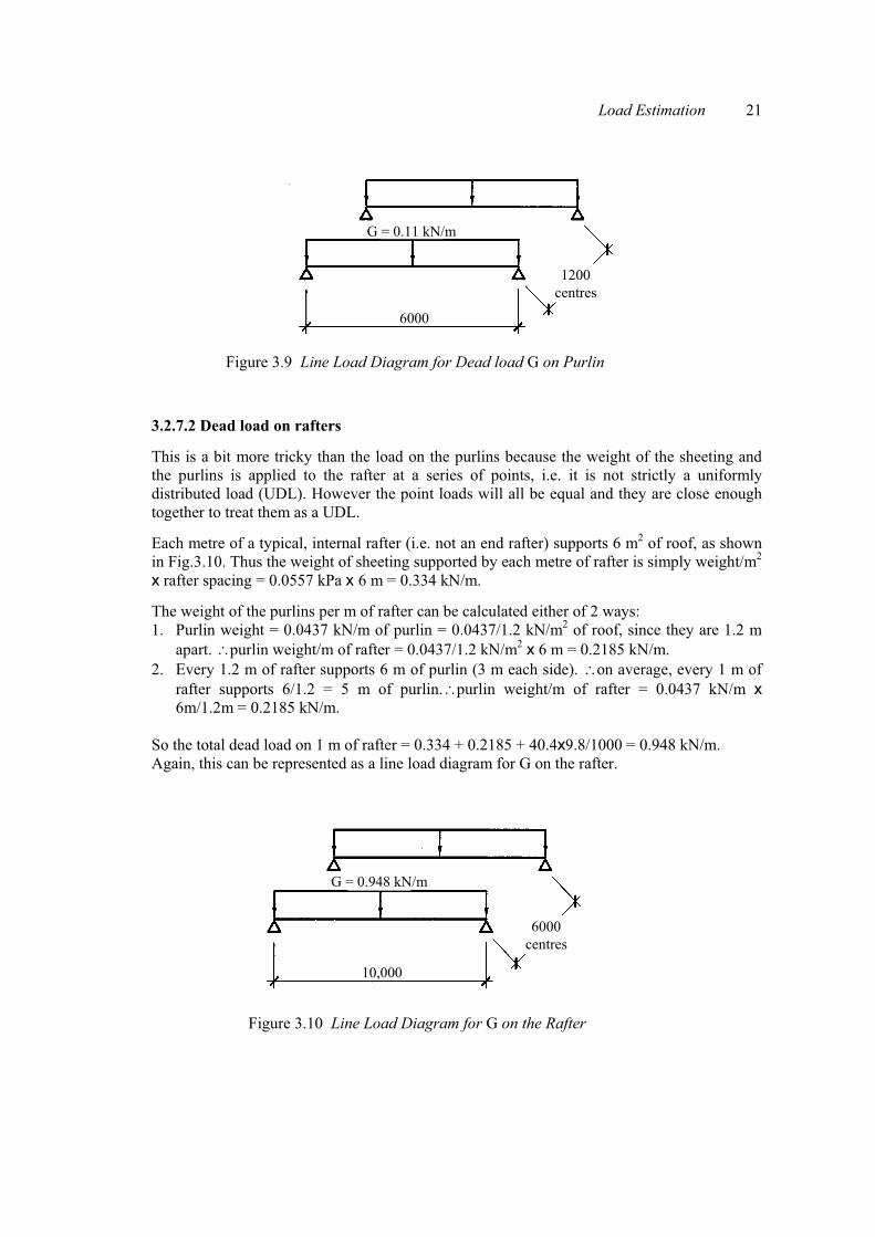
3.2.7.2 Dead load on rafters This is a bit more tricky than the load on the purlins because the weight of the sheeting and the purlins is applied to the rafter at a series of points, i.e. it is not strictly a uniformly distributed load (UDL). However the point loads will all be equal and they are close enough together to treat them as a UDL. Each metre of a typical, internal rafter (i.e. not an end rafter) supports 6 m2 of roof, as shown in Fig.3.10. Thus the weight of sheeting supported by each metre of rafter is simply weight/m2 x rafter spacing = 0.0557 kPa x 6 m = 0.334 kN/m. The weight of the purlins per m of rafter can be calculated either of 2 ways: 1. Purlin weight = 0.0437 kN/m of purlin = 0.0437/1.2 kN/m2 of roof, since they are 1.2 m

apart. purlin weight/m of rafter = 0.0437/1.2 kN/m2 x 6 m = 0.2185 kN/m. 2. Every 1.2 m of rafter supports 6 m of purlin (3 m each side). on average, every 1 m of

rafter supports 6/1.2 = 5 m of purlin.purlin weight/m of rafter = 0.0437 kN/m x 6m/1.2m = 0.2185 kN/m.

So the total dead load on 1 m of rafter = 0.334 + 0.2185 + 40.4x9.8/1000 = 0.948 kN/m. Again, this can be represented as a line load diagram for G on the rafter.

Figure 3.10 Line Load Diagram for G on the Rafter

6000

G = 0.11 kN/m

1200centres

Figure 3.9 Line Load Diagram for Dead load G on Purlin

22 Load Estimation

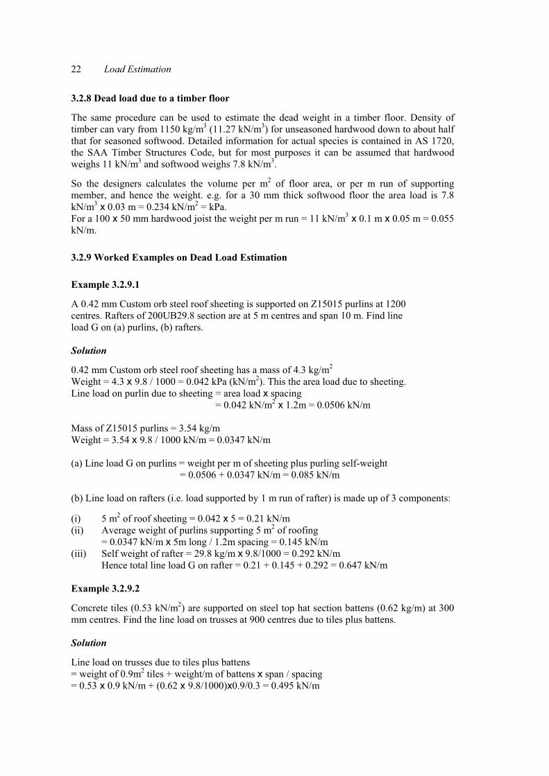
3.2.8 Dead load due to a timber floor

The same procedure can be used to estimate the dead weight in a timber floor. Density of timber can vary from 1150 kg/m3 (11.27 kN/m3) for unseasoned hardwood down to about half that for seasoned softwood. Detailed information for actual species is contained in AS 1720, the SAA Timber Structures Code, but for most purposes it can be assumed that hardwood weighs 11 kN/m3 and softwood weighs 7.8 kN/m3. So the designers calculates the volume per m2 of floor area, or per m run of supporting member, and hence the weight. e.g. for a 30 mm thick softwood floor the area load is 7.8 kN/m3 x 0.03 m = 0.234 kN/m2 = kPa. For a 100 x 50 mm hardwood joist the weight per m run = 11 kN/m3 x 0.1 m x 0.05 m = 0.055 kN/m.

3.2.9 Worked Examples on Dead Load Estimation Example 3.2.9.1

A 0.42 mm Custom orb steel roof sheeting is supported on Z15015 purlins at 1200 centres. Rafters of 200UB29.8 section are at 5 m centres and span 10 m. Find line load G on (a) purlins, (b) rafters. Solution 0.42 mm Custom orb steel roof sheeting has a mass of 4.3 kg/m2 Weight = 4.3 x 9.8 / 1000 = 0.042 kPa (kN/m2). This the area load due to sheeting. Line load on purlin due to sheeting = area load x spacing = 0.042 kN/m2 x 1.2m = 0.0506 kN/m Mass of Z15015 purlins = 3.54 kg/m Weight = 3.54 x 9.8 / 1000 kN/m = 0.0347 kN/m (a) Line load G on purlins = weight per m of sheeting plus purling self-weight = 0.0506 + 0.0347 kN/m = 0.085 kN/m (b) Line load on rafters (i.e. load supported by 1 m run of rafter) is made up of 3 components: (i) 5 m2 of roof sheeting = 0.042 x 5 = 0.21 kN/m (ii) Average weight of purlins supporting 5 m2 of roofing = 0.0347 kN/m x 5m long / 1.2m spacing = 0.145 kN/m (iii) Self weight of rafter = 29.8 kg/m x 9.8/1000 = 0.292 kN/m Hence total line load G on rafter = 0.21 + 0.145 + 0.292 = 0.647 kN/m Example 3.2.9.2 Concrete tiles (0.53 kN/m2) are supported on steel top hat section battens (0.62 kg/m) at 300 mm centres. Find the line load on trusses at 900 centres due to tiles plus battens.

Solution

Line load on trusses due to tiles plus battens = weight of 0.9m2 tiles + weight/m of battens x span / spacing = 0.53 x 0.9 kN/m + (0.62 x 9.8/1000)x0.9/0.3 = 0.495 kN/m

Load Estimation 23

Example 3.2.9.3 Softwood (7.8 kN/m3) purlins of 100x50 mm cross section at 3000 mm centres, spanning 4m, support Kliplok 406, 0.48 mm thick. Rafters at 4 m centres, spanning 6m, are steel 200x100x4 mm RHS. Find the line load G on (a) purlins, (b) rafters. Solution Sheeting: area load = 5.3 kg/m2 = 5.3x 9.8 /1000 kPa = 0.052 kPa Line load on purlin due to sheeting = area load x spacing = 0.052 x 3 = 0.156 kN/m Purlins: Softwood 7.8 kN/m3 Line load due to self weight = 7.8 kN/m3 x 0.1m x 0.05 m = 0.039 kN/m

(a) Total line load G on purlins = 0.156 + 0.039 = 0.195 kN/m Line load on rafter due to sheeting = area load x rafter spacing = 0.052 x 4 = 0.208 kN/m Line load on rafter due to purlins = purlin weight/m x rafter spacing / purlin spacing = 0.039 x 4 / 3 = 0.052 kN/m Line load on rafter due to self weight = 17.9 kg/m = 17.9 x 9.8 / 1000 = 0.175 kg/m

(b) Total line load G on rafters = 0.208 + 0.052 + 0.175 = 0.435 kN/m Example 3.2.9.4 19 mm thick hardwood flooring (11 kN/m3) is supported on 100x50 mm hardwood joists at 450 mm centres. The joists span 2 m between 200UB29.8 bearers, which span 3 m. Find line load G on (a) joists, (b) bearers. Find also the end reaction supported on the stumps. Solution

Area load due to 19 mm thick hardwood flooring (11 kN/m3) = 11 x 0.019 = 0.209 kPa Line load on joists at 450 crs due to flooring = 0.209 x 0.45 = 0.094 kN/m

Line load due to self weight of 100x50 mm hardwood joists = 11 kN/m3 x 0.1 x 0.05 = 0.055 kN/m (a) Total line load G on joists = 0.094 + 0.055 = 0.149 kN/m Line load on bearers at 2m crs due to flooring = 0.209 x 2 = 0.418 kN/m. Line load on bearers due to joists at 450 crs = 0.094 x 2 / 0.45 = 0.418 kN/m (coincidence) Line load due to bearer self-weight = 29.8 x 9.8/1000 = 0.292 kN/m. (b) Total line load G on bearers = 0.418 + 0.418 + 0.292 = 1.13 kN/m End reaction supported on the stumps: Bearers span 3 m, so total load which must be supported by 2 stumps = 1.13 kN/m x 3m = 3.39 kN Weight supported by each bearer (for this span only) = 3.39 / 2 = 1.7 kN (However internal stumps would support bearers on each side, so would support 3.39 kN)

24 Load Estimation

Example 3.2.9.5 A 150 mm thick solid reinforced concrete slab (25 kN/m3) is supported on 360UB50.7 beams at 2 m centres, spanning 4 m. Find line load G on beams.

Solution Area load due to 150 mm thick reinforced concrete slab (25 kN/m3) = 0.15x25 = 3.75 kN/m2 Line load on beams at 2 m centres due to slab = 3.75 kN/m2 x 2m = 7.5 kN/m Line load on beams due to self weight = 50.7 x 9.8 /1000 = 0.497 kN/m Hence total line load G on beams = 7.5 + 0.497 = 8.00 kN/m

3.3 ESTIMATING LIVE LOAD Q It would be possible to estimate the maximum number of people that might be expected in a particular room, calculate their total weight and divide by the area of the room. For example you might expect about 30 people averaging 80 kg in a small lecture room 8 x 5 m in area, i.e. approximately 30 x 80 kg = 2400 kg in 40 m2 = 60 kg/m2 = 0.588 kPa. But it is possible that many more might be in the room for some special occasion. It is physically possible to squeeze about 6 people into a 1 m square, i.e. about 6 x 80 kg/m2 = 4.7 kPa. But it is most unlikely that there would ever be 6 people/m2 in every part of a room. So what figure should we use? Fortunately the loading code AS/NZS 1170.1:2002 [1] gives guidelines for live loads on roofs and floors.

3.3.1 Live load Q on a roof Live loads on “non-trafficable” roofs such as the roof of a portal frame building arrises mainly from maintenance loads where new or old roof sheeting may be stacked in concentrated areas. For purlins and rafters, the code provides for a distributed load of 0.25 kN/m2 where the supported area A is greater than or equal to 14 m2, the area A being the plan projection of the inclined roof surface area. For areas A less than 14 m2, the code specifies the distributed load of wQ = [1.8/A + 0.12] kN/m2 on the plan projection. In addition to the distributed live load, the loading code also specifies that portal frame rafters be designed for a concentrated load of 4.5 kN at any point, this concentrated load is usually assumed to act at the ridge.

3.3.2 Live load Q on a floor

This is very simple to calculate. Floor live loads are given in AS1170.1. For example a floor in a normal house must be designed for an area load Q = 1.5 kPa (i.e. approximately 150 kg per m2 of floor area. In addition, it must be designed to take a “point” load of 1.8 kN on an area of 350 mm2. Usually the area load governs the design. Suppose a house has floor joists at 300 mm centres. These must be designed for a live load of 1.5 kN/m2 x 0.3 m = 0.45 kN/m. If the bearers are at 2.4 m centres, the live load will be 1.5 x 2.4 = 3.6 kN/m. 3.3.3 Other live loads These may include impact and inertia loads due to highly active crowds, vibrating machinery, braking and horizontal impact in car parks, cranes, hoists and lifts. AS 1170.1 gives guidance on design loads due to braking and horizontal impact in car parks. Other dynamic loads are treated in other standards such as the Crane and Hoist Code AS 1418. Some of these will be treated later in this chapter.

Load Estimation 25

3.3.4 Worked Examples on Live Load Estimation Example 3.3.4.1

A 0.42 mm Custom orb steel roof sheeting is supported on Z15015 purlins at 1200 centres. Rafters of 200UB29.8 section are at 5 m centres and span 10 m. Find line load Q on (a) purlins, (b) rafters. Solution (a) Each purlin span supports an area A = 5 x 1.2 = 6 m2

wQ = [1.8/A + 0.12] = 0.42 kN/m2 AS 1170.1 Cl 4.8.1.1 Line load Q on purlin = 0.42x1.2 = 0.504 kN/m (b) Each rafter span supports an area of 5 x10 = 50 m2 > 14 m2 wQ = 0.25 kPa AS 1170.1 Cl 4.8.1.1 Line load Q on rafter = 0.25 x 5 = 1.25 kN/m 0.504 kN/m 1.25 kN/m _____________________________ _____________________________

Line Loads for Live Load Q (left) for Purlin, (right) for Rafter

Example 3.3.4.2

19 mm thick hardwood flooring is supported on 100x50 mm hardwood joists at 450 mm centres. The joists span 2 m between 200UB29.8 bearers, which span 3 m. Find line load Q on (a) joists, (b) bearers. If it is a normal house floor (Q = 1.5 kPa). Solution Area load Q (normal house) = 1.5 kPa (a) Line load Q on joist = 1.5 x 0.45 = 0.675 kN/m (b) Line load Q on bearers = 1.5 x 2 = 3 kN/m Example 3.3.4.3

A 150 mm thick solid reinforced concrete slab is supported on 360UB50.7 beams at 2 m centres, spanning 4 m. Find line load Q on (a) a 1 m wide strip of floor, (b) beams if it is a library reading room (Q = 2.5 kPa). Solution

(a) Line load Q on a 1 m wide strip of floor = 2.5 kN/m2 x 1m = 2.5 kN/m (b) Line load Q on beams at 2 m centres = 2.5 x 2 = 5 kN/m

5 m 10 m

26 Load Estimation

3.4 WIND LOAD ESTIMATION

Relative motion between fluids (e.g. air and water) and solid bodies causes lift, drag and skin friction forces on the solid bodies. Examples include lift on an aeroplane wing, drag on a moving vehicle, force exerted by a flowing river on a bridge pylon, and wind loads on structures. The estimation of wind loads is a complex problem because they vary greatly and are influenced by a large number of factors. The following introduction is intended only to illustrate the procedure for estimating wind loads on rectangular buildings and lattice towers. For a more complete treatment the reader should consult wind loading codes and specialist references. 3.4.1 Factors influencing wind loads

Wind forces increase with the square of the wind speed, and wind speed varies with geographical region, local terrain and height. Tropical coastal areas are subject to tropical cyclones, and structures in these areas must be designed for higher wind speeds than those in other areas. Wind speed generally increases with height above the ground, and winds are stronger in more exposed locations such as hilltops, foreshores and flat treeless plains than in sheltered inner city locations. Thus tall structures and structures in exposed locations must be designed for higher wind gusts than low structures and those in sheltered locations. The pressure exerted by the wind on any part of a structure depends on the shape of the structure and the wind direction. Windward walls and upwind slopes of steeply pitched roofs experience a rise in pressure above atmospheric pressure, while side walls, leeward walls, leeward slopes of roofs and flat roofs experience suction on the outside. The greatest suction pressures tend to occur near the edges of roofs and walls. This is shown in Fig.3.11 below.

pressure

suctionwind

leeward or side opening:internal suction

pressure

suctionwind

Windward opening: internal pressure

Figure 3.11 Internal Pressure can be either Positive or Negative, Depending on Location of Openings Relative to Wind Direction

Load Estimation 27

Internal pressure is positive (pushing the walls and roof outwards) if there is a dominant opening on the windward side only, and negative (sucking inwards) if the openings are on a side or leeward wall. The extreme storm wind gusts are the ones that do the damage, and these are very variable in time and space, as shown in Fig.3.12 below. Statistically it is most unlikely that the pressure from an extreme gust will act over a large area of a building all at the same time, so design pressures on small areas are greater than those on large areas. (Of course the total force is more on a large area). All of these factors are taken into account in design codes.

Figure3.12 External Pressure Distribution Varies with Time due to Turbulence and Gustiness of the wind. Codes must use a simplified envelope. [2]

28 Load Estimation

3.4.2 Design wind speeds

It is important to design structures so they will not collapse completely or disintegrate and allow sharp pieces to fly through the air. Most of the loss of life in the 1974 Darwin cyclone was caused by flying roof sheeting. At the same time it is uneconomic to design structures so strong that they will remain totally undamaged even in an extreme storm that may occur on average only once in hundreds of years. Thus it is normal to use two wind speeds in design: one for ultimate strength design, which is unlikely to occur during the structure’s life but could occur at any time. In this wind some minor damage is acceptable but the structure must not totally collapse. A lower wind speed is used to design for serviceability, in which the structure should survive without damage. The discussion below will follow the current Australian and New Zealand wind loading code, AS/NZS 1170.2:2002 [3], which represents a major revision of the previous AS1170.2, and will deal mainly with rectangular buildings, although lattice towers will also be treated. The procedure is summarised in the flow charts in Figs.3.13 and 3.14. To determine site wind speed Vsit,� for each of the 4 wind directions perpendicular to the faces of the building (Fig.2.2)

� 1. Determine geographical region (A1 – A7, W, B, C, D), hence regional wind speed VR (Table 3.1)

�

2. Determine wind direction multiplier Md (Table 3.2) for each of the 4 wind directions.

�

Is there significant shielding by other buildings? If yes, determine shielding multiplier Ms (Clause 4.3). If not, Ms = 1.

Mz,cat (Tables 4.1(A), 4.1(B)). For low buildings take height z = average roof height. For high buildings tabulate Mz,cat for each floor level.

Determine local terrain category from 1 (very exposed) to 4 (very sheltered) (Clause 4.2.1).

�

Is the building on a hill or escarpment? If yes, determine topographical multiplier Mt (Clause 4.4). If not, Mt = 1.

�

Hence determine site wind speed for each orthogonal wind direction Vsit,� = VR Md (Mz,cat Ms Mt).

Figure 3.13 Flow Chart to Determine Site Wind speed Vsit,�

Load Estimation 29

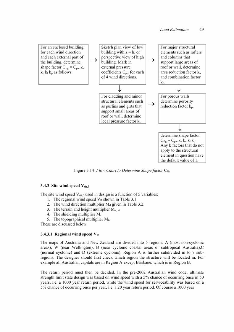
For an enclosed building, for each wind direction and each external part of the building, determine shape factor Cfig = Cp,e ka kc kl kp as follows:

�

Sketch plan view of low building with z = h, or perspective view of high building. Mark in external pressure coefficients Cp,e for each of 4 wind directions.

�

For major structural elements such as rafters and columns that support large areas of roof or wall, determine area reduction factor ka and combination factor kc.

� �For cladding and minor structural elements such as purlins and girts that support small areas of roof or wall, determine local pressure factor kl.

�

For porous walls determine porosity reduction factor kp.

�

determine shape factor Cfig = Cp,e ka kc kl kp Any k factors that do not apply to the structural element in question have the default value of 1.

Figure 3.14 Flow Chart to Determine Shape factor Cfig

3.4.3 Site wind speed Vsit,�

The site wind speed Vsit,� used in design is a function of 5 variables: 1. The regional wind speed VR shown in Table 3.1. 2. The wind direction multiplier Md given in Table 3.2. 3. The terrain and height multiplier Mz,cat 4. The shielding multiplier Ms 5. The topographical multiplier Mt.

These are discussed below.

3.4.3.1 Regional wind speed VR

The maps of Australia and New Zealand are divided into 5 regions: A (most non-cyclonic areas), W (near Wellington), B (near cyclonic coastal areas of subtropical Australia),C (normal cyclonic) and D (extreme cyclonic). Region A is further subdivided in to 7 sub-regions. The designer should first check which region the structure will be located in. For example all Australian capitals are in Region A except Brisbane, which is in Region B. The return period must then be decided. In the pre-2002 Australian wind code, ultimate strength limit state design was based on wind speed with a 5% chance of occurring once in 50 years, i.e. a 1000 year return period, while the wind speed for serviceability was based on a 5% chance of occurring once per year, i.e. a 20 year return period. Of course a 1000 year

30 Load Estimation

return period does not imply that this wind speed will occur once every 1000 years. It should rather be considered as a 0.1% probability of occurring in any year. In the 2002 code the choice of return period is not specified, and regional wind speeds VR are listed for each region and for return periods ranging from 5 to 2000 years (Table 3.1). The discussion which follows is based on V1000, the same as the old strength limit state. For Brisbane V1000 = 60 m/s and for all other Australian capital cities V1000 = 48 m/s.

3.4.3.2 Wind direction multiplier Md For regions A and W, stronger winds come from some directions, so wind direction multipliers Md are provided for 8 wind directions (Table 3.2). Thus for example Sydney is in Region A2, where the strongest winds come from the west, where the direction multiplier Md = 1, while Md for north, north east and east is only 0.8. So structures in Sydney must be designed for a regional wind speed of 46�1 = 46 m/s from the west, but only 46�0.8 = 36.8 m/s from the north or east. For regions B, C and D it is assumed that the maximum wind speed is the same for all directions.

3.4.3.3 The terrain and height multiplier Mz,cat Terrain is classified into 4 categories, ranging from 1 for very open exposed terrain, through to 4 for well sheltered sites. Most built up areas are classified as Category 3. Mz,cat decreases from category 1 to 4, and increases with height z above ground level (Tables 4.1(A), 4.1(B)). For small buildings z is taken as the average height of the roof, while for tall buildings it is normal to calculate different values of Mz,cat at different heights up the building (Fig.2.1). Thus for example a house 5 m high in a Sydney suburb (Region A, z = 5m, cat 3) would have Mz,cat = 0.83, while the top of a 50 m high structure on a fairly exposed site in Sydney (Region A, z = 50m, cat 2) would have Mz,cat = 1.18.

3.4.3.4 Other multipliers

The shielding multiplier Ms allows for a reduced design wind speed on structures which are shielded by adjacent buildings, while the topographical multiplier Mt provides for increased wind speeds on hilltops and escarpments. A detailed discussion of these factors is outside the scope of this book and the reader is advised to study the code for further information. When the above 5 variables have been evaluated for a particular site and wind direction in Regions A and W, the orthogonal design wind speeds Vdes,� for the 4 faces of a rectangular building can be determined by interpolating between the wind speeds in the “cardinal wind directions”. For example the top of the 50 m high building mentioned above is located in Region A2, with V1000 = 46 m/s, Md as shown below, Mz,cat = 1.18, assuming Ms and Mt = 1, would have a site wind speed for west wind given by Vsit,� = VR Md (Mz,cat Ms Mt) = 46 � 1 � (1.18 � 1 � 1) = 54.3 m/s. Site wind speeds for the other cardinal directions are tabulated in Table 3.1 and graphed in Fig.3.15:

Load Estimation 31

Table 3.1 Site Wind speeds for the 8 Cardinal Directions for One Particular Site in Sydney

Wind direction Vsit,�, m/s

N 46 � 0.8 � (1.18 � 1 � 1) = 43.4 NE 46 � 0.8 � (1.18 � 1 � 1) = 43.4 E 46 � 0.8 � (1.18 � 1 � 1) = 43.4

SE 46 � 0.95 � (1.18 � 1 � 1) = 51.6 S 46 � 0.9 � (1.18 � 1 � 1) = 48.9

SW 46 � 0.95 � (1.18 � 1 � 1) = 51.6 W 46 � 1 � (1.18 � 1 � 1) = 54.3

NW 46 � 0.95 � (1.18 � 1 � 1) = 51.6

Figure 3.15 Variation of Site Wind Speed with Direction for one Particular Site in Sydney These site wind speeds are shown in Fig.3.16 below on a plan view of a proposed building and the procedure for calculating the design wind speed for one face of that building is outlined (the wording in the code is hard to follow without an example). The East-North East face of the building has been selected to illustrate the procedure. Taking a 45� arc each side of the normal to the building face, and interpolating linearly between the wind speeds for the adjacent cardinal directions gives 43.4 m/s for NNE and 47.5 m/s for ESE. The greater of these is 47.5 m/s so this is taken as the design wind speed for this face of the building. Likewise the design wind speeds for the other 3 faces would be NNW 43.4 m/s, WSW 53.0 m/s, SSE 50.2 m/s.

Site wind speeds, Sydney, Mz,cat = 1.18

0

10

20

30

40

50

60

N NE E SE SE SW W NW

cardinal directions

win

d sp

eed,

m/s

32 Load Estimation

45°

45°

N: 43.4 m/s NE: 43.4 m/s

E:43.4 m/s

SE: 51.6 m/s

S: 48.8 m/s

SW: 51.6 m/s

W: 54.3 m/s

NW: 51.6 m/s

Interpolate: ESE 47.5 m/s

Interpolate: NNE 43.4 m/s

Figure 3.16 Site Wind Speeds Used for Interpolation,Building at 22.5� to Cardinal Directions If the faces of the building form other angles with the cardinal directions the same procedure is followed, using linear interpolation. Thus for example a building face oriented 10� south of west would have the 45� lines oriented 35� north of west and 55� south of west, respectively, as shown in Fig.3.17 below. The values of site wind speed for these 45� directions would be obtained by interpolation between the adjacent cardinal points, and the maximum wind speed within that 90� would be used for design. In this case that maximum is 54.3 m/s for due west.

Figure 3.17 Site Wind Speeds Used tor Interpolation, Building at any Angle to Cardinal Directions

45°

45°

N: 43.4 m/s NE: 43.4 m/s

E:43.4 m/s

SE: 51.6 m/s

S: 48.8 m/s

SW: 51.6 m/s

W: 54.3 m/s

NW: 51.6 m/s

Interpolate: 51.0 m/s

Interpolate: 52.2 m/s

10°

Load Estimation 33

3.4.4 Aerodynamic shape factor

Having determined the design wind speed, two more variables must be evaluated before the design wind pressure on any surface of a structure can be determined. These are the aerodynamic shape factor Cfig, which is itself a function of several variables, and the dynamic response factor Cdyn. Cdyn = 1 unless the structure is “wind sensitive”, i.e. has a natural frequency less than 1 Hz. The aerodynamic shape factor Cfig is defined in Clause 5.2 for enclosed buildings as Cfig = Cp,e ka kc kl kp for external pressures Cfig = Cp,i kc for external pressures Cfig = Cf kc for frictional drag forces For freestanding walls, hoardings, canopies and roofs Cfig = Cp,n ka kl kp for pressures normal to the surface Cfig = Cf for frictional drag forces where Cp,e = external pressure coefficient Cp,e, ka = area reduction factor kc = combination factor kl = local pressure factor kp = porous cladding reduction factor Cp,i = internal pressure coefficient Cf = frictional drag force coefficient Cp,n = net pressure coefficient acting normal to the surface for canopies etc. 3.4.5 Calculating external pressures Values of Cp,e vary over the external surface of the building and depend on the structure’s shape and the orientation of the surface relative to the wind. For example the windward wall generally has Cp,e = +0.7, while the side walls near the windward end of a building have Cp,e = - 0.65. Other values are given in Tables 5.2(A), (B), (C), 5.3(A), (B) and (C). The design external pressure at a given point depends not only on the site wind speed and the external pressure coefficient, but also on the 4 factors ka, kc, kl and kp, which are explained below. The area reduction factor ka allows for the fact that peak wind gusts will not hit the whole of a building at the same time, so the bigger the area supported, the lower the average pressure. Thus large structural elements such as rafters and columns that support a big area of roof or wall can be designed for a smaller average pressure than can small elements such as purlins or girts. If you leave ka = 1 you will get a safe design but it may be conservative and therefore not the most economical. The combination factor kc, illustrated in Table 5.5 of the wind loading code, allows a reduction in design pressures for some situations where pressures acting on two or more surfaces of an enclosed building contribute to forces in a particular structural member, and are unlikely to be at their maximum values simultaneously. As with ka, the maximum allowable reduction is only 20% and a safe but conservative design is obtained by ignoring this factor.

34 Load Estimation

In contrast to ka and kc, the local pressure factor kl actually requires an increase in design pressure for small areas which may experience local extreme pressures. It applies only to cladding, purlins, girts and battens which support areas less than a2 where “a” is defined as the minimum of 0.2b, 0.2d and h, b and d being the plan dimensions and h the height of a rectangular building. The porous cladding reduction factor kp, as its name implies, allow for a reduction in design pressures if the cladding is porous, and ignoring it will produce a safe but conservative design. We are now in a position to calculate the aerodynamic shape factor Cfig and hence the design external pressures acting on each part of an enclosed building. Let us take as an example an industrial building 30 x 36 m in plan with eaves 5 m high and a ridge 7 m high, giving a roof pitch of 7.6�. Portal frames are at 6 m centres as shown in Fig.3.18 below, with purlins and girts at 1.2 m centres.

Values of Cp,e are shown in Fig.3.19 below for a cross wind (i.e. wind direction normal to long walls, defined as � = 0�).

Wind direction � = 0�

Rafters at 6 m centres

Ridgeheight 7 m

d =30 m

b = 36 m

Eaves height 5 m

Mean height 6 m

Figure 3.18 Plan View of Building Showing Dimensions

wind

6 m

6 m

12 m

6 m

+0.7

-0.65

-0.5

-0.9, -0.4

-0.5, 0

-0.3, +0.2-0.3

-0.2, +0.3

-0.2-0.5

Figure 3.19 Plan View of Building Showing Values of Cp,e for Cross Wind

Load Estimation 35

Area reduction factor ka

The rafters each support an area of 30�6 = 180 m2 of roof, so for the rafters ka = 0.8 (Table 5.4). The columns each support 30 m2 of wall, so for the columns ka = 0.9 approximately (interpolating in Table 5.4). For purlins, girts and cladding, ka = 1. The combination factor kc

Is tricky to evaluate, and it is argued below, always safe to ignore and best ignored in most cases. Clause 5.4.3 of AS 1170.2:2002 states that kc may be applied “where wind pressures acting on two or more surfaces of an enclosed building contribute simultaneously to a structural action effect on a major structural element.” Light portal frame buildings are the most common structures for which wind loads govern the design, and the action effect which determines member sizing is usually bending moment. The bending moment at any point in a statically indeterminate portal frame is influenced by loads on every member, i.e. it is true that “wind pressures acting on two or more surfaces … contribute simultaneously” to the bending moment. Thus it would appear at fist sight that kc should be evaluated. To do this for the portal frame building shown in Fig.3.18, we must look at an end elevation of the building: see Fig.3.20 below. This loading case corresponds to case (b) in Table 5.5, so it would appear that kc = 0.8, i.e. the design loads can be reduced by 20%. However this is not so.

According to Table 5.5, kc = 1 “where wind action from any single surface contributes 75% or more to an action effect.” Thus to evaluate kc it is necessary to perform an analysis of the portal frame with wind load applied to each single surface in turn to assess whether or not “wind action from any single surface contributes 75% or more” to the maximum bending moment in the frame. This was done for the frame shown in Fig.3.18 above for a typical but arbitrary wind loading, and as shown in Fig.3.21 below, it was found that

1. The bending moment due to wind load on the whole frame is 196 kNm at the windward rafter-column connection and 112 kNm at the leeward rafter-column connection,

2. The bending moment due to wind load on the upwind slope of the roof alone is 94 kNm at the windward rafter-column connection and 153 kNm at the leeward rafter-column connection.

Thus wind action on the upwind roof slope produces 153/196 = 78% of the maximum bending moment in the frame due to the combined actions. In this situation it seems prudent to use the conservative value of 1 for kc.

0.70.5

Table 5.5(b): kc = 0.8

Figure 3.20 End Elevation Showing Wind Pressure Coefficients Contributing to Action Combination Factor kc

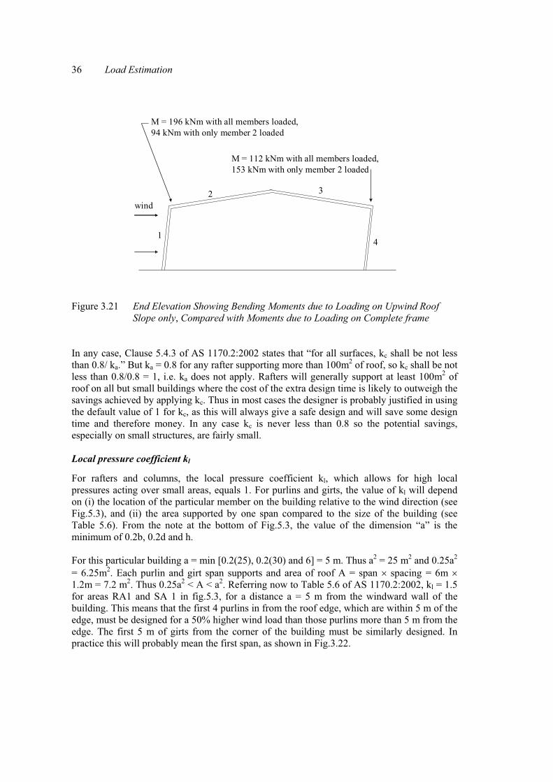
36 Load Estimation

Figure 3.21 End Elevation Showing Bending Moments due to Loading on Upwind Roof Slope only, Compared with Moments due to Loading on Complete frame In any case, Clause 5.4.3 of AS 1170.2:2002 states that “for all surfaces, kc shall be not less than 0.8/ ka.” But ka = 0.8 for any rafter supporting more than 100m2 of roof, so kc shall be not less than 0.8/0.8 = 1, i.e. ka does not apply. Rafters will generally support at least 100m2 of roof on all but small buildings where the cost of the extra design time is likely to outweigh the savings achieved by applying kc. Thus in most cases the designer is probably justified in using the default value of 1 for kc, as this will always give a safe design and will save some design time and therefore money. In any case kc is never less than 0.8 so the potential savings, especially on small structures, are fairly small. Local pressure coefficient kl

For rafters and columns, the local pressure coefficient kl, which allows for high local pressures acting over small areas, equals 1. For purlins and girts, the value of kl will depend on (i) the location of the particular member on the building relative to the wind direction (see Fig.5.3), and (ii) the area supported by one span compared to the size of the building (see Table 5.6). From the note at the bottom of Fig.5.3, the value of the dimension “a” is the minimum of 0.2b, 0.2d and h. For this particular building a = min [0.2(25), 0.2(30) and 6] = 5 m. Thus a2 = 25 m2 and 0.25a2 = 6.25m2. Each purlin and girt span supports and area of roof A = span � spacing = 6m � 1.2m = 7.2 m2. Thus 0.25a2 < A < a2. Referring now to Table 5.6 of AS 1170.2:2002, kl = 1.5 for areas RA1 and SA 1 in fig.5.3, for a distance a = 5 m from the windward wall of the building. This means that the first 4 purlins in from the roof edge, which are within 5 m of the edge, must be designed for a 50% higher wind load than those purlins more than 5 m from the edge. The first 5 m of girts from the corner of the building must be similarly designed. In practice this will probably mean the first span, as shown in Fig.3.22.

M = 196 kNm with all members loaded, 94 kNm with only member 2 loaded

1

2 3

4

M = 112 kNm with all members loaded, 153 kNm with only member 2 loaded

wind

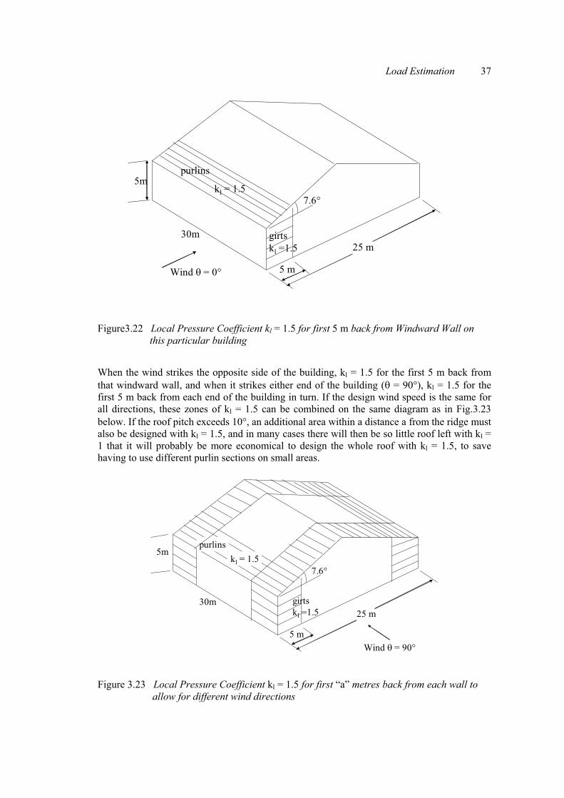
Load Estimation 37

Figure3.22 Local Pressure Coefficient kl = 1.5 for first 5 m back from Windward Wall on this particular building

When the wind strikes the opposite side of the building, kl = 1.5 for the first 5 m back from that windward wall, and when it strikes either end of the building (� = 90�), kl = 1.5 for the first 5 m back from each end of the building in turn. If the design wind speed is the same for all directions, these zones of kl = 1.5 can be combined on the same diagram as in Fig.3.23 below. If the roof pitch exceeds 10�, an additional area within a distance a from the ridge must also be designed with kl = 1.5, and in many cases there will then be so little roof left with kl = 1 that it will probably be more economical to design the whole roof with kl = 1.5, to save having to use different purlin sections on small areas.

25 m30m

7.6°

Wind � = 90�

5m

5 m

purlinskl = 1.5

girtskl =1.5

Figure 3.23 Local Pressure Coefficient kl = 1.5 for first “a” metres back from each wall to allow for different wind directions

25 m30m

7.6°

Wind � = 0�

5m

5 m

purlins

kl = 1.5

girtskl =1.5

38 Load Estimation

The permeable cladding reduction factor kp

This reduction factor allows for a small reduction in negative external pressures acting on a permeable wall with a solidity ratio between 0.1% and 1%. The code gives no indication what sorts of walls might have such a permeability, and the design will be safe if kp is taken as 1, i.e. ignored. Thus Cfig can now be calculated. For example for the columns in the windward side wall in Figs.3.21-3.25 above, Cfig = Cp,e ka kc kl kp = +0.7�0.9�1�1�1 = + 0.63 For the purlins within 5m of the roof edge, Cfig = Cp,e ka kc kl kp = -0.9�1�1�1.5�1 = -1.35

3.4.6 Calculating internal pressures

The internal pressure coefficient Cp,i, as shown in Fig.3.14 above, may be either positive or negative, depending on the location of openings relative to the wind. For buildings with open interior plan, Cp,i is assumed to be the same on all internal surfaces of an enclosed building at any given time. Values of Cp,I are given in Table 5.1(A) and (B) of AS 1170.2:2002. If there is just one dominant opening, Cp,i corresponds to the external pressure coefficient Cp,e that would apply on the face where the opening is located. Thus for example a shed with one end open will experience Cp,I = +0.7 when the wind blows directly into the open end, and Cp,i = -0.65 for a cross wind, as shown in Fig.3.24 below. If the building is enclosed, or has openings distributed around faces which have both positive and negative external pressures, internal pressure coefficients are smaller. To calculate internal pressures, look up internal pressure coefficients in Table 5.1 of AS 1170.2:2002 and multiply by the combination factor kc if applicable, then multiply by the dynamic pressure qz. It can be difficult to estimate Cp,i because most industrial buildings have large roller doors that can constitute “dominant openings” if open. A dominant opening, especially on the windward side of a building, makes a huge difference to internal pressures and hence to design wind loads, which usually dominate the design of light steel buildings. Hence they greatly affect the cost of a building. So the designer must decide whether to assume roller doors are shut or whether to allow for the possibility that one or more could be open. In cyclonic areas there is plenty of warning of normal tropical cyclones, so it can be assumed that roller doors can be closed before the cyclone hits the building, and the same applies to strong winds in non-cyclonic areas. However so-called “mini-cyclones” frequently strike without warning and do significant damage in some areas, such as South Eastern Queensland. (These are really microbursts associated with thunderstorms). If we assume the roller doors could be open in a mini-cyclone, or could fail in a cyclone, we have to allow for dominant openings. If they are on the windward side of the building they result in large positive internal pressures, which combine with large external suction pressures near the windward edge of the roof to cause very large uplift loads. However most engineers would not do this because it would result in an over-designed, uneconomical building. Statistically V1000 has a 0.1% chance of occurring in any one year, so it is unlikely that the building will ever experience it. But there is always a chance it will. So what do we do? One rationale for not allowing for full positive internal pressure is that the steel roof structure is ductile and will bend, distorting roof sheeting and allowing some equalisation of pressure between inside and outside before the roof literally flies away and starts killing people.

Load Estimation 39

Cp,i = +0.7 Cp,i = -0.65

Figure 3.24 Internal Pressure Coefficients Cp,i for a building with a dominant opening (shown in plan view)

3.4.7 Frictional drag The frictional drag force coefficient Cf ranges from 0.01 to 0.04 depending on the roughness of the surface. Unlike the pressure coefficients, Cf is used to calculate forces parallel to the building surface. Skin friction drag on buildings is easily calculated from Clause 5.5. Example

Wind blows parallel to the long walls of a building 6 m high, 50 m long and 20 m wide. Roof and wall sheeting have corrugations across the wind direction. qz = 2 kPa. Calculate the frictional drag. Solution

From Clause 5.5, h < b,area A = (b + 2h)x(d - 4h) = (20 + 12) x (50 – 24)m2 = 832 m2 Drag force coefficient Cf = 0.04 Ff = Cf qz A = 0.04 x 2 kPa x 832m2 = 66.6 kN 3.4.8 Net pressures

For enclosed buildings the design loads on structural elements are calculated from the most extreme net pressures, which are simply the algebraic sum of external and internal pressures. Care is necessary to get the signs right. For example positive pressure on both the outside and inside surfaces will tend to cancel out. For plane structures such as free roofs, canopies, awnings, hoardings, free standing walls, etc., the net pressure coefficient Cp,n takes the place of Cp,e and Cp,i. These are dealt within Appendix D of the code. 3.4.9 Exposed structural members

Drag forces on exposed structural members such as lattice towers are covered on Appendix E of the code.

40 Load Estimation

3.4.10 Worked Examples on Wind Load Estimation Example 3.4.10.1 List the basic wind speeds Vu for the following locations: (a) Perth (b) Cairns (c) Brisbane (d) Toowoomba. Solution

The regional wind speeds V1000 for the following locations (see AS 1170.2 Clause 3.4): (a) Perth: 46 m/s (Region A1) (b) Cairns 70Fc = 73.5 m/s (Region C) (c) Brisbane 60 m/s (Region B) (d) Toowoomba. 46 m/s (Region A4)

Example 3.4.10.2

Calculate the design wind speed Vdes,� and the dynamic wind pressure qz for the following sites, assuming Ms = Mt = 1: (a) A 7 m high portal frame building on an exposed site (cat 2) in Cairns, with b = 48 m and d = 15 m. Rafters at 6 m centres span 15 m. Purlins and girts are spaced at 1200 centres. (b) A 20 m high building on an exposed site in Pt Hedland, WA (Region D). For this flat roofed building, b = d = 15 m. (c) A 5 m high building in a built up area on the Gold Coast. (d) The upper portion of a 50 m high building on the Gold Coast without any significant shielding by adjacent structures. This building has a 30� roof pitch.

Solution (a) A 7 m high portal frame building on an exposed site in Cairns. V1000 = 73.5 m/s, Mz,cat = 0.97 (Table 4.1(B)), Vdes,� = 73.5 x 0.97 = 71.3 m/s and qz = 0.6 Vdes,�

2 x 10-3 kPa = 3.05 kPa (b) A 20 m high building on an exposed site in Pt Hedland, WA. V1000 = 85FD = 93.5 m/s, Mz,cat = 1.13 V des,� = 93.5 x 1.13 = 105.7 m/s and qz = 0.6 Vdes,�

2 x 10-3 kPa = 6.7 kPa (c) A 5 m high building in a built up area on the Gold Coast. Vu = 60 m/s, Mz,cat = 0.83 V des,� = 60 x 0.83 = 49.8 � 50 m/s and qz = 0.6 Vdes,�

2 x 10-3 kPa = 1.5 kPa

(d) The upper portion of a 50 m high building, with plan dimensions 30x30 m, roof pitch = 45�, wind direction � = 0�, on the Gold Coast, without any significant shielding by adjacent structures. Vu = 60 m/s, Mz,cat = 1.18 V des,� = 60 x1.18 = 70.8 m/s and qz = 0.6 Vdes,�

2 x 10-3 kPa = 3.0 kPa

Load Estimation 41

Example 3.4.10.3

Calculate the design external pressure pe for the following, assuming ka = kl = kp = 1: (a) The windward face of the building in Example 3.4.10.2(a). (b) The side wall near the windward face of the building in Example 3.4.10.2(a). (c) The windward portion of the roof of the building in Example 3.4.10.2(a) (roof pitch < 10�). (d) The leeward face of the building in Example 3.4.10.2(a). (e) The windward face of the building in Example 3.4.10.2(b).

(f) The windward portion of the roof of the building in Example 3.4.10.2(b)(roof pitch < 10�). (g) The windward portion of the roof of the building in Example 3.4.10.2(d) (roof pitch = 30�,� = 0).

Solution

(a) Referring to Table 5.2(A), height h < 25 m and this is not an elevated building. We are using a single value of qz,u = qh, the value at the top of the building, for the whole building. Cp,e = 0.7 for windward face of building qz = 3.05 kPa pe = Cp,eqz = + 0.7 x 3.05 = 2.14 kPa (b) Referring to Table 5.2(C), Cp,e = -0.65 pe = Cp,eqz = -0.65 x 3.05 = -1.98 kPa (c) Referring to Table 5.3(A), in this case the ratio of height h to depth d (plan dimension in direction of wind, see Fig.3.4.3) is 7/15 < 0.5 so Cp,e can vary from –0.9 to –0.4. Uplift is usually the critical load on roofs, so the worst case will be –0.9. pe = Cp,eqz = -0.9 x 3.05 = - 2.75 kPa

(d) Referring to Table 5.2(B), � = 0� with � < 10�, so use left hand side of table. Also, d / b < 1 (wind is hitting long face of building), so Cp,e = - 0.5. pe = Cp,eqz = - 0.5 x 3.05 = 1.53 kPa (e) qz = 6.7 kPa. Again this building is < 25 m high, qz = qh and it is not a highset building. pe = Cp,eqz = + 0.7 x 6.7 = 4.69 kPa (f) From part (e) above, qz, = 6.7 kPa. From Table 5.3(A), with h/d = 20/15 > 1 (extreme right side of table), Cp,e can range from –1.3 to –0.6. We will again take the maximum suction pressure. pe = Cp,eqz = -1.3 x 6.7 = -8.71 kPa (g) The windward portion of the roof of the building in Question 2(d) (roof pitch = 45�, � = 0).qz = 3.0 kPa From Table 5.3(B), with h / d = 50/30 > 1 and � = 45�, Cp,e = 0, 0.8sin� = 0, +0.57 pe = Cp,eqz = 0, +1.7 kPa.

42 Load Estimation

Example 3.4.10.4

Calculate the design external pressure pe (see Clause 2.4.1, AS 1170.2) for the following: (a) A purlin within 2 m of the windward face of the building in Question 2(a). (Consider kl).

(b) A rafter near the leeward end of the building in Question 2(a) for wind direction � = 90� (hitting the end of the building). (Consider ka).

Solution

(a) From Fig.5.3 in AS1170.2, dimension "a" is min. of 0.2 x 15 and 0.2 x 48 and 7 = 3 m. Referring to Table 5.6 in AS1170.2, case WA1 applies only to windward walls, i.e. not applicable. Case RA1 does apply: Each span of the purlin we are considering supports an area of roof = 6 x 1.2 = 7.2 m2 < 1.0a2 = 9 m2, and is within 2 m i.e. < distance "a" = 3 m from a roof edge. So kl = 1.5. Pe = 1.5 x (-3.05) (from Example 3.4.10.3 (c)) = - 4.6 kPa

(b) A rafter near the leeward end of the building in Example 3.4.10.2(a) for wind direction � = 90� (hitting the end of the building). The area supported by one rafter = 6 x 15 = 90 m2. So from Table 3.4.4 in AS1170.2, we can interpolate and take ka = 0.82 approx. Referring to Table 5.3(A) AS1170.2, with wind from end of building (� = 90�), and h/d = 7/48 < 1.0, Cp,e on downwind part of roof ranges from – 0.2 to + 0.2. For max uplift, Pe = 0.82 x (-0.2) x (3.05) (Example 3.4.10.3 (a)) = -0.50 kPa, or For max downward force, Pe = 0.82 x (+0.2) x (-3.05) = + 0.50 kPa. Example 3.4.10.5

For the building in Example 3.4.10.2, a roller door on the windward side is open and this is estimated to constitute a "dominant opening" 3 times bigger than the total of openings on other walls and roofs subject to external suction (Table 3.4.7 in AS1170.2). Calculate: (a) the internal pressure (b) the net pressure difference acting on the sheeting supported by the purlin in Example 3.4.10.4 (a) (c) the line load Wu on this purlin for ultimate strength design

(d) the net pressure difference acting on the sheeting supported by the rafter in Example 3.4.10.4 (b)

(e) the line load Wu on this rafter for ultimate strength design. Solution (a) For the building in Example 3.4.10.2 (a), a roller door on the windward side is open and this is estimated to constitute a "dominant opening" 3 times bigger than the total of openings on other walls and roofs subject to external suction (Table 5.1(A) in AS1170.2). Cp,i = 0.6 (a) the internal pressure = Cp,i qz = + 0.6 x 3.05 (from Example 3.4.10.3(a)) = + 1.83 kPa

Load Estimation 43

(b) the net pressure difference acting on the sheeting supported by the purlin in Question 4(a) is the difference between the answers in Example 3.4.10.4 (a) and 5(a), i.e. – 4.6 – (+1.83) = -6.43 kPa. (c) the line load Wu on this purlin for ultimate strength design = area load x purlin spacing = -6.43 kN/m2 x 1.2m = -7.72 kN/m (d) the net pressure difference acting on the sheeting supported by the rafter in Example 3.4.10.4 (b) is the difference between the answers in Example 3.4.10.4 (b) and 5(a), i.e. either –0.5 – (+1.83) = - 2.33 kPa or +0.5 – (+1.83) = - 1.33 kPa Clearly the first case is gives a larger wind load, but we would also have to consider the combination of wind and dead load. (e) the line load Wu on this rafter for ultimate strength design = area load x rafter spacing = -2.33 kN/m2 x 6m = -14 kN/m

Example 3.4.10.6 A building is to be constructed in a built-up industrial area at Ernest on the Gold Coast. It will be 5 m high, 30m long and 12 m wide, with a flat roof. Rafters spanning 12 m, at 5m centres, are to support purlins at 1 m centres. There will be 2 roller doors, each 4.5m wide and 4.5 m high, in the 2 middle bays on one long side of the building. Calculate the design wind load for ultimate strength on (a) the rafters (b) the purlins.

Solution

1. Region B, assume importance level = 2, so return period = 500 years and regional wind speed VR = V500 = 57 m/s (Table 3.1, AS/NZS 1170.2:2002).

2. Terrain category 3 (normal built up area). 3. Height = 5 m. 4. Terrain and structure height multiplier Mz,cat = 0.83 (Table 4.1(A)). 5. Assume Shielding multiplier & Topographic multiplier = 1. 6. Calculate Design wind speed Vdes,� = VR M(z,cat) Ms Mt = 57 x 0.83 x 1 x 1 = 47.3 m/s 7. Dynamic wind pressure qz = 0.6Vdes,�

2 x 10-3 = 0.6 x 47.32 x 10-3 = 1.34 kPa 8. External pressure coefficients. Sketch the building and mark in external pressure

coefficients Cp,e from Tables 5.2 and 5.3 on the roof of the building for 2 wind directions: (i) � = 0� (wind normal to long side of building), and (ii) � = 90� (wind parallel to long side of building). (The angle � is defined in the 1998 wind code but not in the 2002 code. It is retained in the present work as the authors consider it to be useful). Since we are only designing the rafters and purlins in this example, we need not worry about the walls.

Refer to Table 5.3(a) since roof slope � < 10�. For this building, h = 5 m, and for � = 0�, d = 12 m, so h /d < 0.5, so we use the left hand column. On the roof, Cp,e can range from -0.9 to -0.4 for the first 5 m (0 to h/2 and h/2 to h). For the next 5 m (1h to 2h), Cp,e can range from –0.5 to 0, and from there to the leeward edge it can range from –0.3 to +0.1 (+0.2 in the 1998 code) So the external pressure coefficients that will give maximum upward load effect (which is usually the critical loading on flat or slightly sloping roofs) will be –0.9 for the first 5m, -0.5 for the next 5m and then –0.3. Those that will give maximum downward load effect will be –0.4 for the first 5m, 0 for the next 5m and then +0.1.

44 Load Estimation

wind

5 m

5 m

2 m

-0.9/ -0.4

-0.5/ 0

-0.3/ +0.1

Repeat for � = 90� (wind parallel to long side of building). The same procedure, but now d = 30m, h/d still < 0.5, and the only difference is that the building goes on to 6h before we reach the leeward wall. External pressure coefficients Cp,e are shown below.

wind

5m 5m 5m 15m

-0.9/-0.4 -0.5/0 -0.3/+0.1 -0.2/+0.2

9. External pressures on rafters. The pressure varies across a rafter span for � = 0�, but is the

same for all rafters. For � = 90�, the pressure is constant across one rafter, but changes from one rafter to another. To calculate external pressures we need the area reduction factor on rafters. Each internal rafter supports 12 x 5 = 60 m2 of roof. Thus ka interpolated from Table 3.4.4 = 0.87 approx. We do not need to consider local pressure factors kl or porosity factors for rafters, so we can now calculate external pressures:

pe = Cp,e ka kl kp qz (Clause 3.4.2) = - 0.9 x 0.87 x 1 x 1 x 1.34 = 1.166 Cp,e. pe values for rafters are now calculated and marked in on the building outline as shown below (note that this must be done separately for rafters and purlins, as different pressure factors apply).

Figure 3.25 Cp,e for Maximum Upward and Downward Wind Load, � = 0�

Figure 3.26 Cp,e for Maximum Upward and Downward Wind Load, � = 90�

Load Estimation 45

wind

5 m

5 m

2 m

-1.05/ -0.466 kPa

-0.58/ 0 kPa

-0.35/ +0.12 kPa

wind

5m 5m 5m 15m

-1.05/-0.466 kPa

-0.58/0 kPa

-0.35/+0.12 kPa

-0.233/+0.233 kPa

10. Design net pressures and line loads on rafters. Internal pressures must now be calculated. If the building is effectively sealed, internal pressure coefficients Cpi are taken as –0.2 or 0 (Table 5.1(A)), so in the present design the internal pressure can range from –0.233 kPa to 0. However if the roller doors are assumed to be open, they would constitute a dominant opening and the internal pressure coefficient would be equal to the external pressure coefficient on the wall containing the roller doors: +0.7 or –0.5 for � = 0�, depending whether the roller doors are on the windward or the leeward side, and -0.3 for � = 90�. Most designers would assume the roller doors would be shut during an extreme wind event. A negative internal pressure will tend to offset a negative external pressure. Thus the internal pressure will not increase the net pressure for maximum uplift. Taking a typical internal rafter when � = 0� gives a maximum uplift on the windward 5 m of 1.05 kPa over the 5 m wide tributary area, or 5.25 kN/m line load on the rafter, as shown in Fig.3.30.

Figure 3.27 pe for Maximum Upward and Downward Wind Load, � = 0�

Figure 3.28 pe for Maximum Upward and Downward Wind Load, � = 90�

46 Load Estimation

Max uplift = 0.816 kPa = 4.08 kN/m for � = 90�

Max down load = +0.233 – (-0.233) = 0.466 kPa = 2.33 kN/m for � = 90�

Max uplift in 1st 5m= 1.05kPa = 5.25kN/m for �= 0�

5m 5m 2m

0.58 kPa = 2.9 kN/m

0.35 kPa = 1.75 kN/m

Figure 3.29 Maximum Upward and Downward Wind Load on Rafters

10. External pressures on purlins. Purlins must be designed for higher external pressures than

those used for rafters because extreme pressure spikes can occur over small areas, which are too small to have a significant effect on a whole rafter, but can affect purlins. To calculate local pressure factors kl for this building, refer to Table 5.6. The dimension “a” = minimum of 0.2b, 0.2d and h (Fig.5.3, footnote) = min(0.2�12, 0.2�30, 5) = 2.4 m. a2 = 5.75 m2 > tributary area of purlins = 5m2, so kl = 1.5 applies to the first 2.4 m from each edge, since the wind can come from any side so that any side may be the windward side on which kl applies. Thus the design maximum upward external wind pressure on purlins within 2.4 m of any edge is given by

Pe = Cpe kl qz = -0.9�1.5�1.34 = -1.81 kPa. This will also be the maximum net pressure in this case, since the maximum positive internal pressure adding to the effect of internal pressure = 0. Other design net pressures are as shown in Fig.3.31 below. Because the purlin spacing is 1m, the line loads are numerically equal to the pressures.

2.4 m

12 m

-1.81, -0.40 kPa

-0.67, +0.27 kPa

5 m-1.21, -0.27 kPa

2.4m5m

30m

Figure 3.30 Net Pressures on Purlins for Maximum Uplift and Maximum Downward Force for Wind from any Direction, Cp,i = 0, -0.2

Load Estimation 47

3.5 SNOW LOADS The Australian/New Zealand standard AS/NZS 1170.3:2003[4] describe requirements for snow and ice actions. Only a small part of Australia is affected, but Australian engineers should still know something about this type of loading. The following is only intended as a very brief introduction, and the reader should consult the code for a more complete explanation. Australian regions requiring design for snow and ice loads are set out in Clause 2.2. They are divided into Alpine (above 1200 m on the mainland and above 900 m in Tasmania), and sub-alpine (600-1200 m on the mainland and 300-900 m in Tasmania). Corresponding elevations for NZ are set out in Clause 2.3. Section 3 deals with ice action, which must be considered on masts, towers, antennas etc. Section 4 deals with snow action. Snow loads s are given by

s = sg Ce �i Where sg = characteristic value of snow load on ground, in kPa, for the particular site, as listed in Table 5.2. For example Mount Kosciuszko has a 1 in 20 chance of 23.8 to 44.1 kPa, depending on the exact location, and a 1 in 150 chance of 35.7 to 66.2 kPa snow load on the ground in any given year. The corresponding figures are 6 and 9 kPa for Thredbo Village and 0.7 and 1.1 kPa for Guyra. For a 1 in 1000 chance, the 1 in 20 figures are multiplied by 2. Ce is an exposure reduction coefficient, which allows the design snow loads on “semi-sheltered” roofs in alpine regions to be reduced to 75% of the values for sheltered roofs, and loads on “windswept” roofs to be reduced to 60%, provided there is no possibility that future construction may shelter the roof. Thus for most buildings Ce can be assumed = 1. The reader should study the code for further details.

�i is a shape coefficient which depends on the slope and shape of the roof. For example in alpine regions a simple sloping roof has �i ranging from 0.7 on slopes � less than 10�, decreasing linearly to zero on slopes from 10 to 60�, i.e. �i = 0.7(60 - �)/50 . Thus for example a roof with a 35� pitch would have �i = 0.7(60 - 35)/50 = 0.35. For other roof shapes and for sub-alpine regions consult the code. 3.5.1 Example on Snow load Estimation

What is the design snow load for a simple pitched roof in a sheltered location at Thredbo Village with a 30� pitch? Thredbo Village has an elevation of 1500 m, i.e. > 1200 m, so it is classed as alpine. If a 1 in 150 probability of failure is acceptable, the design snow load s would be given by

s = sg Ce �i = 9 � 1 � 0.7(60 - 30)/50 = 3.78 kPa

48 Load Estimation

3.6 DYNAMIC LOADS AND RESONANCE

Dynamic loads are caused by acceleration: F = ma. A constant acceleration will give a constant force, which can be treated as a static load. But a varying acceleration will give a varying force, which can result in resonant vibrations of a structure. Examples include: 1. vehicles accelerating, braking or crashing into barriers in car parks 2. cranes and other machinery in factories 3. earthquakes in which the ground, and hence the whole building, moves 4. unsteady flow of air or water around a structure. Strictly wind loads are caused by acceleration of air moving past buildings, but the basic provisions of the Wind Code treat these as static loads because steady flow results in steady forces. This is a simplification which is good enough for most purposes, but will not always work. So we extend our treatment of wind loads to include a brief examination of unsteady effects. 3.6.1 Live loads due to vehicles in car parks The loading code treats these in Clause 4.5 under “Live loads.” It uses a simple formula based on: Work done to stop vehicle = force times distance = FS = kinetic energy lost = ½ m v2 Hence Force F = m V2/2�, where � = distance. Example:

A crash barrier is to be designed to stop a 2000 kg vehicle travelling at 10 m/s in a distance of 0.15m (including deflection of vehicle). What force must the barrier be designed for? Solution

F = m V2/2� = 2000 x 102 / (2 x 0.15) N = 667 kN (note that this treated as a live load Q, so limit state design requires a load factor of 1.5, i.e the design load = 1.5Q = 1000 kN.

3.6.2 Crane, hoist and lift loads

Industrial buildings are commonly equipped with overhead travelling cranes, which run on rails supported by the building structure. The loads imposed by these cranes must therefore be allowed for. However the design of cranes is specialised field and structural engineers designing buildings containing overhead cranes do not normally design the cranes themselves. The procedure for estimating loads due to an overhead travelling crane can be found in many factories. For other types of cranes and for hoists and lifts, see AS1418.

3.6.3 Unbalanced Rotating Machinery As far as practicable, machine designers try to balance rotating masses in machinery to avoid dynamic loading. But sometimes it is impossible or impracticable to avoid, e.g. in crushing and screening plant, and even supposedly balanced machinery can give rise to vibrations.

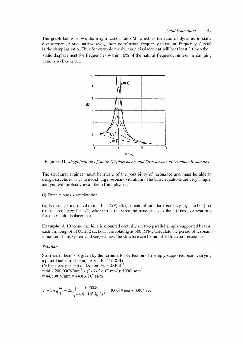
Load Estimation 49

The graph below shows the magnification ratio M, which is the ratio of dynamic to static displacement, plotted against �/�n, the ratio of actual frequency to natural frequency. �(zeta)

The structural engineer must be aware of the possibility of resonance and must be able to design structures so as to avoid large resonant vibrations. The basic equations are very simple, and you will probably recall them from physics: (i) Force = mass x acceleration (ii) Natural period of vibration T = 2��(m/k), or natural circular frequency �n = �(k/m), or natural frequency f = 1/T, where m is the vibrating mass and k is the stiffness, or restoring force per unit displacement. Example: A 10 tonne machine is mounted centrally on two parallel simply supported beams, each 3m long, of 310UB32 section. It is rotating at 600 RPM. Calculate the period of resonant vibration of this system and suggest how the structure can be modified to avoid resonance. Solution Stiffness of beams is given by the formula for deflection of a simply supported beam carrying a point load at mid span, i.e. y = PL3 / (48EI) Or k = force per unit deflection P/y = 48EI/L3 = 48 x 200,000N/mm2 x (2x63.2x106 mm4)/ 30003 mm3

= 44,800 N/mm = 44.8 x 106 N/m

26 /108.441000022

skgkg

kmT

��� �� = 0.0939 sec � 0.094 sec.

Figure 3.31 Magnification of Static Displacements and Stresses due to Dynamic Resonance

is the damping ratio. Thus for example the dynamic displacement will beat least 3 times the static displacement for frequencies within 10% of the natural frequency, unless the damping ratio is well over 0.1.

50 Load Estimation

Thus this machine will tend to experience problems with resonant vibration. Either the beams must be made stiffer, to increase the natural frequency, or less stiff to reduce it, or the structure must be modified in some other way, and/or damping must be introduced. Note that multiples of the natural frequency should also be avoided.

3.6.4 Vortex shedding When a fluid (e.g. air or water) flows past a bluff (i.e. not streamlined) body such as a building, a chimney, a bridge deck or a bridge pier, vortices are shed alternately on either side. If the frequency of vortex shedding corresponds to the natural frequency of a structure with little damping, dangerous vibrations may result. Vortex shedding caused the famous failure of the Tacoma Narrows suspension bridge in Washington. As shown above, natural frequencies of point masses on elastic beam type supports are easily calculated. When the mass is distributed along the elastic member it is not quite so simple. However you can get Spacegass to calculate it. Vortex shedding frequencies are also simple to calculate approximately from the following formula [5]: Frequency n = S Vo / d where S = Strouhal number = 0.2-0.3 approx (it varies to some extent with Reynolds number), Vo = flow velocity and d = diameter. Example: Calculate the vortex shedding frequency of flow past a 1 m diameter chimney if the wind velocity is 5 m/s. Solution

n = S Vo / d = 0.2 x 5/1 = 1 Hz There is one cycle of force causing oscillation in the direction of the wind for every vortex shed, and 1 cycle at right angles to the wind direction for every pair of vortices. Thus for the above example there would be 2 critical frequencies, 1 and 0.5 Hz.

wind

One oscillation cycle for every vortex shed

One oscillation cycle for every pair of vortices

Figure 3.26 Oscillations Induced by Vortex Shedding

Load Estimation 51

3.6.5 Worked Examples on Dynamic Loading

Example 3.6.5.1 Acceleration loads

A 1 tonne car rounds a 10 m radius bend on a roller coaster ride at 20 m/s. What radial load (1.5Q) must be designed for? (Centripetal acceleration a = v2/r). Solution

Force = ma = mv2/r = 1000 kg x (20 m/s)2 / 10 m = 40,000 N = 40 kN Example 3.6.5.2 Crane loads For an overhead crane with the details listed below calculate the factored design wheel load. Client requirements:

� Maximum safe lifted weight (SWL) = 150 kN � Crane rail AS41 � Crane span � portal frame span = 15 m � Intended purpose of crane: Frequent light loads, occasional loads near SWL � Required hoisting speed VH = 0.42 m/s Data supplied by crane manufacturer:� Crane frame self weight 80 kN (8 Ton) � Trolley (crab) + hook = 10 kN (1 Ton) � Maximum safe lifted weight (SWL) = 150 kN, Class 3 � Nearest approach of hook to rail (end carriage return) = 1 m � Wheel base SG or C = 2500 mm (wheel distance) � Load due to oblique travelling Pot = 13.8 kN � Lateral inertia loads Phb = 20.1 kN � Lateral inertia loads Phc = 1.8 kN � Longitudinal inertia Pht = 12 kN

Solution Static vertical loads

Maximum static vertical wheel reaction = PGH + PH where PGH = component of wheel load due to frame plus trolley, i.e. those parts that don’t move vertically

Crab

Crane Bridge

1 m 14 m

RA RB 80 kN7.5 m

10 kN

52 Load Estimation

PH = component of wheel load due to SWL carried by hook (ignoring weight of hook itself) i.e. the part that moves vertically. We will calculate these two components of the wheel reaction separately because we must apply and extra dynamic factor to the vertically moving load to account for upwards acceleration and braking while lowering the load. Looking at the crane in end elevation and taking moments about B, the “far side” rail, for the effect of parts that don’t move vertically:

15RA = 7.5 x 80 + 14 x 10 RA = 49.33 kN PGH = ½ RA (2 wheels) = 49.33 /2 = 24.67 kN Now for parts that do move vertically: 15RA = 14 x 150 RA = 140 kN PH = ½ RA = 70 kN

Dynamic magnification factors

Duty factor KD = 1.1 for class 3 cranes (this is applied to all moving loads, i.e. crane + hook load). Hoisting factor KH = 1.15 + 0.35VH where VH = hoisting speed in m/s

= 1.3 for this particular crane (applies only to SWL) Estimated maximum vertical wheel load = PGHKD + PHKDKH = 24.67x1.1 + 70x1.1x1.3 = 127.2 kNThis estimated actual load is treated as a live load Q on the runway beam, since it comes and goes. Thus the factored design vertical wheel load 1.5Q = 1.5 x 127.2 = 190.8 kN There will of course be 2 of these wheel loads on one rail, spaced 2500 mm apart in this case.

Lateral loads (horizontal loads at right angles to the runway beam) Pot

* = 1.5 x 13.8 = 20.7 kN Phb

* = 1.5 x 20.1 = 30.15 kN Phc

* = 1.5 x 1.8 = 2.7 kN

Longitudinal loads (parallel to the runway beam)

Pht* = 1.5 x 12 = 18 kN

This load will have very little effect on the crane runway beam but the bracing between the portal frames will have to be designed to withstand this load.

Load Estimation 53

Example 3.6.5.3 Unbalanced machines A machine weighing 20 tonnes is to be supported on a grid of 4 simply supported beams spanning 10 m. (i) Select a suitable beam section such that the maximum stress under static loading does

not exceed 100 MPa. (ii) Calculate the critical or resonant frequency of the system, treating the machine as a

point mass and ignoring the self weight of the beams. (iii) Suggest an alternative structure to increase the natural frequency. Solution Assuming each beam takes 20/4 = 5 tonnes = 5 x 9.8 = 49 kN as a point load at midspan, M* = PL / 4 = 49 x 10 / 4 = 122.5 kNm Max stress �max = M/Z � 100 MPa Elastic section modulus Z � 122.5x106 N mm / 100 N/mm2 = 1225x103 mm3 Select 460UB67.1 with Zx = 1300 x 103 mm3 Mid span deflection under static central point load y = PL3/48EI = 17.2 mm Stiffness of one beam k = P/y = 48EI/L3 = (48 x 200,000 N/mm2 x 296x106 mm4)/(10,000 mm)3 = 2842 N/mm = 2.84 x 106 N/m Natural period of vibration T = 2��(m/k) = 2��(5000kg/(2.84x106kg.m.s-2.m-1) = 0.263 sec

To increase the natural frequency we need to make the structure stiffer. We could do this be using two deeper beams with the required total Z � 4x1225 = 4900x103 mm3 For example two of 610UB101 would give almost the same Z (2x2530 = 5060x103 mm3 instead of 5200x103 mm3, but total I would increase from 4 x 296 = 1184x106 mm4 to 2x761 = 1522x106 mm4. This would increase stiffness a bit, but maybe not enough. (A single I section would not be stable, as it would not have enough torsional stiffness). Or we could go to 2 of 800WB122 (2 x 122 = 244 kg/m) without increasing weight and therefore at about the same cost as the original 4 of 460UB67.1 (4 x 67.1 = 268 kg/m). This would increase I to 2 x 1570 = 3140 x 106 mm4, increasing k by a ratio of 3140/1184 = 2.65, and hence natural frequency by a ratio of �2.65 = 1.63. This may be enough. If not, a much more effective way to increase stiffness drastically is to create a triangulated structure by adding diagonals, possibly as shown below, although this will depend on the particular situation.

Example 3.6.5.4 Vortex shedding A 1 m/s current flows past a series of jetty piers 0.4 m in diameter. Assuming S = 0.2, calculate the frequency of vortex shedding.

Solution Frequency n = S Vo / d = 0.2 x 1/ 0.4 = 0.5 Hz, i.e. period of 2 sec

54 Load Estimation

3.7 EARTHQUAKE LOADS

Earthquake loads are treated as a separate load category. However they are in fact a form of dynamic loading because they are caused by the acceleration of the ground, the inertia and the elastic behaviour of a structure. Earthquakes are of concern mainly with buildings of large mass and low ductility, e.g. unreinforced masonry, because large forces are needed to accelerate large masses and low ductility means there is little “give,” i.e. little capacity in the structure for energy absorption. Steel structures tend to be less susceptible to earthquakes than masonry buildings, but a steel framed structure such as a car park with heavy floor slabs and large live loads, or a structure supporting heavy machinery or other mass such as the tank stand, may be susceptible. Part 4 of the Australian loading code, AS1170.4[6], deals with earthquake loading. A brief introduction to earthquake load estimation is provided below. For a more comprehensive general introduction to the topic, the reader should study articles such as Hutchinson et al [7], which includes worked examples, and McBean [8], which discusses a specific example of an eccentrically braced frame.

3.7.1 Basic concepts

In order to start to understand how structures are affected by earthquakes, it is necessary to understand a few basic concepts. These are introduced below. 1. Ground acceleration. Earthquakes can cause movement in any direction with

accelerations up to about 0.2g or more. Early codes assumed an acceleration coefficient a = 0.1g = 0.98 m/s2. Thus a rigid building on a rigid foundation would be designed to resist a force F = ma = m approx. (note this is mass. not weight). So a building with a mass of 1000 kg would have a downward gravitational force of mg = 9.8 kN plus an earthquake load of approx 1 kN in any direction. Being only 10% of the gravity load its effects are negligible in the vertical direction, but they may be significant in any horizontal direction. So we must design for horizontal shear forces at each level depending on the mass of the structure above the level we are considering.

2. Periods of vibration. Various periods are present but as shown in the earthquake

accelerogram, Fig.4 of Hutchinson et al’s article[7], they are mainly much less than 1 sec. Since earthquakes contain most of their energy in the range of 1 to 10 Hz generally squat buildings don’t do well in an earthquake and tall buildings often do.

3. In the Australian code, AS 1170.4, horizontal shear forces are calculated from:

V = I(CS/Rf)Gg

where, V = total horizontal earthquake base shear. I = importance factor AS1170.4 Table 2.5

Load Estimation 55

C = earthquake design coefficient = 1.25a/T2/3 a = acceleration coefficient T = period of vibration of building = h / 46 approx, where h = height in m. S = site factor AS1170.4 Table 2.4(a) Rf = structural response factor AS1170.4 Table 6.2.6(a) Gg = gravity load (the weight G + �c Q above the plane considered) Codes allow for different acceleration coefficients in different regions depending on their history of seismic activity. Information in Australia is sketchy due to our short history, sparse population and relative geological stability - the contours in an area are often based on a single event - see for example Meckering in WA, which has a = 0.22, based on one event in the 1960s, and Tennant Creek in NT with a = 0.15 based on another event in the 1980s (see AS 1170.4, Figs.2.3 (a) and (e)). The Meckering and Tennant Creek earthquakes were major seismic events comparable in intensity to events which have killed thousands of people in more densely populated areas. They occurred in areas hitherto assumed to be seismically inactive and did little damage only because there was not much there to be damaged. They show that a major earthquake could hit anywhere anytime, and although the probability is low, the potential for loss of life and damage to infrastructure is high, so we need to take the possibility seriously.

3.7.2 Design procedure 1. Assuming it is not a structural alteration to an existing building and AS 1170.4 is

applicable (check Clause 1.1), decide if is a domestic structure (< 8.5 m high, < 16 m wide) or a general structure.

2. If a “general structure,” decide if it is “type III” (essential to post earthquake recovery). If so, importance factor I = 1.25, otherwise I = 1.

3. Determine acceleration coefficient “a” from map (ranging from 0.22 for Meckering, 0.15 Tennant Creek, 0.12 Bundaberg, down to 0.03 around Longreach and on the Nullarbor.

4. Determine period T = h / 46 approx, where h = height in m, for regular shaped buildings. 5. Hence earthquake design category from structure type, site factor and earthquake design

coefficient C = 1.25a/T2/3. 6. Calculate gravity load Gg = G + �cQ (see AS 1170.1) at each floor level. 7. Determine Site factor S from Table 2.4(a) or (b). S ranges from 0.67 (best) for a rock base

to 2 (worst) for loose sand to 12 m or more depth. 8. Determine Structural response factor Rf (Table 6.2.6(a) or (b)). This depends on how

brittle or ductile the structure is. It ranges from 8 (best) for special moment resisting frames of steel or reinforced concrete (e.g. eccentrically braced frames), through ordinary moment resisting frames of steel or reinforced concrete, down to 1.5 (worst) for unreinforced masonry shear walls.

9. Put them all together in V = I (CS/Rf) Gg to get shear force V. 10. Design building to take design shears at each storey level.

3.7.3 Worked Examples on Earthquake Load Estimation Example 3.7.3.1 Earthquake Loading on a Tank Stand

Calculate the earthquake loading on a steel tower used as a water tank stand. The tank stand has 4 legs of 100x100x6 EA, on a 3m square plan, 15 m high. Cross diagonal bracing is 50x50x5 EA at 45� in both directions. The tank is 5m in diameter, 2.4m high, weighing 5 kN empty. The tank stand is located in Bundaberg, take S = 1.

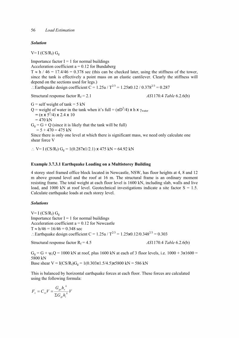
56 Load Estimation

Solution V= I (CS/Rf) Gg Importance factor I = 1 for normal buildings Acceleration coefficient a = 0.12 for Bundaberg T � h / 46 = 17.4/46 = 0.378 sec (this can be checked later, using the stiffness of the tower, since the tank is effectively a point mass on an elastic cantilever. Clearly the stiffness will depend on the sections used for legs.) Earthquake design coefficient C = 1.25a / T2/3 = 1.25x0.12 / 0.3782/3 = 0.287 Structural response factor Rf = 2.1 AS1170.4 Table 6.2.6(b) G = self weight of tank = 5 kN Q = weight of water in the tank when it’s full = (�D2/4) x h x �water = (� x 52/4) x 2.4 x 10 = 470 kN Gg = G + Q (since it is likely that the tank will be full) = 5 + 470 = 475 kN Since there is only one level at which there is significant mass, we need only calculate one shear force V

V= I (CS/Rf) Gg = 1(0.287x1/2.1) x 475 kN = 64.92 kN Example 3.7.3.1 Earthquake Loading on a Multistorey Building 4 storey steel framed office block located in Newcastle, NSW, has floor heights at 4, 8 and 12 m above ground level and the roof at 16 m. The structural frame is an ordinary moment resisting frame. The total weight at each floor level is 1600 kN, including slab, walls and live load, and 1000 kN at roof level. Geotechnical investigations indicate a site factor S = 1.5. Calculate earthquake loads at each storey level.

Solutions

V= I (CS/Rf) Gg Importance factor I = 1 for normal buildings Acceleration coefficient a = 0.12 for Newcastle T � h/46 = 16/46 = 0.348 sec Earthquake design coefficient C = 1.25a / T2/3 = 1.25x0.12/0.3482/3 = 0.303 Structural response factor Rf = 4.5 AS1170.4 Table 6.2.6(b) Gg = G + �cQ = 1000 kN at roof, plus 1600 kN at each of 3 floor levels, i.e. 1000 + 3x1600 = 5800 kN Base shear V = I(CS/Rf)Gg = 1(0.303x1.5/4.5)x5800 kN = 586 kN This is balanced by horizontal earthquake forces at each floor. These forces are calculated using the following formula:

VhG

hGVCF k

igi

kxgx

vxx�

��

Load Estimation 57

i.e. the force at each level = the base shear V times the coefficient Cvx for that floor. In this case, k = 1 since T < 0.5 sec. Thus the equation simplifies to:

VhG

hGVCF

igi

xgxvxx �

��

Cvx = (floor weight times height) divided by the sum of all (floor weight times height) (i.e. �Ggihi = 1600x4+1600x8+1600x12+1000x16 = 54400 kNm). The forces at each floor height are shown in the Table 3.2 Note that the cumulative shear Vx which the columns and bracing (if any) must withstand at each storey level is made up of the sum of the inertial earthquake forces acting on all floors above. This shear will cause bending moments in columns in a moment resisting frame (no diagonal bracing), or axial forces in a braced frame. The cumulative shear Vx will be shared between the two columns at the ground level Vx /col. = 586/2 = 293 kN The moment acting on each column at ground level Mx

* = 293 x 4 = 1172 kNm The moment Mx

* will cause tension in the windward columns and compression in leeward columns. Taking the free body diagram of the whole structure and then taking the summation of moment about any of the two base supports we can get the axial forces in the lower two columns. R x 8 = 69 x 4 + 138 x 8 + 207 x 12 + 172 x 16 R = 827 kN

Table 3.2

Storey Ggx(kN)

hx(m)

Cvx =Ggxhx / �Ggihi Fx (kN) Vx(kN)

Roof 1000 16 16000/54400 = 0.294 0.294x586= 172 172 3 1600 12 19200/54400 = 0.353 0.353x586 =207 379 2 1600 8 12800/54400 = 0.235 0.235x586 =138 517 1 1600 4 6400/54400 = 0.118 0.118x586 = 69 586

Ground - 0 - - 586 � 586

3.8 LOAD COMBINATIONS 3.8.1 Application

The purpose of load combinations is to obtain the most critical condition for which the structure must be designed.

3.8.2 Strength Design Load Combinations

The following load combinations must be considered when designing for strength (a) Dead load

1.35G

58 Load Estimation

(b) Live load (i) 1.2G + 1.5Q

(ii) 0.9G + 1.5Q (c) Wind load (i) 1.2G + Wu + �c Q

(ii) 0.9G + Wu (d) Earthquake (i) G + �c Q + Eu

(e) Snow, liquid pressure, earth pressure and ground water pressure (i) 1.2G + Su + �c Q

(ii) 0.9G + Su where Su is the snow load or liquid pressure or earth and/or ground water pressure.

3.8.3 Serviceability Design Load Combinations The following load combinations must be considered when designing for serviceability. (a) Short-term effects (i) G (ii) G + Ws (iii) G + �s Q (b) Long-term effects

(i) G (ii) G + �l Q �s, �l and �c, varies from 0.0 to 1.0 depending on the usage of the structure to be designed. the values for �c, �s and �l are given in Tables 3.3 and 3.4

Load Estimation 59

Table 3.3 Live Load Combination Factor for Strength Design

Type of Live Load Combination factor (�c)

Floors Domestic 0.4

Office 0.4 Parking area 0.4 Storage area 0.6

Other 0.6, unless otherwise assessed Roofs

Trafficable 0.4 Non-trafficable 0.0

Table 3.4 Live Load Factors for Serviceability Design

3.9 REFERENCES 1. Australian/New Zealand standard .AS/NZS 1170.1:2002 Permanent, imposed and

other actions. 2. Holmes, J.D. and Syme, M.J. (1994), Wind loads on Steel-Framed Low-Rise

Buildings. Steel Construction Vol.28, No.4, Dec., pp.2-12). 3. Australian/New Zealand standard. AS/NZS 1170.2:2002 Wind Actions. 4. Australian/New Zealand standard. AS/NZS 1170.3:2002 Snow and Ice Actions. 5. Roberson, J.A. and Crowe, C.T. (1997). Engineering Fluid Mechanics, Article 11.3). 6. Standards Association of Australia (1993). AS 1170.4 Earthquake Loads. 7. Hutchinson, G.L., Pham, L. and Wilson, J.L. (1994). Earthquake Resistant Design of

Steel Structures-an Introduction for the Practising engineer. Steel Construction, Vol.28 No.2 June, pp.6-22.

8. PC McBean. (1997). Steel Construction, Vol.31 No.1, March, pp.2-11.

Type of Live Load Short-term factor (�s ) Long-term factor (�l )

Floor Domestic 0.7 0.4 Offices 0.7 0.4

Parking area 0.7 0.4 Retail store 0.7 0.4

Storage 1.0 0.6 Other As for storage, unless otherwise assessed Roofs

Trafficable 0.7 0.4 Non-trafficable 0.7 0.0

60

4 METHODS OF STRUCTURAL ANALYSIS __________________________________________________________________________________

4.1 INTRODUCTION

Although analysis is an essential stage in design, some textbooks on the design of steel structures pay little attention to this stage. Textbooks on structural analysis, on the other hand, can be rather divorced from the practicalities of design. Section 4 of AS 4100[1] is entitled “methods of structural analysis,” and it contains some guidelines and rules, but on its own it is not enough to guide the designer through the analysis process. AS 4100 Supplement – 1999, the Steel Structures Commentary [2], contains further explanation and lists a large number of references on analysis. The present chapter does not attempt to duplicate existing references but provides some brief explanatory material including diagrams and examples where it is felt that these will help to clarify the provisions of AS 4100[1].

4.2 METHODS OF DETERMINING ACTION EFFECTS

AS 4100[1] Clause 4.1.1 refers to three methods of analysis: elastic, plastic and “advanced.” Most analysis is now done using commercial software packages such as Spacegass[3], Microstran[4] and Multiframe[5], using elastic methods, and this chapter will focus mainly on this approach, with a brief section on plastic analysis. Neither the code nor the commentary give any guidance as to how “advanced” analysis may be carried out. Clause 4.1.2 of AS 4100[1] defines braced members, in which transverse displacement of one end of the member relative to the other is prevented, and sway members, in which such displacement is allowed. Examples of braced members include all the members in a braced frame Fig.4.1 (b) and the horizontal members in a rectangular sway frame Fig.4.1 (a). Examples of sway members include the vertical members in a rectangular sway frame Fig.4.1 (a) and the columns and rafters in a pitched roof portal frame.

(a) Sway Frame (b) Braced Frame Figure 4.1 Sway and Braced Frame

Braced Member

Sway Member

Bracing Member

Methods of Structural Analysis 61

4.3 FORMS OF CONSTRUCTION ASSUMED FOR STRUCTURAL ANALYSIS Clause 4.2 of AS 4100[1] distinguishes between “rigid,” “semi-rigid” and “simple” construction. Most designers assume either rigid construction in which the angles between members do not change, or simple construction in which connections are assumed not to develop bending moments. Examples are shown in Fig.4.2. Semi-rigid construction, in which connections provide some flexural restraint but may not maintain original angles, may exist in reality but is more difficult to analyse and this analysis is usually avoided in practice.

(a) Rigid Rafter-Column Connection (b) Flexible Beam-Column Connection

Figure 4.2 Rigid and Flexible Connections

4.4 ASSUMPTIONS FOR ANALYSIS

Clause 4.3 deals with some assumptions that can be made to simplify structural analysis in some situations. For example the analysis of regular shaped structures with a large number of members can be simplified by treating sub-structures in isolation from the rest of the structure.

4.4.1 Treating sub-structures in isolation from the rest of the structure

For example the regular three-dimensional structure shown in Fig.4.3(a) below has 3 storeys, 4 bays in the X direction and 1 bay in the Z direction. According to Clause 4.3.1(a), this could be treated as a series of two-dimensional frames of 3 storeys and 4 bays in the x-y plane, and a series of two-dimensional frames of 3 storeys and 1 bay in the y-z plane as long as loads and stiffness do not vary markedly from one bay to another.

62 Methods of Structural Analysis

Figure 4.3(a) A Regular Building Structure treated as a Series of Parallel Two-

Dimensional Sub-Structures

Clause 4.3.1(b) deals with vertical loads on braced multi-storey building frames, in which a floor level plus the columns above and below can be treated as a sub-structure in isolation from the rest of the structure, as shown in Fig.4.3(b) below.

Braced three-dimensional structure with elements of substructure shown bold

A complete storey, comprising beams plus columns above and below,treated as an isolated substructure

Columns assumed fixed at levels above and below

A single beam considered as a substructure

Adjacent beams assumed fixed one span away

Figure 4.3(b) Assumptions for Individual Levels of Multi-Storey Buildings and Floor Beams

considered as Substructures

Methods of Structural Analysis 63

4.4.2 The effect of finite width of members

Structural analysis of skeletal structures treats structural members as "line elements," ignoring the fact that they actually have a finite width. Because of this finite width, it is usually impracticable to make connections at the centroid of each member. For example floor beams in simple construction multi-storey buildings must be joined to the sides of columns, and the weight supported by the beam does not act through the centroid of the column. The column must therefore carry not only axial force but bending moment also, as shown in Fig.4.3(c) below (unless there is another beam on the other side that exerts an equal and opposite moment on the column).They must therefore be designed as beam-columns, i.e. members under combined axial and bending loads, using Section 8 of AS 4100. Clause 4.3.2 of AS 4100 defines the span length as the centre to centre distance between supports, not the actual length of the beam, as shown in Fig.4.3(c) below. Clause 4.3.4 of AS4100 specifies the minimum eccentricity e of the load R from a simply supported beam acting on a column, as shown in Fig.4.3(c): “A beam reaction or a similar load on a column shall be taken as acting at a minimum distance of 100mm from the face of the column towards the span or at the centre of the bearing, whichever gives the greater eccentricity.”

Actual span

Assumed span (4.3.2)

Assumed line of action of load from beam acting on column: not less than 100 mm from face of column (4.3.4)

100 mm

Eccentricity e from column centreline

RR

Figure 4.3(c) Actual Span and Span Assumed in AS4100 The same clause also specifies the distribution of the resulting moment eR in the column as shown in Fig.4.3(d).

64 Methods of Structural Analysis

I2L2

I1L1 Lower ColumnI1L1

UpperColumnI2L2

Moment from eccentricity distributed in ratio of I1/L1 to I2/L2 and assumedto decrease to zero at floor levels above and below

UDL on beam

Figure 4.3(d) Distribution of Bending Moment from Eccentricity of Supports of Simply Supported Beam

Illustrative Example: Bending moments in columns due to eccentric vertical loads In the detail shown in Fig.4.3(e) below, the beam is simply supported on the angle, which is bolted to the face of the column. It is not clear exactly where the end reaction acts, so in accordance with Clause 4.3.4, it is taken as either the middle of the support (75 mm from column face) or 100 mm, whichever is greater, i.e. 100 mm.

Figure 4.3(e) A typical Beam-Column Connection showing Eccentricity of Load on Column

Beam carries 30 kN/m

6 m

150x150x12 EA

200UC46.2

Methods of Structural Analysis 65

To calculate the bending moment caused in the column by the eccentricity in the diagram above, 1. Calculate the total load on the beam as 30 kN/m x 6 m = 180 kN (ignoring the fact that 6

m is the distance between centres of columns and the actual beam length is a bit less. We will also assume the 30 kN/m includes the self-weight of the beam.

2. End reaction to support beam =180/2 = 90 kN. 3. Assume that this reaction force acts at a distance of 100 mm from the face of the column,

i.e. in this case 200 mm from the centreline of the column, since the column section is approximately 200 mm deep. Thus it will exert a moment of 90 kN x 0.2 m = 18 kNm. This moment must be balanced by moments in the columns above and below the connection.

4. Next the distribution factors between connecting members are calculated. Because a joint must be in equilibrium, the sum of the bending moments in the members connected at any joint must be zero (taking clockwise as positive and anticlockwise as negative). The 18 kNm moment exerted by the beam must be balanced by moments at the ends of the columns above and below, where they connect to the beam. For example if the storey height below is 4 m and that above is 3 m, the moments are distributed in the ratio 3 below to 4 above, i.e. the column below takes 18×3/7 = 7.7 kNm at the connection and the column below takes 18×4/7 = 10.3 kNm. These moments in the columns are assumed to decrease linearly to zero at the floor levels above and below, as shown in Fig.4.3(d). If there were another beam to the left of the column, the moment in it at this connection would also have to be taken into account.

4.5 ELASTIC ANALYSIS Most analysis of steel structures is done using elastic theory, although in practice some local yielding and plastic behavior is acceptable. Methods of analysis vary from approximate analysis using simplifying assumptions, through to highly sophisticated finite element analysis. Manual methods of analysis have now been largely replaced by faster and more accurate computer methods, but the designer should be aware of the existence of the older manual methods such as moment amplification and moment distribution. 4.5.1 First and second order elastic analysis

Clauses 4.4.1 and 4.4.2 of AS 4100 deal with first order analysis, in which deflections in members are not taken into account in calculating moments and forces, and second order analysis in which they are. Second order effects are illustrated in the examples below.

Illustrative Example 1:

A 6 m high signpost of 150x150x6 mm SHS section in Grade 350 steel carries a 50kN vertical load at an eccentricity of 0.5m, as shown in Fig.4.4(a). First order analysis predicts a uniform bending moment of 25 kNm, which corresponds to a maximum stress of 247 MPa, well below yield. The deflection at the top due to this uniform bending moment would be approximately 200mm.

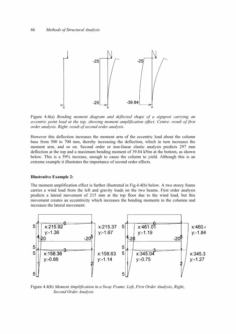
66 Methods of Structural Analysis

Figure 4.4(a) Bending moment diagram and deflected shape of a signpost carrying an eccentric point load at the top, showing moment amplification effect. Centre: result of first order analysis. Right: result of second order analysis. However this deflection increases the moment arm of the eccentric load about the column base from 500 to 700 mm, thereby increasing the deflection, which in turn increases the moment arm, and so on. Second order or non-linear elastic analysis predicts 297 mm deflection at the top and a maximum bending moment of 39.84 kNm at the bottom, as shown below. This is a 59% increase, enough to cause the column to yield. Although this is an extreme example it illustrates the importance of second order effects.

Illustrative Example 2:

The moment amplification effect is further illustrated in Fig.4.4(b) below. A two storey frame carries a wind load from the left and gravity loads on the two beams. First order analysis predicts a lateral movement of 215 mm at the top floor due to the wind load, but this movement creates an eccentricity which increases the bending moments in the columns and increases the lateral movement.

Figure 4.4(b) Moment Amplification in a Sway Frame: Left, First Order Analysis, Right, Second Order Analysis

Methods of Structural Analysis 67

4.5.2 Moment amplification

AS4100 provides equations for calculating moment amplification effects in braced members in Clause 4.4.2.2 and for sway members in Clause 4.4.2.3. These equations tend to give conservative predictions for normal cases and do not accurately predict extreme cases such as those shown above. They are intended for use as a part of a manual analysis process, but most analysis is now done using software packages which make the moment amplification equations obsolete. For a braced member subjected to axial compression, i.e. a member in a frame with diagonal bracing that effectively prevents sidesway such as a tankstand, clause 4.4.2.2 of AS4100 requires an increase in the design moment by a moment amplification factor �b which is given by:

11

*�

��

!""#

$%

�

omb

mb

NN

c� AS 4100 Cl. 4.4.2.2

where the factor cm = 0.6 – 0.4 �m � 1 allows a reduction in �b where the moment shape factor �m, given in Table 4.4.2.2, is favorable. N * is the design axial force and Nomb is the Euler buckling load for the axis of bending, i.e.normally the major or x axis (the code does not make this clear)

2

2

ecromb L

EPN &��

�

Illustrative Example 1: Moment Amplification Factor on a Braced Frame

An edge column in a building of “simple” construction is of 150UB14 section, effective length 4m. It has an axial compressive force N * = 50 kN and a uniform bending moment Mm* = 20 kNm calculated by first order analysis. Calculate �b and hence the amplified moment that should be used for design.

Solution

cm = 0.6 – 0.4 �m = 1.0 since �m = -1.0

8214000

1066.6000,2002

62

����

���

cromb PN kN

�b = 065.1

821501

1�

%

M * = �b Mm* = 1.065 x 20 = 21.3 kNm

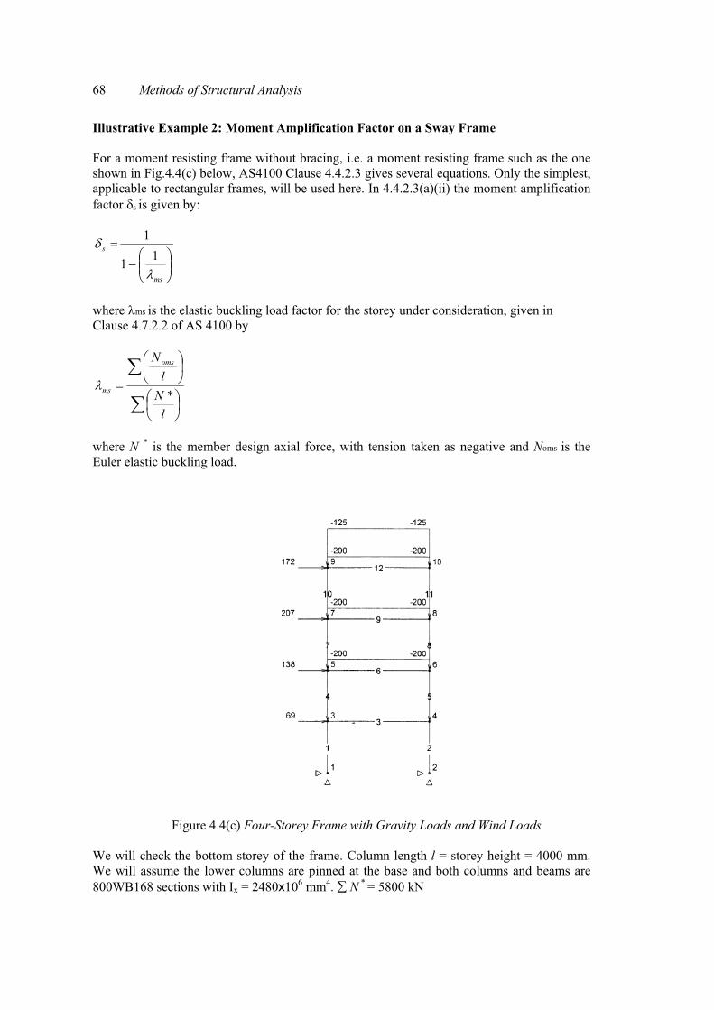
68 Methods of Structural Analysis

Illustrative Example 2: Moment Amplification Factor on a Sway Frame For a moment resisting frame without bracing, i.e. a moment resisting frame such as the one shown in Fig.4.4(c) below, AS4100 Clause 4.4.2.3 gives several equations. Only the simplest,applicable to rectangular frames, will be used here. In 4.4.2.3(a)(ii) the moment amplificationfactor �S is given by:

��

!""#

$%

�

ms

s

'

�11

1

where 'ms is the elastic buckling load factor for the storey under consideration, given in Clause 4.7.2.2 of AS 4100 by

�

�

� !

"#$

�

!"#

$

�

lNl

N oms

ms *'

where N * is the member design axial force, with tension taken as negative and Noms is the Euler elastic buckling load.

Figure 4.4(c) Four-Storey Frame with Gravity Loads and Wind Loads We will check the bottom storey of the frame. Column length l = storey height = 4000 mm. We will assume the lower columns are pinned at the base and both columns and beams are 800WB168 sections with Ix = 2480x106 mm4. � N * = 5800 kN

Methods of Structural Analysis 69

To calculate Noms we must estimate the effective length from AS 4100 Fig. 4.6.3.3(b). The stiffness ratio � is theoretically infinite for the pinned lower ends of the columns, i.e. the column is infinitely stiff compared to an ideal pin. However Clause 4.6.3.4(a) allows us to take �1 as 10 (taking the lower end as end 1). For �2 at the top of the columns we must calculate the ratio of stiffness of the columns to the beams joined at the top of the column under consideration:

�

�

� !

"#$ &

� !

"#$ &

�

be

c

l

l

��

where �e is determined from Table 4.6.3.4. In this case �e = 1 since the beam restraining the column under consideration is rigidly connected to a column at its other end. I is the same for the beam and the column, and l for the beam is 8 m, twice that for the column, so �2 = 2. To find the effective length factor ke we go up the left hand side of Fig.4.6.3.3(b) of AS4100 to �1 = 10 and across to �2 = 2. Thus ke = 2.15 and

( )2

2

lkEN

eoms

&�

� = 66189 kN

Hence

8.22

400058004000661892

�� !

"#$

� !

"#$ �

�ms'

Thus

046.1

8.2211

1�

� !

"#$%

�s�

i.e. we must increase the design moment by 4.6%.

Illustrative Example 3: Second Order Elastic Analysis of a Sway Frame It is just as easy to run a complete non-linear analysis using a computer package, if available, as it is to calculate 's manually. The results of first and second order analysis using Spacegass are shown in Fig.4.4(d) below. These show that the actual moment amplification on the bottom left hand column is 910/815 = 1.17, and the actual moment amplification on the bottom left hand column is 1620/1529 = 1.06. The latter figure is the important one, since both lower columns must be designed for the larger moment.

70 Methods of Structural Analysis

Figure 4.4(d) Bending Moments for Frame and Loads shown in Fig.4.4(c) Determined by First Order Analysis (left) and Second Order Analysis (right), using SpaceGass [3]

4.5.3 Moment distribution

This is a manual analysis process involving successive approximations, which was invented by Professor Hardy Cross in 1932. It was the normal method of analysing statically indeterminate frames before computers and analysis software became cheap and powerful enough to be generally available and practicable for use by practitioners. Moment distribution is very laborious for any but the simplest structures, but may still be useful when structural analysis software is not available.

4.5.4 Frame analysis software

Frame analysis software packages are now available that can analyse structural frames quickly and easily - provided the designer understands how to use them intelligently. Spacegass [3], Microstran [4] and Multiframe [5], are examples. There are also finite element analysis (FEA) packages, which can analyse and predict stresses and displacements in 2 or 3 dimensional continua. ANSYS [6] and STRAND [7] are examples. The present discussion is limited to frame analysis. Before using a frame analysis package the designer must understand the terminology and the way structures under load behave. The first thing to be aware of is that frame analysis packages treat structures as a series of lines of negligible thickness, joining nodes. For many types of structure this is quite accurate enough, provided allowance is made for eccentric forces as shown above. But structures such as walls, plates, shells and complex 3 dimensional shapes such as corbels require a more rigorous approach.

Methods of Structural Analysis 71

4.5.5 Finite element analysis Finite element analysis or FEA involves representing a real object as a “mesh” – a series of small, regularly shaped, connected elements, as shown in Fig.4.4(c), and then setting up and solving huge arrays of simultaneous equations. The finer the mesh of elements, the more accurate the results but the more computing power is required.

Figure 4.4(c) FEA Mesh and Stress Contours for a Box Girder Bridge

4.6 PLASTIC METHOD OF STRUCTURAL ANALYSIS

This is an alternative to the elastic method. Because it is not widely used it will not be treated in detail here. However the designer should be aware that it exists and know something of the principles involved. The basis of the method is that a ductile steel structure will not collapse as soon as yield occurs: one or more “plastic hinges” must form. Plastic hinges are sections where the full section has reached the yield stress. Once the plastic moment has been reached it is assumed that the section can offer no additional resistance to rotation, behaving as a hinge but with constant resistance Mp, a condition known as a plastic hinge (in fact there will be a slight increase in moment due to strain hardening as the rotation at a plastic hinge increases). In general, any combination of three hinges, real or plastic, in a span will create an unstable situation known as a collapse mechanism. Because we design structures to survive extreme loads, it makes sense to examine what loading will cause actual collapse of a structure, and then apply suitable load factors to ensure that we have an acceptable margin of safety before collapse. Thus for example a simply supported beam with a point load at midspan or a UDL (uniformly distributed load) will collapse when one plastic hinge forms at midspan. The “plastic moment” Mp, i.e. the moment necessary to form a plastic hinge, is given by: Mp = fy S

72 Methods of Structural Analysis where fy = yield stress, and S = plastic section modulus (listed in tables of section dimensions and properties. Note that in Australia Z = elastic section modulus and S = plastic section modulus. In the USA the reverse notation is used. The elastic and plastic section modulus for built up sections with one axis of symmetry can be calculated using the principles of stress analysis. Illustrative Example 1:

Find the yield moment My and the plastic moment Mp for a 610UB125 section of Grade 300 steel. Hence find the UDL w (in kN/m) on a simply supported beam of this section, spanning 16m, that would cause (a) first yield, (b) collapse.

Solution My = fy Z = 300 x 3230 x 103

= 969 kNm Mp = fy S = 300 x 3680 x 103

= 1104 kNm (a) for first yield and including the capacity factor �

�My =8

2Lwy

���

� 2169699.08

yw 27.25 kN/m

(b) for collapse and including the capacity factor �

�Mp =8

2Lwc

���

� 21611049.08

cw 31.05 kN/m, which is 14% higher than the UDL for first yield.

A beam with fixed ends will require three plastic hinges, one at midspan and one at each end, before it will collapse. For a fixed end beam with a point load at midspan, the midspan moment = end moments = PL/8 = half the midspan moment for a simply supported beam. Thus the fixed end beam can take double the load before first yield, and yield will occur simultaneously at all 3 potential plastic hinge points. However for a UDL, the end moments are wL2/12, double the midspan moment, so as the load increases, yield will occur first at the ends. Once plastic hinges form at the ends, the ends will rotate so the beam behaves as if the ends are partially fixed, and the midspan moment increases until yield occurs there, and finally a plastic hinge, at which point the beam collapses.

Illustrative Example 2:

Find the UDL w (in kN/m) on a fixed end beam of Grade 300, 610UB125 section, spanning 16m, that would cause (a) first yield (b) collapse.

Solution

As in the example above, My = 969 kNm Mp = 1104 kNm