Embed Size (px)
Citation preview

Steady State Performance of an Elastic Flexible
Wing
by
William Edward Gorgen
B.S., Massachusetts Institute of Technology (1991)
Submitted to the Department of Aeronautics and Astronautics
in partial fulfillment of the requirements for the degree of
Master of Science in Aeronautics and Astronautics
at the
MASSACHUSETTS INSTITUTE OF TECHNOLOGY
May 1993
© Massachusetts Institute of Technology 1993. All rights reserved.
Author ..................... ...........
Department of Aeronautics and AstronauticsMay 18, 1993
Certified by.Sheila E. Widnall
Professor of Aeronautics and AstronauticsThesis Supervisor
Accepted by ..... ....... {/ ......................................Professor Harold Y. Wachman
Chairman, Departmental Graduate Committee
MASSACHUSETTS INSTITUTE(Wr Tcrijsfl' nav
'JUN 08 1993LISRAH kI
C..~G"' ~~"

Steady State Performance of an Elastic Flexible Wing
by
William Edward Gorgen
Submitted to the Department of Aeronautics and Astronauticson May 18, 1993, in partial fulfillment of the
requirements for the degree ofMaster of Science in Aeronautics and Astronautics
Abstract
This Study considers a flexible wing which is designed to change camber in re-sponse to lift loads. This cambering response is achieved by properly constraininga flexible bending plate-like wing. By supporting the leading and trailing edges ofsuch a wing, the lift loads cause the wing to camber. The performance of flexiblewings differs significantly from traditional rigid wings. The variable camber of theflexible wings results in a lift curve whose slope depends on the stiffness of the airfoilas related to the dynamic pressure of the flow. This relative stiffness of the bendingplate to the dynamic pressure of the flow is measured by a non-dimensional stiffnessparameter. A numerical analysis combining a vortex lattice aerodynamic model anda finite element structural model is used to determine the performance characteristicsof these wings. The analysis is idealized by including only the linear bending effects ofthe structure and the inviscid aerodynamics of the wing. The results of the analysisshow the theoretical performance characteristics of flexible wings in terms of the liftcurve slope of the wing as related to its stiffness and aspect ratio.
Thesis Supervisor: Sheila E. WidnallTitle: Professor of Aeronautics and Astronautics

Acknowledgments
I would like to thank all of the people who helped me through MIT and helped mefinish my thesis. I have been very fortunate during the past few years to have had anopportunity to participate in several exiting projects. Without the many people thatwere involved in these projects, I would not have learned as much or had as muchfun. I would like to thank all of the people for all that they have meant to me overthe years.
I could have never done any of this work without the help and friendship ofJeff "Orville" Evernham. Together, we conceived of a flexibly cambering wing andsought to develop it as a sailboard fin for our own boards. Without his input andcollaboration, the entire concept would not exist. Of course, without Jeff's unendingenthusiasm for the sport of windsurfing, I would still be practicing my waterstarts ona transition board. And without his companionship in the classroom and at ThetaXi, I surely would have never been able to finish even a single degree in aeronauticalengineering, much less two. But most of all, I want to thank Jeff for all the crazinessand fun that we had together.
During the past two years, it could have been easy for me to fall into a dailyregimen of studies and work. And without the constant encouragement from MattButler, Ted Liefield, Scott Stephenson, Rick "Pax" Paxson and the rest of the gang, Ijust may have. Thanks guys for keeping me swimming in beer at crucial times in mygraduate career. And thanks as well to the bands Letters To Cleo, Cliffs of Dooneenand Chucklehead for making the nights at the clubs such memorable events.
The times away from school added so much to the years I've spent here. I'd liketo thank The Boyz (and Girlz) of BL)A and our sister sorority, IIME, for all the funand crazy times. Living with them was never dull.
I'd also like to thank Alex Chisholm. Alex gave me a unique perspective on theworld and taught me more about life than he will ever know. The time I spentwith Alex is some of the most memorable and important times of my college career.Without Alex, I would have never survived emotionally.
My family was always there for me and supported me throughout my college life.My dad, as an engineer, could understand many of the issues I faced and encouragedme to keep working. My mom, who kept asking if I had finished my "paper", sup-ported me in more ways that I can express. My sister Mary kept me sane for thesepast years by keeping my social skills up to date. The rest of my family also gave mesupport and encouragement in all of my endeavors.

I'd like to thank Sheila and Bill Widnall who believed in the idea of flexiblewings enough to support my work not only in graduate school, but also in Flex FoilTechnology Corporation which they co-founded with Jeff Evernham and I. If it wasnot for sheila's guidance on the development of this idea, it would probably havenever gotten off the ground.
I'd also like to thank Prof. Mark Drela for teaching me how to design wings. Hisinspired teaching as well as his guidance of the Decavitator Hydrofiol Team inspiredme to dream of flight in all of its forms. Mark also taught me that fluid dynamicsoften can be studied with a pint or two of one of Cambridge Brewery's Ales.
Developing numerical algorithms to solve problem can often be a tedious program-ming task. However, it can be impossible without the support of people who havedone similar work before. Without Steve Ellis, the Athena God who kept Reynoldsand the rest of the Fluid Dynamics Research Lab's Computer hardware up and run-ning, I never could have finished my research. I'd also like to thank Harold "Guppy"Youngren for giving me his vortex lattice code and advice on how to use it and modifyit. Prof. Mike Graves who taught me all about the inner workings of Finite Elementprograms. Prof. Bathe from the Mechanical Engineering department answered anendless barrage of questions from me about how to make his ADINA program work.And I'd also like to thank the Freindly people at the MITSF who put up with mystupidity on the cray.
In trying to turn all of my ideas into reality, I spent a lot of time in the Aero-AstroProjects lab building models. I'd like to thank Jeff DiTullio, Dick Perdichizzi, DonWeiner and Earle Wassmouth who let me run wild in their machine shop. Thanksespecially to Jeff, who was an unlimited pool of information about composite produc-tion techniques.
Finally, I'd like to thank all of my officemates for making the office such a greatplace to work. I wish all of them the best of luck with their reseach as well. Hopefullythey will have as much fun as I did.

Contents
1 Introduction
1.1 Description of Flexible Wings . . . . . . . .
1.2 Advantages of Flexible Wings . . . . . . . .
1.3 Applications ............ . . .....
1.3.1 Aircraft .. .. .. ... .. .. .. .
1.3.2 Sailcraft Keels and Sails .......
1.3.3 Turbomachinery ..... .......
2 Theory and and Modeling of Flexible Wings
2.1 Classical Theories . . . . . . . . . . . . . . .
2.1.1 Two-Dimensional Plate Theory . . .
2.1.2 Airfoil Theory .............
2.2 Elastic Airfoil Theory . . . . . . . . . . . . .
2.2.1 Linear Theory of Flexible Airfoils . .
2.2.2 Stiffness Parameter . . . . . . . . . .
2.2.3 Critical Stiffness . . . . . . . . . . .
2.2.4 Effect of Spar Placement . . . . . . .
2.3 Two-Dimensional XFOIL Tests . . . . . . .
2.4 Three-Dimensional Extension . . . . . . . . .
2.4.1 Flexible Wings of Finite Span .....
2.4.2 Effective Stiffness . . . . . . . . . . . .
3 Numerical Methodology
20
20
21
23
25
26
27
28
29
31
34
37
38
. . . . . . . . . . .
. . . . . . . . . . .

3.1 Vortex Lattice Aerodynamic Model . . .
3.1.1 Geometry .............
3.1.2 Formulation of the Vortex Lattice
3.1.3 Determination of vortex strength
3.1.4 Solution and Discrete Forces . . .
3.1.5 Total Forces and Non-Dimensional
3.1.6 Trefftz Plane Drag Calculation .
3.1.7 Vortex Lattice Program Overview
3.2 Finite Element Model ...........
3.2.1 Formulation of the Finite Element
3.2.2 Local Element Coordinate System
3.2.3 Element Stiffness Matrix.....
3.2.4 Global Stiffness Matrix......
3.2.5 Solution Method .........
3.2.6 ADINA program overview . . . .
3.3 Interaction of Numerical Programs .
3.3.1 Geometric Relationship . . . . . .
3.3.2 VL: Lift Load Information . . . .
3.3.3 FEM: Displacements . . . . . . .
3.3.4 Iteration of Solution . . . . . . .
Force
Mesh
Coefficients
. . . .. ,
3.3.5 Special considerations for a flexible wing
4 Numerical Analysis of Flexible Wings
4.1 Analysis Goals ...................
4.1.1 Convergence .................
4.1.2 Parameter Range . . . . . . . . . . . . . .
4.1.3 Data and Results ..............
4.2 Verification Tests ..................
4.2.1 Rectangular Planform . . . . . . . . . . .
4.2.2 Convergence Tests . . . . . . . . . . . . .
4.2.3 Linearity of Lift Curve ............
4.2.4 Numerical Results ..............
4.2.5 Drag Polar ...................
4.3 Analysis of Ideal Tapered Wings ...........
4.3.1 Tapered Wing Planforms ...........
4.3.2 Numerical Convergence of Tapered Planform
4.3.3 Linearity of Lift Curve ............
4.3.4 Induced Drag Polars .............
4.3.5 Stiffness Effect on Lift Curve Slope . . . . .
4.3.6 Aspect Ratio Effect on Flexible Wings . . .
4.3.7 Lift Performance Of Ideal Tapered Wings
4.4 Analysis of Non-Ideal Tapered Wings . . . . . . . .
4.4.1 Spar Boundary Conditions ..........
4.4.2 Non-Uniform Plate Stiffness . . . . . . . . .
4.5 Tests Involving Sailboard Fin Planforms . . . . . .
4.5.1 Sailboard Fin Planforms ...........
4.5.2 Convergence Tests ..............
4.5.3 Linearity of Lift Curve ............
4.5.4 Performance of 8 Inch Flex Foil Wing . .
4.5.5 Performance of 10 Inch Flex Foil Wing . . .
4.5.6 Critical Speed for 10 inch Fin . . . . . . . .
5 Conclusions and Recommendations
5.1 Performance Characteristics of Flexible Wings . . .
5.1.1 Camber Stability ...............
5.1.2 Lift Performance ...............
5.1.3 Angle of Attack ................
5.1.4
5.1.5
5.1.6
Variation of Parameters with Planform Type .
Low Aspect Ratio Performance . . . . . . . .
Drag Performance ................
. . . . . . . . . . 68
.. .. ... ... 72
. ... ... ... 73
. ... ... ... 75
. ... .... .. 75
S . . . . . . . . . 78
.. ... ... .. 79
.. ... ... .. 80
S . . . . . . . . . 80
S . . . . . . . . . 82
S . . . . . . . . . 85
S . . . . . . . . . 85
.. .... .. .. 85
S . . . . . . . . . 90
S . . . . . . . . . 94
.. .... .. .. 94
... ... .. .. 97
... ... .. .. 97
S . . . . . . . . 99
S . . . . . . . . . 100
S . . . . . . . . . 101
102
S . . . . . . . . 102
... ... ... 102
. .. ... ... 103
. .. ... ... 104
S . . . . . . . . 105
S . . . . . . . . 105
. .. .... .. 106

5.2 Design of Flexible W ings ......................... 108
5.2.1 Steady Load Lifting Surfaces. ..... ............. . 108
5.2.2 Control Surfaces ......................... 109
5.3 Recommendations for Further Study . ................. 110
5.3.1 Spar Placement .......................... 110
5.3.2 Viscous Drag ........................ ... 111
5.3.3 Planforms .......................... ... 111
5.3.4 Non-Uniform Stiffness in the Spanwise Direction ........ 111
5.3.5 Other Non-Uniform Chordwise Stiffness Distributions ..... . 111
5.3.6 W ind Tunnel Tests ........................ 112
5.3.7 Shred . . . . . . . . . . . . . . . . . . . . . . . . . . . . . . . 112
A Effective Stiffness Analysis 113
A.1 Two-Dimensional Effective Stiffness Tests . ............... 113
A.1.1 Plate with Ideal Boundary Conditions . ............ 114
A.1.2 Plate with Spar B.C.s and Uniform Thickness . ........ 116
A.1.3 Plate with Spar B.C.s and NACA Thickness . ......... 119
A.1.4 Determination of Airfoil Critical Stiffness . ........... 121
A.2 Tapered W ing ............................... 121
A.2.1 Ideal Boundary Conditions ................... . 122
A.2.2 Spar B.C.s and Uniform Thickness . .............. 124
A.2.3 Spar B.C.s and NACA Thickness . ............... 126
A.3 Flexible Sailboard Fins .......................... 128
A.3.1 8 inch Flex Foil Fin Planform . ................. 128
A.3.2 10 inch Flex Foil Fin Planform . ................ 131
B Numerical Analysis 133
B.1 Tapered Wing: Ideal Boundary Conditions . .............. 133
B.2 Aspect Ratio 5 Tapered Wing: Spar Boundary Conditions ...... 136
B.2.1 Aspect Ratio 5 Tapered Wing: Uniform Thickness ....... 136
B.2.2 Aspect Ratio 5 Wing: NACA Thickness . ........... 137

B.3 Flexible Sailboard Fins .......................... 140
B.3.1 8 inch Fin Planform ....................... 140
B.3.2 10 Inch Fin Planforms ...................... 140

List of Figures
2-1 Simply Supported Plate Acted on by a Distributed Load . . . . . . .
2-2
2-3
2-4
2-5
2-6
2-7
2-8
2-9
2-10
3-1
3-2
3-3
3-4
3-5
4-1
4-2
4-3
4-4
4-5
4-6
4-7
Lift Curves for a Flexible Airfoil and Rigid Airfoils of Various Camber
Lift Curves for Airfoils of Various K Values . . . . . . . . . . . . . . .
Drag Polars for Airfoils of Various Cambers . . . . . . . . . . . . . .
XFOIL Results: Lift curves for Viscous Airfoils . . . . . . . . . . . .
XFOIL Results: Drag Polars for Viscous Airfoils . . . . . . . . . . . .
Lift curve for a Finite Wing .......................
Elliptic Lift Distribution for a Finite Wing . . . . . . . . . . . . . . .
Lift Curve Slopes of Tapered and Elliptic Planforms . . . . . . . . . .
Effective Stiffness Test Setup .......................
Vortex Lattice Geometrical Representation . . . . . . . . . . . . . . .
Trefftz Plane Intersecting Wake Vortex Sheet . . . . . . . . . . . . . .
Nodal d.o.f.s . . .. .. .. ... .. .. .. .. ... . . . . .. . . . .
Triangular Area Coordinates .......................
Overlay of Finite Element Mesh and Vortex Lattice . . . . . . . . . .
Verification Test: Convergence Rate . . . . . . . . . . . . . . . . . . .
Verification Test: Angle of Attack Convergence . . . . . . . . . . . .
Linearity of Lift Curves for Rectangular Planform . . . . . . . . . . .
Stiffness Effects on Lift Curves Slope for Rectangular Planform . . .
Induced Drag Polar for Rectangular Planform . . . . . . . . . . . . .
Typical Tapered Flexible Wing Model . . . . . . . . . . . . . . . . .
Lift Curve Slopes for Tapered Planforms of Various Aspect Ratio . .

4-8 Convergence Rate for Tapered Planform . .......... . . . . . 78
4-9 Convergence Rate for Tapered Planform . ............ . . . 79
4-10 Linearity of Lift Curves for Tapered Planform . ............ 80
4-11 Similarity of Drag Polars for Tapered Planform . ........... 81
4-12 Lift Curve Slope as a Function of Stiffness . .............. 82
4-13 Aspect Ratio Effects on Critical Stiffness . ............ . . . 83
4-14 Proportionality Coefficient for ideal Tapered Planform . ....... 84
4-15 Stiffness Parameter Affect on Lift Curve Slope . ............ 88
4-16 Aspect Ratio effect on F ......................... 89
4-17 Aspect Ratio Effects on Critical Stiffness for Wing with Spars . . .. 90
4-18 Comparison of Uniform and Non-Uniform Thickness Wings ...... 92
4-19 Effect of Non-Uniform Thickness on Critical Stiffness . ........ 93
4-20 Effect of Non-Uniform Thickness on Proportionality Coefficient, F . 94
4-21 Typical Flexible Sailboard Fin Model . ................. 96
4-22 Convergence Rate ........................... 97
4-23 Linearity of Lift Curves for the 8 inch Flex Foil Planform ...... . 98
4-24 Performance Curve for 8 inch Flex Foil Planform . .......... 99
4-25 Performance Curve for 10 inch Flex Foil Planform . .......... 100
4-26 Critical Speed for 10 inch Flex Foil Planform . .......... . 101
A-1 Effective Stiffness Test: Ideal B.C.s . .................. 115
A-2 Effective Stiffness Test: Ideal B.C.s . .................. 116
A-3 Effective Stiffness Test: Spar B.C.s and Uniform Thickness ...... 117
A-4 Effective Stiffness Test: Spar B.C.s and Uniform Thickness ...... 118
A-5 Effective Stiffness Test: Spar B.C.s with NACA Thickness ...... 119
A-6 Effective Stiffness Test: Spar B.C.s and NACA Thickness ....... 120
A-7 Ideal Tapered Wing: Effective Stiffness Test Loading . ........ 122
A-8 Ideal Tapered Wing: Effective Stiffness Test Deflection . ....... 123
A-9 Ideal Tapered Wing: Effective Stiffness Test Loading . ........ 124
A-10 Ideal Tapered Wing: Effective Stiffness Test Deflection . ....... 125

A-11 NACA Tapered Wing: Effective Stiffness Test Load ......... . 126
A-12 NACA Tapered Wing: Effective Stiffness Test Deflection ...... . 127
A-13 8 inch Flex Foil Fin: Effective Stiffness Test Load . .......... 129
A-14 8 inch Flex Foil Fin: Effective Stiffness Test Deflection . ....... 130
A-15 10 inch Flex Foil Fin: Effective Stiffness Test Load . ......... 131
A-16 10 inch Flex Foil Fin: Effective Stiffness Test Deflection ........ 132
B-1 AR 5 Tapered Flexible Wing: Rigid Loading . ............. 134
B-2 Ideal AR 5 Flexible Wing: Load at Kcrit . ............ . . . 134
B-3 Ideal AR 5 Flexible Wing: Camber at Kcrit . .......... . . . 135
B-4 Uniform thickness AR 5 Flexible Wing: Load at Kcrit ......... 136
B-5 Uniform Thickness AR 5 Flexible Wing: Camber at Kcrit ....... 137
B-6 NACA AR 5 Flexible Wing: Load at Kcrit . .............. 138
B-7 NACA AR 5 Flexible Wing: Camber at Kcrit . ............ 139
B-8 8 inch Flex Foil Planform: Initial Load . ................ 140
B-9 8 inch Flex Foil Planform: Load at Kcrit . ............... 141
B-10 8 inch Flex Foil Planform: Camber at Kcrit . ............. 142
B-11 10 inch Flex Foil Planform: Initial Load . ............... 143
B-12 10 inch Flex Foil Planform: Load at Kcrit . .............. 144
B-13 10 inch Flex Foil Planform: Camber at Kcrit . ............. 145

List of Tables
4.1 Correlation Coefficients for Rectangular Planform . .......... 71
4.2 Correlation Coefficients for Tapered Planform . ............ 79
4.3 Correlation Coefficients for 8 inch Flex Foil Planform . ........ 98
A.1 2-D Critical Stiffness Calculations . .................. . 121

Chapter 1
Introduction
One of the main goals in the design of a lifting body such as a wing is to maximize
the lift to drag ratio. This desire to minimize drag resulted in the development of
cambered airfoil sections for wings. Adding camber to wings has the effect of increas-
ing the amount of lift that can be achieved at a certain angle of attack. Camber
also increases the magnitude of the lift that can be generated before the wing transi-
tions from low drag laminar flow to high drag turbulent flow. By properly designing
the camber of a wing it is possible to achieve a high lift to drag ratio for a certain
range of operating points. Traditional fixed geometry wings generate lift through a
combination of camber and angle of attack. However, since the amount of camber
is fixed, these wings can only increase the amount of lift they are generating by in-
creasing their angle of attack. This tends to add drag and decreases the efficiency of
the wings. Thus, the range of efficient operation of a fixed-camber wing is limited to
a small range close to the operating point that it was designed for. When the wings
deviate too far from this design point, their efficiency goes down.
By utilizing airfoil sections that change camber as the operating point changes, it
is possible to extend that range of efficient operation of a wing. Wings of this type
are known as variable geometry wings. The characteristics of these wings make them
ideal for vehicles that require a large range of lifting needs, a wide range of speeds or a
need to generate both positive and negative lift. There are many wing designs which
utilize variable geometry airfoils but their shapes are usually controlled externally by
the use of mechanical actuators that deploy leading edge flaps or slats or otherwise
change the shape of the wing. While these wings often achieve significant performance
advantages over fixed geometry wings, the control and actuation system is often too
large and complex to be practical for many smaller applications.
An elastically flexible wing changes its camber shape automatically, in response to
lifting loads. Such an automatic camber-adjusting wing does not use external control
devices to change camber, but rather controls the shape through the elastic flexibility
of the chordline. Because this wing can change its amount of camber, it responds to
an increased lift requirement by increasing its camber as well as its angle of attack.
This automatic cambering behavior in response to load is achieved by controlling
the flexibility of the wing in the chordwise direction. By having a flexible chordline
and being constrained in deflection at the leading and trailing edges, the lift forces
push up on the center of the wing and bend it into a cambered shape. Thus, additional
lift is generated by an increase in camber as well as a change in angle of attack. This
increase in camber allows the wing to generate the increased lift more efficiently.
1.1 Description of Flexible Wings
The elastically flexible wings considered in this work are comprised of a flexible
plate in the shape of a wing with an aerodynamic thickness distribution. The plate
is supported by explicitly prescribed boundary conditions at the leading and trailing
edges of the wing or by rigid spars along the leading and trailing edges that are
cantilevered at the root of the wing. The spars are mounted to the craft such that
they are free to pivot around their major axes. The spar that runs along the trailing
edge is also free to slide in the chordwise direction to provide simple support to the
plate. Thus, the spars constrain the deflection of the wing under load such that the
wing is reasonably flexible in the chordwise direction but is not allowed to deform in
the spanwise direction providing a flexible camberline.
By properly constraining the leading and trailing edge deflections, the wing can
be made to increase its camber as the lift loads increase. By the proper tailoring of

the flexibility of the camberline, the wing can increase its camber in direct proportion
to the lift loads. The flexible region should be flexible enough so that the lift loads
cause it to camber, but not so flexible that it cambers more than desired.
1.2 Advantages of Flexible Wings
Flexible wings have many advantages over standard fixed geometry wings. Rigid
wings are designed to operate mainly at one operating point. The camber of these
wings is designed to maximize the performance at that point. Wings operating at
low lift coefficients generally have low camber while higher lift coefficients generally
demand higher camber. Due to their ability to change camber, flexible wings have
a much broader range of lift loads where they can operate efficiently. At low lift,
these wings have only a small amount of camber much like the rigid wing designed to
operate at that same operating point. However, at higher lift, the camber is increased
and thus the wing operates like the rigid wing with higher camber. Thus, the flexible
wing has the ability to perform with high efficiency over a much broader range of
operating points than any one fixed geometry wing.
A flexible wing also resists stalling. Most rigid wings are designed to operate at a
moderate lift point. The camber of the wing is designed to optimize the performance
of the wing at that point. When such a wing is operated at a much higher lift point,
it is prone to stall since it does not have enough camber for that amount of lift and
must drastically increase its angle of attack. For a flexible wing, an increased lift
need is met by a camber increase as well as an increase in angle of attack. Thus, the
increase in angle of attack is less for the flexible wing than it is for the rigid wing and
the flexible wing is further from its stall point.
1.3 Applications
Flexible wings are particularly well suited for certain applications. Given their
ability to camber in the direction of the lift force, they work well on lifting bodies

that may need to generate lift in either directions such as lifting surfaces on sailboats
or control surfaces on aircraft. They may also work well for devices that have a large
range of lift requirements such as compressor or turbine blades in turbomachinery.
1.3.1 Aircraft
There are many types of aircraft that could utilize a wing with a wide performance
range. It is not uncommon for an aerobatic aircraft to perform maneuvers that can
require the wings to operate anywhere between +6g and -2g or more. The wings of
such aircraft would need to be able to generate lift up to 6 times the weight of the
aircraft as well as negative lift of 2 times the weight of the aircraft. Standard fixed
geometry wings are often pushed to their aerodynamic limit, or stall point, by such
extreme maneuvers. A flexible wing would be much further from its limit at these
points and would be in a more efficient configuration than the fixed geometry wings.
This would give the aerobatic plane a much greater stall margin as well as reduced
drag, and thus more speed, through the maneuvers.
These flexible wings could also be used for control surfaces on aircraft with more
conservative operation. The elevators and rudders on such aircraft operate through a
wide range of lift needs. A flexible wing could adjust its camber to remain in a efficient
configuration throughout a wide range of lift points giving an efficient configuration
for a wide range of control surface positions.
1.3.2 Sailcraft Keels and Sails
Sailcraft have a unique place in the world of fluid dynamics. The sails and un-
derwater appendages (such as rudders and keels) of sailcraft need to generate lift in
either direction depending on the direction they are sailing in. In some operating
points the wind blows over the port side of the craft and in other operating points
the wind blows over the starboard side of the craft. Thus on some points of sail
the lifting bodies must generate lift in one direction and on other points of sail the
pressure and suction surfaces are reversed. This unique need to generate lift in both

directions resulted in the development of sails that can camber from side to side as
the wind pushes on them.
However, traditional sails behave in a very different way than the flexible wings
studied here. Structurally, a wing is a membrane rather than a bending plate. The
deflection state of the loaded membrane is determined by the tensions that build up
in the membrane rather than the bending strains that are associated with the plate.
The shape of a sail is determined mainly by the way that the sailmaker cut the cloth
of the sail. The sail tends to exhibit a "snap through" camber response where it takes
on one of only two possible shapes; positively cambered or negatively cambered. The
shape of the elastic flexible wing studied is proportional to the loading on it.
In a similar way, a flexible wing can camber in either direction depending on the
direction of the lift forces. By having a flexible wing for a keel, the drag of the
craft can be reduced and the craft can go faster. The ability to camber in either
direction allows the performance advantages to be realized on either tack. The elastic
response of the camber to the lift allows the keel to adjust to the lift need of the boat.
Flexible wings can also give rudders better control authority. The rudder, much like
the elevators on aircraft, needs to generate lift in either direction to quickly adjust
the direction of the boat. A flexible rudder could reduce the drag associated with the
steering the boat allowing the boat to maintain more speed through maneuvers.
1.3.3 Turbomachinery
The compressors in turbomachinery act to push air or some other fluid through
the turbomachine. The turbines of these machines act to extract energy from the
fluid. Both the compressors and turbines make use of lifting bodies to impart or
extract energy from the fluid flow. In many applications, these lifting bodies are
blades with airfoil cross-sections. The performance of these blades is limited by two
operating points of the blades. The high lift limit is the stall point of the blades. The
low lift point or windmilling point is the zero lift point of the blades. The efficiency
of the machinery is often limited by the difference between these points.
By utilizing a flexible blade, the difference in lift between the stall point and
windmilling point is much greater resulting in an increased efficiency of the turbo-
machinery. The difference in lift between the stall point and the windmilling point
results in a large difference in camber. Given the large camber at the stall point, the
lift at this point can be increased, or the angle of attack of the blades can be reduced.
The drag at the windmilling point is reduced by having an uncambered airfoil at this
zero lift point.

Chapter 2
Theory and and Modeling of
Flexible Wings
An elastically flexible wing changes its shape when acted on by the aerodynamic
pressures associated with lift. The centerline of the wing can be thought of as a
bending plate acted on by the distributed load of the aerodynamic pressure forces.
By fixing the deflection of the leading and trailing edges of the wing, the wing acts
like a simply supported bending plate. As the lift forces build up on the wing, it
bends into a positively cambered shape. By properly tailoring the flexibility of the
camberline, the camber response of the wing can be made to be proportional to
the load. Such a wing has dramatically different performance than a standard fixed
camber wing.
2.1 Classical Theories
For wings of reasonably high aspect ratio the flow is roughly parallel to the di-
rection of travel. At any spanwise location of such a wing, the flow is very similar
to the two-dimensional flow around an airfoil that is identical to the cross section of
the wing. The performance of these airfoil sections give useful information about the
behavior of the entire wing itself.
Similarly, a plate that is simply supported along two opposite edges and is free

along the other two, often has a deflection state that is similar from one spanwise
station to another. If the plate is much longer than it is wide, has supports along
the longer edges and has minimal variation of the load in the spanwise direction, the
variation in the deflection in that direction will be negligible. Thus, the deformation
of the entire plate can be studied by looking at the two-dimensional bending of cross-
sections of the plate.
To understand the behavior of a flexible wing, it is useful to explore the theoretical
performance of a two-dimensional flexible airfoil. A two-dimensional flexible airfoil
theory can be derived by combining classical linear bending plate theory and linear
inviscid airfoil theory. Classical plate theory describes the bending of the camberline
under load and classical airfoil theory describes the the pressure load distribution on
an airfoil of a given shape. A combination of these two theories gives a good model
for the behavior of the wing sections and therefore the wing itself.
2.1.1 Two-Dimensional Plate Theory
In a two-dimensional analogy, the camberline of a flexible airfoil can be thought of
as a bending plate simply supported with a pin joint at the leading edge and a roller
pin at the trailing edge. When such a plate is loaded, it bends. The lift forces that
act on the airfoil act upon the plate and bend it into a cambered shape as shown in
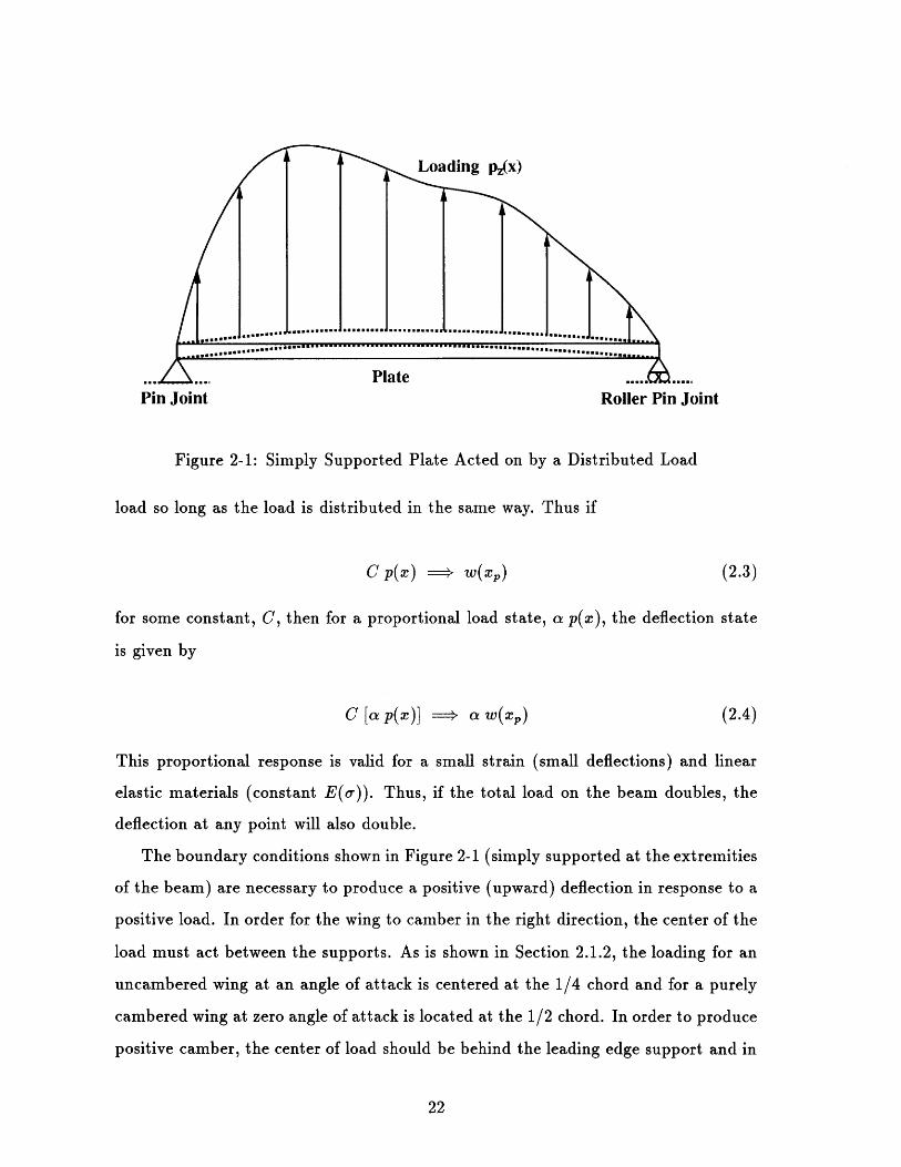
Figure 2-1.
The elastic deflection of a bending plate can be described by the Bernuolli-Euler
plate equation given in [9]:
D w(x = P(X) (2.1)
Where the plate stiffness, D, is given in terms of the elastic modulus, E, Poisson's
ratio, v and the thickness, h as
Eh 3
D 12(1 - (2.2)The deflection at some point 12(1 - 2)
The deflection at some point xp,w(xp), is proportional to the magnitude of the
Pin Joint Roller Pin Joint
Figure 2-1: Simply Supported Plate Acted on by a Distributed Load
load so long as the load is distributed in the same way. Thus if
C p(x) == w(z,) (2.3)
for some constant, C, then for a proportional load state, a p(x), the deflection state
is given by
C [a p(x)] == a w(xp) (2.4)
This proportional response is valid for a small strain (small deflections) and linear
elastic materials (constant E(o)). Thus, if the total load on the beam doubles, the
deflection at any point will also double.
The boundary conditions shown in Figure 2-1 (simply supported at the extremities
of the beam) are necessary to produce a positive (upward) deflection in response to a
positive load. In order for the wing to camber in the right direction, the center of the
load must act between the supports. As is shown in Section 2.1.2, the loading for an
uncambered wing at an angle of attack is centered at the 1/4 chord and for a purely
cambered wing at zero angle of attack is located at the 1/2 chord. In order to produce
positive camber, the center of load should be behind the leading edge support and in

front of the trailing edge support. This requires that the leading edge support must
be in front of the 1/4 chord point in order for the uncambered wing to camber under
the initial flat plate load. Further, the trailing edge support should be behind the
1/2 chord point to maintain positive camber for a purely cambered loading. The best
performance is obtained for boundary conditions as close to the leading and trailing
edges as possible.
2.1.2 Airfoil Theory
Much aerodynamic theory has been developed to describe the behavior of lifting
bodies. A wing of sufficiently high aspect ratio can be described in terms of cross
sectional airfoil shapes at its spanwise stations. The flow around such a wing has a
very small velocity component in the spanwise direction such that it can be modeled
as a two-dimensional flow around the various airfoil sections. Examining the behavior
of airfoils in a two-dimensional flow gives a good approximation of the actual flow over
the wing at various points along the span. Generally, the lift and drag performance
of airfoil sections can give a good indication of the lift and drag performance of the
entire wing.
The theory of thin airfoils, as given by Von Mises in [7], gives an approximate
solution for the flow around a thin airfoil, and thus the lift, in terms of the vorticity
distribution along the camberline, y(x). The vorticity distribution, -y(x), is deter-
mined from the camberline of the airfoil by enforcing the conditions that there is
no flow across the camberline (i.e. the flow is tangent to the camberline) and that
7y() goes to zero at the trailing edge (thus enforcing the Kutta condition). The flow
around the airfoil that is induced by such a I(z) distribution is a good approximation
to the flow around a thin airfoil with the same camberline.
The lift due to this vorticity distribution can be expressed in a non-dimensional
lift coefficient as
2 (/2C, = cV -/ 2 ( x) dx (2.5)
c Vo J-c/ 2

where c is the chord of the airfoil and V, is the freestream flow velocity. For a straight
camberline at an angle to the freestream flow of a, the lift coefficient is
C 1 = 27ra (2.6)
Similarly, the lift coefficient due to a curved camberline given in terms of the max
camber, e, at zero angle of attack to the flow (a = 0) is
Cl = rE (2.7)
Combining these two results for a general cambered airfoil at some angle of attack
gives
C1 = 27ra + -re. (2.8)
The moment due to the pressure distribution is given by
Sc/2M = - /2 p() (x- zm) dx. (2.9)
where xm is the point that the moment is acting around. In most cases, the moment is
calculated around the 1/4 chord since the moment is independent of the lift when it is
calculated around the 1/4 chord. For the uncambered airfoil, this integral evaluates to
zero implying that the center of lift of the flat plate is at the 1/4 chord. Performing
this same integral for the cambered airfoil at zero angle of attack shows that the
moment around this point is equivalent to the lift force acting at the 1/2 chord point.
Thus the center of lift for the pure camber case is located at the 1/2 chord.
The location of the center of lift for a general airfoil having some non-zero camber
magnitude and at some non-zero angle of attack depends on both the amount of
camber and the angle of attack. Because camber produces lift at the 1/2 chord while
angle of attack produces lift at the 1/4 chord, the amount of lift produced by each of
these factors determines where the center of lift is located, and the magnitude of the
lift at that point.

Traditional aerodynamic theory describes airfoils that have an arbitrary but fixed
amount of camber. The lift and drag forces are usually described in terms of nondi-
mensional coefficients that do not depend on the size of the airfoil or the strength of
the fluid flow. The lift coefficient of these fixed geometry airfoils is proportional to
their angle of attack. The relationship between angle of attack and lift coefficient is
described by the lift curve for that airfoil. Before stall, all inviscid airfoils have a lift
curve that is linear with a positive slope equal to 27r. An uncambered airfoil has a lift
coefficient equal to 0 at zero angle of attack. A cambered airfoil on the other hand has
a positive amount of lift at zero angle of attack. The lift curve of the cambered airfoil
is still 27r and is simply shifted upward from the uncambered lift curve. The more
camber an airfoil has, the more its lift curve is shifted upward from the uncambered
airfoil. The additional lift produced by camber is linearly proportional to the amount
of camber. The lift curves for various fixed geometry airfoils is shown in Figure 2-2
as well as in [8].
2.2 Elastic Airfoil Theory
The behavior of elastic airfoils can be described be combining simple plate theory
with simple airfoil theory resulting in an aeroelastic description of the flexible airfoil.
Airfoil theory describes the amount of lift that is generates by the airfoil and how
that lift is distributed. Beam theory describes how a beam bends under load. The
airfoil lift loads bend the beam and shape of the beam describes the camber of the
airfoil. The derivation of the linear aeroelastic theory is relatively straight forward,
but does require a few slight modifications to each of the theories. The deformation
response of the bending beam depends on the actual lift force of the airfoil rather
than the lift coefficient. Thus, when describing the behavior of the elastic airfoil in
terms of the traditional lift curve, it is also necessary to look at the lift of the airfoil
at each point on the curve.

2.2.1 Linear Theory of Flexible Airfoils
For a flexible airfoil, as the angle of attack increases, the camber increases and
thus the coefficient of lift will continually rise at a rate faster than the traditional lift
curve. For a given camber and coefficient of lift, the angle of attack can be found
from traditional cambered airfoil lift curves. However, the camber increases as the lift
coefficient increases. Thus the lift curve slope for a flexible airfoil should be greater
than the traditional lift curve slope of 27r. Figure 2-2 shows the lift curves of fixed
geometry airfoils with different amounts of camber and the lift curve for an automatic
camber adjusting airfoil. It shows how the lift curve slope is increased by the changes
in camber.
ClFlexible Airfoil
Fixed GeometryCamber > 0%
Slope = 2n
Camber = 0%Slope = 2n
Figure 2-2: Lift Curves for a Flexible Airfoil and Rigid Airfoils of Various Camber

2.2.2 Stiffness Parameter
The two major elements which determine the magnitude of a flexible airfoil's
camber are the stiffness of the airfoil and the strength of the aerodynamic loading.
The interaction and balancing of these two forces determines the amount of bend in
the plate, and thus the amount of camber in the airfoil.
In order to determine the exact bending behavior of the airfoil, the bending stiff-
ness and aerodynamic forces are equated in a coupled aerodynamics, bending plate
equation:
D x = Pz (s) (2.10)
where D is the plate stiffness, w(x) is the deflection of the plate at any point, x, and
p(x) is the aerodynamic pressure load applied to the plate at any point, x. From
this equation it is easy to see that increasing the load, p(x) causes the plate to bend,
increasing the camber, and that increasing the elastic plate modulus, D, causes the
plate to bend less, decreasing the camber.
For a given operating point with a fixed fluid dynamic pressure, q, and given an
airfoil section of chord length, c, and plate stiffness, D, the camber response of the
wing to the loading can be described by a nondimensional stiffness parameter, K.
K = D (2.11)
This stiffness parameter describes the relative strength of the restoring force of
a flexible plate and the aerodynamic forces of the flow. Larger values of K describe
stiffer airfoils with respect to the flow. Airfoils that have the same relative strengths
of the plate and the flow, will have the same cambering behavior for specific angles
of attack. Thus, the slope of the lift curve is related to the stiffness parameter, K.
The stiffer the airfoil, the less it cambers and thus the lower the lift curve slope. The
limiting case of this is when the airfoil becomes infinitely stiff. At this point the
airfoil does not camber at all and thus the lift curve matches that of a symmetrical,
rigid airfoil. Smaller values of K describe more flexible airfoils with respect to the

flow. As the stiffness, K, goes down, the airfoil cambers more and thus the slope
of the lift curve goes up. The limiting case of this is a an airfoil made with a very
flexible material such as a cloth sail. A sail cambers to its full extent with minimal
load and thus its lift curve in the cambering region jumps to full camber immediately
with no proportional response. In between these two limits is the K range for an
automatic camber adjusting airfoil. The Lift Curves for automatic camber-adjusting
airfoils with different K values are shown in Figure 2-3.
Figure 2-3: Lift Curves for Airfoils of Various K Values
2.2.3 Critical Stiffness
The stiffness that results in an infinite lift curve slope is defined as the critical
stiffness ,K,,it. At this value of the stiffness parameter, the camber of an airfoil at zero
angle of attack results in exactly the proper amount of lift to sustain that camber.
The airfoil can operate in equilibrium at any amount of camber without a change in
angle of attack. Thus the camber is undetermined for this stiffness at zero angle of
attack.

The critical stiffness depends, in part, on the distribution of the plate stiffness,
D. For a constant D, the value of Kcrit is calculated by Widnall et. al. in [10] to
be 1.4. For a case where the plate stiffness varies, this value can change. In the
case of a NACA 0012 airfoil made from a constant modulus, isotropic material, D
will be larger in the center, due to the greater thickness, than it is near the leading
and trailing edges where the airfoil is much thinner. If for this case an average plate
modulus Dave is used in calculating K, then the value of Kcit is higher than 1.4.
For values of K below the critical stiffness, any initial camber at a fixed angle of
attack results in a full divergent deflection of the camberline. Thus in a theoretical
aerodynamic sense, the airfoil undergoes static aeroelastic divergence at the critical
stiffness. From a structural point of view, however, it is still possible for the aero-
dynamic forces and the plate structure to achieve an equilibrium for values of the
stiffness parameter below Kcrit. A cambered airfoil at some positive lift but negative
angle of attack produces pressure forces that would cause a flexible airfoil to camber.
By fixing the lift of the wing and allowing the angle of attack of the wing to adjust
to changes in the camber, it is possible to achieve an elastic equilibrium for values of
K less than Kcit.
The theoretical lift curve in Figure 2-3 shows that for values of K below Krit,
the lift curve slope is negative. This occurs when the increase in loading causes the
airfoil to camber to such an extent that the increase in lift due to camber is greater
than the increase in the restoring force of the beam. Such negative lift curves would
be impossible to achieve in a wind tunnel or other experimental situation, but is
relatively easy to achieve numerically or for applications to craft where the lift is
determined rather than the angle of attack of the airfoil.
2.2.4 Effect of Spar Placement
The stiffness parameter defined in Equation 2.11 is based on the boundary con-
ditions at the leading and trailing edge points. However, this boundary condition
cannot be realized in a real wing because the spars that enforce the boundary con-
ditions cannot be located at the leading and trailing edges. Since the airfoil has no

thickness at the leading and trailing edges, a spar located there would also have no
thickness and thus no strength. In real wings, these spars must be placed where the
airfoil has significant thickness so that a structurally efficient spar can be used.
For such real wings, the spars are placed closer to the mid chord where the airfoil is
thicker. However, the spars cannot be placed arbitrarily as explained in Section 2.1.1.
For many applications the structural considerations of the spars are an important
design limitation and the designer is forced to maximize the spar thickness to support
the loads on the wing. Thus the spars are placed as close to the thickest part of the
airfoil as possible. It has been determined (mainly through working designs) that the
leading edge spar should not be much further back than the 10% chord point and the
trailing edge spar no further forward than the 70% chord point. The portion of the
airfoil in front of the leading edge axle and behind the trailing edge axle should be
made from a much stiffer material than the flexible region so that there is no bending
of the chordline in these regions.
Placing the spars at locations other than the leading and trailing edges has a large
effect on the value of the stiffness parameter of the airfoil. Placing the spars closer
together acts to effectively stiffen the airfoil in two ways. First, the flexible region
between the spars is smaller and making the plate seem stiffer. Secondly, some of the
load acts on the airfoil regions in front of and behind the spars. Thus, the load acting
on the flexible section is diminished and the load acting beyond the spars acts to
decamber the airfoil. This effect was quantified by Widnall et. al. in [10] for the spar
location effect on the critical stiffness. By applying a curve fit to numerical results,
K,it for an airfoil with constant plate stiffness between the spars is given by
Kcrit = 1.3 - 2.6 XL.E. Spar 2.3(1 - T.E. Spar ) (2.12)c c
where zL.E. Spar and XT.E. Spar are the x locations of the leading and trailing edge
spars.
2.3 Two-Dimensional XFOIL Tests
The viscous drag of an airfoil is determined by many characteristics of the airfoil
shape and operating point. The drag polar for an airfoil shows the relationship of
drag to lift coefficient for the airfoil. Changes in the camber of an airfoil change the
lift coefficient associated with the minimum drag coefficient for an airfoil. In general,
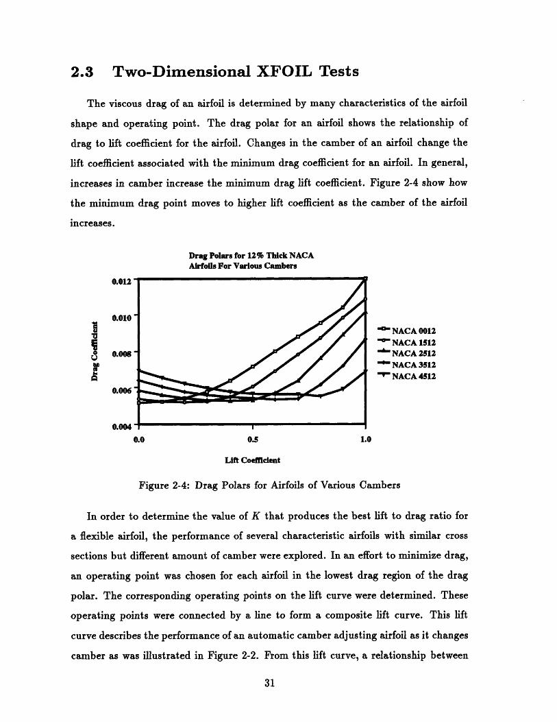
increases in camber increase the minimum drag lift coefficient. Figure 2-4 show how
the minimum drag point moves to higher lift coefficient as the camber of the airfoil
increases.
Drag Polars for 12% Thick NACAAirfoils For Various Cambers
0.012
0.010NACA 0012
- NACA 15120.008 " NACA 2512
V NACA 3512' NACA 4512
0.006
0.0040.0 0.5 1.0
Lift Coefficient
Figure 2-4: Drag Polars for Airfoils of Various Cambers
In order to determine the value of K that produces the best lift to drag ratio for
a flexible airfoil, the performance of several characteristic airfoils with similar cross
sections but different amount of camber were explored. In an effort to minimize drag,
an operating point was chosen for each airfoil in the lowest drag region of the drag
polar. The corresponding operating points on the lift curve were determined. These
operating points were connected by a line to form a composite lift curve. This lift
curve describes the performance of an automatic camber adjusting airfoil as it changes
camber as was illustrated in Figure 2-2. From this lift curve, a relationship between

C and camber was determined.
The program, XFOIL (See [3] for program details) was used to generate the lift
and drag data for airfoils of various camber and lift coefficient. The NACA x515
section was chosen for the thickness and camber distribution. The Stiffness of a
particular airfoil was related to a proportionality between camber and lift coefficient
as
Flexibility camber (2.13)camber
For example if the flexibility, was chosen to be 10, then at a C, of 0.1, the NACA
1515 (1% camber) was chosen; for a C1 of 0.2, a NACA 2512 (2% camber) was chosen;
for a C, of 0.3, a NACA 3512 (3% camber) was chosen; etc. In this way, a lift curve
was constructed from the various operating points of the airfoil as represented by the
various fixed geometry airfoils. Lift curves were constructed for various flexibilities.
The results showed that the optimal lift to drag performance was attained when the
camber to C1 ratio was near 5. For this flexibility, a C1 change of 0.1 results in a
2% camber change. For this flexibility, the amount of lift produced by the camber
of the airfoil is about 3 times the amount of lift produced by angle of attack. Put
another way, for high reynolds number airfoils, the optimal lift to drag ratio occurs
when about 3/4 of the lift is produced by camber and the remaining 1/4 by angle of
attack.
The lift curves generated by these XFOIL tests show the relationship of lift curve
slope to stiffness for a two-dimensional airfoil. A few of the lift curves are show in
Figure 2-5. The slope of the lift curve clearly varies with the stiffness of the airfoil.
As the flexibility of the airfoil goes up (stiffness goes down), the slope of the airfoil's
lift curve increases. For a high enough flexibility, the slope becomes negative.
The results of these XFOIL tests also give a good indication of the reduction in
viscous drag of flexible wings over rigid symmetric wings. The drag polars for various
flexible airfoils are shown in Figure 2-6. The drag on the rigid airfoil (flexibility =
0) increases rapidly as the lift coefficient increases because the angle of attack is also
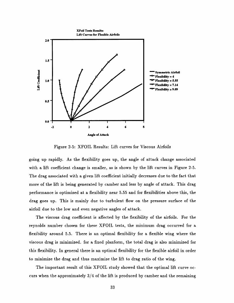
XFoll Tests Results:Lift Curves for Flexible Airfoils
2.0
1.5
Symmetric AirfoilT *- Flexibility = 4
1.0 "- Flexibility = 5.55- Flexibility = 7.14
Flexibility = 9.09
0.5
0.0
-2 0 2 4 6 8
Angle of Attack
Figure 2-5: XFOIL Results: Lift curves for Viscous Airfoils
going up rapidly. As the flexibility goes up, the angle of attack change associated
with a lift coefficient change is smaller, as is shown by the lift curves in Figure 2-5.
The drag associated with a given lift coefficient initially decreases due to the fact that
more of the lift is being generated by camber and less by angle of attack. This drag
performance is optimized at a flexibility near 5.55 and for flexibilities above this, the
drag goes up. This is mainly due to turbulent flow on the pressure surface of the
airfoil due to the low and even negative angles of attack.
The viscous drag coefficient is affected by the flexibility of the airfoils. For the
reynolds number chosen for these XFOIL tests, the minimum drag occurred for a
flexibility around 5.5. There is an optimal flexibility for a flexible wing where the
viscous drag is minimized. for a fixed planform, the total drag is also minimized for
this flexibility. In general there is an optimal flexibility for the flexible airfoil in order
to minimize the drag and thus maximize the lift to drag ratio of the wing.
The important result of this XFOIL study showed that the optimal lift curve oc-
curs when the approximately 3/4 of the lift is produced by camber and the remaining

- Symmetric AirfoilO Flexibility = 4= Flexiblity = 5.55
Flexibility = 7.14Flexibility = 9.09
0.5 1.0 1.5 2.0
Lift Coefficient
Figure 2-6: XFOIL Results: Drag Polars for Viscous Airfoils
angle of attack. The slope of this optimal lift
than the rigid airfoil lift curve slope.
curve is approximately 3 times
2.4 Three-Dimensional Extension
Airfoil theory gives a great deal of information about the flow over the wing in
terms of lift, but cannot account for the span affects on the flow and the resulting
induced drag. The flow over finite span wings differ from the flow over airfoils because
the lift is zero at the wing tips and varies along the span of the wing. The spanwise
variation in lift results in a sheet of vortices trailing downstream from the wing. This
shed vorticity results in a downward fluid velocity often referred to as downwash. The
downwash velocity adds to the freestream velocity causing a change the apparent angle
of attack often referred to as the induced angle of attack, ai. This induced angle of
attack changes the amount of lift that the wing generates as well causing induced
drag.
XFoll Test Results:Drag Polars for Flexible Airfoils
0.012
0.010
0.008
0.006
0.004
1/4 by
greater

The performance of finite wings is affected by the induced downwash. The induced
angle of attack reduces the angle of attack of the wing thereby reducing the lift.
However, since the actual angle of attack, ca, of the wing is referenced to the far
field flow (which remains unchanged), the wing appears to have lower lift than airfoil
theory predicts and the slope of the lift curve for the wing is reduced. This effect is
shown in Figure 2-7.
2-D lift at xa
Finite Span Lift at aa /
2-D lift curveSlope = 2
/ lift curve forfinite span wing
Figure 2-7: Lift curve for a Finite Wing
The magnitude of ac depends on the strength of the downwash with respect to
the free stream strength. The downwash depends on the gradient of the spanwise
loading of the wing. Higher aspect ratio wings have lower spanwise loading gradients
and thus smaller downwash and resulting in a smaller induced angle of attack for a
given lift coefficient. The higher the aspect ratio of the wing, the smaller the induced
angle of attack will be in relation to the geometric angle of attack, and thus the closer
its lift curve slope will be to the theoretical two-dimensional slope of 2r.
The minimum induced drag occurs when the downwash is a constant value across
the wing. This occurs when the spanwise lift distribution is elliptical as shown in

Figure 2-8. Rigid wings have been designed with some combination of spanwise chord
distribution, twist distribution or camber distribution. An elliptic chord distribution
with no twist or camber produces an elliptic lift distribution for all angles of attack.
However, this uncambered wing will, in general, not be as efficient as a properly
designed camber wing for the same application. However, a fixed camber distribution
that produces an elliptic lift distribution for one angle of attack will, in general, not
produce an elliptic lift distribution for other angles of attack.
Lift DistributionL(y)
Figure 2-8: Elliptic Lift Distribution for a Finite Wing
For such an elliptically loaded wing, the lift curve slope is given by
m = (2.14)1 + "__Oa.wAR
where m is the lift curve slope for the finite span wing, mo is the 2xr theoretical
two-dimensional lift curve slope and AR is the aspect ratio of the wing.
Tapered planforms can very nearly match the elliptic span loading. According
to Glauert [4], a tip chord to root chord ratio between 0.3 to 0.5 produces the best

approximation of an elliptic span loading. The lift curve slope for a finite span tapered
planform is shown compared to that of an elliptic planform over a range of aspect
ratios in Figure 2-9.
Comparison of Elliptic and Tapered Planforms
• Tapered Planform" Elliptic Planform
.... 2-D slope
0 10 20 30 40
Aspect Ratio
Figure 2-9: Lift Curve Slopes of Tapered and Elliptic Planforms
2.4.1 Flexible Wings of Finite Span
The performance of finite span flexible wings are affected in much the same way
as rigid wings. Downwash affects the lift curve of the flexible wing in the same way
as it affects rigid wings. The lift curve slope is reduced and induced drag is formed.
However flexible wings have a theoretical two-dimensional lift curve slope greater than
27r, so it is possible for a finite span wing to have a lift curve slope greater than 27r
as well.
However the effective strength of the flow changes as well when the aspect ratio
changes. This changes the critical stiffness value, Keit. For high aspect ratio flexible
wings, this effect is summarized in Equation 2.15 from as defined by Widnall et. al.

in [10].
Kwing = Kairfoa (1 - 1.3(2.15)
Thus, Ket i,g is decreased for a finite span wing.
This theory was developed assuming that each spanwise cross-section of the plate
behaved like an ideal two-dimensional plate and assumed the proper chordwise bend-
ing for the local loading only. However, in a real wing, the plate is continuous and
thus the bending at any point along the plate will be affected by the loading over
the entire plate (See Mansfield [6]). For high aspect ratio wings, the gradient of the
loading in the spanwise direction are much less steep and the spanwise stations are
able to more closely conform to the predicted beam behavior. Lower aspect ratios on
the other hand, have very steep gradients in the load and thus the camber response
conforms less closely to the local loading.
2.4.2 Effective Stiffness
The question of the determining the stiffness parameter for a finite span wing has
been addressed by Widnall et. al. in [10]. The stiffness of the wing is determined
by an effective stiffness test and non-dimensionalized in the same way as the two-
dimensional stiffness parameter. This method involves applying a load to the wing
and measuring the deflection of the wing. Specifically, the test involves applying
a uniform distributed span load, P(load/unit length), to a line that lies halfway
between the axis of rotation of the two spars as Shown in Figure 2-10. The effective
stiffness of the wing, S 1ff, is then given in terms of the deflection at the midspan,
Wmidspan as
PSe -= (2.16)
Wmidspan
The effective stiffness gives a single stiffness value for a wing that may or may not have
a constant value for K over the span. The choice of measuring the deflection at the
midspan rather than the root or tip is relatively arbitrary. However, this convention

is used by Widnall et.al. in [10], and is presented here to keep notation consistent.
Span Load, P
Figure 2-10: Effective Stiffness Test Setup
The critical dynamic pressure of the wing, qit can be determined from the effec-
tive stiffness by
1qcrit = ASef(1 1.3
AR
(2.17)
where A is a coefficient around 0.1.
Since Real wings are constructed from a particular material with a particular elas-
tic modulus, thickness distribution and spar placement, once it has been constructed,
it is virtually impossible to modify the structural properties and in particular the
plate stiffness. For such a real wing, the stiffness changes as the dynamic pressure
changes rather than the plate stiffness. Thus, the critical stiffness, Koit is related to
a critical dynamic pressure, qrit. The critical stiffness for the wing, K it wing is given
as
DKerit wing - D 3
qrit (S)3 (2.18)

In general, the exact value of K,,it for a given wing planform should be determined
numerically or experimentally, but the effective stiffness test provides a good estimate
for the cases where numerical or experimental analysis is unavailable.

Chapter 3
Numerical Methodology
The study of the behavior fo flexible wings is accomplished by modifying and com-
bining two existing computer programs to solve for the steady aeroelastic behavior of
the flexible wings. The Fluid Dynamics are modeled with a vortex lattice program
originally coded by Harold Youngren and the Structure is modeled in the ADINA
finite element program. The vortex lattice program solves for the aerodynamic loads
due to an inviscid flow over the wing. These loads are then passed to the finite
element program, ADINA, that models the structural behavior of the wing. The
ADINA program solves for the linear elastic static response of the wing structure
to the steady aerodynamic loads. The static deflection state is then passed back to
the vortex lattice program which solves for a new set of loads given the new wing
geometry. The new loads are passed to the finite element program and it solves for a
new deflection state. This process continues until the solution converges to a steady
equilibrium state.
3.1 Vortex Lattice Aerodynamic Model
The potential flow over a thin wing can be modeled by a distribution of vorticity
on the surface of the wing and the corresponding vorticity shed into the wake (See
[8]). The vortex lattice program discritizes the vorticity into a finite number of bound
"horseshoe" vortices which have a vortex segment bound to the surface of the body

and two trailing segments that extend downstream with the wake. The circulation
of each segment of the horseshoe vortex is the same such that the correct amount of
vorticity is shed into the wake from the vortex according to Helmholtz's law. The total
circulation of the wing is then modeled by a group of these horseshoe vortices that
are distributed over the surface in both the chordwise and spanwise directions. The
vorticity on the wing at any point is then modeled by varying strengths of the bound
segments of the horseshoe vortices near that point. From the vortex distribution and
strengths, the lift and drag of the wing can be modeled in a discrete set of loads.
3.1.1 Geometry
The wing is represented in a 3-D cartesian space with the x axis pointed down-
stream along the root chordline, the y axis pointed in the right spanwise direction
and the z-axis pointed up. The origin is located at the leading edge of the root of the
wing. The freestream vector is assumed to be at a small angle to the x-axis allowing
the use of small angle linearizations. The leading edge of the wing can be swept (an
angle to the y-axis) and the wing can have dihedral out of the x - y plane.
The full wing planform is symmetric across the x - z plane. The full load state
can be determined from the load state on only one half of the planform (in this case
the +y half). The load on the other half of the planform is the mirror image of that
load state. Thus by treating the x - z plane as a symmetry plane, only half of the
wing needs to be constructed. This half, referred to as the real wing, is constructed
by specifying the geometric placement of the vortices and the collocation points.
The other half of the planform, referred to as the image wing, is constructed by the
enforcement of a reflective boundary condition on the x - z plane.
The wing is sectioned into spanwise strips. Each of these strips is represented by
the chordline at each edge. The edges of these strips are parallel to the x - z plane
but may be at a different angle of attack than the root chordline. The camberline
is prescribed by a set of (x, y, z) coordinates at the edge of each strip. Thus, all
geometric considerations such as sweep, twist, and dihedral can be accounted for.
The spanwise geometry is assumed to be linear between the strips.
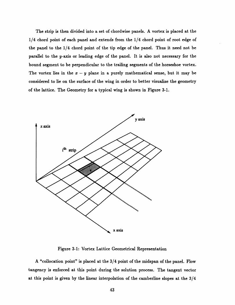
The strip is then divided into a set of chordwise panels. A vortex is placed at the
1/4 chord point of each panel and extends from the 1/4 chord point of root edge of
the panel to the 1/4 chord point of the tip edge of the panel. Thus it need not be
parallel to the y-axis or leading edge of the panel. It is also not necessary for the
bound segment to be perpendicular to the trailing segments of the horseshoe vortex.
The vortex lies in the x - y plane in a purely mathematical sense, but it may be
considered to lie on the surface of the wing in order to better visualize the geometry
of the lattice. The Geometry for a typical wing is shown in Figure 3-1.
axis
z axis
ilh strip
x axis
Figure 3-1: Vortex Lattice Geometrical Representation
A "collocation point" is placed at the 3/4 point of the midspan of the panel. Flow
tangency is enforced at this point during the solution process. The tangent vector
at this point is given by the linear interpolation of the camberline slopes at the 3/4
chord point of the two edges of the panel. Since the camberline data set is made
of discrete (x, y, z) points, the slopes are interpolated from the data set by the use
of cubic splining. Again, this point lies on the x - y plane for purely mathematical
purposes, but may be considered to lie on the surface of the wing for visualization
purposes.
In order to accurately represent the flow, the corners of the panels in one strip
match with the corners of the panels in the next strip. Thus there are the same
number of vortices in each strip and the coordinate of the tip end point of the bound
segment of a vortex in one panel matches the root coordinate of the bound segment
of a vortex in the next panel. Thus there are a set of continuous vortex segments
extending form the root to the tip that vary in strength in the spanwise direction and
shed the differential vorticity downstream.
3.1.2 Formulation of the Vortex Lattice
Once the geometry of the lattice has been established, each of the horseshoe
vortices can be described by the location of the two endpoints of the bound segment
of that vortex, r, and r'. The velocity vector Ui at any point in the flow due to the
circulation around the vortex can be calculated using the Biot-Savart Law
= r (3.1)47r P - ,
and integrating along the three segments of the horseshoe vortex. By assuming a unit
circulation strength, we can determine the influence of that horseshoe vortex on each
of the control points. It is also easy to calculate the influence of an image vortex on
the control points by setting the y coordinate of the endpoints to be the negative of
the actual vortex. By calculating the influences for each of the vortices, an "influence
coefficient matrix" can be constructed.
3.1.3 Determination of vortex strength
The actual strengths of each of the vortices should cause the flow to be tangent
to the surface at each of the collocation points. The normal vector to the surface at
each of the collocation points can be determined from the geometry. By setting the
vector dot product of the normal vector with the velocity vector that is induced by
the vortices to be zero, the flow is enforced to be tangent to the surface. Since the
induced velocity is caused by all the vortices, the flow tangency at any control point
can be expressed by a linear equation involving all N vortices. The N equations for
the N control points, form a N x N system of linear equations that can be solved
simultaneously for the N vortex strengths. In the program, the solution to this matrix
equation is found using Gaussian Elimination since the Matrix is, in general, fully
populated.
3.1.4 Solution and Discrete Forces
The strength of a given vortex is related to the lift force it generates by the
Kutta-Joukowsky Theorem. Given the bound segment of the horseshoe vortex, ', is
the vector sum of the position vectors of the endpoints, r', and r2, as
c = r2 - rl. (3.2)
The force vector that the mth vortex generates is then given by
Fm = m Um x cm (3.3)
where u'4 is the total velocity vector and Fm is the vortex strength of the mth vortex.
These discrete forces are stored so that they can be sent to the finite element pro-
gram. The finite element program, takes as an input, the modulus of the material.
This modulus is expressed in a dimensional way, so in order to describe the relation-
ship of the loads to the stiffness of the wing in terms of the stiffness parameter, K,
the loads need to be dimensionalized. The dynamic pressure and lift coefficient are

chosen so that the total lift is 100.
3.1.5 Total Forces and Non-Dimensional Force Coefficients
Summing the discrete force vectors gives the total force on the wing. The total
force of the full wing takes into account the image half of the wing as well as the real
half.
N
Ftotal = 2 E Fm (3.4)m=1
This total force can be resolved into drag and lift forces by taking the dot products
of the Total force vector with the freestream and its normal respectively.
L = Ftotai * [-(sin a)i + (cos a)k] (3.5)
D = Ftota . [(cos a)i + (sin a)lk] (3.6)
The lift and drag forces can be expressed more generally by non-dimensional force
coefficients. The lift coefficient is defined as
CL = 1 (3.7),PV' Sref
where L is the total lift, ipV, is the free stream dynamic pressure and S,,f is the
surface area of the wing. Similarly, the drag coefficient is defined as
CD 1 (3.8)C PV2Sref
where D is the total drag.
3.1.6 Trefftz Plane Drag Calculation
The drag calculated by Equation 3.6 is very sensitive to numerical errors. In most
cases, the force vectors near the leading edge of the wing have substantial forward

components and the vectors near the trailing edge of the wing have substantial aft
components. These should mostly cancel out leaving only the induced drag compo-
nent of the total force. A small error in these vectors, however, could result in a large
error in the drag vector given all of the vector cancellation. Thus the drag calculation
has a very low accuracy.
One solution to this problem is to calculate the induced drag by looking at the
induced velocities in the wake far downstream from the wing. This is most commonly
done by constructing a plane, known as the Trefftz Plane, parallel to the y - z plane
in the far field wake as shown in Figure 3-2, and looking at the induced flow velocity
in that plane.
wake vortex sheet
Trefftz Plane
Figure 3-2: Trefftz Plane Intersecting Wake Vortex Sheet
The work done by the induced drag force can be calculated from the residual
velocity vector, W. The induced velocity field W is irrotational and can be expressed
as the gradient of a crossflow potential.
W = V0 (3.9)
The kinetic energy per unit volume can be written as simply pj jll 2. Thus the
induced drag is simply the integral of the kinetic energy per unit volume over the

entire Trefftz Plane.
D = Wp J II|I 2 dy dz (3.10)
D = ~p V -. V dy dz (3.11)
By taking a contour that completely encloses the wake, the area integral becomes, by
Gauss's Theorem, a contour integral.
D = - wp w - ds (3.12)
The velocity component of w' normal to the wake is the same on either side of the
wake cut. Thus the contour integral can be changed into a line integral in terms of
the potential jump across the wake.
D = -p Aq- dl (3.13)
The potential jump, AO, at any spanwise station of the wake must be equal to the
bound circulation, r, at the point on the wing directly upstream of that point. Thus
it is trivial to calculate the Trefftz Plane drag by taking the integral along the wing
of the bound circulation, P(y).
D = -lp r(y) - -n dl (3.14)
Given the discrete nature of the circulation distribution on the wing, r, at any
spanwise station can be expressed as a sum of the horseshoe vortex strengths at that
spanwise point. Thus the integral can be evaluated by summing over all of the N
bound vortices on the wing.
D = -p r. w - An (3.15)
This total drag can be expressed in terms of the drag coefficient as in Equation 3.8.

Both the trefftz plane analysis and the vector analysis are calculated by the vortex
lattice program. Both are given as output for comparison, however it is generally
accepted that the trefftz plane analysis gives the better result and this result will be
given as the total drag coefficient for the wing in the results.
3.1.7 Vortex Lattice Program Overview
The actual program that is used in this study is a modified version of a vortex
lattice program written by Harold Youngren for the Project Athena Todor facility
in 1990. The geometric shape of the wing is read into the vortex lattice program
from a datafile. The user then inputs the desired lift coefficient and the stiffness of
the wing. The program determines the influence coefficint matrix and solves for the
vortex strengths at the desired lift coefficient and determines the angle of attack of
the reference line at the root of the wing. The program also determines the downwash
distribution along the span of the wing and the induced drag of the wing.
The accuracy of the method depends to a large degree on the geometry of the
wing and the number and placement of the vorticies. Some of the problem that arise
in the accuracy are due to sweep discontinuities at the root and the drastic variation
in spanwise loading at the tip (See Moran [8)). Given the low sweep of the wings in
this study as well as the large number of vorticies placed on the wing, the method
should be quite accurate. In particular, the accuracy of the lift is much better than
the accuracy of the drag and by calculating the drag in the Trefftz Plane, much of
this inaccuracy is overcome. for the very linearized models in this study, the accuracy
of the method is more than adequate.
3.2 Finite Element Model
The elastic response of a structure to an applied load state can be analyzed nu-
merically by breaking the structure into small pieces known as finite elements (See
[2]). Each of these finite elements is essentially a small plate acted on by a very
simple set of loads applied at discrete points within the element called nodes. Since

the elements are simple, it is easy to find their response to the simple load states that
can be applied to them. Then the entire structure can be put back together and the
more complex real load state applied to it. Each element feels some simple part of
that real load and responds accordingly. The response of the entire structure is then
the combination of the responses of all the elements put together.
By using the Principle of Virtual Work, the general response of each of the el-
ements to imaginary loads can be determined. The response is represented in an
influence matrix called the element stiffness matrix. This matrix describes the dis-
placements of each of the nodes of the element to imaginary loads applied to each of
the nodes.
By then assembling the elements into a mesh, the response of the entire structure
to an imaginary load state is determined. The element stiffness matrices are added
together into a much larger global stiffness matrix. This matrix describes the response
of each of the nodes in the entire structure to imaginary loads applied at any of the
other nodes. The response of the structure to the real load state is then simply a
combination of several imaginary load states.
3.2.1 Formulation of the Finite Element Mesh
The elemental boundaries are determined mainly by geometric constraints. A set
of points, called nodes, are defined on the midplane of the plate. These nodes define
the corners of the elements. The elemental boundaries are defined by lines connecting
the nodes. There are nodal degrees of freedom (d.o.f.s) defined at each node. Theses
d.o.f.s define the displacement and rotation of the structure at the nodes.
For the plate bending/stretching case that is modeled here, each node must have 5
d.o.f.s., the 3 displacements (u, v, w) and two rotations (0, and 0,). The displacements
u, v and w are in the x, y and z directions respectively, and 0, and 0, are the rotations
from the x axis and the y axis respectively as shown in Figure 3-3.

W
% OX
2
Node 1 C,
2
Figure 3-3: Nodal d.o.f.s Figure 3-4: Triangular Area Coor-dinates
3.2.2 Local Element Coordinate System
For the plate structure of the wing, a Finite Element mesh involving 3 node tri-
angular plate elements is utilized. These triangular elements utilize a generalized
triangular area coordinate system (1,C2, C3) as shown in Figure 3-4. Properties of
the element such as the displacement, strain or stress are only known at the nodes.
The properties of the element can be interpolated within the element by the use of
interpolation functions. The three node isoparametric triangular element has inter-
polation functions N1 , N2 and N3 .
N 1 = C1, N2 = 2, N3 = 3 = 1 - 1-2 (3.16)
The coordinates within the element are interpolated from the interpolation func-
tions with respect to the coordinates of the 3 nodes, (x, yl), (X2,y 2) and (xs,y 3).
X = NIxI + N 2 X 2 + N 3 X3 (3.17)
y = NXyl + N2 y2 + N3Y3 (3.18)
The Jacobian matrix to transform from the (Cl, C2, (3) coordinate system to the (x, y)
coordinate system is given by

J _= aoC aC (3.19)
0a2 a02
For the triangular elements, the determinant of the Jacobian is simply twice the are
of the triangle. The shape interpolation functions and the Jacobian matrix describe
the relationship between the local coordinate frame of the element and the global
coordinate frame of the entire structure.
3.2.3 Element Stiffness Matrix
Each of the elements is described by a element stiffness matrix. For triangular 3
node triangles, the element stiffness matrix describes the response of the structure to
imaginary unit loads or virtual loads at each of the nodes of the element.
The formulation of the element stiffness matrix comes from the principle of mini-
mum potential energy. The potential energy HpII, is defined as
S= U - W (3.20)
where U is the internal strain energy of the structure and W is the work done by the
applied loads. U and W are defined as
U = J { e}T [E]{e} dV (3.21)
W = J (X, y) w dA (3.22)
where {e} is the strain vector, [E] is the elasticity matrix, p, is the loading and w is
the deflection.
The variational form of the potential energy equation is given as
SII, = SU - SW (3.23)
The structure will tend toward a minimum potential energy state. This minimum
energy state can be found by taking SII, = 0. The element stiffness matrix [k] is

derived from the internal strain energy term, 6U.
The plate that models the flexible ceneterline of the wing, undergoes stretching
as well as bending due to the loads that are applied to it. The structural problem of
plate bending and plate stretching are, for an isotropic material, separable. The plate
bending case uses the plate bending modulus matrix, [D], to relate the out of plane
displacements w, 8, and 8, to the transverse loading p,. The plate stretching case uses
the plate stretching modulus matrix, [E], to relate the in-plane displacements u and
v to the in-plane loading p, and py. As long as the deflection state is small relative
to the plate dimensions, these problems remain separate and the FEM formulation
for each can be done separately.
For the bending plate case, the internal energy, U, for the element is formulated
as
1U = [J] IJJ dC2 dC1 (3.24)
The curvature matrix, [.], is defined as
O 2
-= 2 =[M] (3.25)By
2
-2 b2w
[M] is defined from geometry as
-(Y3 - Y)2
-(Y2 -- Y1)2 2(Y2 - Y1)(Y3 - Yl)
M -(e3 - i)2 -(- 2 - ")2 2(-2 -- 1 )(- 3 - ) (3.26)
2(-3 - -1)(Y3 - Y1) 2(-2 - 1)(Y2 - Y1) -2[(+3 - 1l)(Y2 - 1)(-2 - 1)(Y3 -- O1) 1
Then the energy, U, can be written
1 1 - (U = -f [M]T [D][M] dC d( 2 ]i (3.27)
giving U = if[k]bi, where [k]b is the bending stiffness matrix

kb = i [M]T [D][M] dG( d( 2] (3.28)
The bending stiffness matrix, [k]b, is a 9x9 matrix relating the three out-of-plane
deflections, w, 0, and 09, for the three nodes to the out-of-plane load, p,, and the
applied moments, M, and My, at the three nodes.
For the stretching plate case, the internal energy, U, for the element is formulated
as
U = [E[E] |J|1 dC2 dC1 (3.29)
Formulating the internal energy equation into the form U = q4r[k],' gives
k,= [B]T [E][B] t 11J11 dC2 d 1 (3.30)
where t is the thickness of the element, |JI is the determinant of the Jacobian Matrix
and [B] is the spatial derivative matrix
ON, 0 ON2 0 ON 3 0
1 0 0 0 aOc a a oC
[]-1 0 N 0 2 0 N 0B= 0 0 0 1 0aC2 aC2 a (3.31)
0 [J]-' 0 ON1 0 9N2 0 ON30 1 1 0 0~C at aCi
0 N1 0 ON2 0 ON3aC2 0a2 C(2
The stretching stiffness matrix, [k],, is a 6x6 matrix relating the two in-plane
deflections, u and v, for the three nodes to the in-plane loads, p. and py at the three
nodes.
The plate element must solve for both the bending and stretching of the structure.
Thus the element stiffness matrix needs to have both the bending and stretching terms
in it. By defining the element d.o.f. vector, ', to be
qe = LUi, v, U2, v 2, u s , v 3 , Wi, 9 x,1, O,1, W 2 , 9 x,2 ,9 y,2 , w 3 , Ox,3, Oy,3J (3.32)

then the element stiffness matrix, [k],, can be formed by combining the bending and
stretching element stiffness matrices [k]b and [k], to form a 15 x 15 matrix.
ke, = 0 (3.33)0 kb
3.2.4 Global Stiffness Matrix
The element stiffness matrix for each element relates the nodal responses of that
element to the applied nodal loads. By combining all of the element matrices together
such that the global d.o.f.s match, the global stiffness matrix can be constructed. This
global stiffness matrix relates the global displacements to the global loading state.
A given non-boundary node (one that is shared by more than one element), there
are terms in the element stiffness matrices of all the elements that share that node
which relate the displacement of that node to the forces applied at that node. The
terms in the global stiffness matrix for that node are then simply the sum of the
elemental terms. Each term of the global stiffness matrix is constructed by summing
all the terms that relate a given force to a given displacement of a given node.
3.2.5 Solution Method
Once the Global stiffness matrix is constructed, the solution involves simply find-
ing the solution of the system of algebraic equations that are given by the matrix.
The work term, 6W, gives the discritized load vector, Q. Thus from the global
stiffness matrix, [K], the d.o.f. vector, q, and the load vector, Q, we get the matrix
equation
[K]q= Q (3.34)
This matrix is solved by a general matrix solution technique. The solution is given
in terms of the d.o.f. vector, [q]. The displacements u, v and w for each of the nodes
are given in the solution vector, [q]. These displacements are printed out to a data
file so that they can be read by the input routine of the vortex lattice program.
3.2.6 ADINA program overview
The finite element program used for this study is the ADINA program developed
by ADINA R&D Inc.. The ADINA (Automatic Dynamic Incremental Non-Linear
Analysis) package is capable of performing finite element calculations for a wide va-
riety of problems, however, a very limited set of the capabilities of the package are
needed for this study. The program itself is licensed to the MIT Supercomputing
Facility and has been compiled to be run on the CRAY X-MP. For this study, ac-
cess to the CRAY X-MP has been through the experimental Transparent Computing
Module that has been developed by the MITSF.
The ADINA package consists of three programs, ADINA-IN, ADINA and ADINA-
PLOT. ADINA-IN is used to setup the Finite Element mesh from inputed geometric
and load information. ADINA-IN creates a formatted database containing all the
information so that a solution to the problem can be determined by ADINA. ADINA-
PLOT takes that solution and presents it in graphical or tabular formats that give
information about the problem that is requested by the user.
ADINA-IN exectues a series of commands contained in a ".in" file. This file
contains all the geometric information about the problem as well as the boundary
conditions loading and material type. It also contains information on how the mesh
should be created and what type of elements should be used. This study is interested
in the linear elastic behavior of flexible wings only. Thus, all materials have been
specified as ELASTIC in the ADINA input files such that the model will respond
in a completely linear way to the loading. The wing has been modeled with 3-node,
triangular PLATE elements. The formulation of these elements is done automatically
by the ADINA-IN program.
ADINA is the actual finite element solver. It takes the geometric information
from the ADINA-IN database and constructs the element stiffness matricies for all of
the elements. It then assembles the global stiffness matrix from the element stiffness
matricies. By inverting this matrix and the corresponding load vector, ADINA solves
for the deflections of all the nodal d.o.f.s for the structure.
This solution is formatted into a useful, readable output by the ADINA-PLOT

program. This program reads commands form a ".plot" file that contains information
about what aspects of the solution the user would like to study. In many cases, numer-
ical information about the structure such as the deflection or stresses are desired and
the ADINA-PLOT program can write a ".plist" file that contains such information.
3.3 Interaction of Numerical Programs
For the problem of the flexible wing solved by these numerical schemes, there is
an interaction of the aerodynamic forces and the structure. This interaction must be
modeled by the numerics. This interaction is handled by the programs in an iterative
fashion rather than solving the two systems simultaneously. The programs pass back
and forth information on the loads and the shape.
3.3.1 Geometric Relationship
To ease the interaction of the two numerical schemes, the mesh nodes of the finite
element portion of the program are chosen so as to match the load points of the vortex
lattice program. This allows trivial interaction of the two schemes. A node of the
finite element mesh is placed at center of the bound segment of each of the horseshoe
vortices. Thus, the lift force produced by that vortex acts directly at the node.
Many other nodes are placed so as to fill out the mesh. The placement of these
nodes is such that they lie on the spanwise edges of the vortex lattice strips. Thus,
the new camber distribution of the wing at each of these spanwise stations can be
easily splined directly from the nodal displacements at that station.
The vortex lattice itself is geometrically constructed so that the finite element
mesh that is constructed from it is well formulated. There are panel edges that
correspond directly to the locations of the axle boundary conditions. The panels are
placed such that the mesh has a good resolution in the flexible bending section of the
wing.

3.3.2 VL: Lift Load Information
The vortex lattice program generates a set of discrete aerodynamic loads that act
on the lifting wing. These loads act at the center of the bound vortex segment of
each of the horseshoe vortices. These load forces can be passed directly to the Finite
Element Program.
The vortex lattice is initialized with the the planform information and initial
camber information. For most of the data runs, the initial camber state is assumed
to be that of an uncambered wing. Thus the performance information can be assumed
to be related for both positive and negative loading cases.
Subsequent iteration steps read geometric information from the finite element
program. The finite element routine passes displacement information to the vortex
lattice program that it then turns into planform and camber information.
The vortex lattice program is set up to maintain a constant lift coefficient through-
out a data run. Thus the angle of attack will change at each iteration step as the
camber changes. This is necessary to prevent divergent behavior in the wing. It also
models the response of a real wing more accurately since real wings have a finite load
to lift and must respond to that lift requirement. It should be noted that this is
different from the behavior of such wings in wind tunnel experiments since in wind
tunnels, the angle of attack is usually fixed and the lift measured.
The vortex lattice program is a modified version of a progam that was originally
coded by Harold Youngren for use in the MIT Project Athena Todor package. The
core section of the program that builds the influence coefficient matrix and solves
for the vortex strength distribution is largely unchanged from the original program.
However, to deal with the special requirements of the flexible wings, the geometry
input and output routines of the program have been significantly altered.
The program has been modified to maintain a constant lift coefficient throughout
the iterative solution process. Since the vortex lattice program models the wing
without any viscosity, the phenomenon of stall is completely ignored as are any other
nonlinearities in the lift curve of the wing. Thus the program has been easily be
modified to find the angle of attack from the specified lift coefficient by a modified

linear interpolation method of the angle of attack along the lift curve.
The input routine has been modified so that the exact placement of the vortices
is possible. This is necessary so that the vortices will be properly aligned near the
spars and will have consistent distributions elsewhere. The placement of a vortex in
the lattice can be explicitly defined in the geometry input datafile by the cartesian
coordinates of the endpoints of the bound segment of the horseshoe vortex.
The output routine has been modified to write the ADINA-IN file that will allow
the finite element program, ADINA, to read in the wing shape, material properties,
boundary conditions and loads. This routine specifies the details of the FEM mesh
such that the nodes of the mesh correspond to specific features of the vortex lattice
mesh. FEM nodes are placed along the chord strip edges and at the midpoints of
each of the bound vortices.
A second input routine has been added to read in the wing shape and camber from
the ADINA output file. The output from ADINA gives the coordinates of each of the
nodes in the finite element mesh. Since the mesh was constructed from information
from the vortex lattice program, the same information can be used to interpret the
ADINA output file and thus the new wing shape can be constructed based on that
file.
3.3.3 FEM: Displacements
The finite element program generates a deflection state based on the load infor-
mation passed to it by the vortex lattice program and material information supplied
by the user. The program solves for the displacements of the nodes that make up the
finite element mesh. These displacements are then given back to the vortex lattice
program as the loaded geometry for the wing.
The nodal locations for the finite element solution are chosen to correspond di-
rectly to the loading points and other geometric information in the vortex lattice
program. Thus the nodal displacements from the finite element program directly
relate to changes in the geometry of the vortex lattice.
3.3.4 Iteration of Solution
The solution process proceeds in an iterative way by passing load information
from the vortex lattice program to the finite element program and passing geometry
information from the finite element program back to the vortex lattice program. The
process starts with an undeformed wing geometry. The lift coefficient of the wing
is then set and the vortex lattice program finds the discrete lift loads. These loads
are passed to the finite element program which solves for the deflection of the wing.
The new geometry is passed back to the vortex lattice program which finds the new
discrete load distribution. The new loads are passed to the finite element program
which finds a new deflection state. This process continues until the solution converges
to a stable lift and geometric state. This solution is assumed to be the steady state
response of the flexible wing at that load coefficient.
The iteration proceeds with a high rate of convergence. The initial step provides
a large change in camber from the undeformed state. since the magnitude of the total
lift load does not change from iteration to iteration, the subsequent camber changes
of the wing become much smaller with each iteration step. Essentially the camber
changes position but not in magnitude with each additional iteration.
3.3.5 Special considerations for a flexible wing
Traditional tests to determine the lift curves for wings set the angle of attack and
measured the resulting lift. For a flexible wing with a very low stiffness parameter,
this would result in unstable modes where the lift due to camber would increase
faster than the restoring force in the plate due to the bending. Thus the camber
would increase until some physical restraint stopped it. By fixing the lift of the
airfoil, by setting the lift coefficient, the amount of camber would be relatively stable
and the angle of attack would vary until an equilibrium was reached. In this way, the
instabilities would be avoided.
A dynamic pressure is chosen for the method so that the vortex strengths can be
expressed in terms of force rather than force coefficients. Similarly the modulus of

the plate is chosen such that the plate stiffness compared to the dynamic pressure
gives the desired stiffness. In this way actual loads and material data can be sent to
the FEM program. The units cancel out in the analysis when the non-dimensional
parameters such as Aspect ratio and the stiffness parameter are use to define the
properties of the wing.
The geometry of the two models are specified in such a way as to allow the easy
correlating of the discrete loads between the vortex lattice program and the finite
element program. A typical paneling scheme for the wings is shown in Figure 4-6 and
Figure 4-21. The exact details of the paneling varies from model to model depending
on the aspect ratio and the boundary conditions that are chosen for the particular
data run.
The Finite Element mesh is constructed by the vortex lattice progam and utilizes
very particular geometric information about the vortex lattice. Thye finite element
mesh and the lortex lattice are shown together in Figure 3-5. The geometrical place-
ment of the finite element nodes corresponds to particular features of the vorex lattice.
Nodes Placed at Nodes PlacedVortex Midpoint on Strip Edges
S-5 5 ' " "iVortex Latticeii /\. i, .' :/ 5 .i i Panel Edges
. I! .. I lot5
.! ': Finite Element:" : ". .Edges
J Flexible - SparRegion Boundary
Nodes Placed on Boundary ofFlexible Region and Spar Regions
Figure 3-5: Overlay of Finite Element Mesh and Vortex Lattice
Each of the vortices in the vortex lattice program generate a discrete load that

acts through the midpoint of the bound segment of that vortices. In order to easily
deal with these loads in the finite element model, nodes of the finite element model are
placed at the geometric location of these vortex midpoints. Thus the loads generated
by the vortex lattice can be directly applied to the corresponding nodes in the finite
element model. The typical placement of these nodes are shown in Figure 3-5.
The remainder of the finite element nodes are placed on the edges of the strips in
the vortex lattice model. Thus the displacements at these nodes directly correspond
to the chordlines at the strip edges. This allows the vortex lattice program to easily
construct the geometry of the deformed wing shape for the next iteration. This is
shown in Figure 3-5.
Vortex Lattice panel boundaries as well as Finite Element boundaries are placed in
the geometric location of the boundaries between the flexible region and the stiff axle
regions in the real wing. This boundary line is shown in Figure 3-5. This boundary is
specifically prescribed so that the material discontinuity between the flexible region
and the spar regions could be handled by the finite element program. The curvature of
the structure in the chordwise direction is typically discontinuous across this boundary
due to the material difference. Placing a Vortex lattice panel edge along this boundary
allows better resolution of the exact details of the camberline. This interface also
corresponds to the axis of rotation of the spars. Having nodes along the axis of
rotation allows the displacement of the spars to be specifically measured so that the
exact response of the spars can be determined for design purposes.

Chapter 4
Numerical Analysis of Flexible
Wings
The numerical methodology described in the previous chapter is used to determine the
steady state behavior of a given flexible wing operating at a certain dynamic pressure
and lift coefficient. In order to establish general performance characteristics, several
different planforns are examined numerically over a range of operating points and
the results expressed in terms of the stiffness parameter and the aspect ratio. These
results are then used to generate performance curves that describe the behavior of a
general flexible wing at any operating point.
Of primary interest in the numerical results is the lift curve slope for a wing.
The lift curve for flexible wings differ significantly from those for rigid wings. These
calculations develop theoretical lift curves for flexible wings. Traditional lifting line
theory calculations provide the lift curve slope of a rigid wing with a given planform.
The cambering response of the flexible wing increases the lift curve slope of the wing.
Thus the lift curve depends on the stiffness of the wing as well as the planform.
In this study, the drag polars are of secondary interest. Since this is an inviscid
calculation, only induced drag is obtained which depends primarily on the span and
the span load distribution of the wing. The span load distribution depends mainly on
the planform of the wing and varies only slightly due to the camber distribution. Thus,
the drag polars should not vary significantly as the value of the stiffness parameter

of a given wing changes.
4.1 Analysis Goals
The numerical analysis is used to calculate the behavior of flexible wings and
generate performance curves. The performance curves relate the lift curve slope of
a wing to the planform and stiffness parameter and can be used to predict how a
wing with given values of each of these parameters will perform. The performance
curves are derived from a limited set of planforms, but give general trends for more
general flexible wings. Although the inviscid calculations cannot show the increases
lift to drag ratio of a cambered wing, they can show the effects of flexibility on the
lift curve.
4.1.1 Convergence
The converged solution of the numerical method gives a good approximation to
the behavior of the flexible wing at a steady operating point. As with any iterative
method, complete convergence is impossible. However, a solution can be said to be
converged if the change in a particular parameter per iteration is small enough that
this change does not change the solution beyond an acceptable resolution.
For this method, several parameters are measured such as the angle of attack, the
induced drag and several other aerodynamic performance factors. Each of these quan-
tities should be constant to within an acceptable change per iteration for a converged
solution. The lift coefficient remains constant during the convergence progression,
and the changes in camber result in changes in the angle of attack of the wing. Thus
the angle of attack is the primary measure of convergence. For this study, the so-
lution is considered to be converged if the angle of attack does not change by more
than 0.0001 degrees per iteration. The camber shape of the wing also changes at each
iteration. This change in the shape of the wing is measured by the root mean squared
change in the z-deflection of the nodes. This error serves as a benchmark quantity by
which changes in the wing from one iteration to the next can be measured.

The iteration progression toward the solution also shows the stability of the
method and can be related to the stability of real flexible wings. A high rate of
convergence indicates a very stable behavior of the real wing, whereas a slower con-
vergence may indicate a less stable wing. The convergence rate should be faster for
wings with a higher stiffness parameter. The convergence rate should decrease for
wings with very low aspect aspect ratio and for wings below an aspect ratio of about
1.3 the method should not converge at all.
4.1.2 Parameter Range
Several parameters of the wing are specified at the beginning of the solution
process. The input datafile into the vortex lattice program contains the planform
geometry of the wing. This geometry information includes the aspect ratio of the
wing and the boundary conditions. An operating point for the wing of that planform
is then defined by the lift coefficient and value of the stiffness parameter. Since the
lift coefficient and stiffness parameter account for the dynamic pressure and the chord
of the wing in their non-dimensionalizations, the performance of a general wing can
be completely described by these parameters.
A set of data points for a range of lift coefficients, stiffness parameters and plan-
forms are needed in order to adequately resolve the performance curves for the wings.
To study the effect of stiffness on wing performance, lift curves are generated for each
planform for a range of values of the stiffness parameter. Wings with similar plan-
forms and boundary conditions that differ only in aspect ratio are tested to quantify
the effects of aspect ratio on the performance as well.
This study also looks at the effects of spar placement and plate thickness distri-
bution on the performance of flexible wings. In order to quantify the effects of these
parameters on performance, representative sets of planforms with different bound-
ary conditions and thickness distribution are tested. It is important to be able to
include the effects of these real wing parameters. These occur due to the physical
limitations that are encountered when constructing a real flexible wing. Quantifying
these effects allows wing designers to utilize the performance results in developing

real applications.
4.1.3 Data and Results
The primary result of this study is the lift curve of the wing. Given the linearity
of the numerical method, the lift curves are very linear and can described in terms of
the just the slope. The lift curve slope is calculated from the angle of attack data for
the given operating point. Since the wings tested have no camber in their unloaded
state, the lift curve passes through the origin and the slope of the lift curve is given
by a simple relation between one non-zero lift and the corresponding angle of attack.
For a given planform, lift curve slopes are calculated for a range of stiffness pa-
rameters. A performance curve is generated for a given planform to relate the lift
curve slope to the stiffness parameter. One particular quantity of interest is the crit-
ical stiffness of the wing which is defined as the value of the stiffness parameter that
produces a lift curve slope of infinity. The critical stiffness gives a consistent quantity
that can be used to relate wings of differing planform and aspect ratio.
The lift curve slope to stiffness parameter relationship is determined for a range
of planform aspect ratios. Several parameters are needed to describe in a general way
this relationship including the critical stiffness and the slope of the lift curve for a
rigid wing for that planform. Once all of these parameters have been determined, the
wing's performance can be completely described in terms of the planform, stiffness,
and lift curve slope.
4.2 Verification Tests
In order to verify that the numerical algorithm works properly, several verification
tests are performed. The first set of tests are convergence tests to show the conver-
gence rate of the algorithm. A second set of verification tests are run to show that
the lift curves produced by the method are linear. These test show the characteristics
of the numerical method.
The linearity and convergence tests are done for a typical planform for each type

of boundary condition and thickness distribution in order to verify the numerical
accuracy of the results for each type of planform. An initial verification test for a
simple rectangular flexible wing is presented here to show the methodology of the
verification tests and typical results.
4.2.1 Rectangular Planform
In order to verify that the numerical method produces answers that agree with the
two-dimensional theory discussed earlier calculations are done for a rectangular wing
with an aspect ratio of 10. The aerodynamics and structural response of a high aspect
ratio flexible wing should closely approximate the two dimensional theory. This wing
is modeled as an isotropic, linearly elastic plate with constant bending stiffness. The
wing is simply supported with leading edge pinned and the trailing edge pinned but
allowed to displace in the chordwise direction. The chord of the wing is constant from
the root to the tip and the leading edge of the wing is perpendicular to the root.
4.2.2 Convergence Tests
In order to show the convergence characteristics of the method, the method is
iterated until the solution converges. At each step of the iteration, the average change
in the z-displacement is measured. This average displacement is expressed in terms
of the Root Mean Square change in the z-displacement of the camberline nodes as
given by
RMS AZnodes = (Zode - Znod (4.1)
where z ode is the z location of the camberline node located at the vortex midpoint
at iteration n. This RMS Az gives a good indication of the average change over
the entire wing of the camberline. Thus, a converged solution would have a very
small RMS Az. For these tests, a RMS Az on the order of 10-' proved to be
a fully converged solution. At this point the accuracy of the method due to the
number of significant figures that are stored proves to be the limiting factor in further

convergence. The angle of attack is converged to within .0001 degrees and the induced
drag coefficient is converged to within .000001.
The convergence of the method is very fast. The RMS Az for the first iteration
is on the order of 10-2 which represents the initial deflection under the flat plate
loading. Since the total magnitude of the load does not change from one iteration
to the next, the average deflection does not change significantly either. However, the
cambering of the wing has the effect of changing the load shape and thus the shape
of the camberline. Thus, the deflection at any location on the wing may change
significantly from one iteration to the next as the shape changes. The RMS Az
takes this into account and measures the average magnitude of the deflection change.
However, due to the constant magnitude of the loading, even the RMS Az decreases
very quickly. The convergence rate depends on the stiffness, K, of the wing, but in
general, is on the order of an order of magnitude decrease in RMS Az per iteration.
To verify that the numerical method works, a rectangular planform with an Aspect
Ratio of 10 is tested for several stiffness values. The convergence rate for this wing is
shown in Figure 4-1. The convergence is very rapid for all cases, but the stiffer wings
converge more rapidly.
The lift coefficient, dynamic pressure, and thus the lift, are held constant through
the convergence process. Thus, as the camber changes from one iteration to the next,
the angle of attack must change as well to keep the lift constant. The angle of attack
converges to its final steady state value very quickly. This convergence is shown in
Figure 4-2. The angle of attack for the more flexible wings slightly overshoot their
final steady state angle of attack as the wing initially cambers too much due to the
flexibility of the material. This is the main cause of the slower convergence rate seen
in Figure 4-1.
4.2.3 Linearity of Lift Curve
Due to the linearity of all aspects of the algorithm, the lift curve should be com-
pletely linear. The vortex lattice code is completely inviscid so the wing's lift response
should be perfectly proportional to the camber and the angle of attack. The finite

AR 10 Rectangular Planform:RMS dz convergence
1x10 0
1x10⁻²
-31x10 21x10 3
1x10 5
1x10 6
1x&7
lxl0" 0 2 4 6 8 10
Iteration
- K=3
K=2- K=1.2
K=1
12 14 16 18 20
Figure 4-1: Verification Test: Convergence Rate
element code is run in an linearly elastic mode to insure that the deflection is pro-
portional to the load. Thus, the lift curve should be linear.
To confirm this linearity, several lift curves for the rectangular planform are gen-
erated over a range of stiffnesses to demonstrate the linearity of the lift curves. The
lift curves each have enough data points to ensure good resolution of the statistical
linearity of the slope. These lift curves are then analyzed to determine their linearity.
In order to determine the linearity of the lift curves, a statistical characteristic
of the data set known as the correlation coefficient as defined in [5] was determined
for each of the lift curves. This correlation coefficient expresses the strength of the
relationship in the data. A perfectly linear data set has a correlation of 1 or -1
depending on whether the slope of the line is positive or negative. For data that is
not perfectly linear, the correlation will be between 1 and -1 with 0 representing a
perfectly random data set. The closer the data is to a perfectly linear relationship,

AR 10 Rectangular Planform:Angle of attack convergence
K=3- K=2
K=1.2SK=1
0 2 4 6 8 10 12 14 16 18 20
Iteration
Figure 4-2: Verification Test: Angle of Attack Convergence
the closer the correlation coefficient is to either 1 or -1. The correlation coefficient r
is given by
r = -E, (Xi - X)(Y - (4.2S(4.2) S. x SU \ - 1-
where the data is given by n (Xi, Y) pairs, X and Y are the statistical averages of
the X and Y data as given by the equations
1.n
and
1
i= 1
(4.3)
(4.4)

and S, and S, are the statistical standard deviation of the data as given by the
equations
S, = (4.5)
and
S i= 1i (4.6)n-1
The Data that is used for the lift curve is given in (a, CL) pairs. Since the
denominator of the correlation coefficient contains the standard deviation of both
variables, the accuracy of the correlation coefficient degrades significantly as the line
gets close to vertical or horizontal. In the case of a vertical data set with good
linearity for example, the standard deviation of x, S, is very close to zero as is the
(Xi - X) term in the numerator. Thus, small errors, such as truncation errors cause
large changes in the correlation coefficient. A perfect data set for a vertical line would
result in a 0 in both the numerator and the denominator.
Table 4.1 gives the correlation coefficients for several lift curves for various stiff-
nesses of the rectangular planform. These correlations are very close to 1 (-1 for the
negatively sloped lift curve) showing the high degree of linearity of the lift curves.
Since the lift curves are very linear, they can be expressed in terms of their slope and
their intercept. However, all the flexible wings have no camber at CL = 0, and thus
the lift curves can be described in terms of their slope alone. Similarly, this slope can
be determined by one data point (since the intercept is always zero).
Table 4.1: Correlation Coefficients for Rectangular PlanformK I r
Rigid321
0.999990.999980.99997-0.99889

4.2.4 Numerical Results
The performance of the flexible wing is described in terms of the lift curve slope.
As the value of the stiffness parameter changes, the slope of the lift curves change.
This behavior can be quantified and expressed in terms of general performance curves
for the wing.
Lift curves are generated for the rectangular wing for several different values of
the stiffness parameter over a range of lift coefficients. These lift curves for the wing
are shown in Figure 4-3. It is clear from this figure that the lift curves are very linear
and that they intercept the origin. This linearity shows the that the method is linear
and allows the lift curve to be expressed in terms of the slope and the intercept. This
wing (and all of the wings in this study) is uncambered in its unloaded state, so all
the lift curves intercept the origin and the lift curves can be expressed in terms of
only their slope.
The lift curve slope for the wing increases as the stiffness parameter decreases.
The relationship between the lift curve slope and the stiffness parameter is shown in
Figure 4-4. This figure only shows the values of the stiffness parameter greater than
the critical stiffness of the wing. For stiffness lower than the critical stiffness, the lift
curve slopes are negative. These stiffnesses are not shown here mainly because the
beneficial operating points are all in the positively sloped region.
The results of the numerical calculations show that for values of the stiffness pa-
rameter below the critical stiffness, this relationship follows an inverse proportionality
such that the slope, m, is roughly given by
1m c (4.7)
K
The slope is infinite for the critical stiffness and asymptotically approaches the lift
curve slope for the rigid symmetric tapered wing for very high stiffnesses. The rela-
tionship can be given by a curve fit to the numerical results of the form
3.65m = mrigid + . (4.8)
K - Kcri

Lift Curves for AR 10 RectangularPlanform for Various Stiffnesses
1.00
0.75
Rigid Wing-- K=3
0.50 m K 2
•K 1
0.25
0.00 T
-2 0 2 4 6 8 10 12
Angle of Attack (degrees)
Figure 4-3: Linearity of Lift Curves for Rectangular Planform
where mrigid is the lift curve slope of the rigid wing with the same planform. This
relationship is shown by the curve fit shown in Figure 4-4.
The critical stiffness for this wing is given from the numerical analysis to be 1.16.
The theory given by Widnall et. al. in Equation 2.15 gives the the value of K,,it for
an elliptically loaded wing of aspect ratio 10 as 1.218. The numerical result is within
5% of the predicted value.
4.2.5 Drag Polar
The induced drag drag of the rectangular flexible wings for a range of stiffness is
shown in Figure 4-5. The drag varies very little as the stiffness changes. This is due
mainly to the fact that induced drag is primarily a function of the span loading which
depends mostly on the aspect ratio and the planform and very little on the camber
distribution.
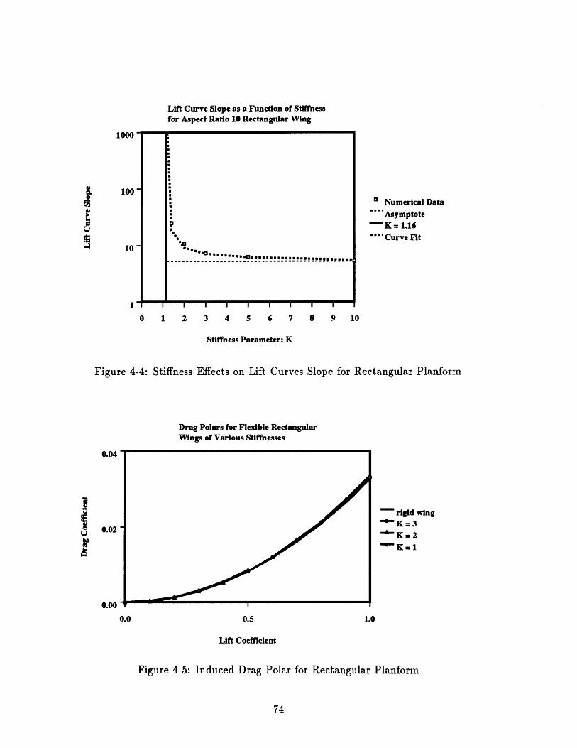
Lift Curve Slope as a Function of Stiffnessfor Aspect Ratio 10 Rectangular Wing
***.,
1000
10
10
* Numerical Data
.. AsymptoteK = 1.16
... ' Curve Fit
0 1 2 3 4 5 6 7 8 9 10
Stiffness Parameter: K
Figure 4-4: Stiffness Effects on Lift Curves Slope for Rectangular Planform
Drag Polars for Flexible RectangularWings of Various Stiffnesses
rigid wingK =3K = 2
-wK= 1
Lift Coefficient
Figure 4-5: Induced Drag Polar for Rectangular Planform
I I I I I I I I
0.04
o 0.02
0.00

4.3 Analysis of Ideal Tapered Wings
The theory that is discussed in Section 2.4.1 describes the performance of high
aspect ratio elliptically loaded flexible wings that are modeled as two-dimensional
plates at every point along the span and boundary conditions right at the leading and
trailing edge of the wing. This theory should also offer insight into the performance
of wings that are nearly elliptically loaded. To verify this theory, a numerical analysis
is performed of several tapered flexible wing planforms. The results of this numerical
analysis are compared to the elliptic theory to show its accuracy for wings that are
not high aspect ratio elliptical wings.
4.3.1 Tapered Wing Planforms
The tapered planforms that are studied here have a very simple geometry. The
planform is trapezoidal with the tip chord equal to one half of the root chord. This
taper ratio is shown by Glauert [4] to give a close approximation to elliptic span
loading. The leading edge is swept back and the trailing edge is swept forward as
shown in Figure 4-6. The 70% chord line is perpendicular to the root chord (this is
important for comparison to the case where the axis of rotation of the trailing edge
spar is placed on this line).
The tapered planforms are used for several reasons. The leading and trailing
edges are straight allowing easy enforcement of the leading and trailing edge boundary
conditions. In the case where the spar boundary conditions are used, the locations
of the spars relative to the local chord is constant along the span of the wing and
the spars are straight. The value of the stiffness parameter, when corrected for axle
placement is also constant over the span. There is a good amount of prior work on
tapered planforms that can be used for comparison.
The lift curve slope for rigid tapered planforms are known from the prior work of
Glauert [4]. Thus, it is easy to compare the lift curves for flexible wings to those for
rigid wings with the same planform. For the case of rigid wings, the lift curve slope of
the tapered wing compared to the elliptic wing is shown for a range of aspect ratios

~5 ~ .st~Jsf ~I~ ~~~" t" ~j~I I ::~:~:~:~:~:~:~::~t~2~S~ ~i
w\\" h:ffl
Trailing EdgeBoundary Condition
Leading EdgeBoundary Condition
Trailing EdgeSpar Region
Flexible Region
Leading EdgeSpar Region
Figure 4-6: Typical Tapered Flexible Wing Model
in Figure 4-7.
The lift curve slope for the family of tapered flexible wings depends on the value
of the stiffness parameter of the wing as well as the aspect ratio. For a given aspect
ratio the lift curve slope increases as the stiffness decreases until the lift curve becomes
completely vertical. The value of the stiffness parameter where this occurs is defined
to be the critical stiffness of the wing and depends on the aspect ratio of the wing.
For values of the stiffness parameter less than the critical stiffness, the lift curve slope
becomes negative.
To determine the effect of aspect ratio on the critical stiffness, Kcrit, the tapered
planforms are modeled without the spar section such that the boundary conditions are
enforced at the leading and trailing edges. The plate is modeled as a uniform isotropic
linearly elastic material. The plate stiffness in the chordwise direction is constant
(constant thickness). The thickness in the spanwise direction is proportional to the
~I7r
"'"'.vir
~w
5,~~~j.5~ I ::::::::~:~:S~:i L ::~:::::
t~t~ ~~i~:~:::::jli:-~ ~
~ 2:c ~i ~j~ tt~s rs~ti
:~ tt~ ~r.~~ :ox:so~ ~~i 5:s~tzz~ ~ -~ ~~ ~i~ ~f~s~:si.5 i t~ ~ ".
I
t:~: ~ :::: : : ~ ~~.... sy
5555~; ~;::::::: :s~"" ~j2.~:~:~::."~:::::~j
~str ~
:~:~::~::~:~:~:~:~:~:::x~f~: ~
r
ss"I I I I I Itoslu:o:~
~1\1 I I I I~f~~x t:~
~rl I I I its:::.~l~E:
t I t I
------- - -- ---------- ~~-~~~~~~~-
j/1
""
~~6~~
~~

Comparison of Elliptic and Tapered Planforms
8
-* *Tapered
Planform4 "'Elliptic Plantorm
- - 2-D slope
2
0 10 20 30 40 50
Aspect Ratio
Figure 4-7: Lift Curve Slopes for Tapered Planforms of Various Aspect Ratio
local chord of the wing such that the local value of the stiffness parameter is constant
over the span. The leading and trailing edges of the wing are simply supported such
that the x and z displacement of the leading edge is constrained and the z displacement
of the trailing edge is constrained (the y displacement is also constrained at the root).
The root and tip of the wing are free from supports.
A series of such ideally modeled flexible wings with varying aspect ratios are tested
to find their critical stiffness, Kc;t. The theoretical K,,ai is given by Equation 2.15.
This theory was developed for elliptically loaded planforms with no structural in-
teraction between spanwise locations. There should be correction to this theory for
non-elliptic distributions and real plates where there is interaction in the spanwise
direction. As described in Section 2.4.1, the camber distribution depends to a large
degree on the aspect ratio. The bending of the plate at the tip of a low aspect ratio
wing will be much more affected by the root bending loads that a high aspect ratio
wing.

4.3.2 Numerical Convergence of Tapered Planform
As a check to prove that the numerical model is appropriate for this planform,
the convergence rate of the numerical method is checked. As shown in Figure 4-8,
the change in the shape of the wing as measured by the average nodal displacement
decays very quickly. The shape of the wing converges in well under 20 iterations.
Once again the convergence rate depends on the stiffness of the wing, but even for
wings with a stiffness less than the critical stiffness, the convergence is good.
AR 6 Ideal Tapered Planform:RMS dz Error Convergence
lx1 "2
1x10⁻¹
1x10⁻⁴
lxl0 "6
1x10⁻⁷
1xi10.
0 2 4 6 8
Iteration
K=3K=2
- K=1.5K=1
10 12 14 16
Figure 4-8: Convergence Rate for Tapered Planform
As the nodal displacements converge to a final steady state shape, the angle
of attack of the wing also converges. Once again, the angle of attack of the wing
converges to within 0.0001 degrees for a RMS error an the order of 10-6 to 10-7. The
convergence of the angle of attack is shown in Figure 4-9.

AR 6 Ideal Tapered Planform:Angle of Attack Convergence
-2 1
0 2 4 6 8 10 12 14
Iteration
Figure 4-9: Convergence Rate for Tapered Planform
4.3.3 Linearity of Lift Curve
The lift curves for a flexible tapered wing of aspect ratio 6 over a range of flexibili-
ties are shown in Figure 4-10. Using the statistical analysis described in Section 4.2.3,
the linearity of each curve can be determined. The very high correlation coefficients
shown in Table 4.2 show that the lift curves generated by the numerical method are
very linear for the tapered planforms. Thus a lift curve can be described simply by
its slope which is determined by a single non-zero lift data point (since the lift curves
all go through the origin).
Table 4.2: Correlation Coefficients for Tapered PlanformK r
Rigid3
1.50.75
0.999960.999900.99990-0.99893
5 5 V
'L IL 5 5 5 U
" K=3K=2K=1.5K=1
16
I- I- I- -r -

Lift Curve:AR 6 Ideal Tapered Planform
1.0
Rigid Wing
0 • K = 1.5" K = .75
0.0
-5 0 S 10 15
Angle Of Attack (degrees)
Figure 4-10: Linearity of Lift Curves for Tapered Planform
4.3.4 Induced Drag Polars
The drag polars for several stiffnesses of the aspect ratio 6 flexible tapered wings
are shown in Figure 4-11. The change in stiffness has a minimal effect on the induced
drag of the wing as can be seen by the similarity among all the curves.
Camber primarily affects the pressure distribution in the chordwise direction.
Since this pressure distribution is the main factor in influencing the boundary layer,
the camber distribution can have large effects on the viscous drag. This drag often
makes a significant contribution to the overall drag on the wing and proper cam-
ber can dramatically improve the viscous and overall drag. However, the computer
programs used in this study do not predict the viscous drag on the wing.
4.3.5 Stiffness Effect on Lift Curve Slope
As the stiffness of the wing changes, the amount of camber for a given lift point and
thus the lift curve slope changes. For very high stiffness when the wing is essentially
rigid, there is little cambering and the lift curve nearly matches that of a rigid wing of

Induced Drag Polar:Ideal Tapered Planform
0.06
Rigd Fin- K 3
K = 1.5
0.02- K .75
0.00 T
0.0 0.5 1.0
Lift Coefficient
Figure 4-11: Similarity of Drag Polars for Tapered Planform
identical planform. As the stiffness decreases, the slope increases until the lift curve
eventually becomes vertical and then negative as seen in Figure 2-3. The critical
stiffness, K,-it, of the wing is defined as the point at which the lift curve slope of the
wing becomes completely vertical. Figure 4-12 shows the relationship of the lift curve
slope to the stiffness, K for the ideally constrained tapered wing planform of Aspect
Ratio 5.
As with the rectangular planform, the relationship of lift curve slope to stiffness
for the tapered planform follows an inverse proportional relationship such that
1m c -. (4.9)
K
The slope is again infinite for the critical stiffness and asymptotically approaches the
lift curve slope for the rigid symmetric tapered wing for very high stiffnesses. Thus
the relationship can be given by a curve fit similar to Equation 4.8 of the form
Fm = mriid + . (4.10)
K - Krit
where mrii is the lift curve slope of a rigid wing and F is a proportionality coefficient

Ideal Tapered Wing, AR=5Slope Vs. Stiffness
100
k2 q Flexible WingU' .... Rigid Wing
.10. Curve Fiton... - K = 0.9751
S................. - - Elliptlc Wing
1 I I I
0 1 2 3 4 5
Stiffness
Figure 4-12: Lift Curve Slope as a Function of Stiffness
that depends on the aspect ratio of the wing. This inverse proportionality relationship
fits the data extremely well as shown by the curve fit data in Figure 4-12.
4.3.6 Aspect Ratio Effect on Flexible Wings
The value of the critical stiffness depends on the aspect ratio of the wing. As the
wing aspect ratio goes down, the critical stiffness, Keit, decreases. A relationship is
given by Widnall et. al. in [10] that relates Kit to the aspect ratio of the wing.
This relationship is based on lifting line theory and given in Equation 2.15 where the
airfoil Ke,it = 1.4. This relationship is shown by the theoretical line in Figure 4-13.
The performance shown by the numerical analysis matches the lifting line perfor-
mance prediction curve fairly well. For high aspect ratios, the numerical performance
of the flexible wing shows the same asymptotic behavior of the critical stiffness as the
lifting line theory predicts. For lower aspect ratios, the lift curve slope decreases. For
extremely low aspect ratios, the camber has very little affect on the lift of the wing
and thus the lift curve slope is not affected by the stiffness of the wing. For aspect

Critical Stiffness as a Function of Aspect Ratiofor an Ideal Tapered Wing with No Spars
1.5
1.0 "i fting Line Theoryi - -t 2-D Theory
- Numerical Results0.5
0.0 I
0 10 20
Aspect Ratio
Figure 4-13: Aspect Ratio Effects on Critical Stiffness
ratios below about 1.2, the numerical method would not converge.
The numerical results show a lower critical stiffness for most aspect ratios than the
lifting line theory predicts. This lower Kit is mainly attributable to the difference
in the way the structure is modeled between the lifting line calculations and the
numerical analysis done here. In the lifting line calculations, the camber at any span
station responds only to the local loading and there is no structural stiffness in the
spanwise direction. In the numerical model used here, the structure is modeled as
a real plate such that there is significant interaction in the spanwise direction. This
has a tendency to decrease the camber at the root and increase it near the tip as
compared with the lifting line theory.
In the low aspect ratio range, the critical stiffness calculated from the numerical
method is greater than that from the lifting line theory. For low aspect ratios the
swept leading edge boundary condition acts to change the bending behavior of the
plate. At higher aspect ratios, the bending is nearly cylindrical where for low aspect
ratios the bending is more conic. This effect causes the structure to actually camber
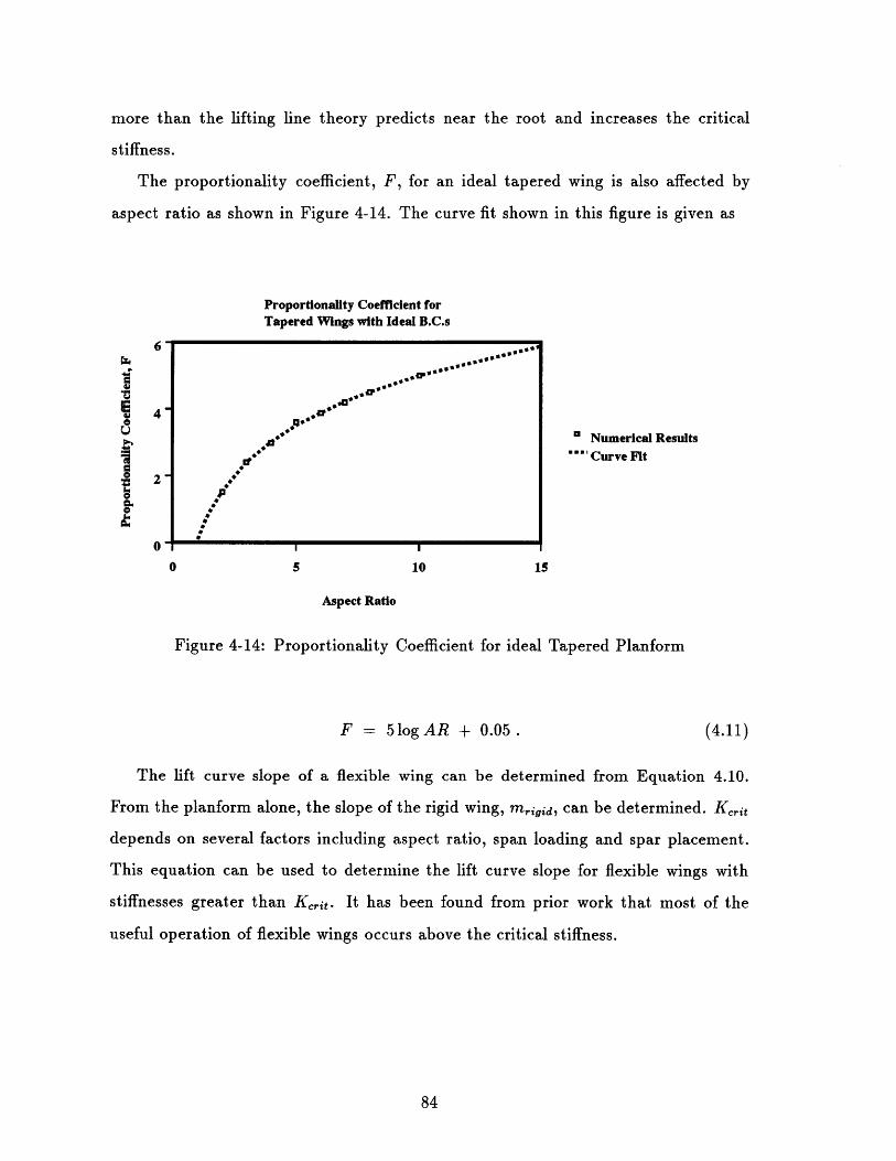
more than the lifting line theory predicts near the root and increases the critical
stiffness.
The proportionality coefficient, F, for an ideal tapered wing is also affected by
aspect ratio as shown in Figure 4-14. The curve fit shown in this figure is given as
Proportionality Coefficient forTapered Wings with Ideal B.C.s
r -u
I I I
0 5 10
" Numerical Results... Curve Fit
Aspect Ratio
Figure 4-14: Proportionality Coefficient for ideal Tapered Planform
F = 5logAR + 0.05. (4.11)
The lift curve slope of a flexible wing can be determined from Equation 4.10.
From the planform alone, the slope of the rigid wing, migid, can be determined. Kcrit
depends on several factors including aspect ratio, span loading and spar placement.
This equation can be used to determine the lift curve slope for flexible wings with
stiffnesses greater than Kcrit. It has been found from prior work that most of the
useful operation of flexible wings occurs above the critical stiffness.

4.3.7 Lift Performance Of Ideal Tapered Wings
The lift coefficient of tapered wings with boundary conditions enforced along the
leading and trailing edges can be expressed as a function of the angle of attack as
27 5 log AR + 0.051 + K- 1.4(1 -. 3
This equation gives the lift coefficient for a wing of given aspect ratio and stiffness.
The comparison of the critical stiffness for the wing with the effective stiffness
for the aspect ratio 5 flexible wing is shown in Appendix A. The comparison to the
stiffness test gives a value for the constant, A. For this wing, A = 0.115 (Widnall
gives the range of A as 0.9 < A < 0.12 in [10]).
The two-dimensional case for these boundary conditions gives A = 0.103 which is
well within the range given by Widnall and very close to A = 0.1 that she gives as
the most likely value for A.
4.4 Analysis of Non-Ideal Tapered Wings
The performance of real wings does not match the ideal performance models that
are characterized in Section 4.3. Two of the major effects on the performance are
caused by the placement of spars and the non-uniform chordwise thickness distribu-
tion of real flexible wings. Real wings cannot be supported by the idealized boundary
conditions of the ideal wings. The thickness of real wings varies along the chord
changing the plate stiffness over the chord. By modifying the models, the effects of
these real wing non-idealities on the wings' performance can be determined.
4.4.1 Spar Boundary Conditions
The idealized supports at the leading and trailing edges that constrain the wings
in the previous section cannot be easily realized for real wings due to the thickness
constraints. All real wings must have spars that are placed where the airfoil is thicker.
The leading edge spar is placed aft of the leading edge in the wing but must be forward

of the 25% chord location in order to allow the wing to camber properly. The trailing
edge spar is placed forward of the trailing edge but must be aft of the 60% chord
location for proper bending. Design tradeoffs for real wings have shown that placing
the spars at the 10% and 70% chord stations gives a reasonable compromise between
the bending behavior and the spar strength.
The spars of each of the wings are modeled as a relatively high modulus isotropic
region of the wing. The spars are designed for very minimal deflection under the
lifting loads by having a modulus that is 7 or 8 orders of magnitude greater than
that of the flexible region. The spar is cantilevered at the root and allowed to rotate
such that the axis of rotation forms a boundary condition for the flexible region. The
spar regions of the wing extends from the axis of rotation to the leading and trailing
edges such that only the region between the spar axes of rotation is allowed to bend
substantially under the loading.
Real wings need to support a substantial spanwise bending loads due to the lift.
This load is supported by the spars or their structural equivalent. The cross-sectional
moment of inertia of the spars is, in general, rather large so as to react the bending
moments. Thus, they are usually placed in the thickest region of the airfoil. For
flexible wings, the spars must be near the leading and trailing edges of the airfoil so
as to provided the proper boundary conditions for the flexible region. Airfoils are
invariably thin near the leading and trailing edges, so the spars need to be rather
large in size to make up for the lack of bending moment of inertia of their cross-
sections. The trailing edge spar, in particular, must be as far forward as possible to
take advantage of the thicker part of the airfoil.
In order to closely model a real wing, the spars in the model have been made rather
large and are placed as close to the center of the airfoil as possible. The trailing edge
spar region makes up the first 10% of the chord of the wing. This location is far
enough from the leading edge as to allow a sizable spar thickness, while still far
enough forward to allow proper bending of the flexible region. The trailing edge spar
makes up the last 30% of the wing at the root and a similar percentage over the span
of the wing. Again, this location allows the spar thickness to be large yet still allows

the flexible region to bend. The wing is made rigid in front of the leading edge axle
and behind the trailing edge axle to keep these regions from deforming under load.
This is particularly important for the trailing edge so as to provide a solid trailing
edge that enforces the Kutta condition. These two regions are shown in Figure 4-21
These realizable spar locations dramatically effect the stiffness of the wing. This
effect comes from several factors. First, the bending region of the plate is shorter in
length effectively increasing its stiffness. Second, the loading between the axles is less
than the total load (some of the load acts in front of the leading edge spar or behind
the trailing edge spar) thus reducing the bending loads on the plate. Finally, the load
that acts in front of the leading edge spar and behind the trailing edge spar act to
"uncamber" the wing due to the adverse moments they apply. All of theses factors
combine to make the plate appear much stiffer than the stiffness parameter indicates.
This effect decreases the value of Krt for a given planform. Using the spar
location correction formula from Widnall et. al. [10],
K,it = 1.3 - 2.6 L.E. Spar _ 2.3(1 - T.E.ar) (4.13)c c
the critical stiffness for an airfoil section with the spars at the 10% and 70% locations
is reduced from 1.4 to 0.35. For an elliptically loaded wing with an aspect ratio of 8,
the finite span correction formula
1.3Kcit win, = Kcrit air oi (1 - 1R) (4.14)
further reduces Kcrit from 0.35 to 0.293. The interaction of the various spanwise
locations of the bending plate reduce Krit further. The numerical analysis for this
tapered wing with an Aspect Ratio of 8 and spars at the 10% and 70% locations gives
K,,it = 0.255.
The lift curve slope for this wing as a function of its stiffness is shown in Figure 4-
15. This Figure shows how the lift curve slope increases as the stiffness decreases. As
the stiffness decreases, the lift curve slope goes up as more of the lift is generated by
camber and less by angle of attack. The slope becomes infinite for the case where all

the lift comes from camber and none from angle of attack. The stiffness where this
occurs is defined to be the critical stiffness of the wing, Kit.
Tapered Planform, AR = 8Slope vs. Stiffness
100
.u.- Flexible WingS""" Rigid Tapered Wing
S....Rigid Elliptic WingS" "K = 0.255
Stiffness ParameterII
I
1 I I I I
0 1 2 3 4 5
Stiffness Parameter
Figure 4-15: Stiffness Parameter Affect on Lift Curve Slope
The relationship between lift curve slope and stiffness follows a similar inverse
relationship as the ideal case. The proportionality coefficient for the tapered planform
with the spar boundary conditions is shown in Figure 4-16. The curve fit that is shown
in that figure gives the functional form for F for this case of a tapered wing with spars
at the 10% and 70% chord positions. This curve fit is given by
F(AR) = log AR + 0.05. (4.15)
Correcting for aspect ratio follows Equation 2.15, but uses the two-dimensional
airfoil Kcrit = 0.35. Thus the curve is similar to the curve for the ideal boundary
conditions, but proportionally lower. This curve along with the numerical data are
presented in Figure 4-17.
The critical stiffness for the wing displays a similar comparison to the lifting line

Proportionality Coefficient forTapered Wings with Spars B.C.s
1A
1.2 00 00....
V 1 .0 ,* *i,"
0.8 ', Experiment
0.6 ""Curve Fit
0.2
0.0
0 5 10 15
Aspect Ratio
Figure 4-16: Aspect Ratio effect on F
prediction as the ideal tapered wing. The critical stiffness falls below the lifting
line prediction at high aspect ratios and for very low aspect ratios are higher than
predicted. However, the vales are close to the lifting line prediction. Thus, a per-
formance curve that utilizes the lifting line prediction gives a good estimate of the
critical stiffness for the wing.
The lift coefficient of tapered wings with spars at the 10% and 70% chord locations,
uniform plate stiffness in the chordwise direction and constant stiffness in the spanwise
direction can be expressed as a function of the angle of attack as
2-r log AR + 0.05CL =( 2 )a (4.16)
1 + A K - 0.35(1- 3)
The comparison of the critical stiffness for the wing with the effective stiffness
for the aspect ratio 5 flexible wing is shown in Appendix A. The comparison to the
stiffness test gives a value for the constant, A. For this wing, A = 0.122 which is
slightly higher than predicted by Widnall et. al. in [10]. The two-dimensional case
for these boundary conditions gives A = 0.104 which is well within the range given
by Widnall and very close to A = 0.1 that she gives as the most likely value for A.

Flexible Tapered WingB.C.s at Axle Locations
0.4
S" Expelment
0.2 Theory--. 2-D Limit
0.0
0 10 20
Aspect Ratio
Figure 4-17: Aspect Ratio Effects on Critical Stiffness for Wing with Spars
4.4.2 Non-Uniform Plate Stiffness
A further correction to the theory involves the non-uniformities in the plate stiff-
ness due to the thickness distribution of the airfoil sections. The wings considered
in the previous sections are modeled as having a uniform plate distribution in the
chordwise direction in the flexible region of the wing. If a constant isotropic material
is used however, the plate stiffness will vary in the chordwise direction as the thickness
varies. This should affect the behavior of the wing slightly.
The plate stiffness, D, for an isotropic plate is given by
E h3
D = (4.17)12(1 - v2)
where E is the modulus of the plate, v is Poisson's ratio and h is the thickness of the
plate. For a NACA 4 digit series airfoil with 15% max thickness (such as a NACA
0015), the thickness distribution is given in [1) as

h(x) = 1.5(0.2969 - 0.126 - 0.3516() + 0 .2 84 3( )3 - 0.1015()). (4.18)
Since the only significant plate bending occurs in the flexible region between the spars,
the average thickness in this region can be determined by taking the integral of the
thickness over this flexible region and dividing by the length of the flexible region,
1 0.7have -= h(x)dx (4.19)
0.6c l=o.1
giving an average thickness of have = 0.132467. The average plate stiffness, D for this
airfoil section is then defined using the average thickness as
E h3Daveave (4.20)
= 12 (1 - v 2 )
giving finally a stiffness for the airfoil section as
DG1/
K = 3ave (4.21)VM 2
where Da,, is the local plate stiffness and c is the local chord of the wing.
For airfoils with this stiffness distribution, The K i correction for axle placement
has not been determined in any of the prior work. However, the correction can
be determined from the effective stiffness test. The results of the two-dimensional
effective stiffness test for spars placed at the 10% and 70% chord locations, as shown
in Appendix A, give an estimate for the airfoil Kc:it = 0.30. Figure 4-18 shows the
effect of non-uniform thickness on the lift curve slope to stiffness relationship.
The lift curve slope for the NACA thickness wing is slightly lower that of the
uniform thickness wing of the same aspect ratio as shown in Figure 4-18. The lift curve
slope again follows the inverse proportionality relationship to the stiffness parameter.
The value of Kent for the wing of finite span again depends on the aspect ratio of
the wing. The comparison of Kcrit for wings of several planforms with both uniform
and NACA thicknesses are shown in Figure 4-19. For this definition of the average

Aspect Ratio 6 Tapered Planform: Comparison ofUniform and Non-Uniform Plate Thickness
100
I:I Uniform Thickness.. K = 0.2310. 10 1 o Non-Uniform Thickness
K = 0.193
IRigid Wing--------------- ------------------ -----------
I1
0 1 2
Stiffness
Figure 4-18: Comparison of Uniform and Non-Uniform Thickness Wings
plate stiffness, the critical stiffnesses for the NACA thickness wings are below those
of the uniform thickness wings.
There is also a correction to F based on the non-uniform plate thickness distribu-
tion. For the aspect ratio 6 wings shown in Figure 4-18, the proportionality coefficient,
F, is decreased from 0.825 to 0.725 for the non-uniform thickness distribution. The
Proportionality Coefficient is affected in a similar way for wings of other aspect ra-
tios. A comparison of The proportionality coefficients for a uniform thickness and a
NACA 0015 thickness distribution are shown in Figure 4-20. For the wing with the
non-uniform thickness distribution, F is given from the curve fit as
F(AR) = 0.868log AR + 0.05 . (4.22)
Thus, the lift coefficient for the flexible wing with NACA thickness distribution is
given by

Critical Stiffness for Tapered Wings with Spar B.C.s:Comparison of Uniform and Non-Uniform Thicknesses
0.4
0.3
... *............ ...
S' -- Uniform Thickness
0.2 9 Non-Uniform Thickness" "'" Uniform Theory
""Non-Uniform Theory
0.1
0.00 5 10 15
Aspect Ratio
Figure 4-19: Effect of Non-Uniform Thickness on Critical Stiffness
27r 0.0868 log AR + 0.05CL =( + )a (4.23)1 + + K - 0.30(1- )
in terms of the aspect ratio and the stiffness parameter of the wing.
subsectionEffective Stiffness Comparison
An effective stiffness test for a tapered wing with an aspect ratio of 5 and the
NACA chordwise thickness distribution is shown in Appendix A. Comparing the
effective stiffness to the numerically calculated critical stiffness gives a value for A =
0.20. This value of A is higher than the A value for the uniform thickness wings.
However, the similar comparison for the two-dimensional airfoil case gave a value for
A = 0.16 indicating that the average plate stiffness for the airfoil may not adequately
model the plate stiffness and would therefore change the stiffness parameter and the
critical stiffness.

Proportionality Coefficient forTapered Wings with Spars B.C.s
1.4
1.2 ...o ***
1.0 PO.
** .o -** I Uniform Thickness0.8 . .o-0.8 .f. ""Curve Fit 1
0.6 o Non-Uniform Thickness
" 0.6 .. .... Curve Fit 2
0.2
0.0 I I
0 5 10 15
Aspect Ratio
Figure 4-20: Effect of Non-Uniform Thickness on Proportionality Coefficient, F
4.5 Tests Involving Sailboard Fin Planforms
Several flexible wing planforms have been developed for sailboard fins. These fins
were developed by Flex Foil Technology Incorporated and are referred to as the Flex
Foil planforms. The analysis of these planforms demonstrates the performance of
real wings. These wings were designed to more closely approximate elliptic loading
than the tapered planforms. The numerical models tested here closely model actual
sailboard fins that have been constructed and sailed.
4.5.1 Sailboard Fin Planforms
One application of flexible wings is in flexible sailboard fins. Several prototypes
of such fins have been developed. These fins present difficult mechanical engineering
problems for their designers. The fins are small yet generate a significant load making
strength of the spars critical. The attachment to the windsurfer itself is also difficult
given the available space inside the board. The fins are much smaller than traditional

windsurfer fins so that they can take advantage of the higher lift coefficients possible
for cambered wings.
The latest prototype fin utilizes carbon fibers in the leading and trailing edge
spars to solve the strength problem. Uni-directional fibers are molded into the lead-
ing and trailing edge regions to provide bending strength. These fibers are tapered
into cylindrical axles at the root which are inserted into holes in the board. These
cylindrical axles are allowed to rotate providing the proper boundary conditions for
the fin. The hole for the trailing edge axle is elongated to allow it to slide. These
same axles react the bending loads on the cantilevered wing due to the lift.
The flexible region between the spars is composed of solid polyurethane rubber.
The modulus of this rubber is carefully controlled to provided the proper stiffness for
the fins allowing them to camber under the lift loads that they generate. This rubber
is molded directly onto the axles providing for a good mechanical joint.
These planforms reflect the design compromises that these real constraints impose
upon flexible wings. The spars are placed at the 10% and 70% chord locations of the
root rather than at the leading and trailing edges of the wing. The leading edge is
straight rather than curved and swept at the root. They also have limited aspect
ratios that reflect the need to react the lift loads by cantilevered supports at the root.
The geometry that is assumed for the wings takes into account the mechanical
aspects of the camber deformation. The leading edge of the wing is swept back at a
small angle but is straight so that the spar can rotate without deforming the wing
out of the x-y plane. The trailing edge spar has a straight leading edge along the
axis of rotation. The trailing edge is curved such that the planform takes on a nearly
elliptical chord distribution. The model is shown in Figure 4-21.
The aerodynamic and structural considerations of the models are based on ac-
cepted wing design principles. The wings were designed with a reasonably high aspect
ratio to minimize the induced drag coefficient. The span however is typically limited
by structural considerations of the spars so the aspect ratio was not set too high. The
shape of the planform is designed such that the lift distribution gives nearly elliptic
loading.

Trailing Edge Boundary Condition
Leading Edge Boundary Condition
Trailing Edge Spar Region
Flexible Region
Leading Edge Spar Region
Figure 4-21: Typical Flexible Sailboard Fin Model
The 8 inch Flex Foil planform has a low surface area resulting in a high lift
coefficient at typical operating point. The surface area is about half of a standard
windsurfer fin. The higher lift coefficient takes advantage of the higher lift capabilities
of the wing due to camber. The aspect ratio is moderately high for good induced
drag performance.
The 10 inch planform has a larger surface area and higher aspect ratio than the
8 inch planform. This results in a lower operating lift coefficient than the 8 inch
planform but better induced drag performance. The surface area is still significantly
lower than standard fins again taking advantage of the higher lift capabilities of the
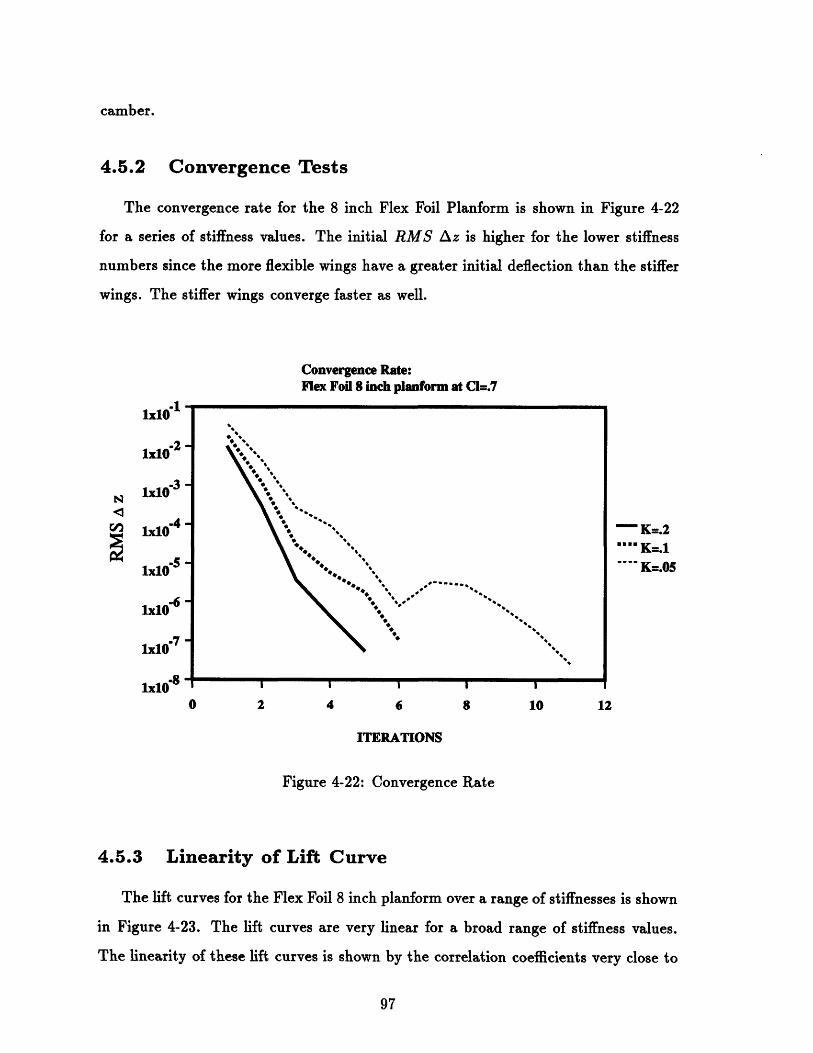
camber.
4.5.2 Convergence Tests
The convergence rate for the 8 inch Flex Foil Planform is shown in Figure 4-22
for a series of stiffness values. The initial RMS Az is higher for the lower stiffness
numbers since the more flexible wings have a greater initial deflection than the stiffer
wings. The stiffer wings converge faster as well.
Convergence Rate:Flex Foil 8 inch planform at Cl=.7
lxl 1O
1x10- 2 -
lx10-3 -
1x10⁻⁴ -
1x10⁻⁵ -
1x10⁻⁶ -
x107 -lxl0- "
-8 -IxtO
U
I I 1 I
2 4 6 8 10
- K=.2""" K=.1
.. K=.05
ITERATIONS
Figure 4-22: Convergence Rate
4.5.3 Linearity of Lift Curve
The lift curves for the Flex Foil 8 inch planform over a range of stiffnesses is shown
in Figure 4-23. The lift curves are very linear for a broad range of stiffness values.
The linearity of these lift curves is shown by the correlation coefficients very close to
.
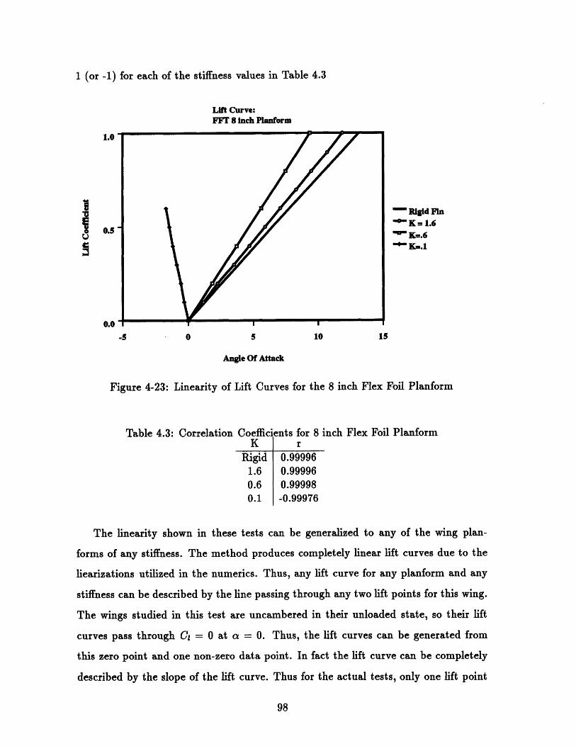
1 (or -1) for each of the stiffness values in Table 4.3
Lift Curve:FFT 8 inch Planform
1.0
SRigid FinK = 1.6
0.5 - K=.6=K=.1
0.0
-5 0 5 10 15
Angle Of Attack
Figure 4-23: Linearity of Lift Curves for the 8 inch Flex Foil Planform
Table 4.3: Correlation Coefficients for 8 inch Flex Foil PlanformK r
Rigid 0.999961.6 0.999960.6 0.999980.1 -0.99976
The linearity shown in these tests can be generalized to any of the wing plan-
forms of any stiffness. The method produces completely linear lift curves due to the
liearizations utilized in the numerics. Thus, any lift curve for any planform and any
stiffness can be described by the line passing through any two lift points for this wing.
The wings studied in this test are uncambered in their unloaded state, so their lift
curves pass through C, = 0 at a = 0. Thus, the lift curves can be generated from
this zero point and one non-zero data point. In fact the lift curve can be completely
described by the slope of the lift curve. Thus for the actual tests, only one lift point

is generated.
4.5.4 Performance of 8 Inch Flex Foil Wing
The lift curve slope to stiffness relationship for the 8 inch Flex Foil Planform is
shown in Figure 4-24. The data follows the inverse relationship shown for the tapered
wings. Thus, the lift curve slope is given by
The curve fit shown in this
and Krit = 0.18. Thus the
Fm = mrigid + . (4.24)
K - Kcit
figure follows this equation with m,igd = 4.345, F = 0.7
lift curve slope for this fin is
0.7m = 4.345 +
K - 0.18(4.25)
8 Inch Flex Foil Planform:Slope vs. Stiffness
100
* Flexible Wing*.. Rlgd Wing-Curve Fit
... Elliptic Wing- - K = .173
0 1
Stiffness
Figure 4-24: Performance Curve for 8 inch Flex Foil Planform
The results of the effective stiffness test for this planform are shown in Appendix A.

The comparison of the critical stiffness calculated numerically and the effective stiff-
ness gives A = 0.194. This is close to A for the NACA thickness tapered wing which
is 0.199.
4.5.5 Performance of 10 Inch Flex Foil Wing
The performance of the 10 inch planform is shown in Figure 4-25. For this wing,
Kcit = 0.173, F = 0.67 and the rigid wing lift curve slope is migid = 4.636. Thus
the lift curve slope for the fin is given as
0.67m = 4.636 + 0.67
K - 0.173(4.26)
8 inch Flex Foil Planform:Slope vs. Stiffness
100
10 -
* Flexible Wing' Rigid Wing
- Curve Fit- Elliptic Wing- - K=.18
I I .I
0 1 2
Stiffness
Figure 4-25: Performance Curve for 10 inch Flex Foil Planform
The results of the effective stiffness test for this planform are shown in Appendix A.
The comparison of the critical stiffness calculated numerically and the effective stiff-
ness gives A = 0.203. This is close to A for the NACA thickness tapered wing which
is 0.199 as well as that for the 8 inch sailboard fin which is 0.194.
100
............................nim
n i
I

4.5.6 Critical Speed for 10 inch Fin
For the case of a wing that has been constructed of a particular material, the
critical stiffness is related to a critical flow dynamic pressure. Since the plate stiff-
ness, D, is fixed by the material properties of the wing, changes in the stiffness are
related only to changes in the speed of the flow. Thus for a wing with fixed material
properties, it is often useful to discuss the critical speed of the wing rather than the
critical stiffness.
For the case of the 10 inch fin, a relationship between the flow speed and the lift
curve slope can be determined. The modulus of the flexible material for this case is
4000psi and the airfoil is a 15% thick NACA section. The fin is operating in water. As
can be seen in Figure 4-26, the slope of the lift curve increases as the speed increases
until the wing reaches it's critical speed of approximately 30 knots.
Lift Curve Slope as A Function of Speed:10 inch Flex Foil Planform, E=4000
100
./ " Numerical Results10 Curve Fit
-" Critical Speed
0 10 20 30 40
Free Stream Velocity (knots)
Figure 4-26: Critical Speed for 10 inch Flex Foil Planform
101

Chapter 5
Conclusions and
Recommendations
The numerical analysis shown in Chapter 4 give the details on the performance of
flexible wings. These curves can be unified into a concise set of performance curves
that adequately describe the behavior of flexible wings. The following sections outline
the results of the analysis in a simple set of performance equations.
5.1 Performance Characteristics of Flexible Wings
The results of the numerical analysis of flexible wings give a good indication of
how they perform. The stability of the method and the quick convergence indicate the
stability of real flexible wings and their response rate to changing operating points.
The actual data shows how a flexible wing behaves at certain operating points.
5.1.1 Camber Stability
The quick convergence of the method indicates a strong stability of the camber of
real flexible wings. As the wing changes shape, the loading quickly responds to the
new shape. The numerical loading changes very little between iterations. The real
loading acts in a similar way minimizing the dynamics of the structure and leading
quickly to the final solution. The final camber shape is very stable for operation
102

above the critical stiffness.
5.1.2 Lift Performance
The lift coefficient for a particular wing is determined by the aspect ratio of the
wing, its planform shape, its stiffness and its angle of attack. These parameters can
be combined into a single equation for elliptically loaded wings:
27r FCL =( 2 + 1.3 ) (5.1)1 + - K - Kcrit airoiz(1 - 1)
where AR is the aspect ratio of the wing, K is the stiffness of the the wing, a is the
angle of attack and CL is the lift coefficient as described earlier. Kcit airfoil depends on
the axle locations and the stiffness distribution along the chord. The proportionality
coefficient, F, also depends on the Aspect Ratio of the wing and the spar placement.
For the case of the tapered wing ideally constrained at the leading and trailing
edges, F is given from a curve fit of the data as
F = 5 log AR + 0.05. (5.2)
Moving the spars to the 10% and 70% chord points changes F to
F = logAR + 0.05. (5.3)
For the flexible wings, with the non,uniform thickness distribution, and the spars at
the 10% and 70% chord locations, F is given as
F = 0.868 log AR + 0.05. (5.4)
This equation is valid for nearly elliptically loaded wings as well. The more non-
elliptic the span loading of the wing is, the further from the predicted lift the actual
lift will be.
This equation shows the inverse relationship between the lift curve slope and the
stiffness of the wing. For a given aspect ratio, the relationship of the lift coefficient,
103

CL, and angle of attack,a, depends only on the stiffness, K in an inverse proportion-
ality.
The proportionality coefficient gives an indication of the sensitivity of the lift
curve slope to changes in the stiffness of the wing. The optimal drag performance
of flexible wings has been experimentally determined to occur for a lift curve slope
around 3 times greater than the rigid wing slope. The magnitude of F for the wing
gives an idea of how close the design speed is to the critical speed. Low values of
F indicate a sharp upturn in the lift curve slope near the critical stiffness and less
difference between the optimal and critical stiffnesses. Larger values of F indicate a
more gradual increase in the slope near critical and thus more of a difference between
the optimal and critical stiffnesses.
The magnitude of F also indicates the range of near optimal stiffness. The flatter
the slope to stiffness curve near the optimal stiffness, the wider the range of stiffnesses
will result in near optimal performance. Larger F values give larger range of near
optimal performance. Since F increases with the aspect ratio, the higher aspect ratio
wings have a larger range of near optimal stiffnesses.
5.1.3 Angle of Attack
In order to avoid the aeroelastic divergence at K,,rt, the numerical program for this
study sets the lift coefficient and determines the angle of attack rather than the other
way around. Although this is the reverse of the way wind tunnel experiments are
performed, it is a valid method for analysis. However, the primary resulting equation
given above, is monotonic allowing it to be inverted so that the more standard CL, a
formulation can be used. This inverse relationship is simply
CLa ( K - K , - )) (5.5)
This is simply a rewritten form of Equation 5.1. This form is included since the
numerical methodology that is used to gather the data, takes the lift coefficient as
the input and determines the angle of attack. This form avoids the singularity at
104

the critical stiffness, Kcit. This form can even obtain the negative angles of attack
that occur for stiffness values lower than Kcit (although there is very little numerical
verification of this range of stiffnesses).
5.1.4 Variation of Parameters with Planform Type
The performance curves that have been generated for the tapered wing planforms
can be used to predict the performance of a more general planform. However, the
accuracy of the predictions depends on how closely the planform of the real wing is to
the tapered model. In the case of the flexible sailboard fins, the trailing edge of the
wing is not straight so that the load is closer to an elliptic distribution. However, the
curve of the trailing edge also changes the positions of the spar rotation axes relative
to the local chord. Near the midspan of the wing, the trailing edge spar makes up a
larger percentage of the local chord than it does near the tip or root. The value of
K,,it and F are both highly dependent on the placement of the boundary conditions.
Thus, the values of Kit and F that are predicted by the performance curves are not
extremely accurate.
However, the effective stiffness test gives a very good prediction of the critical
stiffness. The value of A for the tapered planform with the NACA thickness distri-
bution is very close to the value of A for the sailboard fin planforms for the same
thickness distribution. Thus, if the value of A for the tapered planform is used to
predict Kit based on the effective stiffness test for the sailboard fin planforms, the
predicted Kerits very closely match the Keit calculated numerically.
5.1.5 Low Aspect Ratio Performance
Flexible wings do not perform well at very low aspect ratios. At low aspect ratios
the loading due to camber is not positive over the chord but rather dips negative over
the half of the chord loser to the leading edge. This not only does not provide lift,
but also does not support the camber that causes it. Thus the flexible chordline will
be unstable and the benefits of camber will not be achieved.
105

Lifting line theory suggests a flexible wing with an aspect ratio less than 1.3 can
not achieve any significant performance advantages over a rigid wing. Below 1.3, the
wing loading due to pure camber should not support that camber. For higher values
of the stiffness parameter, the lift curve does increase slightly over the rigid wing, but
the wing becomes unstable before reaching critical stiffness. For loadings due mainly
to angle of attack and only partially to camber, the leading edge loads tend to offset
the negative loads due to the camber and the camber is supported by these loads.
However, as the lift curve slope increases, this leading edge load due to angle of attack
decreases and the chord line becomes unstable. Thus the wing does not have a well
defined critical stiffness nor useful operation at low angles of attack.
The numerical analysis tends to confirm this idea, although the aspect ratio where
it occurs tends to be slightly lower than predicted by lifting line theory. A wing with
an aspect ratio of 1.2 had a converged solution at zero angle of attack, indicating the
critical stiffness for the wing and thus that the aspect ratio where wings no longer
show the full range of behavior is actually lower than 1.2. However, in this aspect
ratio range, the numerical method converges very slowly, indicating that the stability
is weak. A numerical analysis for an ideal wing of aspect ratio 1 could not arrive at
a converged solution for an angle of attack of zero.
Low aspect ratio flexible wings have very low proportionality coefficients F. The
low value for F indicates that the range of stiffness parameter values where substantial
benefits can be derived from camber is small. Thus the difference between the optimal
operating stiffness parameter value and the critical stiffness is small.
5.1.6 Drag Performance
The numerical analysis used in this study to determine the performance of flexible
wings is only capable of determining the induced drag on the wing. The camber of the
wing does not affect the induced drag significantly since the induced drag is simply
a function of the span loading which varies very little as the camber changes. For an
elliptically loaded wing, the induced drag is simply a function of the lift coefficient
and the aspect ratio of the wing.
106
CDi - (5.6)r AR
For non-elliptically loaded wings, the induced drag follows the same form as in
Equation 5.6, but is slightly modified to account for the non-ellipticality with a plan-
form efficiency coefficient, e.
CDi - L (5.7)7r AR e
This efficiency coefficient is a function of the shape of the span loading of the wing.
For an elliptically loaded wing, it is one, and for any other wing it is less than one.
In general, this coefficient is rather close to one for most planforms. The tapered
planforms studied here have an efficiency coefficient on the order of 0.8 to 0.9.
The span loading of a flexible wing does not typically change significantly as the
stiffness changes. This is mainly due to the cambering behavior of the wing. Since
the camber at any spanwise location of the wing is not only affected by the loading
at that point, but the overall plate bending induced by the total loading, the camber
tends to be more evenly distributed than the span loading. Thus, at the tip where
the load is low, the camber is greater than the two-dimensional plate theory would
predict for that airfoil cross-section. Similarly, at the root, where the loading is high,
the camber tends to be lower than the two-dimensional plate theory would predict.
This camber distribution tends to distort the ellipticality of the loading by decreasing
the load at the root and increasing it near the tip. Thus, the efficiency coefficient for
the cambered wing remains relatively close to that of the rigid wing and the induced
drag polar does not change significantly from that of the rigid wing. This is seen for
the case of the tapered planforms in Figure 4-5 and Figure 4-11.
In general, for nearly elliptically loaded wings, the induced drag for the wing
depends only on the planform and the lift coefficient only. Thus, the lift to induced
drag ratio for a flexible wing is nearly constant for constant lift no matter what the
flexibility or camber of the wing.
The camber does, in general, have a significant impact on the viscous drag of
107

the wing. The numerical analysis utilized in this study cannot determine the viscous
drag effects on the wing and thus cannot determine the effect of flexibility on the
viscous drag. However, once the steady state camber has been determined from this
method, and a thickness distribution chosen, the viscous drag of the airfoils or the
entire wing can be determined by utilizing other numerical analyses such as XFOIL
mentioned earlier. The results of the analysis described in Section 2.3 give the optimal
performance for a flexible airfoil. This minimum drag occurs when about 3/4 of the
lift comes from camber and 1/4 from angle of attack. This should hold true for the
airfoil sections of a flexible wing as well.
5.2 Design of Flexible Wings
The results of this study give a good indication of the performance characteristics
of flexible wings. The results can be used by aerodynamic designers that wish to
utilize flexible wings in their vehicle designs.
5.2.1 Steady Load Lifting Surfaces
Flexible wings can be applied to the steady lifting surfaces. However, in order
for these wings to have an advantage over standard fixed geometry wings, the range
of operating lift should be large. One example of a situation where this occurs is
in the keels of sailboats or the fin on a windsurfer. The lift requirement for both of
these devices is relatively constant in magnitude, but switches direction as the craft
"tacks" or "jibes" from one direction of travel to another. In this case, the camber
response of the flexible wing can switch direction as the direction of loading on the
keel changes.
In order to properly design a keel of fin to perform at an optimal level for such
an application, the designer must first understand the operating requirements of the
craft such as speed and lift. A planform should be chosen that can generate high
lift coefficients (0.5 to 0.8) for these operating requirements. The aspect ratio of the
wing is often chosen due to structural constraints of the spars or depth requirements
108

of the keel itself. The spar placement is also determined by structural constraints.
The viscous analysis shown in Section 2.3 indicates that for an optimal lift to
drag ratio occurs for a lift curve slope around three times that of a rigid wing for
Reynolds Numbers on the order of 10'. By performing a similar viscous drag analysis
for the design operating point, the designer can determine a lift curve slope that
maximizes the lift to drag ratio at the operating lift coefficients. The value of the
stiffness parameter of the wing can be determined from the slope using some of the
performance curves in this study. Finally, the material properties of the wing such as
the modulus, can be determined from the stiffness and the operating point through
the equations presented above.
5.2.2 Control Surfaces
Control surfaces are often required to operate over a wide range of lift require-
ments. Flexible wings can be used to enhance the performance of these surfaces
by lowering the drag associated with the control actions and improving the control
authority of the surface. By adding camber to the surface as the lift need goes up
(or negative camber for negative lifts) the control surface can have a much greater
range of lift outputs than a fixed geometry surface. This allows the designer to chose a
lower surface area planform (with an associated lower drag) or to have greater control
authority with the same planform as the rigid control surface.
The passive nature of the camber response allows the operator to achieve these
advantages without the added complexity of mechanical actuators or other active
shaping devices. The automatic response also allows keeps the surface in an optimal
configuration through quick maneuvering. The lower drag associated with such ma-
neuvers through the use of the flexible wings should be an advantage to nearly all
vehicles. This device could be applied to the elevators or tail surfaces of aircraft as
well as the rudders of sailboats.
The lift curve slope for control surfaces represents the control gain of the system.
The designer can tailor the gain of the system by selecting the proper wing stiffness
to achieve the desired lift curve slope. However, the designer should avoid the critical
109
stiffness, where the gain becomes infinite and the control forces can no longer be
commanded. In most cases the design will provide lowest drag far enough from the
critical stiffness that this should not pose a problem to the designer.
5.3 Recommendations for Further Study
This study looks at several of the important parameters that govern the behavior of
flexible wings. However, there are several more characteristics of flexible wings that
should be explored in the future. It is also important to verify these performance
characteristics outside of the numerical environment of the program used here by
conducting wind tunnels tests or other experimental tests.
5.3.1 Spar Placement
The spar placement correction given in Equation 2.12 from Widnall, is simply a
curve fit of available 2-D data. This model should be explored more carefully to see
if there is a better formula that could be used. It may also prove an interesting study
to show the effect on the performance of other spar locations.
The spars in the wings in this model are placed in the model such that the pro-
portions of the chord that are in front of, between and behind these spar locations
are roughly constant over the span. It may be interesting to explore cases where
this proportionality is not so constant or even cases where the axes of rotation of the
spars are external to the structure for part of the span. For example, in the case of
the tapered wing, if the leading edge spar axis of rotation were perpendicular to the
root chord, the axis of rotation would be substantially ahead of the leading edge at
the wing tip. The performance of such a wing would be drastically different from the
tapered wings where the axis of rotation is within the structure.
110

5.3.2 Viscous Drag
This study utilized an extremely simplified model that did not include any of the
effects of viscous drag, which is where cambered wings gain most of its performance
advantages. The performance optimization must therefore include these viscous ef-
fects. This could be done by either replacing the vortex lattice with a viscous panel
program or more simply, by post processing the converged result of a numerical pro-
gram similar to the one presented here with a viscous flow solver.
5.3.3 Planforms
This study was mainly concerned with the simple tapered wing planforms. These
planforms are nearly elliptically loaded and thus follow the theory reasonably well.
Further study on other types of planforms with more or less elliptic load distributions
may enhance flexible wing theory.
5.3.4 Non-Uniform Stiffness in the Spanwise Direction
The stiffness parameter, K, was considered to be constant over the span of the
wing for these tests. However, better performance may be achieved by varying the
stiffness in the spanwise direction. Making the wing stiffer near the tip or stiffer near
the root may have beneficial or adverse affects on the spanwise camber distribution
and change the performance characteristics.
5.3.5 Other Non-Uniform Chordwise Stiffness Distributions
Two chordwise stiffness distributions were chosen for this study. The uniform
chordwise stiffness distribution gives a good simple model for the flexible wings. The
plate stiffness that accounts for real airfoil thickness distributions gives a good idea
of how the performance curves are modified for non-uniform stiffness distributions.
These are two of only a large number of possible stiffness distributions that can be
utilized.
111

In particular, the chordwise stiffness distribution could be modified to shift the
camber closer to the leading edge or the trailing edge. Although the inviscid results
presented here may not be drastically modified by a change in the stiffness distribu-
tion, a viscous analysis may show a marked performance improvement for a slightly
different stiffness distribution.
There is also an issue of changing the spanwise stiffness distribution. By adding
stiffness near the root or near the tip, it may be possible to modify the span loading of
the wing to make it more elliptical. This would, in general, depend on the particular
planform that is used.
5.3.6 Wind Tunnel Tests
As with other aerodynamic devices, wind tunnel tests can be used to verify or
enhance numerical solutions. It is important to be able to reproduce the performance
of the flexible wings in the wind tunnel to prove the stability and accuracy of the
method.
5.3.7 Shred
One of the primary applications to date is the application to windsurfer fins as
developed by Flex Foil Technology Incorporated. Possibly one of the best ways to see
the benefits of flexible wings is to put one of these fins on your board and go sailing.
The lower drag results in improved speed which any high performance sailor should
feel.
Although these fins are not yet available to the general public, they may soon be
on the market. Until they are, if you see a sailor fly by you on the water and you
can't figure out why he is going so fast, it could be that he is one of the test pilots
for Flex Foil trying out one of their new secret weapons.
112

Appendix A
Effective Stiffness Analysis
The numerical results for a number of effective stiffness tests are presented in this
appendix to show a typical solution. The examples that have been selected and
presented here are not the complete set of analyses, but rather give a few typical
results to demonstrate the methodology of the test. These examples should give the
reader a good idea of the details of the analysis process and allow the reader to more
easily reproduce the results.
A.1 Two-Dimensional Effective Stiffness Tests
The Effective stiffness tests described in Section 2.4.2 can be used to determine
the critical stiffness, K,rit of a two-dimensional flexible airfoil section. The bending
of a infinite plate under an distributed line load gives the load to deflection ratio for
the airfoil. This ratio gives the effective stiffness of the plate
PSe -f . (A.1)
where P is the load per unit span and w is the deflection of the plate at the point of
loading.
The load is applied at the midpoint between the boundary conditions. For these
two-dimensional tests, a unit square plate is loaded with a load of 100 distributed
113

along a line midway between the boundary conditions. The plate has 10 elements
along each edge (11 nodes along each edge). The load is applied to a line spanning
the plate containing 11 nodes. This load is applied in a consistent way by applying a
load of 10 to all 9 interior nodes and a load of 5 to each of the 2 edge nodes. Thus a
total load of 100 is applied to the plate.
The critical stiffness for the airfoils is given from calculations based on the plate
equation
D O4() = p(X). (A.2)
From the definition of the stiffness parameter
DK - (A.3)
q00 ( )3
the critical dynamic pressure is given as
Dqcit = () (A.4)
This value for the critical stiffness is compared to the effective stiffness for the airfoil
giving a value for A as
A = "q (A.5)Sei1
A.1.1 Plate with Ideal Boundary Conditions
The effective stiffness test is used to determine the critical stiffness of an ideal
flexible airfoil. The geometry and boundary conditions for the plate as well as the
consistent nodal loading that is applied are shown in Figure A-1.
The plate used for this test has an elastic modulus E = 3.000 x 10', a Poisson's
ratio v = 0.3 and a thickness h = 0.12. The plate stiffness, D, is given by
E h3
D = 12(1 - 2) (A.6)12(1 - v2)
114

ADINA-IN VERSION 3.0.3, 6 MAY 19932-D Effective Stiffness Test for Ideal Plate
ADINA ORIGINAL
0.09253
XVMIN -0.8944XVMAX 0.4472YVMIN -0.8944YVMAX 0.000
PRESCRIBEDFORCE
TIME 1.000
10.00
U1 U2 U3 81 '2 83
C /--///D -/-///
Figure A-1: Effective Stiffness Test: Ideal B.C.s
For this model, D = 47.5.
The deflection of the plate is shown in Figure A-2. Under the applied load of 100,
the average deflection of the midchord, w, is 0.038 Thus, the effective stiffness, Se, ,
is 2631.
The critical stiffness for an ideally supported airfoil is given as K, it = 1.4. Thus,
the critical dynamic pressure is
(A.7)qeri = Kcrit(j)3
giving a value of q,,t = 271.27
Given Sq, = 2631 from the effective stiffness test, A is calculated to be 0.1031.
115
z
x--

ADINA-PLOT VERSION 4.0.3, 6 MAY 19932-D Effective Stiffness Test for Ideal Plate
ADINA ORIGINAL DEFORMED XVMIN -0.8944 ZLOAD STEP L -.-J XVMAX 0.4472TIME-1.000 0.09253 0.09253 YVMIN -0.8944
YVMAX 0.000 XY
V
- UzU 2 U3 1 2 8 3B //-///C /--///
D -/-///
Figure A-2: Effective Stiffness Test: Ideal B.C.s
A.1.2 Plate with Spar B.C.s and Uniform Thickness
The critical stiffness for the two-dimensional airfoil sections for the wing with the
boundary conditions at the 10% and 70% chord locations can be determined from the
effective stiffness of a plate with these boundary conditions. The plate used for this
test has a modulus of E = 1.000 x 10', a Poisson's ratio of v = 0.3 and a uniform
thickness of h = 0.12 giving a plate stiffness of D = 15.82. The load and boundary
conditions for this effective stiffness test are shown in Figure A-3.
The displacement of the test plate is shown in Figure A-4. The deflection at the
midspan for this test is 0.02878 giving an effective stiffness of Seff = 3475.
For a flexible airfoil with a uniform plate thickness and the spars placed at the
10% and 70% chord positions, the critical airfoil stiffness is given by Widnall et. al.
as Kerit is 0.35. The critical dynamic pressure is then quit = 361.7. Thus, the value
for A for this airfoil is 0.1041.
116

ADINA-IN VERSION 3.0.3, 6 MAY 19932-D Effective Stiffness Test (uniform thickness)
ADINA ORIGINAL XVMIN -0.8944 ZXVMAX 0.4472
0.09253 YVMIN -0.8944YVMAX 0.000 X
Y
PRESCRIBEDFORCE
TIME 1.000
10.00
SU U2 3 818e2 83B //-///C / - - ///D -/-///E --- //B
Figure A-3: Effective Stiffness Test: Spar B.C.s and Uniform Thickness
117

Figure A-4: Effective Stiffness Test: Spar B.C.s and Uniform Thickness
118

A.1.3 Plate with Spar B.C.s and NACA Thickness
The critical stiffness for the two-dimensional airfoil with the boundary conditions
at the 10% and 70% chord locations and the NACA thickness distribution can be
determined from the effective stiffness test. The plate used for this test has a modulus
of E = 1.000 x 10⁵, a Poisson's ratio of v = 0.3 and an average thickness of h =
0.132467 giving an average plate stiffness of D = 21.28. The load and boundary
conditions for this effective stiffness test are shown in Figure A-5.
ADINA-IN VERSION 3.0.3, 6 MAY 19932-D Effective Stiffness Test (NACA thickness)
ADINA ORIGINAL XVMIN -0.8944 ZXVMAX 0.4472
0.09253 YVMIN -0.8944YVMAX 0.000 X
Y
PRESCRIBEDFORCE
TIME 1.000
10.00
U U2 U3 812 83B //-///
D -/-///
Figure A-5: Effective Stiffness Test: Spar B.C.s with NACA Thickness
The displacement of the test plate is shown in Figure A-4. The deflection at the
midspan for this test is 0.01804 giving an effective stiffness of Se11 = 5543.
For a flexible airfoil with a uniform plate thickness and the spars placed at the
10% and 70% chord positions, the critical airfoil stiffness is given as Ke,.i is 0.30. The
critical dynamic pressure is then qcrit = 567.6. Thus, the value for A for this airfoil
is 0.1024.is 0.1024.
119

Figure A-6: Effective Stiffness Test: Spar B.C.s and NACA Thickness
120
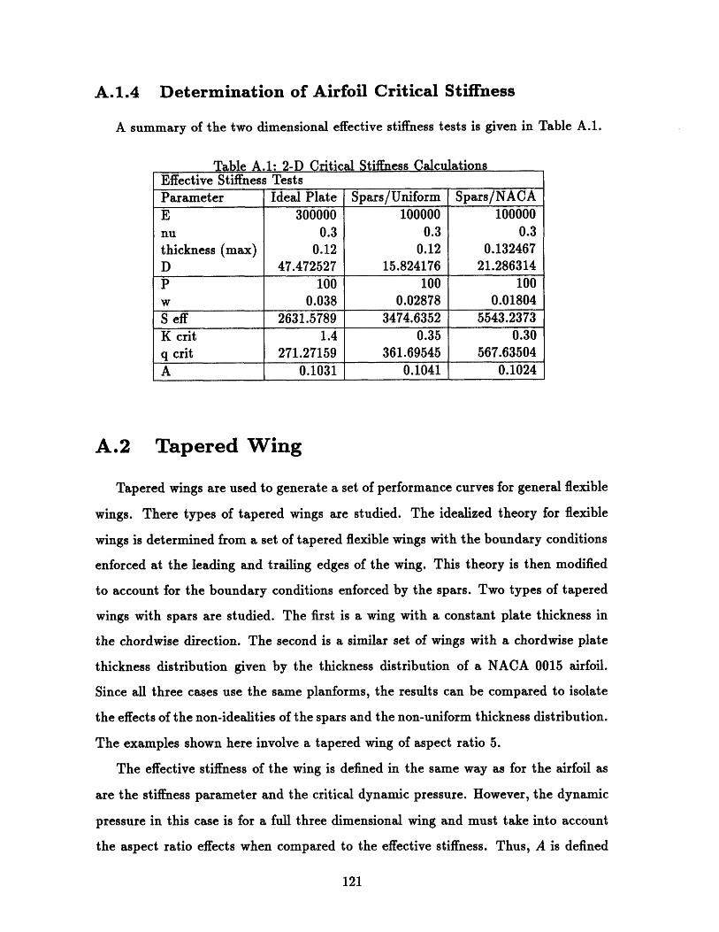
A.1.4 Determination of Airfoil Critical Stiffness
A summary of the two dimensional effective stiffness tests is given in Table A.1.
Table A.1: 2-D Critical Stiffness CalculationsEffective Stiffness TestsParameter Ideal Plate Spars/Uniform Spars/NACAE 300000 100000 100000nu 0.3 0.3 0.3thickness (max) 0.12 0.12 0.132467D 47.472527 15.824176 21.286314P 100 100 100w 0.038 0.02878 0.01804S eff 2631.5789 3474.6352 5543.2373K crit 1.4 0.35 0.30q crit 271.27159 361.69545 567.63504A 0.1031 0.1041 0.1024
A.2 Tapered Wing
Tapered wings are used to generate a set of performance curves for general flexible
wings. There types of tapered wings are studied. The idealized theory for flexible
wings is determined from a set of tapered flexible wings with the boundary conditions
enforced at the leading and trailing edges of the wing. This theory is then modified
to account for the boundary conditions enforced by the spars. Two types of tapered
wings with spars are studied. The first is a wing with a constant plate thickness in
the chordwise direction. The second is a similar set of wings with a chordwise plate
thickness distribution given by the thickness distribution of a NACA 0015 airfoil.
Since all three cases use the same planforms, the results can be compared to isolate
the effects of the non-idealities of the spars and the non-uniform thickness distribution.
The examples shown here involve a tapered wing of aspect ratio 5.
The effective stiffness of the wing is defined in the same way as for the airfoil as
are the stiffness parameter and the critical dynamic pressure. However, the dynamic
pressure in this case is for a full three dimensional wing and must take into account
the aspect ratio effects when compared to the effective stiffness. Thus, A is defined
121

A = qc,.it(1 - ). (A.8)A Seff (A.8)
A.2.1 Ideal Boundary Conditions
The first tapered wing case is the wing with the boundary conditions enforced
at the leading and trailing edge. This case can be compared to the two-dimensional
ideal airfoil so that the effects of aspect ratio alone can be studied. The results of
the effective stiffness test can be compared to the critical stiffness that is obtained
numerically.
ADINA-IN VERSION 3.0.3, 6 MAY 1993Ideal Tapered Wing Effective Stiffness Test
ADINA ORIGINAL XVMIN -0.8944 ZXVMAX 0.5255
0.09792 YVMIN -0.8398YVMAX 0.000 X
PRESCRIBEDFORCE
ETIME 1.000
C I 6.000
U1 U2 U3 8182 83
C /--,,,D -/-///
Figure A-7: Ideal Tapered Wing: Effective Stiffness Test Loading
The wing is loaded as shown in Figure A-7. This loading case is the consistent
nodal loading for P = 32 (load/unit span). The material properties of this wing
are given as E = 1.0 x 10s, v = 0.3. The thickness of the plate is constant in the
122
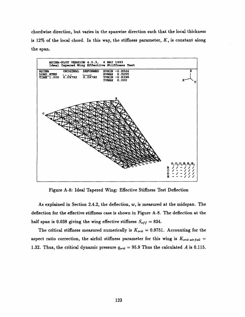
chordwise direction, but varies in the spanwise direction such that the local thickness
is 12% of the local chord. In this way, the stiffness parameter, K, is constant along
the span.
ADINA-PLOT VERSION 4.0.3, 6 MAY 1993Ideal Tapered Wing Effective Stiffness Test
ADINALOAD STEPTIME-1. 000
C ~s
ORIGINAL DEFORMED XVMIN -0.8944LJ I I XVMAX 0.52550.09792 0.09792 YVMIN -0.8398
YVMAX 0.000
3
z
X
U1U2 U3 8182 83
C
Figure A-8: Ideal Tapered Wing: Effective Stiffness Test Deflection
As explained in Section 2.4.2, the deflection, w, is measured at the midspan. The
deflection for the effective stiffness case is shown in Figure A-8. The deflection at the
half span is 0.038 giving the wing effective stiffness Sff = 834.
The critical stiffness measured numerically is Kit = 0.9751. Accounting for the
aspect ratio correction, the airfoil stiffness parameter for this wing is K,,it ir foil =
1.32. Thus, the critical dynamic pressure qrit = 95.9 Thus the calculated A is 0.115.
123

A.2.2 Spar B.C.s and Uniform Thickness
The second tapered wing case is a wing with the boundary conditions enforced at
the 10% and 70% spar locations at the root of the wing. The plate thickness for this
case is uniform in the chordwise direction. The critical stiffness for the airfoil sections
for this wing are given by Equation 2.12 as 0.35.
ADINA-IN VERSION 3.0.3, 6 MAY 1993Tapered Wing Effective Stiffness Test (Uniform Thickness)
ADINA ORIGINAL XVMIN -0.8944 ZXVMAX 0.5255
0.09792 YVMIN -0.8398YVMAX 0.000 X
Y
PRESCRIBEDFORCE
TIME 1.000
6.000
U1 U2 U3 182 3
C /--///D -/-///E
Figure A-9: Ideal Tapered Wing: Effective Stiffness Test Loading
The wing is loaded as shown in Figure A-9. This loading case is the same consistent
nodal loading for P = 32 (load/unit span) as given in the ideal effective stiffness test
described in the previous section. The material properties of this wing are given as
E = 5.0 x 10⁴, v = 0.3. The thickness of the plate varies in the spanwise direction
such that the local thickness is 12% of the local chord.
The deflection for the effective stiffness case is shown in Figure A-10. The de-
flection, w, measured at the midspan is 0.018 giving the wing effective stiffness
Seff = 1769.
124
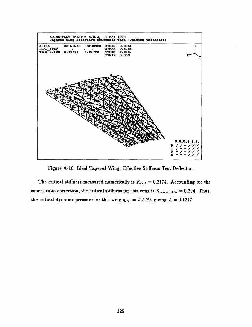
Figure A-10: Ideal Tapered Wing: Effective Stiffness Test Deflection
The critical stiffness measured numerically is K,,it = 0.2174. Accounting for the
aspect ratio correction, the critical stiffness for this wing is Ki airfoil = 0.294. Thus,
the critical dynamic pressure for this wing qit = 215.29, giving A = 0.1217
125

A.2.3 Spar B.C.s and NACA Thickness
The final tapered wing case is also a wing with the boundary conditions enforced
at the 10% and 70% spar locations at the root of the wing. The plate thickness for
this case, however is given by a NACA airfoil thickness distribution in the chordwise
direction. There is no expression in the prior work to estimate the critical stiffness
for the airfoil sections for this wing. However, from the effective stiffness test in
Section A.1.3, the airfoil Kc,it is estimated to be approximately 0.30.
ADINA-IN VERSION 3.0.3, 6 MAY 1993Tapered Wing Effective Stiffness Test (NACA Thickness)
ADINA ORIGINAL XVMIN -0.8944 ZXVMAX 0.5255
0.09792 YVMIN -0.8398YVMAX 0.000 X
PRESCRIBEDFORCE
TIME 1.000
S6.000
C /--///D -/-///
Figure A-11: NACA Tapered Wing: Effective Stiffness Test Load
The wing is loaded as shown in Figure A-9. This loading case is the same consistent
nodal loading for P = 32 (load/unit span) as given in the ideal effective stiffness test
described in the previous section. The material properties of this wing are given as
E = 5.0 x 10⁴, v = 0.3. The thickness of the plate varies in the spanwise direction
such that the local maximum thickness is 15% of the local chord. The thickness in the
chordwise direction between the 10% and 70% chord locations follows Equation 4.18.
126

ADINA-PLOT VERSION 4.0.3, 6 MAY 1993Tapered Wing Effective Stiffness Test (NACA Thickness)
ADINA ORIGINAL DEFORMED XVMIN -0.8944 ZLOAD STEP L . . J XVMAX 0.5255TIME-1.000 0.09792 0.09792 YVMIN -0.8592
YVMAX 0.000 X
Y
5 - UU 3 1 E8,2893
E --- ///
Figure A-12: NACA Tapered Wing: Effective Stiffness Test Deflection
The deflection for the effective stiffness case is shown in Figure A-10. The de-
flection, w, measured at the midspan is 0.019 giving the wing effective stiffness
Sef, = 1686.
The critical stiffness measured numerically is Ke,it = 0.187. Accounting for the
aspect ratio correction, the airfoil stiffness parameter for this wing is K,.t airfoil =
0.253. The critical dynamic pressure, qcrit = 336.54 giving A = 0.1996
127

A.3 Flexible Sailboard Fins
Effective stiffness tests were also performed on the sailboard fins. Rather than the
simple geometry of the tapered wings, these planforms have a chord distribution that
more closely matches an elliptic shape. The chord distribution has been designed to
cause the loading to more closely match an elliptic distribution. The spars are again
placed at the 10% and 70% chord locations at the root and the spars are straight.
However, since the trailing edge is not straight, the local spar axes of rotation do
not lie at the 10% and 70% chord locations. Thus, even though the plate stiffness
is proportional to the cube of the local chord the, change in boundary condition
placement over the span causes the stiffness parameter to vary over the span. The
effective stiffness test allows the complex stiffness distribution of the wing to be
expressed in terms of a single number.
A.3.1 8 inch Flex Foil Fin Planform
The first flexible fin case is the 8 inch flex Foil planform. The Aspect ratio for
this fin is 6.0. The span is 8 inches and the root chord is 3.5 inches.
The fin is loaded as shown in Figure A-13. This is a consistent nodal loading
for P = 10 (pounds/inch). The material properties of this wing are given as E =
5.0 x 10³ psi, v = 0.3. The thickness of the plate varies in the spanwise direction
such that the local maximum thickness is 15% of the local chord. The thickness in
the chordwise direction between the spar locations follows Equation 4.18.
The deflection for the effective stiffness case is shown in Figure A-14. The deflec-
tion, w, measured at the midspan is 0.041 inches giving the wing effective stiffness
Sef = 243psi.
The critical stiffness measured numerically is Kit = 0.180. Accounting for the
aspect ratio correction, the airfoil stiffness parameter for this wing is Kc ait.oil =
0.230. Then, q,it = 47.14psi gives A = 0.194
128

ADINA-IN VERSION 3.0.3, 6 MAY 19938 inch Flex Foil Fin - Effective Stiffness Test
ADINA ORIGINAL XVMIN -3.130 ZXVMAX 2.458
0.3854 YVMIN -3.405YVMAX 0.000 X
Y
PRESCRIBEDFORCE
ETIME 1.000
C
5.000
U1 U 2 U 3 8182 83
B //-///C /--///D -/-///
Figure A-13: 8 inch Flex Foil Fin: Effective Stiffness Test Load
129

ADINA-PLOT VERSION 4.0.3, 6 MAY 19938 inch Flex Foil Fin - Effective Stiffness Test
ADINA ORIGINALLOAD STEP L _JTIME-1.000 0.3854
DEFORMED XVMIN -3.130XVMAX 2.458
0.3854 YVMIN -3.421YVMAX 0.000
u1u2u3ele 2 e3B//-///C /--//!D -/-///E --- //
Figure A-14: 8 inch Flex Foil Fin: Effective Stiffness Test Deflection
130
z
X

A.3.2 10 inch Flex Foil Fin Planform
The 10 inch planform
root chord is 3.7 inches.
has an aspect ratio of 7.36. The span is 10 inches and the
ADINA-IN VERSION 3.0.3, 6 MAY 199310 inch Flex Foil Fin - Effective Stiffness Test
ADINA ORIGINAL XVMIN -3.309 ZXVMAX 3.073
0.4402 YVMIN -4.147YVMAX 0.000 X
PRESCRIBEDFORCE
TIME 1.000
5.000
B //-///C /--///D -/-///E
Figure A-15: 10 inch Flex Foil Fin: Effective Stiffness Test Load
The fin is loaded as shown in Figure A-15. This is a consistent nodal loading
for P = 10 (pounds/inch). The material properties of this wing are given as E =
5.0 x 10³ psi, v = 0.3. The thickness of the plate varies in the spanwise direction
such that the local maximum thickness is 15% of the local chord. The thickness in
the chordwise direction between the spar locations follows Equation 4.18.
The deflection for the effective stiffness case is shown in Figure A-16. The de-
flection, w, measured at the midspan is 0.05 inches giving the wing effective stiffness
S,,f = 200psi.
The critical stiffness measured numerically is Keit = 0.171. Accounting for the
aspect ratio correction, the airfoil stiffness parameter for this wing is K t air oil =
131

Figure A-16: 10 inch Flex Foil Fin: Effective Stiffness Test Deflection
0.388 giving q,,it = 40.6psi and A = 0.203
132

Appendix B
Numerical Analysis
This appendix shows some of the output plots from the numerical analysis. They
are presented to show some examples of the numerical solutions and the steady state
behavior of the flexible wings. Examples are shown for a typical planform for each of
the wing types analyzed in Chapter 4.
Numerical results are shown for several of the interesting operating points of the
flexible wings. The load distribution output plots from the vortex lattice code are
included for the rigid wing loading and critical stiffness loading for each of the example
wings. Output plots from the finite element program showing the wing deflection at
the critical stiffness are also included. These plots are typical of the output from the
computer programs.
B.1 Tapered Wing: Ideal Boundary Conditions
The loading of a rigid tapered wing with aspect ratio of 5 is shown in Figure B-1.
Figure B-2 shows the loading at the critical stiffness for the wing. Since the angle
of attack is nearly zero, all the load is produced by the camber of the wing as is
plainly shown in this figure.
Figure B-2 shows the deflection of the wing at the critical stiffness.
133

RR S TAPEREDALFA = 6.889 Z
CL = 0.500 C
Fi
AR 5 TAPEREDALFA = 0.003 ZCL = 0.515 C
CL = 0.365
CL = 0.470
N Y A CL I 0.514
A ACL = 0.532
1w " wc W 1A'w CL = 0.537
CL = 0.534
1w .YCL = 0.525
f Y-Y e P - X' CL - 0.513
-,w-..- 1w -A-CL = 0.497
/-.-/ -YCL - 0.477
FLEXIBLE HINGSYM1000.0000I = 0.01507 CM = -0.1699
gure B-1: AR 5 Tapered Flexible Wing: Rigid Loading
CL - 0.343
CL - 0.442
CL = 0.539
CL = 0.545
CL = 0.546
CL = 0.545
// CL 0.30.542C I _ CL 0.52353
FLEXIBLE HING: IDEAL B.CSYM1000.00001 CL = 0.01633 CM 51-0.316
Figure B-2: Ideal AR 5 Flexible Wing: Load at KcritFigure B-2: Ideal AR 5 Flexible Wing: Load at Kcrit
134

ADINA-PLOT VERSION 4.0.3, 6 MAY 1993AR 5 Tapered Flexible Wing: Ideal B.C.
ADINA ORIGINAL DEFORMEDLOAD STEP L - .TIME-1.000 0.09792 0.09792
XVMIN -0.8944XVMAX 0.5255YVMIN -0.8569YVMAX 0.000
z
C /--///D -/-///E ///
Figure B-3: Ideal AR 5 Flexible Wing: Camber at Kcritlabelapp:ideal5-w
135

B.2 Aspect Ratio 5 Tapered Wing: Spar Bound-
ary Conditions
The rigid loading for this wing planform is shown in Figure B-1. The bound-
ary conditions and thickness distributions have no affect on the loading of the rigid
wing. Thus, this rigid planform is identical to the tapered wing with ideal boundary
conditions for the rigid case.
B.2.1 Aspect Ratio 5 Tapered Wing: Uniform Thickness
Figure B-4 shows the loading at the critical stiffness for the wing. Since the angle
of attack is nearly zero, all the load is produced by the camber of the wing as is
plainly shown in this figure.
CL a 0.305
-CL 0. 380
CL - O.A10
-WCL - 0.422
CL -0.397
CL -0.3811
AR 5 FLEXIBLE NING: SPAR B.C.ALFA = 0.003 ZSTl1000.000CL = 0.400 CDI = 0.00974 CM = -0.0098
Figure B-4: Uniform thickness AR 5 Flexible Wing: Load at Kcrit
136

ADINA-PLOT VERSION 4.0.3, 6 MAY 1993AR 5 Flexible Wing: Uniform Thickness
ADINA ORIGINALLOAD STEP L - JTIME-1.000 0.09792
DEFORMED XVMIN -0.89440- , XVMAX 0.52550.09792 YVMIN -0.8569
YVMAX 0.000
z
Y
U1 U2 U 3 182 3B //-///C -- //D -/-///E - - - J//
Figure B-5: Uniform Thickness AR 5 Flexible Wing: Camber at Kcrit
B.2.2 Aspect Ratio 5 Wing: NACA Thickness
For the NACA stiffness distribution, the loading is slightly different near K,,it.
than the uniform stiffness.
Figure B-7 shows the deflection for this wing.
137
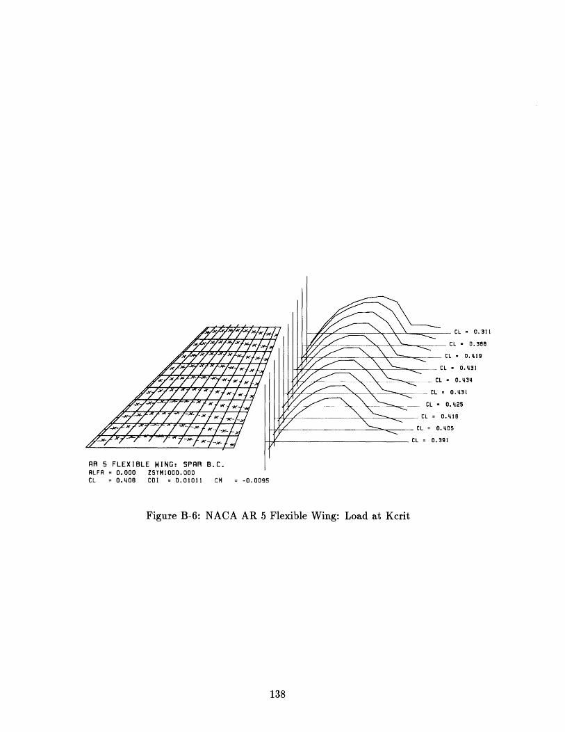
,,
-
-w-
-x
PR 5 FLEXIBLE HING: SPAR B.C.ALFA = 0.000 ZSTM1000.000CL = 0.408 CDI = 0.01011 CM = -0.0095
CL = 0.311
CL = 0.38
CL = 0.419
CL - 0.431
CL - 0.434
Y CL - 0. 431
CL = 0. 425
CL = 0.416
CL = 0.405
CL = 0.391
Figure B-6: NACA AR 5 Flexible Wing: Load at Kcrit
138
-KrX% K
r~x-/x~x ~fx-

Figure B-7: NACA AR 5 Flexible Wing: Camber at Kcrit
139
ADINA-PLOT VERSION 4.0.3, 6 MAY 1993AR 5 Flexible Tapered Wing: NACA Thickness
ADINA ORIGINAL DEFORMED XVMIN -0.8944 ZLOAD STEP L__ J _ XVMAX 0.5255TIME-1.000 0.09792 0.09792 YVMIN -0.8571
YVMAX 0.000 X
1 U2U3e818283cB //-///C / - - // /
B.3 Flexible Sailboard Fins
Results are shown for both Flex Foil planforms as the deflection behavior of these
planforms is quite unique. Giver the non-uniformity in the stiffness parameter in
the spanwise direction, the camber response takes on a unique shape that should be
shown.
B.3.1 8 inch Fin Planform
Plots for the 8 inch planform are included to show the rigid wing loading as well
as the loading at the critical stiffness. The camber response near the tip of the wing is
higher than in the tapered wing examples due to the large percentage of the chord of
the flexible region near the tip. This causes the tip to camber more than it normally
would, and distorts the elliptic loading.
140

CL = 0.357
CL = 0. 38
SLCL = 0.05lokIw aCL 0.413
FLEXIBLE -IN FLEXCL FOIL 17
LF = 5.182 SYCL .000.0018
CLCL = 0.00 CDI 0.00820 CM = -0.290.8Figure B-8: 8 inch Flex Foil Planform: InitCLa Load
ww. , / CL m 0.412SCL - O.409
-A" CL - 0.405
"-X- CL , 0.3!92
74.%-/ X 7 w CL = 0. 385
FLEXIBLE KING: FLEX FOIL 8"ALFA - 5.182 ZSrM1000.000CL = 0.400 C01 x 0.00820 CH = -o.2918
Figure B-8: 8 inch Flex Foil Planform: Initial Load
141

**/2 /r ,* /-/ ,-1 "Iw-.I7-Ttyw*W77K
,//7 /"-/ / //7"/7. /, /I /
-" -/- /
FLEXIBLE HING: FLEX FOIL 8"ALFA = -0.000 ZSYMI000.000CL = 0.502 CDI = 0.01308 CM = -0.4553
Figure B-9: 8 inch Flex Foil Planform: Load at Kcrit
142
CL = 0.471
CL = 0.498
CL = 0.513
CL= 0.519
CL - 0.522
L - 0. 522
= 0.521
0.519
0.516
0.511
.507
501
4
CLCL
CL
CL = 0CL 0.5
CL = 0.49
CL = 0.186
CL = 0.480
a- V
k?-r"rr~-rr-kt;y;y~.tt7 Ir----/ '-/- N -/--1 J

ADINALOAD STEPTIME-1.000
ORIGINAL DEFORMED XVMIN -3.130L - - J XVMAX 2.4580.3854 0.3854 YVMIN -3.432
YVMAX 0.000
ADINA-PLOT VERSION 4.0.3, 6 MAY 1993Flex Foil 8 Inch Fin: Deflection at Critical Stiffneaa
z
x~j
UIU 2U3 81 82e 3B //-///C /--///D -/-///
Figure B-10: 8 inch Flex Foil Planform: Camber at Kcrit
143

B.3.2 10 Inch Fin Planforms
The 10 inch fin shows many of the same tip effects as the 8 inch fin due to the
large size of the flexible region as compared to the tip chord.
FLEXIB
A-, IN AV- -/ - CCL
Mm ACLS CL
xVC L 0.
-AA. CL 0. OAr -- -- CL = 0.4
-v-. CL - 0. 86' " __ _ CL - 0. 70
ILE 4I-/rCL 0. 469
LE NING: FLEX FOIL 10"HLRFA 6.101 ZSYMT1000.000CL = 0.500 CDI = 0.01050 CH = -0.441
Figure B-11: 10 inch Flex Foil Planform: Initial Load
144
CL = 0.378CL - 0.1159
CL - 0.492
CL * 0.507
CL • 0.516
CL * 0.521
CL = 0.523CL - 0.521
-L - 0.523L = 0.520
* 0.5190.516
0.5130.5095011982

CL = 0.386CL = 0. 397
CL - 0.402
7 7- CL 0.0. 0CL L 0.406
. C L - 0 . 40 5
CL = 0.403
CCL = O.OO
S=.0CL = 0.391S' CL = 0.387
CL B 0.383// CL = . 378
1"W A' CL - 0.37,- 7p / / 7 )- CL 0.369s
//9 ^/ /, / 7"ns CL = 0.383
,k - 7 CL = 0. 358
FLEXIBLE WING: FLEX FOIL 10"ALFA = 0.001 ZSTYM1000.000CL = 0.387 C01 = 0.0038 CM = -0.4034
Figure B-12: 10 inch Flex Foil Planform: Load at Kcrit
145

Figure B-13: 10 inch Flex Foil Planform: Camber at Kcrit
146
ADINA-PLOT VERSION 4.0.3, 6 MAY 1993Flex Foil 10 Inch Fin: Deflection at Critical Stiffness
ADINA ORIGINAL DEFORMED XVMIN -3.309 ZLOAD STEP L .. J L XVMAX 3.073TIME-1.000 0.4402 0.4402 YVMIN -4.159
YVMAX 0.000 X
E
C .CD -/-///E --- ///

Bibliography
[1] Ira H. Abbott and Albert E. Von Doenhoff. Theory of Wing Section. Dover
Press, 1959.
[2] Robert D. Cook, David S. Malkus, and Michael E. Plesha. Concepts and Appli-
cations of Finite Element Analysis. Wiley, third edition, 1989.
[3] M. Drela. Xfoil: An analysis and design system for low reynolds number airfoils.
In T.J. Mueller, editor, Low Reynolds Number Aerodynamics. Springer-Verlag,
Jun 1989. Lecture Notes in Engineering, No. 54.
[4] H. Glauert. Elements of Airfoil and Airscrew Theory. Cambridge University
Press, second edition, 1947.
[5] Robert V. Hogg and Johannes Ledolter. Applied Statistics for Engineers and
Physical Scientists. Macmillan, second edition, 1992.
[6] E. H. Mansfield. The Bending and Stretching of Plates. Macmillian, 1964.
[7] Richard Von Mises. Theory of Flight. Dover, 1959.
[8] Jack Moran. Theoretical and Computational Aerodynamics. Wiley, 1984.
[9] Stephen P. Timoshenko. Theory of Elastic Stability. McGraw Hill, second edition,
1961.
[10] Sheila E. Widnall, William S. Widnall, William E. Gorgen, and Jeffery T. Ev-
ernham. Flexible tailored elastic airfoil section. United States Patent Number
5,181,678, January 26 1993.
147


![IIFL+ +ONGC OVL+ +Steady+Performance BUY[1]](https://img.dokumen.tips/doc/110x75/577d33e71a28ab3a6b8c0ac7/iifl-ongc-ovl-steadyperformance-buy1.jpg)