Steady State and Response Characteristics of a … State and Response Characteristics of a Simple Model of the Carbon Cycle BERT BOLIN ABSTRACT A model of the carbon cycle with seven

Steady State and Response Characteristics ofa Simple Model of the Carbon Cycle

BERT BOLIN

ABSTRACT

A model of the carbon cycle with seven reservoirs (atmosphere, mixed layer of the sea, deepsea, short-lived terrestrial biota, wood, humus and soil) is developed and its steady state andresponse characteristics are analyzed. A slow exchange between the two ocean reservoirs andturn-over time for the deep sea of about 2000 years, yields a 14C distribution between the atmo-sphere and the sea that is consistent with the observed slow rate of sedimentation in the deepsea 5000-10 000 years ago as compared with the present rate and also explains the discrepancybetween radiocarbon age and true age about 5000 years ago. The response characteristics ofthemodel are deduced for both exponential and periodic external perturbations. The oscillationsof the carbon cycle due to periodic variations of the sea surface temperature are analyzed.

1.SCOPE OF THE PROBLEM

A number of models of the carbon cycle have been developed in recent years withthe aim to understand the mechanisms that determine its main characteristics and to

assess the way man is modifying it, by fossil fuel combustion and exploitation of theterrestrial biosphere. It is obviously important to validate any such model with the aidof real data and particularly to try to determine what we know with some certaintyabout the cycle and what we do not because of too simplified models or inadequatedata for validation. Not until this is attempted systematically, and some features ofthe carbon model have been firmly established in this way, will we be able to proceedfurther with more advanced models. Such work is also important for determiningwhat kind of data are most relevant for the validation of more advanced models and

what degree of accuracy is required.The present article will not deal with this problem as a whole, but rather we shall

consider some special aspects of it, which will show that uncertainties are still con-siderable and that data are much needed for improving the present situation.Obviously more resolution in models is highly desirable, since it otherwise is difficult

to identify model variables with measured variablesj this makes a validation less reli-able.

More detailed models will require the identification and analysis of subsystems

315

316 Carbon Cycle Modelling

and their characteristicdynamics,whichalso require proper data. Presentlyavailablesimple models of the carbon cycle should be used particularly for identification ofthose parts of the carbon cycle which warrant more detailed treatment to resolvepresent uncertainties. It is then equally important to determine what expansion ofthe data base is necessary to permit the proper inclusion of this more detailed treat-ment of crucial parts of the carbon cycle.

2. A SIMPLE MODEL FOR THE CARBON CYCLE

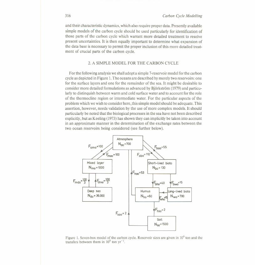
For the following analysis we shall adopt a simple 7-reservoir model for the carboncycle as depicted in Figure 1.The oceans are described by merely two reservoirs: onefor the surface layers and one for the remainder of the sea. It might be desirable toconsider more detailed formulations as advanced by Bjorkstrom (1979) and particu-larly to distinquish between warm and cold surface water and to account for the roleof the thermocline region or intermediate water. For the particular aspects of theproblem which we wish to consider here, this simple model should be adequate. Thisassertion, however, needs validation by the use of more complex models. It shouldparticularly be noted that the biological processes in the sea have not been describedexplicitly, but as Keeling (1973) has shown they can implicitly be taken into accountin an approximate manner in the determination of the exchange rates between thetwo ocean reservoirs being considered (see further below).

Atmosphere

Noo=700

Mixed loyer

Nmo=1000

Short-lived bioto

Nbo= 130

Fhoo=53

F. -100mdo-T Ed=100

me 3Fbho=40 Fbwo=15

Deep seo

Ndo= 36.000

Humus

Nho =60

Long-lived bioto

Nwo=7oo

Fsoo=2Fhso=2

Soil

Nso=1500

Figure 1. Seven-box model of the carbon cycle. Reservoir sizes are given in 109 ton and thetransfers between them in 109 ton yr -1.

Steady state and response characteristics 317

The terrestrial biota are described in terms of merely one ecosystem with fourmajor components: (b) shortlived biota active in assimilation and growth (leaves,needles, fine roots etc); (w) long-livedbiota which form the livingstructures (wood,bark, branches, etc); (h) dead organic matter which decomposes rapidly,humus; (s)dead organic matter in the soil, which decomposes slowly.

The magnitudes ofthe different reservoirsdefined in this wayand the present ratesof exchange between them (see Figure 1)have been based primarilyon the analysisby Whittaker and Likens (1975),Schlesinger(1977),and Bolinet at.(1979).Severalofthe estimates are quite uncertain and in a few instances alternate values have beenused to test the sensitivityofthe results to such changes. A more thorough treatmentusing a more detailed model is desirable.

All exchange processes within the ocean and the terrestrial biosphere will bedescribed as first order exchange processes, while the exchange between the atmo-sphere and the sea and the atmosphere and the terrestrialbiota willbe defined morecarefully,essentiallyfollowingthe treatment by Keeling (1973).In the case of the air-sea exchange the buffering of sea water willbe included. The photosynthesis oftheterrestrial biota will be dependant on both the atmospheric CO2concentration andthe amount of photosynthesizing matter which introduces a non-linearity into thesystem.

We shall use the following notations.Nj is the amount of carbon in reservoir i, where

1 = a denotes the atmospherem mixed layer of the oceand deep seab short-lived biotaw long-lived biotah humuss soil

Pmdenotes the partial pressure of CO2 in the mixed layerFij is the annual flux from reservoir i to j

Furthermore,

Nj = Njo + nj (2.1)

where Njo is the steady state amount in reservoir (i) and nj is the departure from

steady state conditions. Similarly Fijo denotes the steady state flux.kij is the first order exchange coefficient.

Fijo

kij = Njo(2.2)

*Nj, *Nio,*nj correspondingly, denote the amounts of radiocarbon in reservoir (i)


*Nj = *Nio+ *nj (2.3)

*Nj *nR--.k--

j - N. ' j - N .1 1

(2.4)

A is the radioactive decay constant for radiocarbon.

aij is the 14Cfractionation for transfer from reservoir (i) to G).Vi is volume of the ocean reservoirs, i = m, d.Yiis the annual input or removal of carbon to or from reservoir i caused by man'sactivities.

*Yais the annual formation of radiocarbon in the atmosphere due to cosmic radiation

The air-sea exchange requires special consideration. Following Keeling (1973) wehave

Fam = kam (Nao + na)Nao

Fma = kam (Nao + f-=- nm)Nmo

(2.5)

We shall not consider the gravitationalflux from the mixed layer to the deep seaexplicitly,but rather we shallfollowthe approach givenby Keeling (1973).The coef-ficients, kmdand kdm, are related by

- Ndo . kdmkmd -N mo

(2.6)

and in the equations for 14Ctransfer a fractionation coefficient adm is introduced

Nmo- +-

adm - amg VmVd (1-amg)Ndo

(2.7)

where amg is the fractionation of 14Cduring photosynthesis. Since amg is close tounity, the same is true for adm and no appreciable error is introduced in assumingadm = 1.

For the photosynthesis and respiration we assume the following relations

Na ,8 Nb ,8Fab = Fabo (- ra (- rb

Nao Nbo

NbFba = Fbao-

Nbo

which by linearization (nb <%;Nbo) can be transformed into

(2.8)

na nbFab = Fabo (1 + fia - + fib - )

Nao Nbo(2.9)


nbFba = Fbao (1 + -)

Nbo

In steady state we have, as depicted in Figure 1.

- Fomo-Fobo+Fmoo +Fboo +Fhoo +Fsoo=0

+Fomo -Fmoo-Fmdo+Fdmo =0

+Fmdo-Fdmo =0

-Fboo-Fbwo-Fbho =0

+Fbwo -Fwho =0

+Fbho+ Fwho-Fhoo -Fhso =0

+Fhso -Fsoo =0

+Fobo

(2.10)

For the time dependant case we get the following set of equations

d F. bo Noo II 'boo Fooo)(-+k +Q ..Q )n -k 1;:-n +(I'b-- - nbdt om 1'0Noo a am ~ Nmo m Nbo Nbo

( d Noo )-komno+ dT+kom~ N +kmd nm-kdmndmo

-kmd nm+ (ddt +kdm)nd

_~oFObOno +(ddt -~b~+~+kbh+kbW)nbNoo bo bo

-kho nh-ksons =Yo

=Ym

=Yd

=Yb

-kbw nb+(it+ kwh)nw

-kbh nb-kwhnw+ (ddt +kho+khs) nh

=Yw

=Yh

-khsnh+(gt +kso)ns = Ys

(2.11)


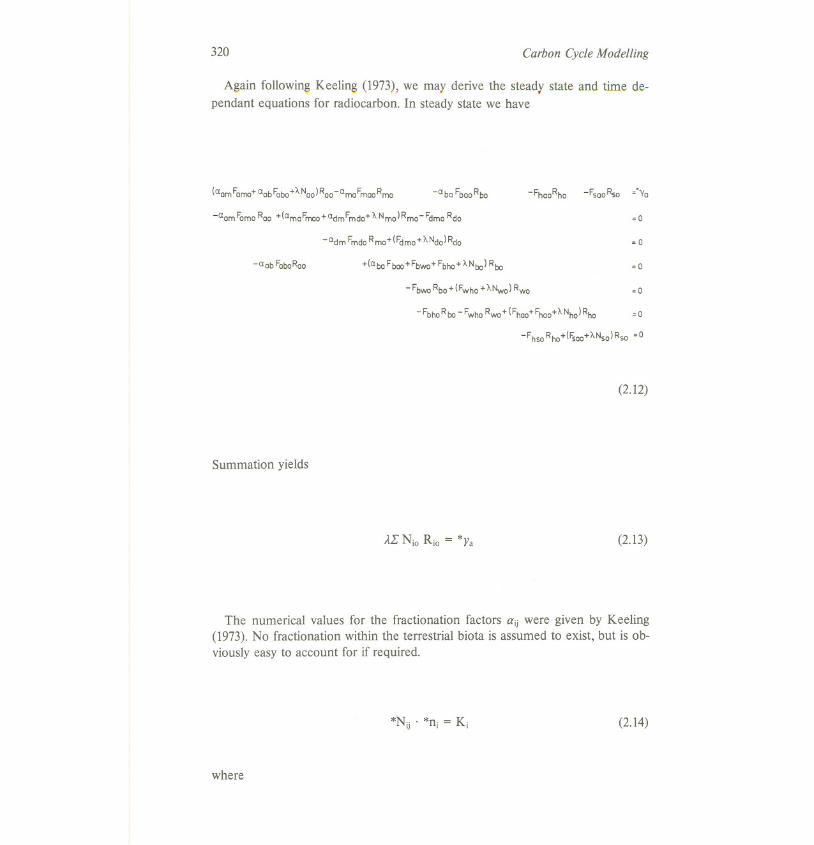
Again following Keeling (1973), we may derive the steady state and time de-pendant equations for radiocarbon. In steady state we have

(ClamFamo+ ClabFaba+ANaa)Raa -ClmaF maaRma -Clba FbaoRbo -FhaaRha -FsaoRso ;.Ya

-ClamFamoRoo +(ClmaFmoo+CldmFmda+ANma)Rma-Fdma Rdo ;0

-Cldm Fmdo Rmo+(Fdmo+ANdo) Rdo ;0

-Clab FaboRaa +(Clba Fboo+Fbwa+ Fbho+ ANbo) Rbo ;0

-FbwoRbo+(Fwho +ANwo) Rwo ;0

-FbhoRbo - Fwha Rwa + (Fhao+ Fhao+A Nho) Rho ;0

-FhsoRho+(Fsao+ANso)Rsa ;0

(2.12)

Summation yields

,.11' Nio Rio = *Ya (2.13)

The numerical values for the fractionation factors aij were given by Keeling(1973).No fractionation within the terrestrial biota is assumed to exist, but is ob-viously easy to account for if required.

*Nij . *nj = Kj (2.14)

where


""""',< V)+ ......

00 N

U'IU'I '-'

.:.: 0 0 0 0 0 .:.:I +

-01;::;,<+ U'IU'I

0 ..c::; ..c::;.:.: .:.:

..c::;0 0 0 0 + I.:.:

I 0..c::;

.:.:+

-01;::;

',<+..c::; ..c::;

0 0 0 0 0.:.: .:.:+ I

.8-01;::;

,<u:Z +

I ..c::;.c

J}.:.:+

..c::;.c .c .c .cC!2.-0

.:.: .:.: .:.:.c

0 0..:!:. I I 0

1::1

01 0I 0 .c

iEzI

.81 0IE.c

C!2.-0.ctj+

-01;::;,<

E +E0 -0 .:.:-0 0 0 0 0.:.:

I +

,< -01;::;

0 +

.pJ ;IJE E0 -0

.:.: .:.:0 EE -0 01:1

1::1 01 EI

oj.pz -0 0W).:.: 0 0 0

E E.:.:0 J'0 I

E1::1+

,<-01;::;

+

JlE .81 0.c 0 IE-P

0 .:.: d'.1::1+ E 0 .c 0 0 0E 0

1::100 1::1.:.: I I

E0

1::1+

-01;::;-ii,='Z*

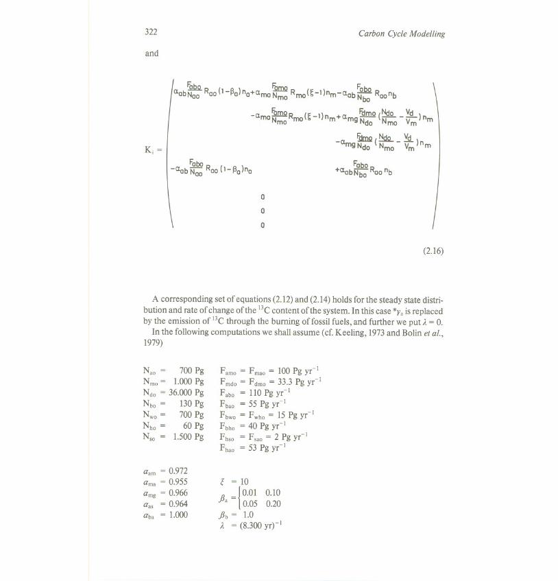
322

and

Carbon Cycle Modelling

~ '11m2 - - Foboa.obNooRoo(1-~0) no+a.moNmoRmo(~ 1)nm <labNbo Roonb

Fomo( )

Fdmo( Ndo Vd

)-a.mo-N Rmo ~-1 nm+a.mg-N N -y- nmmo do mo m

~-~ 1\1-,- Vd-a. ~ (:..:yjL- -)n

mgNdo Nmo Vm mK -j-

Fobo-<lab Noo Roo (1-130)no

Fobo+<lobNbo Roonb

0

0

0

(2.16)

A corresponding set of equations (2.12) and (2.14) holds for the steady state distri-

bution and rate of change of the l3e content of the system. In this case *Yais replacedby the emission of l3e through the burning of fossil fuels, and further we put A = O.

In the following computations we shall assume (cf. Keeling, 1973 and Bolin et al.,1979)

Nao = 700 PgNmo = 1.000 PgNdo = 36.000 PgNbo = 130 PgNwo = 700 PgN ho = 60 PgNso = 1.500 Pg

aam = 0.972ama = 0.955

amg = 0.966aas = 0.964aba = 1.000

Famo = Fmao = 100 Pg yr-lFmdo = Fdmo = 33.3 Pg yr-lFabo = 110 Pg yr-lFbao = 55 Pg yr-lFbwo = Fwho = 15 Pg yr-lFbho = 40 Pg yr-lFhso = Fsao = 2 Pg yr-lFbao = 53 Pg yr-l

<; = 10

fi ={

0.01 0.10a 0.05 0.20

fib = 1.0A = (8.300yr)-l


3. STEADY STATES,PRESENT AND PAST

The systems of equations (2.10) and (2.12) defme the steady state distribution of12Cand 14Cbetween the seven reservoirs, in the latter case in response to a constantrate of 14Cproduction, *Ya.The former system, (2.10), essentially only implies a con-sistency in the estimates from observations of the fluxes between the reservoirs. Theexceptions are the air sea exchange and the exchange within the oceans where the14C-distribution has been utilized as well (Craig, 1957; see further below). With theaid of (2.2) and the estimates of the reservoir sizes we also obtain a value for theexchange coefficients, kij, required for the maintenance of a steady state. The estim-ate of Fdmoand thus ofkdm is based on the value ofRdo, the third equation (2.12) andthe assumption that F mdo= F dmo.A deviation of real conditions from a steady statemay imply a considerable error in the estimate of kdm. 14Cobservations from thedeep sea (Rd) are available for merely about 20 years, which is much too short a timeto reveal possible deviations from a steady state.

Most simulations of future changes of the carbon cycle have been based on anassumption that an approximate steady state prevailed at the beginning of the in-dustrial revolution in the middle of the last century and the determination of some

features of the cycle by asking for the best possible fit between the model and realityduring the rather short period for which data are available. The assumption of aninitial steady state is crucial for this approach. Because we do not know how accuratethis approximation is, a considerable degree of uncertainty is introduced that hasusually not been taken into account We shall later explicitly investigate the implica-tions, if this assumption is not valid. In the remainder of this section some other pos-sible steady states will be discussed.

Comparisons between radiocarbon age and real age of tree rings show consider-able differences (Suess, 1970) with variations on time scales of a few hundred years.The radiocarbon age also becomes increasingly less than the real age when goingback 4.000 to 6.000 years in time. The maximum difference is about 900 years andhas been explained as a result of a more intense magnetic field, whereby the produc-tion of 14C by cosmic rays, *Ya,may have been greater. This explanation seemsplausible, since there is independant evidence that such changes may have occurredin the past (Bucha, 1970).

It is, however, interesting to note that measurements of the decrease of the 14Cwith depth in the bottom sediments, even if accounting for this possible change of*Ya,show a decrease of the sedimentation rate from 10.000 B.P. until present times(Peng et al., 1977). The rate of primary production in the sea therefore probably wasless during this time period. Since the primary production is dependant on the avail-ability of nutrients in the photic zone and since these are supplied by up-welling onemay ask if possibly the turn-over rate of the oceans may have been different at thattime. In this context it should be recalled that Worthington (1968) has advanced the

idea that the deglaciation about 10.000 years ago may have decreased the salinity ofthe polar waters to such an extent that the deep water formation may have been con-


siderably reduced or even completely inhibited. This reduction would then, how-

ever, also have changed the distribution of radiocarbon. Obviously a decrease of thedeep water formation would imply less radiocarbon in the deep sea, but also largeramounts in the other major reservoirs if the production rate, *y., remained the same.Let us assume that at anyone time an approximate steady state prevailed and deter-mine the 14Cin the various reservoirs for different values ofkdmo = F dmo/Ndo,for thepresent value of *Ya.

It was shown by Keeling (1973) that the present simple formulation of the carbonexchange in the oceans without considering the biological activity explicitly is a rea-sonable approximation if a steady state prevails. We use the reservoir sizes andexchange rates as given in Figure 1, but vary kdmo.The fractionation factors given byKeeling (1973) have been used. Figure 2 shows how the radiocarbon concentrationof the atmosphere and the two ocean reservoirs depend on kdmo.We denote the newvalues with Rio and Figure 2 shows R~o/Rao, R:no/Rao and Rcto/Rao, where Rao,denote the values for kdm-I = 1.000 years. Since no changes of the behaviour of theterrestrial biosphere have been assumed to occur, Rho/Rao, R~o/Rao, Rho/Rao andR~o/Rao change directly in proportion to R~o/Rao.

We note that R~oand R:no change considerably more than Rctodepending on themuch larger deep ocean water reservoir. R~o (and R:no) increase by 10% if kd~increases to about twice the present value, i.e. to about 2.000 years. This changewould be sufficient to explain the discrepancy of 900 years between radiocarbon ageand true age which has been observed for tree rings grown 6.000 years ago, without

600 500 1.00 k-~d years

100~m Pg y(l

Urn

kdrn -+ 00R'mo/Rdo/R~o

Rdo7RoO

Figure 2. Rio (i = a, m, d) as function of the rate of exchange between the deep sea and themixed layer, Fdm, or the turn-over time, Tdm= kd~.

1.151Rio1.10

1.05

1.001

10

0.95

Q90

0.85

0.80


any change of the radio-carbon production by cosmic radiation. It is interesting tonote that the sedimentation for the period 10.000-6.000B.P. that has been computedby Peng et al. (1977)are about 40%of the present rate. This value is in reasonableagreement with the notion that the rate of up-welling,nutrient supply to the photiczone and primary production is proportional to kdmoand thus 50%of the presentvalue (if kd~ = 2.000years). It should be remarked, however, that Peng et al. (1977)seems not to have corrected their estimates of sedimentation rates by consideringalso the difference between radiocarbon age and true age.

The computations summarized above are approximate and the data used are quitelimited. We therefore cannot conclude that the ocean circulation has varied duringpostglacialtime, even though the data referred to support such a conclusion. In viewof its important implications for the determination of past changes of climate theproblem warrants further attention.

4. TRANSIENT CHANGES IN THE CARBON CYCLE

The two sets of equations (2.11)and (2.14)describe the transient behaviour of thecarbon cycle due to external factors that influence the exchange of 12Cand therebyindirectly also the distribution of 14C.We shall in turn consider

1) The eigencharacteristics of the systems2) The adjustment in time of an initial departure from equilibrium3) The response of the carbon cycleto an exponentiallyincreasingsource term Yafor

different rates of increase

4) The response of the carbon cycleto a periodic variation of the surface water tem-perature

4.1 THE EIGENCHARACTERISTICS OF THE CARBON CYCLE

The eigenfrequencies of the system (2.9) with the values ofFijo and Nio (and thuskij) as given in section 2 are (fla = 0.10)

VI = -1.17 yr-I TI = 0.85 yrV2= -0.91 yr-l T2 = 1.09 yrV34 = -0.0210 :t i 0.042 yr-I T3 4 = 48 :t i 150 yrV4'= -0,0034 yr-I Ts' = 300 yrV6= -0.00092 yr-I T6 = 1090 yrV7= 0 T7 = 00

The range of Viis the same as for kij.We note further that there is one pair of complexeigenfrequencies permitting damped oscillations (see 4,2), This appears because ofthe time delay of transfer through the terrestrial biota. Other values.fJa (0,01 ;;;afta;;;a

0.20) donotgreatlyinfluencetheprinciplefeaturesasrevealedbythe eigenfrequen-cies given forfta = 0.10. It should be emphasized, however, that the nonlinear equa-tions that describe finite changes in the system have been linearized, whereby a more


complex behaviour of the system has been possiblyeliminated. For a more detailedanalysis of such a possibility reference is made to an early paper by Eriksson andWelander (1956).

4.2 THE ADJUSTMENT OFAN INITIAL DEPARTURE FROM EQUILIBRIUM

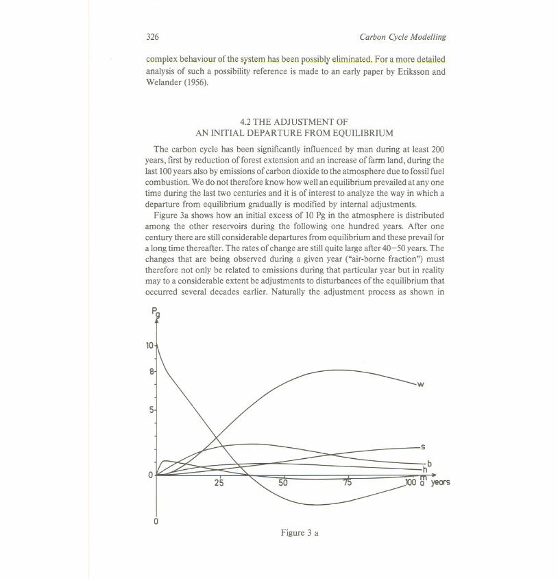
The carbon cycle has been significantlyinfluenced by man during at least 200years, first by reduction of forest extension and an increase of farm land, during thelast 100years alsoby emissionsof carbon dioxide to the atmosphere due to fossilfuelcombustion. We do not therefore know how wellan equilibriumprevailedat anyonetime during the last two centuries and it is of interest to analyze the way in which adeparture from equilibrium gradually is modified by internal adjustments.

Figure 3a shows how an initial excess of 10 Pg in the atmosphere is distributedamong the other reservoirs during the following one hundred years. After onecentury there are stillconsiderable departures from equilibrium and these prevail fora long time thereafter. The rates of change are stillquite largeafter 40- 50years.Thechanges that are being observed during a given year ("air-borne fraction") musttherefore not only be related to emissions during that particular year but in realitymay to a considerable extent be adjustments to disturbances of the equilibrium thatoccurred several decades earlier. Naturally the adjustment process as shown in

8w

10

5

s

25hb

~O H' years0

0Figure 3 a


10

75 y<!OI"S

Pg10

25 50 75

bm

100Veors-

Pg

25 50 100 Yeors

-5

/-10

Figure 3. The adjustments of various reservoirs followinga disturbance ofa) the addition of 10 Pg to the atmosphere, fi = 0.10.b) the addition of 10Pg to the atmosphere and withdrawal of 10 Pg from long-lived biota,

i.e. wood, fl = 0.10.c) the same as a) butfi = 0.01.d) the same as b) butfi = 0.01.


Figure 3a is criticallydependant on the parameters chosen to describe the carboncycle.The markedincreaseof nwis a responseto the increaseof nb,which in turndepends on the value chosen forfia. A smaller value forfia delays the decrease of navery considerably,whereby nmalso remains positivelonger permitting a build up ofnct(see Figure 3c). Most of the excess carbon injected into the atmosphere in anycase ultimately ends up in the deep sea, but for a small value offia much less passesvia the terrestrial biota as illustrated in Figure 3a.

Another example is shown in Figure 3b in which the initialdisturbances are nao=10Pg and nwo= -10 Pg, i.e. no net change of the total amount of carbon in the sys-

tem isintroduced. Such a situationwould result from the burning offorests. We notethat adjustments back to a steady state are quicker than in the previous example,because the reservoirs with slow response, i.e. the deep sea and the soil, never getmuch involvedin this case. Again a smallvalue forfia delaysthe changes as shown inFigure 3d. However in simulatingthe expansion of agriculture byputting nao= 10Pgand nso = -10 Pg, we find much more long lasting effects on the carbon cyclebecause of the slow turn-over time for carbon in soils.

4.3 THE RESPONSE TO AN EXPONENTIALLYINCREASINGSOURCETERMYa.

The emission of carbon dioxide to the atmosphere by fossil fuel combustionduring the last 100 years can be approximated reasonably well by an exponentialfunction V= Voexp (at), where a = 0.03years-I. (The increase wassignificantlylowerduring the two worldwars and alsoduring the economic depression in the beginningof the 1930's.)The response of the carbon cycle to such an increase may be con-sidered as the sum of a forced exponential solution to equations (2.11) and adjust-ments (solutions to the homogenous equations (2.11», which tend towards zero astime becomes large compared with the periods defined by the eigenfrequencies ofthe system. The character of the adjustments is determined by the initialconditions,and thus depends also on whether the system initiallyis in equilibrium or not. For adetailed comparison between the model and reality the complete solution of coursemust be considered, which, however, is uncertain if initial conditions are not wellknown. It is of interest to have a look at merely the forced solution since it wellreveals the general behaviour of the system, particularly its dependance on the ratewith which the external influence is imposed on the system.

With Ya= Vaoexp (at) the forced (particular)solution of equations (2.11)isgiven by

nj = nio exp (at)l"nio = Vaola (4.1)

Table 1 shows n;o, i = a, m, . . . s in percent of Yaola for values of a = 0.5, 1,2 . . . 8%

We note that the partitioning between the various reservoirs very much dependson the rate of increase, a. For small values of a the uptake by the oceans is small,while the more accessible reservoirs of terrestrial biota and soil are the importantsinks. The result is, however, sensitive to the choice of fia and fib as is shown byKohlmaier (chapter 5, this volume). Particularly for valuesfib > 1 the biota quicklydecreases in importance as a sink (cf the behaviour of the solutions presented byRevelle and Munk, 1977).

4.4 THE RESPONSE OF THE CARBON CYCLE TO A PERIODICVARIATION OF THE SURFACE WATER TEMPERATURE

Bacastow (1978) and MacIntyre (1978) have analyzed to what extent temperaturechanges of the surface water may cause variations of the carbon dioxide concentra-tions in the atmosphere. MacIntyre points out the importance of considering thebuffering characteristics of sea water for properly evaluating the effect of a tempera-ture change on the equilibrium partial pressure. Let P denote the partial pressure, Tthe temperature, and C the concentration of total inorganic carbon in sea water,while I: denotes the total amount of carbon in the gas phase and in solution.MacIntyre (1978) emphasizes that (6PI6T)c "'" 16-18 ppm/oC is very much largerthan (6P16Th = 1.3-1.5 ppm/oC and that the temperature effect in reality is there-fore much reduced. Bacastow (1978) analyzes the implications of this in a simplemodel of the carbon cycle and shows that the carbon dioxide variations observed inassociation with the Southern Oscillation could be explained by a temperature varia-tion of about :tl°C.

It is of interest in the present context to analyze the effect of temperature varia-tions of different frequencies for the somewhat more general carbon cycle used here.Following Bacastow (1978) we have

Steady state and responsecharacteristics 329

Table 1.niol (Yaola) in percent for i =a, m, d ...s, for different rates of the emissionincrease, a.

nia a%

Yaala 0.5 1.0 2.0 3.0 4.0 6.0 8.0

i = a 3.7 8.7 19.5 29.5 38.0 50.6 59.0m 0.5 1.2 2.7 4.0 5.1 6.6 7.6

d 2.8 3.6 4.2 4.3 4.1 3.6 3.1b 11.5 13.7 15.4 15.5 14.9 13.3 11.6h 5.0 5.7 6.0 5.8 5.4 4.6 3.9w 50.0 50.3 42.8 34.8 28.0 18.8 13.2s 26.4 16.8 9.4 6.2 4.4 2.5 1.6


6Pm 6PmoPm = (- )T oCm + (-)c oT6Cm 6T m

where index ( )mas before denotes the mixed layerand 6 indicates smalldeviationsfrom equilibrium. From Keeling (1973)and Bacastow (1978)we get

(4.2)

6Pm 6Nm 1 6Pm6Fma = kamNao - = kamNao ~- + - (-)C 6TPm Nmo Pm 6T m

The first term has been included in (2.11)(6Nm=nmfor small nm),and we canaccount for the influence of a varying temperature on the changes of nj by putting

(4.3)

1 6PmYa = kamNao - (-)C 6T = - YmPm 6T m

Assuming Pm-1 ( 6PmI6T)Cm = 0.04

Ya= 4 . 6T = - Ym

(4.4)

we obtain

(4.5)

We insert the expression (4.4)with the numerical value given in (4.5)into (2.11)andassume a periodic variation of 6T with different frequencies. The amplitude of theassociated periodic variations of na are shown in Figure 4.

ppm

1.0

2.0

010 20 30 40 years

Figure 4. The amplitude of the variations of the atmospheric concentration (parts permillion) of carbon (in the form of carbon dioxide) due to a periodic change of the tempera-ture ofthe mixed layerwith an amplitude of loe and as dependant on the period of the forcing.


For a period T = 4 years, which corresponds to the period of the Southern Oscilla-

tion, the result agrees well with that of Bacastow (1978). Since the response dependsprimarily on the rate of exchange between the atmosphere and the mixed layer of the

sea, which is rapid, an approximate equilibrium between these two reservoirs pre-

vails at anyone time for variations with a period of 5-10 years and longer. No further

appreciable increase of the amplitude of na occurs for larger values of T.For quick

temperature changes, however, there is not enough time to have a quasi-equilibriumestablished; the amplitude of na is correspondingly less and the phase lags behind

that of aT. For annual variations it is merely 0.4 ppm. In reality, therefore, little of the

annual variations of na are probably caused by the annual variations of ocean

temperature.

REFERENCES

Bacastow,R.B. (1978)Dip in the atmospheric CO2level during the mid 1960's.J. Geoph. Res.Bjorkstrom, A. (1979) A model of the CO2 interaction between atmosphere, oceans and

land biota. In Bolin, B., Degens, E.T., Kempe, S., Ketner, P. (eds), The global carboncycle, SCOPE Report, 13,403-457, J. Wiley & Sons, Chichester.

Bolin, B., Degens, E.T., Duvigneaud, P. and Kempe, S. (1979)The global biogeochemicalcycle of carbon. In Bolin, B., Degens, E.T., Kempe, S., Ketner, P. (eds), The globalcarbon cycle, SCOPE Report, 13, I-56, J. Wiley & Sons, Chichester.

Bucha, V. (1970) Evidence for changes in the Earth's magnetic field intensity. Phil.Trans. Roy. Soc. A 269.47-55.

Craig, H. (1957)The natural distribution of radiocarbon and the exchange time of carbondioxide between atmospere and sea. Tellus, 9, 1-17.

Eriksson, E. (1963) Possible fluctuations in atmospheric CO2 due to changes in the pro-perties of the sea. J. Geoph. Res., 68, 3871-3876.

Eriksson, E. and Welander, P. (1956) On a mathematical model of the carbon cycle innature. Tellus, 8. 155-175.

Keeling, C.D. (1973) The carbon dioxide cycle: Reservoir models to depict the exchangeof atmospheric carbon dioxide with the oceans and land plants. In: Rasool, S.I. (ed),Chemistry of the lower atmosphere, 251- 329, Plenum Press, New York.

Macintyre, F. (1978)On the temperature coefficient of PC02in sea water. Climatic change,1, 349-354.

Peng, T.-H., Broecker, W.S., Kipphut, G. and Shackleton, N. (1977) Benthic mixing indeep sea cores as determined by 14Cdating and its implications regarding climate strati-graphy and the fate of fossil fuel CO2. In: Andersson, N., Malahoff, A. (eds) The fateof fossil fuel CO2 in the oceans, 355- 373.Plenum Press, New York.

Revelle, R., Munk, W. (1977)The carbon dioxide cycle and the biosphere. In: Energy andclimate. Stud. Geophys. 140-158. Nat Acad. of Sciences, Washington, D.C.

Schlesinger, W.H. (1977)Carbon balance in terrestrial detritus. Am. Rev. Ecol. Syst 51-81.Suess, H. (1970)The three causes of the secular C14 fluctuations and their time constants.

In: Olsson, I. (ed) Radiocarbon variations and absolute chronology, 595-605, Proc.Twelfth Nobel Symp. Almqvist & Wicksell, Uppsala.

Whittaker, R.H. and Likens, G.E. (1975)The biosphere and man. In "Primary productivityof the bIosphere". Ecological Studies, 14, 305- 32S,Springer Verlag, B~rlin.

Worthington, L.V. (1968) Genesis and evolution of water masses, Meteorological mono-graphs, Am. Met Soc. Boston, Mass., Vol. 8,63-67.

Documents

Steady State and Response Characteristics of a … State and Response Characteristics of a Simple Model of the Carbon Cycle BERT BOLIN ABSTRACT A model of the carbon cycle with seven