Embed Size (px)
DESCRIPTION
Stay or Go? A Q-Time Perspective. H. John B. Birks University of Bergen, University College London & University of Oxford. Stay or Go – Selbusjøen February 2011. What is Q-Time?. - PowerPoint PPT Presentation
Citation preview
Stay or Go?A Q-Time Perspective
H. John B. Birks
University of Bergen, University College London & University of Oxford
Stay or Go – Selbusjøen February 2011
What is Q-Time?
Most ecologists interested in time-scales of days, weeks, months, years, decades, or even centuries – Real-time or Ecological-time
Palaeobiologists and palaeoecologists interested in time-scales of hundreds, thousands, and millions of years.
• Deep-time – pre-Quaternary sediments and fossil record to study evolution and dynamics of past biota over a range of time-scales, typically >106 years.
• Q-time or Quaternary-time – uses tools of paleobiology (fossils, sediments) to study ecological responses to environmental changes at Quaternary time-scales (103-105 years) during the past 2.6 million years. Concentrates on last 50,000 years, the window dateable by radiocarbon-dating. Also called Near-time (last 1-2 million years).

Do Q-Palaeoecology and Stay or Go Belong Together?
Quaternary palaeoecology traditionally concerned with reconstruction of past biota, populations, communities, landscapes (including age), environment (including climate), and ecosystems
Emphasis on reconstruction, chronology, and correlation
Been extremely successful but all our hard-earned palaeoecological data remain a largely untapped source of information about how plants and animals have responded in the past to rapid environmental change
“Coaxing history to conduct experiments” E.S. Deevey (1969)
Brilliant idea but rarely attempted. Recently brought into focus by the Flessa and Jackson (2005) report to the National Research Council of the National Academies (USA) on The Geological Record of Ecological Dynamics

Important and critical role for palaeoecology. The Geological Record of Ecological Dynamics – Understanding the Biotic Effects of Future Environmental Change (Flessa & Jackson 2005)
Three major research priorities
1. Use the geological (= palaeoecological) record as a natural laboratory to explore biotic responses under a range of past conditions, thereby understanding the basic principles of biological organisation and behaviour: The geological record as an ecological laboratory ‘Coaxing history to conduct experiments’.
2. Use the geological record to improve our ability to predict the responses of biological systems to future environmental change: Ecological responses to environmental change
3. Use the more recent geological record (e.g. mid and late Holocene and the ‘Anthropocene’) to evaluate the effects of anthropogenic and non-anthropogenic factors on the variability and behaviour of biotic systems: Ecological legacies of societal activities
.
Palaeoecology can also be long-term ecology
Basic essential needs in using the palaeoecological record as an ecological laboratory for Stay or Go
1. Detailed biostratigraphic data of organism group of interest (e.g. plants – pollen and plant macrofossil data). Biotic response variables
2. Independent palaeoenvironmental reconstruction (e.g. July air temperature based on chironomids). Predictor variable or forcing function
3. Detailed fine-resolution chronology
Can look at Stay or Go in a long-term Q-time perspective
Why is a Q-Time Perspective Relevant?
Long argued that to conserve biological diversity, essential to build an understanding of ecological processes into conservation planning
Understanding ecological and evolutionary processes is particularly important for identifying factors that might provide resilience in the face of rapid climate change
Problem is that many ecological and evolutionary processes occur on timescales that exceed even long-term observational ecological data-sets (~100 yrs)
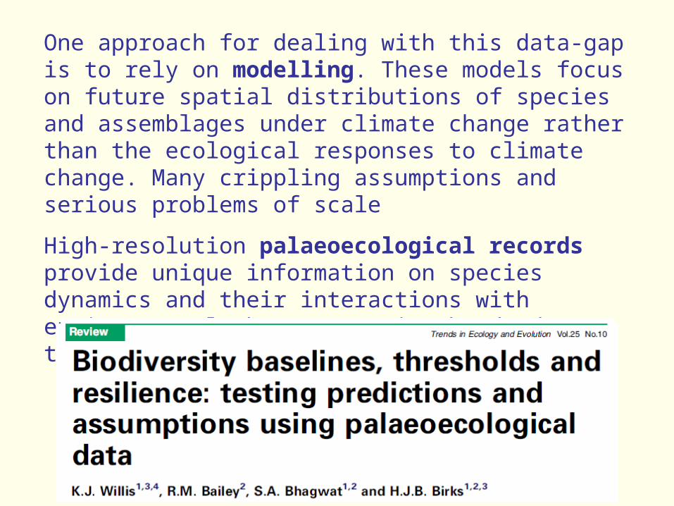
One approach for dealing with this data-gap is to rely on modelling. These models focus on future spatial distributions of species and assemblages under climate change rather than the ecological responses to climate change. Many crippling assumptions and serious problems of scale
High-resolution palaeoecological records provide unique information on species dynamics and their interactions with environmental change spanning hundreds or thousands of years

How did Biota Respond to a Past Rapid Climate Change?
The end of the Younger Dryas at 11700 years ago is a perfect ‘natural experiment’ for studying biotic responses to rapid climate change
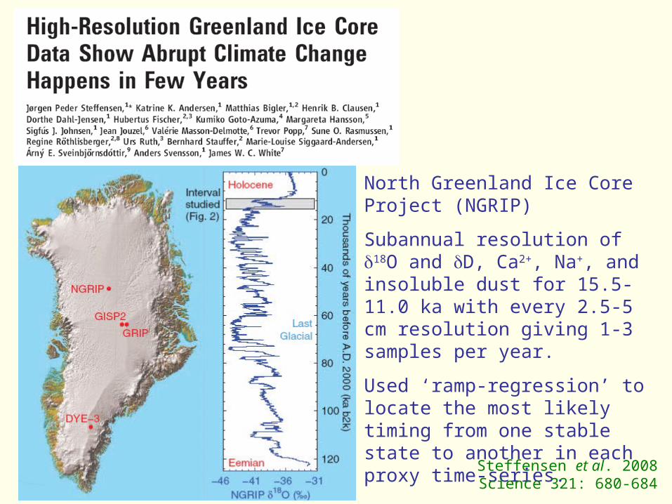
North Greenland Ice Core Project (NGRIP)
Subannual resolution of 18O and D, Ca2+, Na+, and insoluble dust for 15.5-11.0 ka with every 2.5-5 cm resolution giving 1-3 samples per year.
Used ‘ramp-regression’ to locate the most likely timing from one stable state to another in each proxy time-series.
Steffensen et al. 2008 Science 321: 680-684

YD-Holocene at 11.7 ka
deuterium excess (d) ‰
18O ‰
log dust
log Ca2+
log Na+
layer thickness ()
Annual resolution
Ramps shown as barsSteffensen et al. 2008
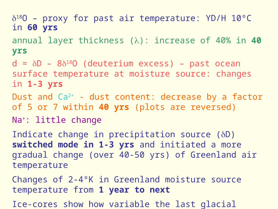
18O – proxy for past air temperature: YD/H 10ºC in 60 yrs
annual layer thickness (): increase of 40% in 40 yrs
d = D – 818O (deuterium excess) – past ocean surface temperature at moisture source: changes in 1-3 yrs
Dust and Ca2+ - dust content: decrease by a factor of 5 or 7 within 40 yrs (plots are reversed)
Na+: little change
Indicate change in precipitation source (D) switched mode in 1-3 yrs and initiated a more gradual change (over 40-50 yrs) of Greenland air temperature
Changes of 2-4ºK in Greenland moisture source temperature from 1 year to next
Ice-cores show how variable the last glacial period was – no simple Last Glacial Maximum

Kråkenes Lake, Western Norway
Birks et al. 2000


Palaeoecological data
1. Pollen analysis by Sylvia Peglar600-769.5 cm 117 samples101 taxa 16 aquatic taxa
2. Macrofossil analysis by Hilary BirksPollen analyses supplemented by plant macrofossil analyses that provide unambiguous evidence of local presence of taxa, for example, birch trees
3. Chironomid analysisPast temperatures estimated from fossil chironomid assemblages by Steve Brooks and John Birks
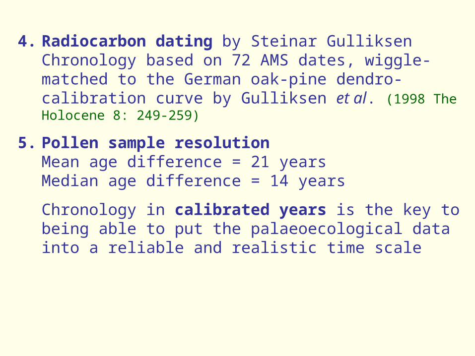
4. Radiocarbon dating by Steinar GulliksenChronology based on 72 AMS dates, wiggle-matched to the German oak-pine dendro-calibration curve by Gulliksen et al. (1998 The Holocene 8: 249-259)
5. Pollen sample resolutionMean age difference = 21 yearsMedian age difference = 14 years
Chronology in calibrated years is the key to being able to put the palaeoecological data into a reliable and realistic time scale

600
610
620
630
640
650
660
670
680
690
700
710
720
730
740
750
760
770
Dep
th (
cm)
9200
9400
9600
9800
10000
10200
1040010600
10800
11000
11200
11400
11600
Cal
ibra
ted
year
s B
P
20 40
Loss
-on-
ignitio
n at
550
o C
Saxifr
aga
oppo
sitifo
lia-ty
pe
Ranun
culus
glac
ialis-
type
20
Sedum
20
Capse
lla-ty
pe
20
Rumex
ace
tose
lla-ty
pe
Koenig
ia isl
andic
a
Oxy
ria d
igyna
20 40
Salix u
ndiff.
20
Salix h
erba
cea-
type
20
Gram
ineae
20
Carex
-type
20 40
Dryop
teris
-type
Filipen
dula
Rumex
ace
tosa
20
Empe
trum
nigr
um
20
Junip
erus
com
mun
is
20 40
Betula
Gymno
carp
ium d
ryop
teris
Polypo
dium
vulga
re a
gg.
Populu
s tre
mula
20
Pinus
sylve
stris
20
Corylu
s av
ellan
a
Sorbu
s cf
. S.a
ucup
aria
Zone
7
6
5
4
321
KrakenesEarly Holocene - Major Taxa
Percentages of Calculation Sum
Lith
olog
y
°
Two statistically significant pollen zone boundaries in 110 years since YD, 3 zone boundaries in 370 years, 4 zone boundaries in 575 years, and 5 zone boundaries in 720 years (first expansion of Betula).
Very rapid pollen stratigraphical changes and hence rapid vegetational dynamics. Birks & Birks 2008
YD
EH
665
670
675
680
685690
695
700
705
710
715
720
725
730735
740
745
750
755
760
765
770
Dep
th (c
m)
10,920
10,870
11,180
11,270
11,385
11,530
Cal
1
4 C y
r BP
20 40 20 20 20 500 1000 1500 20 40 1000 2000 50100 20 20 40 20 20 40 60
EH
YD
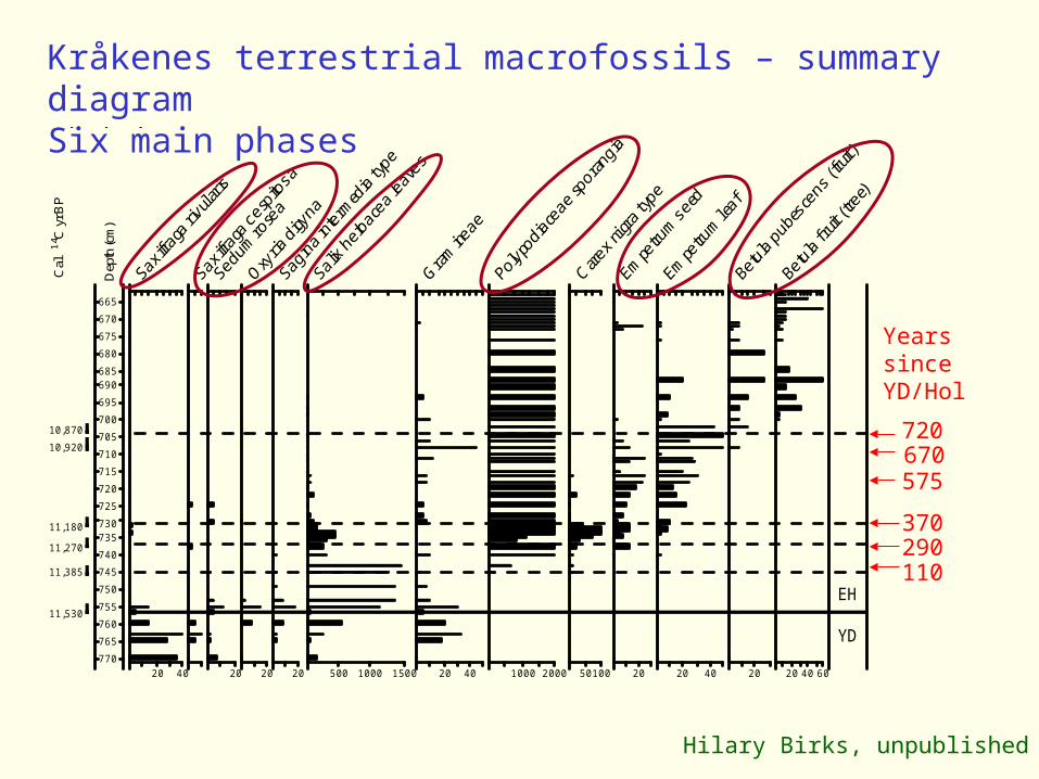
Kråkenes YD/HoloceneSelected plant macrofossil taxa
Analysed by Hilary H. Birks
Kråkenes terrestrial macrofossils – summary diagramSix main phases
Hilary Birks, unpublished
110290
720
370
Years since YD/Hol
575670

Terrestrial vegetation & landscape development
Zone Age (cal yr BP)
Years since YD
7
10830 720
Betula woodland with Juniperus, Populus, Sorbus aucuparia, and later Corylus. Abundant tall-ferns. Betula macrofossils start at 10880 BP
610975 575
Fern-rich Empetrum-Vaccinium heaths with Juniperus
511180 370
Empetrum-Vaccinium heaths with tall-ferns. Stable landscape
411440 110
Species-rich grassland with tall-ferns, tall-herbs, and sedges. Moderately stable
311500 50
Species-rich grassland with wet flushes and snow-beds
211550 0
Salix snow-beds, much melt-water and instability
1YD
Open unstable landscape with 'arctic-alpines' and 'pioneers', amorphous solifluction
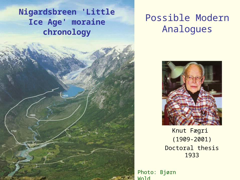
Nigardsbreen 'Little Ice Age' moraine
chronology
Photo: Bjørn Wold
Knut Fægri (1909-2001)
Doctoral thesis 1933
Possible Modern Analogues
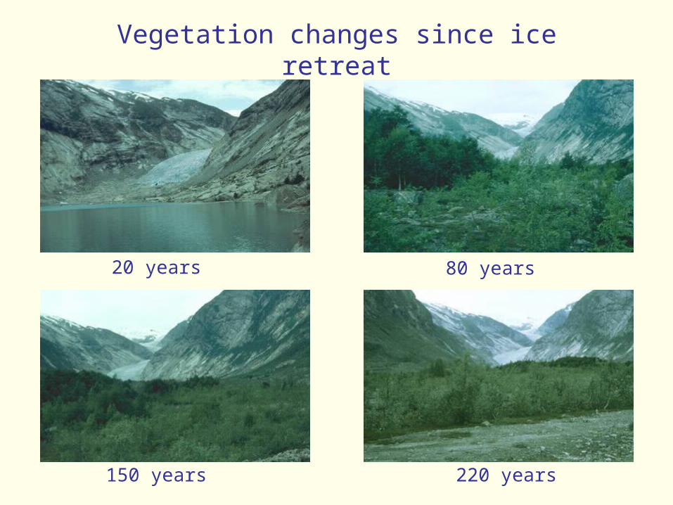
Vegetation changes since ice retreat
20 years 80 years
150 years 220 years
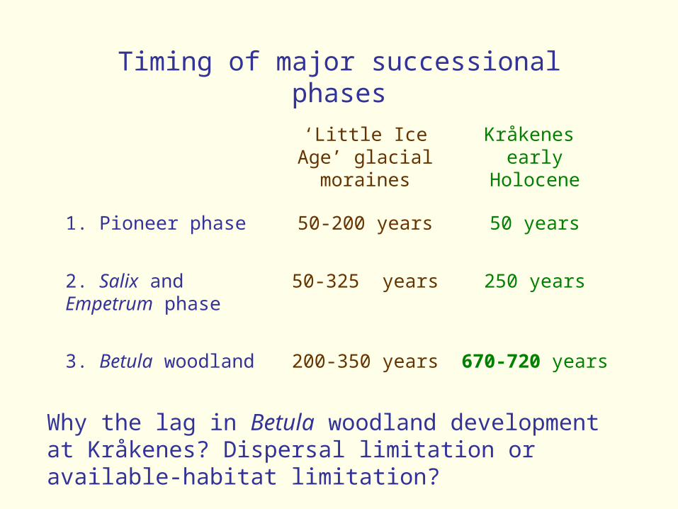
Timing of major successional phases
‘Little Ice Age’ glacial moraines
Kråkenes early Holocene
1. Pioneer phase 50-200 years 50 years
2. Salix and Empetrum phase
50-325 years 250 years
3. Betula woodland 200-350 years 670-720 years
Why the lag in Betula woodland development at Kråkenes? Dispersal limitation or available-habitat limitation?
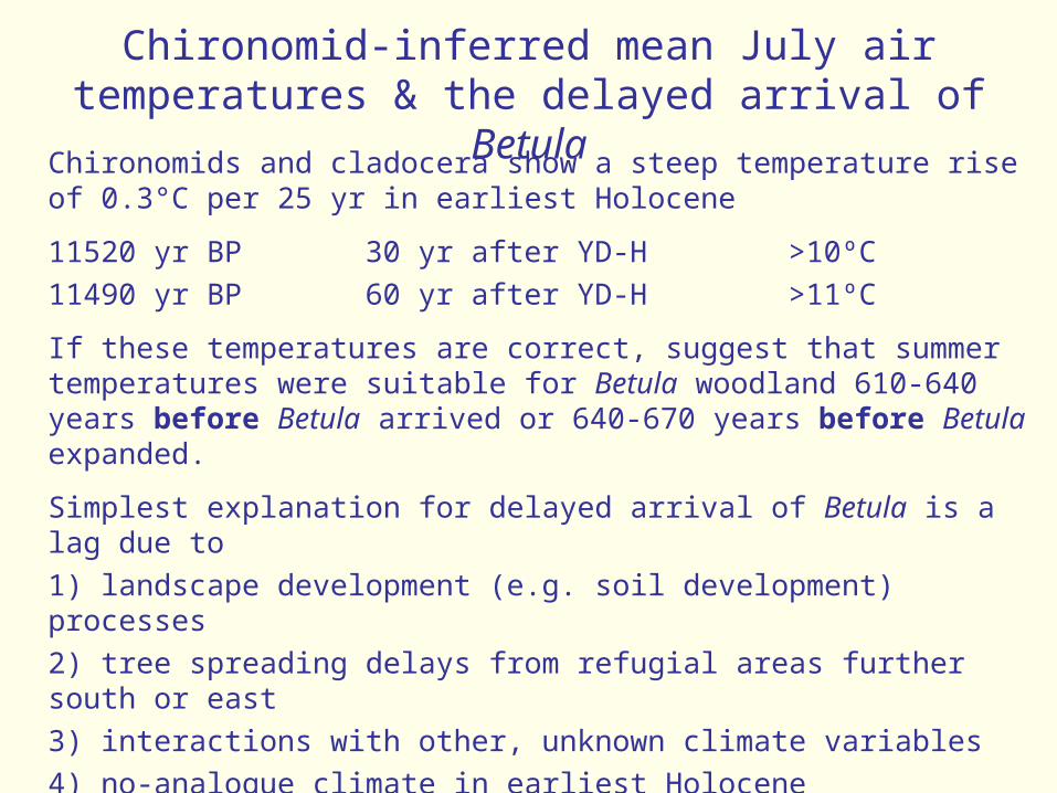
Chironomid-inferred mean July air temperatures & the delayed arrival of Betula
Chironomids and cladocera show a steep temperature rise of 0.3°C per 25 yr in earliest Holocene
11520 yr BP 30 yr after YD-H >10ºC11490 yr BP 60 yr after YD-H >11ºC
If these temperatures are correct, suggest that summer temperatures were suitable for Betula woodland 610-640 years before Betula arrived or 640-670 years before Betula expanded.
Simplest explanation for delayed arrival of Betula is a lag due to1) landscape development (e.g. soil development) processes2) tree spreading delays from refugial areas further south or east3) interactions with other, unknown climate variables4) no-analogue climate in earliest Holocene5) surprising amount of macroscopic charcoal suggesting local fires in the early Holocene (zone 6 – Empetrum zone)6) interactions of some or all these factors
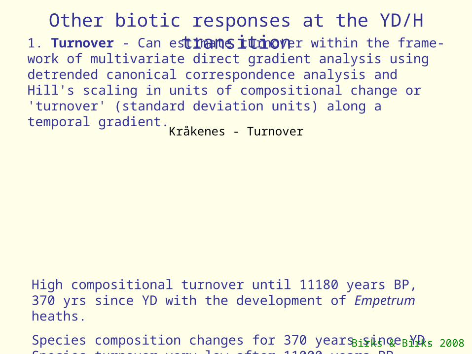
1. Turnover - Can estimate turnover within the frame-work of multivariate direct gradient analysis using detrended canonical correspondence analysis and Hill's scaling in units of compositional change or 'turnover' (standard deviation units) along a temporal gradient.
9000 9500 10000 10500 11000 11500 12000
0.0
1.0
2.0
3.0
Age (calibrated years BP)
Turn
over
(SD
uni
ts)
Krakenes - Beta Diversity
High compositional turnover until 11180 years BP, 370 yrs since YD with the development of Empetrum heaths.
Species composition changes for 370 years since YD. Species turnover very low after 11000 years BP.
Other biotic responses at the YD/H transition
Kråkenes - Turnover
Birks & Birks 2008
9000 9500 10000 10500 11000 11500 12000
0.0
0.1
0.2
0.3
0.4
0.5
0.6
Age (calibrated years BP)
Rat
e of
cha
nge
per 2
0 ye
ars
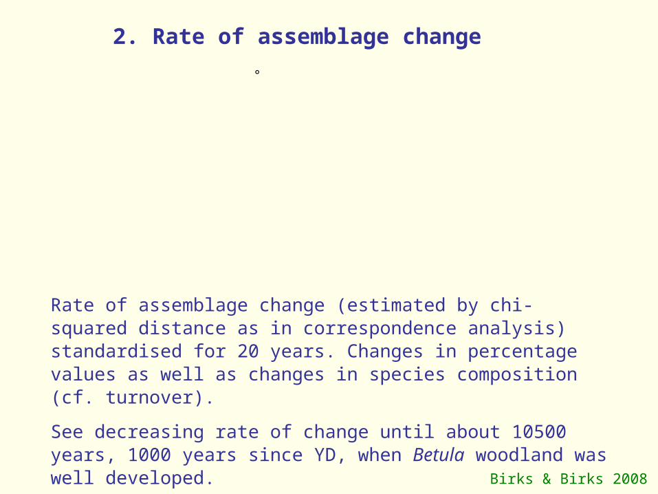
Krakenes - Rate of Change°
Rate of assemblage change (estimated by chi-squared distance as in correspondence analysis) standardised for 20 years. Changes in percentage values as well as changes in species composition (cf. turnover).
See decreasing rate of change until about 10500 years, 1000 years since YD, when Betula woodland was well developed.
2. Rate of assemblage change
Birks & Birks 2008
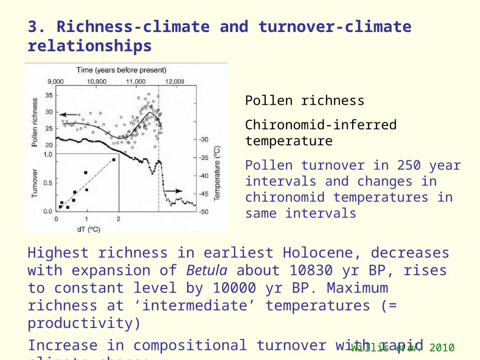
3. Richness-climate and turnover-climate relationships
Pollen richness
Chironomid-inferred temperature
Pollen turnover in 250 year intervals and changes in chironomid temperatures in same intervals
Highest richness in earliest Holocene, decreases with expansion of Betula about 10830 yr BP, rises to constant level by 10000 yr BP. Maximum richness at ‘intermediate’ temperatures (= productivity)
Increase in compositional turnover with rapid climate change Willis et al. 2010
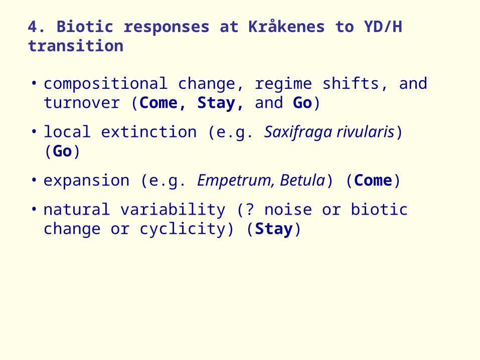
4. Biotic responses at Kråkenes to YD/H transition
• compositional change, regime shifts, and turnover (Come, Stay, and Go)
• local extinction (e.g. Saxifraga rivularis) (Go)
• expansion (e.g. Empetrum, Betula) (Come)
• natural variability (? noise or biotic change or cyclicity) (Stay)
What can Determine Stay or Go in the Past?
Ecological thresholds where an ecosystem switches from one stable regime state to another, usually within a relatively short time-interval (regime shift), can be recognised in palaeoecological records.
Much information potentially available from palaeoecological records on alternative stable states, rates of change, possible triggering mechanisms, and systems that demonstrate resilience to thresholds.
Key questions are what combination of environmental variables result in a regime shift and what impact does it have on biodiversity?
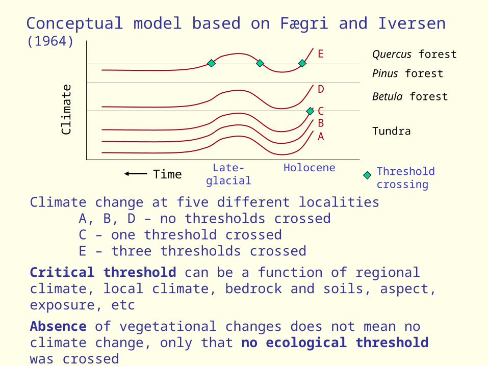
Conceptual model based on Fægri and Iversen (1964)
Clim
ate
TimeLate-glacial Holocene
Pinus forest
Betula forest
Tundra
Threshold crossing
Climate change at five different localitiesA, B, D – no thresholds crossedC – one threshold crossedE – three thresholds crossed
Critical threshold can be a function of regional climate, local climate, bedrock and soils, aspect, exposure, etc
Absence of vegetational changes does not mean no climate change, only that no ecological threshold was crossed
Stay or Go depends on thresholds being or not being crossed
A
E
D
CB
Quercus forest
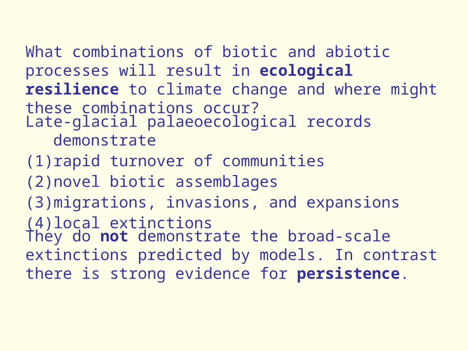
What combinations of biotic and abiotic processes will result in ecological resilience to climate change and where might these combinations occur?
Late-glacial palaeoecological records demonstrate (1) rapid turnover of communities(2) novel biotic assemblages(3) migrations, invasions, and expansions(4) local extinctions
They do not demonstrate the broad-scale extinctions predicted by models. In contrast there is strong evidence for persistence.

Palaeoecological data suggest that
1. rapid rates of spread of some taxa
2. realised niche broader than those seen today
3. landscape heterogeneity in space and time, and
4. the occurrence of many small populations in locally favourable habitats (microrefugia)
might all have contributed to persistence during the rapid climate changes at the onset of the Holocene
665
670
675
680
685690
695
700
705
710
715
720
725
730735
740
745
750
755
760
765
770
Dep
th (c
m)
20 40
Saxifraga
rivul
aris
20 40
Coc
hlear
ia
Saxifraga
cesp
itosa
Ran
unculu
s gl
acia
lis
Papaver s
ect. Scap
if lor
a
Cer
astiu
m a
rcti c
um
Juncus
t rig
lum
is t y
pe
Koenigia
islandica
500 1000 1500
Salix h
erbace
a leave
s
20 40
Salix p
olaris
leave
s
20
Sagina
inte
rmed
ia ty
pe
20
Oxy
ria d
igyna
20
Sedum ro
sea
20
Polygo
num v
ivipa
rum
bulbi
l
20
Luzula
undif
f.
EH
YD
Extinctions Expansions
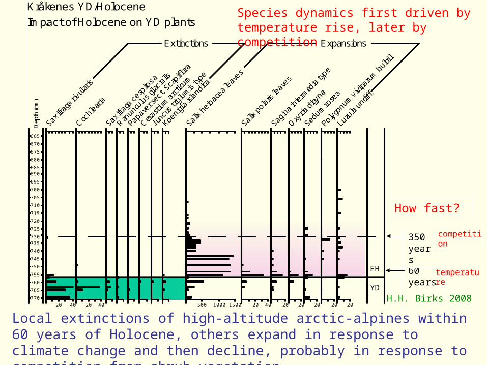
Kråkenes YD/Holocene
Impact of Holocene on YD plantso
60 years
350 years
Species dynamics first driven by temperature rise, later by competition
How fast?
temperature
competition
Local extinctions of high-altitude arctic-alpines within 60 years of Holocene, others expand in response to climate change and then decline, probably in response to competition from shrub vegetation.
H.H. Birks 2008
How can Q-Time Insights Contribute to Stay or Go?
Long thought that major last glacial maximum refugia for plants and animals were confined to southern Europe (Balkans, Iberia, Italian peninsula).
Now increasing evidence for tree taxa in microrefugia elsewhere in Europe. These microrefugia may have moved in response to climate change during last glacial stage – may explain why there may be a lag of 670 yrs at Kråkenes but almost no lag somewhere else in Betula expansion. Considerable stochasticity.Scattered microrefugia similar to concept of metapopulations in population biology – discrete but with some connectivity and dynamic.

LGM classical view - Traditional refugium model – narrow tree belt in S European mountains and in Balkan, Italian, and Iberian peninsulas
LGM current view - Current refugium model – scattered tree populations in microrefugia in central, E, and N Europe
Birks & Willis 2008

What Might LGM Microrefugia Have Looked Like?
Picea crassifolia, Sichuan 3600 mPicea <3%Artemisia and Poaceae >75%John Birks unpublished
Picea glauca, Alaska
Picea <1%Petit et al. 2008
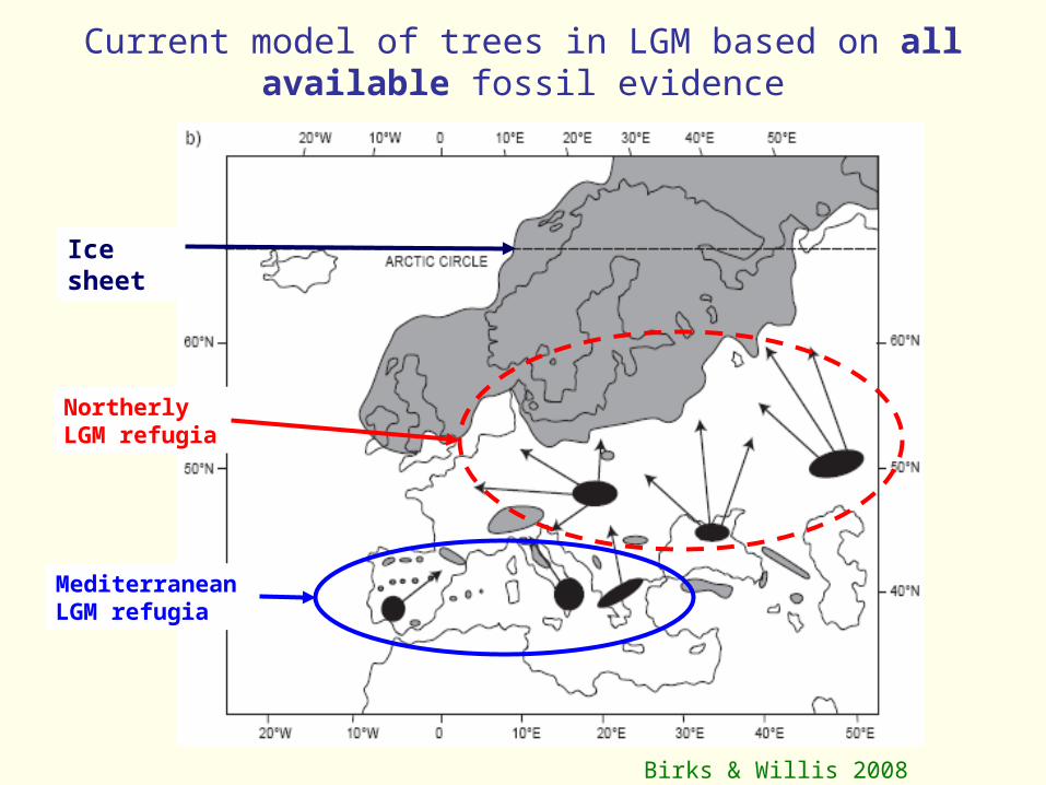
MediterraneanLGM refugia
Northerly LGM refugia
Ice sheet
Birks & Willis 2008
Current model of trees in LGM based on all available fossil evidence
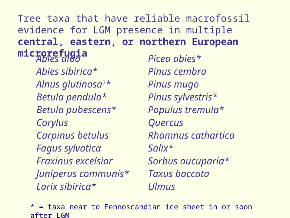
Tree taxa that have reliable macrofossil evidence for LGM presence in multiple central, eastern, or northern European microrefugia
Abies alba Picea abies*Abies sibirica* Pinus cembraAlnus glutinosa?* Pinus mugoBetula pendula* Pinus sylvestris*Betula pubescens* Populus tremula*Corylus QuercusCarpinus betulus Rhamnus catharticaFagus sylvatica Salix*Fraxinus excelsior Sorbus aucuparia*Juniperus communis* Taxus baccataLarix sibirica* Ulmus
* = taxa near to Fennoscandian ice sheet in or soon after LGM
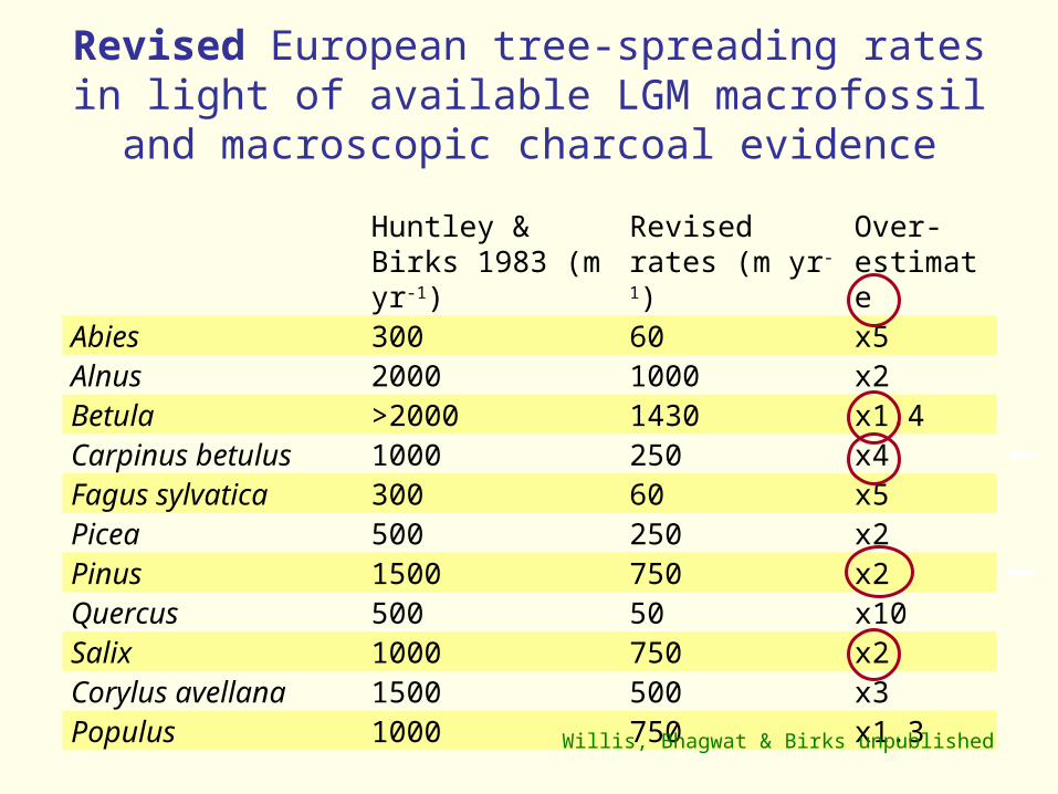
Revised European tree-spreading rates in light of available LGM macrofossil and
macroscopic charcoal evidence
Huntley & Birks 1983 (m yr-1)
Revised rates (m yr-1)
Over-estimate
Abies 300 60 x5Alnus 2000 1000 x2Betula >2000 1430 x1.4Carpinus betulus 1000 250 x4Fagus sylvatica 300 60 x5Picea 500 250 x2Pinus 1500 750 x2Quercus 500 50 x10Salix 1000 750 x2Corylus avellana 1500 500 x3Populus 1000 750 x1.3
Willis, Bhagwat & Birks unpublished

Isopollen mapping for Europe
Suggests spreading rates of 200-300 m yr-1
Huntley & Birks 1983

Is There Other Evidence for Microrefugia?
Palaeobotanical and Molecular Data Combined ‘The Way Forward in Palaeoecology’
Fagus sylvatica
Combination of palaeobotanical and molecular data
408 pollen sites with 14C dates
80 macrofossil sites
468-600 sites for chloroplast DNA and nuclear genetic markers (isozymes)
Magri et al. 2006 New Phytologist 171: 199-221
Jackson 2006 New Phytologist 171: 1-3
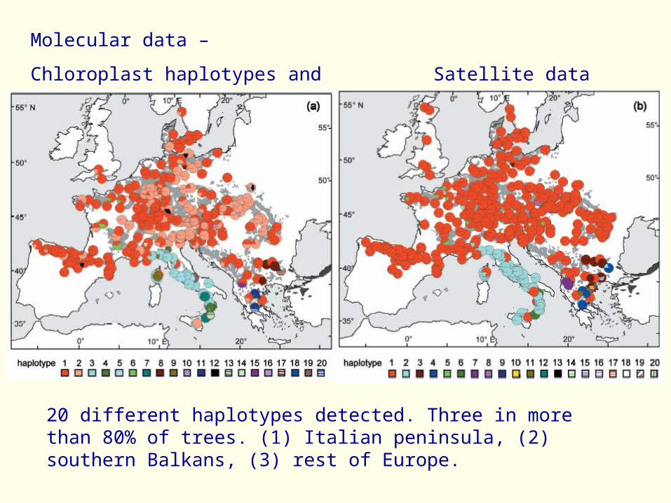
Molecular data –
Chloroplast haplotypes and Satellite data
20 different haplotypes detected. Three in more than 80% of trees. (1) Italian peninsula, (2) southern Balkans, (3) rest of Europe.

Nuclear genetic markers (isozymes)
Isozyme data – 9 groups
Italian group,
southern Balkans,
Iberian Peninsula,
rest of Europe

= >2% = macrofossil
Palaeobotanical data (pollen and macrofossils)
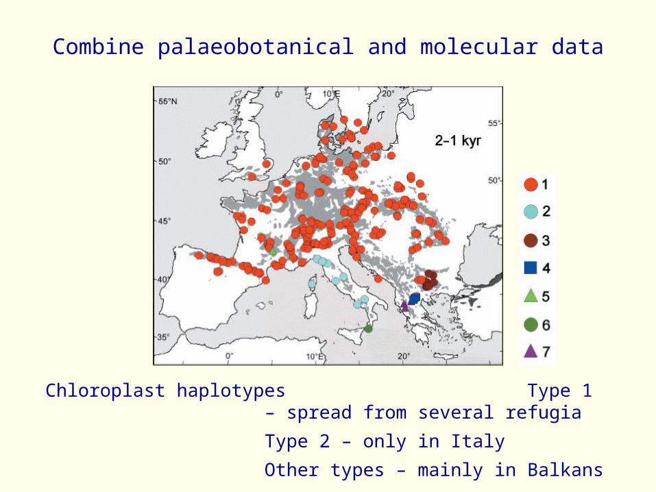
Combine palaeobotanical and molecular data
Chloroplast haplotypes Type 1 – spread from several refugia
Type 2 – only in Italy
Other types – mainly in Balkans

Isozyme groups
Type 1 – spread from several refugia
Type 9 – only in Italy
Type 7 – mainly in Balkans
Type 5 - Iberia
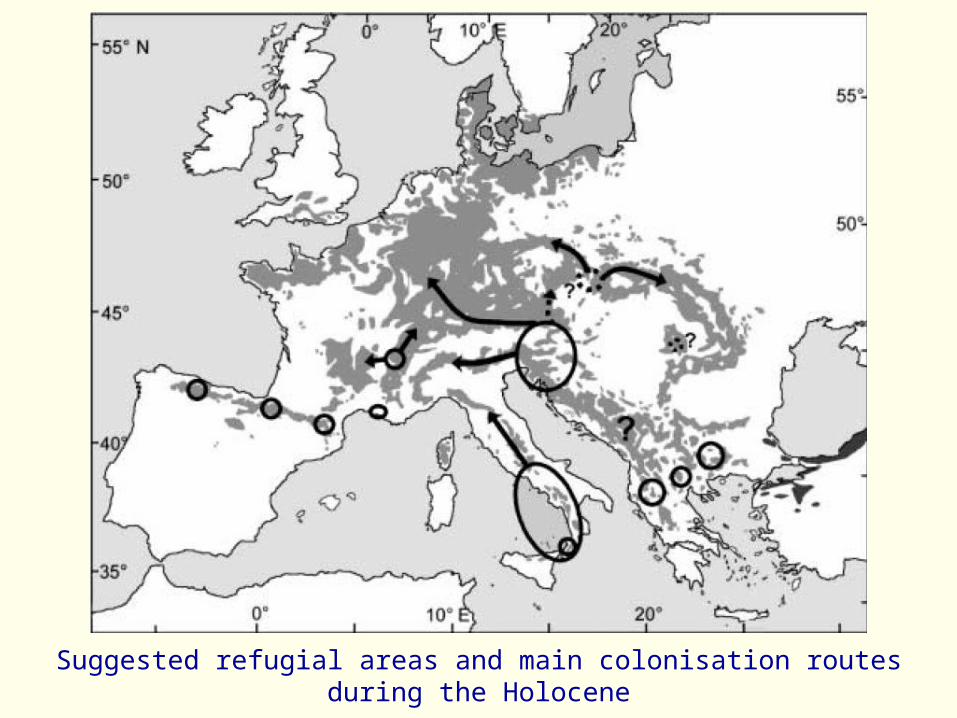
Suggested refugial areas and main colonisation routes during the Holocene
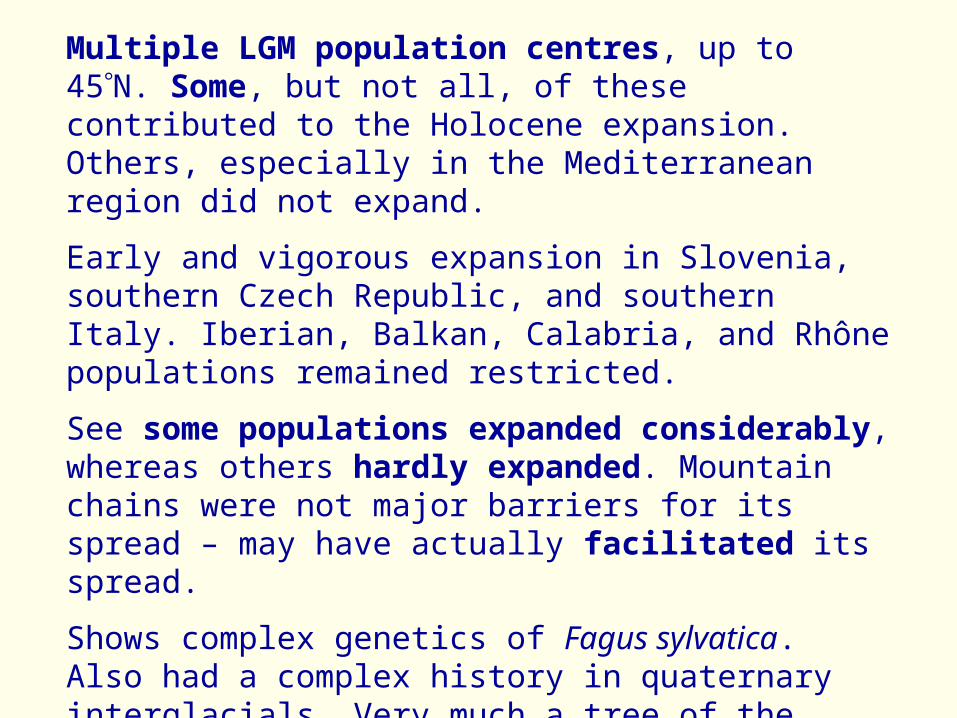
Multiple LGM population centres, up to 45N. Some, but not all, of these contributed to the Holocene expansion. Others, especially in the Mediterranean region did not expand.
Early and vigorous expansion in Slovenia, southern Czech Republic, and southern Italy. Iberian, Balkan, Calabria, and Rhône populations remained restricted.
See some populations expanded considerably, whereas others hardly expanded. Mountain chains were not major barriers for its spread – may have actually facilitated its spread.
Shows complex genetics of Fagus sylvatica. Also had a complex history in quaternary interglacials. Very much a tree of the Holocene. Questions of adaptation arise.
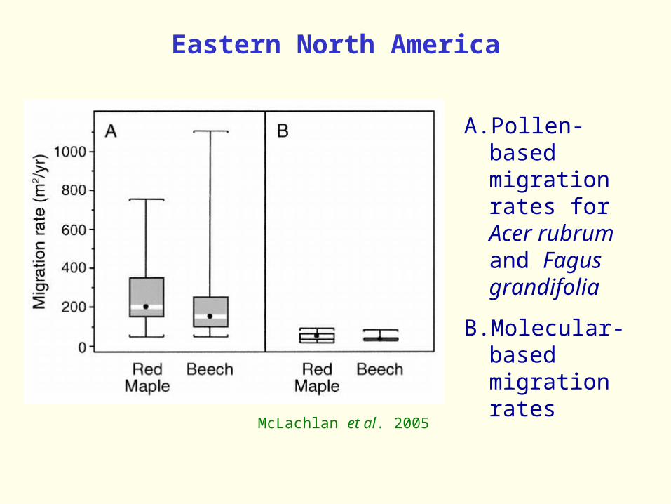
Eastern North America
A.Pollen-based migration rates for Acer rubrum and Fagus grandifolia
B.Molecular-based migration rates
McLachlan et al. 2005

Pinus
Quercus
Fagus
Ulmus
Corylus
Alnus
Pistacia
Tilia
Betula
Abies
Birks & Willis unpublished
Possible scenarios for earliest Holocene based on available palaeobotanical data
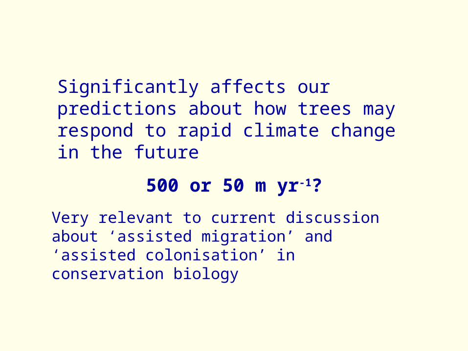
Significantly affects our predictions about how trees may respond to rapid climate change in the future
500 or 50 m yr-1?
Very relevant to current discussion about ‘assisted migration’ and ‘assisted colonisation’ in conservation biology
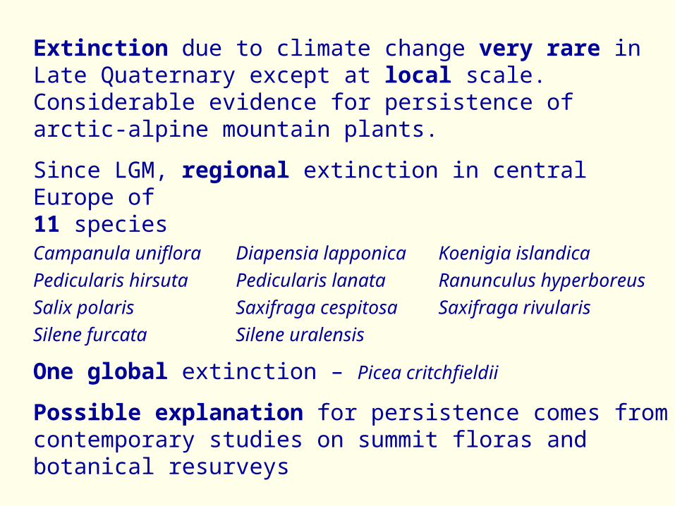
Extinction due to climate change very rare in Late Quaternary except at local scale.Considerable evidence for persistence of arctic-alpine mountain plants.
Since LGM, regional extinction in central Europe of 11 speciesCampanula uniflora Diapensia lapponica Koenigia islandicaPedicularis hirsuta Pedicularis lanata Ranunculus hyperboreusSalix polaris Saxifraga cespitosa Saxifraga rivularisSilene furcata Silene uralensis
One global extinction – Picea critchfieldii
Possible explanation for persistence comes from contemporary studies on summit floras and botanical resurveys
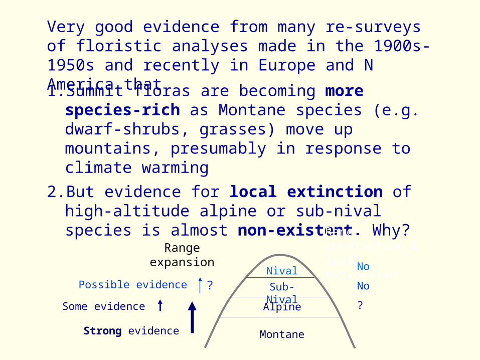
Very good evidence from many re-surveys of floristic analyses made in the 1900s-1950s and recently in Europe and N America that
1. Summit floras are becoming more species-rich as Montane species (e.g. dwarf-shrubs, grasses) move up mountains, presumably in response to climate warming
2. But evidence for local extinction of high-altitude alpine or sub-nival species is almost non-existent. Why?
Range expansionRange contraction & local extinction
Montane
Alpine
Sub-Nival
Nival?
No
No
?
Strong evidence
Possible evidence
Some evidence
Why is there little or no evidence for local extinction of high-altitude species?
Need to assess an alpine landscape not at a climate-model scale or even at the 2 m height of a climate station, but at the plant level.
Use thermal imagery technology to measure land surface temperature.
Körner 2007 Erdkunde
Scherrer & Körner 2010 Global Change Biology
Scherrer & Körner 2011 Journal of Biogeography
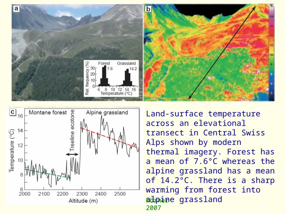
Land-surface temperature across an elevational transect in Central Swiss Alps shown by modern thermal imagery. Forest has a mean of 7.6°C whereas the alpine grassland has a mean of 14.2°C. There is a sharp warming from forest into alpine grasslandKörner 2007
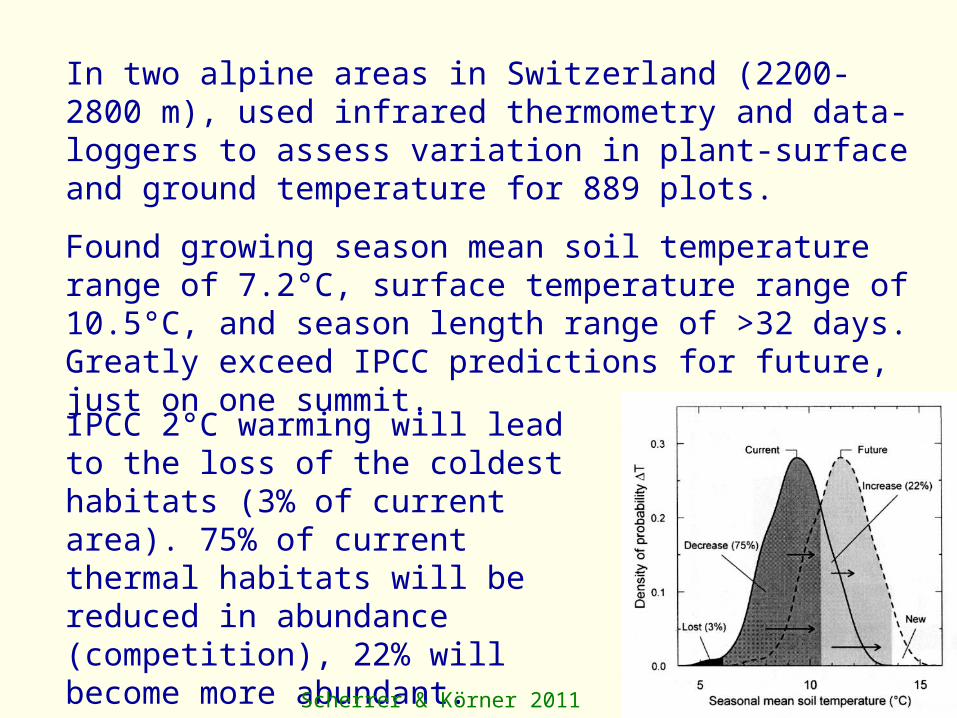
In two alpine areas in Switzerland (2200-2800 m), used infrared thermometry and data-loggers to assess variation in plant-surface and ground temperature for 889 plots.
Found growing season mean soil temperature range of 7.2°C, surface temperature range of 10.5°C, and season length range of >32 days. Greatly exceed IPCC predictions for future, just on one summit.
IPCC 2°C warming will lead to the loss of the coldest habitats (3% of current area). 75% of current thermal habitats will be reduced in abundance (competition), 22% will become more abundant.
Scherrer & Körner 2011
Warn against projections of alpine plant species responses to climate warming based on a broad-scale (10’ x 10’) grid-scale modelling approach.
Alpine terrain is, for very many species, a much ‘safer’ place to live under conditions of climate change than flat terrain which offers no short distance escapes from the new thermal regime.
Landscape local heterogeneity leads to local climatic heterogeneity which confers biological resilience to change.
What Conclusions can Q-Time Studies make to Stay and Go?
Biotic responses to major climatic changes in the Late quaternary have been mainly:
• distributional shifts (Go)
• high rates of population turnover (Stay)
• changes in abundance and/or richness (Stay)
• stasis (Stay)
Much less important have been
• extinctions (global, regional, or local)
• speciations (? any evidence except for micro-species in, for example, Primula, Alchemilla, Taraxacum, Meconopsis, Pedicularis, Calceolaria)

Biotic responses have been varied, dynamic, complex, and individualistic. Very difficult to make useful generalisations.
Important issues of spatial and temporal scales in bridging Q-time and Near-time studies.

As we move into the future, we need to predict what lies ahead. Just as early 17th century European map-makers applied for terra incognita the label ‘Here there may be dragons’, we should be aware that dragons may or may not lurk in our future.
However, whether dragons exist or not, we must consider all the data we have from Q-time and Near-time studies to ‘help future ecological predictions’ to avoid making too many incorrect predictions.
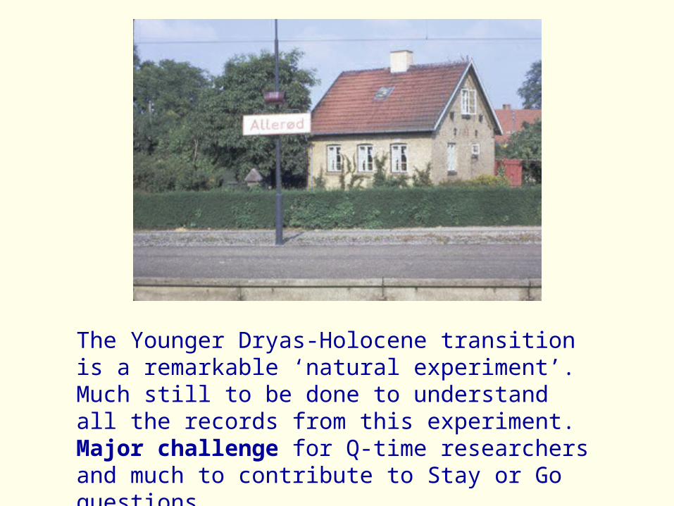
The Younger Dryas-Holocene transition is a remarkable ‘natural experiment’. Much still to be done to understand all the records from this experiment. Major challenge for Q-time researchers and much to contribute to Stay or Go questions.
Acknowledgements
Hilary Birks Kathy Willis
Sylvia Peglar Christian Körner
Steve Brooks Donatella Magri
Shonil Bhagwat Cathy Jenks