University of VermontScholarWorks @ UVM

Graduate College Dissertations and Theses Dissertations and Theses

2017

Status Monitoring Of Inflatables By Accurate ShapeSensingJustin Matthew BondUniversity of Vermont

Follow this and additional works at: https://scholarworks.uvm.edu/graddis

Part of the Mechanical Engineering Commons

This Thesis is brought to you for free and open access by the Dissertations and Theses at ScholarWorks @ UVM. It has been accepted for inclusion inGraduate College Dissertations and Theses by an authorized administrator of ScholarWorks @ UVM. For more information, please contactdonna.omalley@uvm.edu.

Recommended CitationBond, Justin Matthew, "Status Monitoring Of Inflatables By Accurate Shape Sensing" (2017). Graduate College Dissertations and Theses.677.https://scholarworks.uvm.edu/graddis/677

STATUS MONITORING OF INFLATABLES BY ACCURATE SHAPE SENSING

A Thesis Presented

by

Justin M. Bond

to

The Faculty of the Graduate College

of

The University of Vermont

In Partial Fulfillment of the Requirements

for the Degree of Master of Science

Specializing in Mechanical Engineering

January, 2017

Defense Date: November 7, 2016

Thesis Examination Committee:

Dryver R. Huston, Ph.D., Advisor

Ehsan Ghazanfari, Ph.D., Chairperson

Rachael Oldinski, Ph.D.

Cynthia J. Forehand, Ph.D., Dean of the Graduate College

ABSTRACT

The use of inflatable structures in aerospace applications is becoming increasingly

widespread. In order to monitor the inflation status and overall health of these inflatables,

an accurate means of shape sensing is required. To this end, we investigated two existing

methods for measuring simple curvature, or curvature in one-dimension. The first method

utilizes a pair of strain sensing Fiber Bragg Gratings (FBGs) separated by a known

distance; dividing the difference in strain by the separation distance yields an experimental

value for the one-dimensional curvature at a point. The second method makes use of

conductive ink-based flex sensors, which give a variable resistance based on curvature. We

used the latter was in a design for a Curvature-Based Inflation Controller (CBIC). While

the controller successfully inflated a test body, its overall utility is limited by the simplicity

of its sensors. To improve the shape sensing capabilities of the controller, we investigated

the use of FBGs in a multidimensional array.

We fabricated a curvature-sensing FBG pair on an inflatable membrane and tested

its accuracy as the membrane was shaped into a known radius of curvature. This work

reports on the assembly of three such curvature-sensing FBG pairs into a two-dimensional

Curvature-Sensing Rosette (CSR). The goal is to use this rosette to measure the curvature

of a surface in multiple directions at a single point. A 3-D printed surface with saddle

geometry was used to calibrate the curvature-sensing rosette. Presented will be methods of

extracting values for the tensor of curvature for the surface at a point using the curvature-

sensing rosette, along with experimental verification. This essentially defines the local

geometry about the rosette, measured in real time. By employing an array of such rosettes

across the surface of an inflatable structure, the local curvature of the inflatable could be

known at every point. Combining these curvature measurements can yield an accurate

depiction of the global geometry. Thus, the inflation status of the inflatable space structure

could be monitored in real time.

iii

TABLE OF CONTENTS

Page

LIST OF TABLES ........................................................................................................... v

LIST OF FIGURES ........................................................................................................ vi

CHAPTER 1: INTRODUCTION .................................................................................... 1

CHAPTER 2: CURVATURE IN ONE DIRECTION ..................................................... 9

2.1. The Geometry of a Space Curve ............................................................................ 9

2.2. Contemporary Methods for Sensing Curvature ................................................... 14

2.2.1. Fiber Bragg Gratings and the NASA Effort .................................................. 14

2.2.2. Conductive Ink-Based Flex Sensors .............................................................. 22

2.3. Controlling Inflation with Simple Curvature ....................................................... 26

2.3.1. Design Objectives and Theory ....................................................................... 26

2.3.2. Fabrication and Testing ................................................................................. 31

2.3.3. Results and Discussion .................................................................................. 33

CHAPTER 3: CURVATURE IN TWO DIRECTIONS ................................................ 37

3.1. The Geometry of a Surface .................................................................................. 37

3.2. Sensing Curvature in Two Directions.................................................................. 48

3.2.1. Design Objectives and Theory ....................................................................... 48

3.2.2. Fabrication and Testing ................................................................................. 54

3.2.3. Results and Discussion .................................................................................. 66

CHAPTER 4: CONCLUSIONS .................................................................................... 78

iv

REFERENCES .............................................................................................................. 82

APPENDIX .................................................................................................................... 84

v

LIST OF TABLES

Table Page

Table 1: FBG Bend Test Data ........................................................................................ 56

Table 2: FBG Bend Test Results ................................................................................... 56

Table 3: CSR Saddle Test Data ..................................................................................... 69

Table 4: CSR Saddle Test Results ................................................................................. 71

vi

LIST OF FIGURES

Figure Page

Figure 1: NASA Inflatable Antenna Experiment ............................................................ 2

Figure 2: NASA Hypersonic Inflatable Aerodynamic Decelerator ................................. 3

Figure 3: NASA Curvature Sensing Cable ...................................................................... 6

Figure 4: Geometry of a Space Curve ........................................................................... 10

Figure 5: FBG Operating Principle ................................................................................ 16

Figure 6: Effect of Strain on Wavelength ...................................................................... 18

Figure 7: Flex Sensor Made With Conductive Ink ........................................................ 23

Figure 8: Flex Sensor Behavior ..................................................................................... 24

Figure 9: CBIC Control Loop ........................................................................................ 28

Figure 10: CBIC Final Design ....................................................................................... 30

Figure 11: CBIC Inflation Test - Before and After ....................................................... 32

Figure 12: Hyperbolic Paraboloid .................................................................................. 39

Figure 13: Principal Curvature Examples ...................................................................... 45

vii

Figure 14: Rotation of Coordinate Axes ........................................................................ 50

Figure 15: CSR on Coordinate Axes ............................................................................. 52

Figure 16: FBG Bend Test Setup ................................................................................... 54

Figure 17: Bend Test Data ............................................................................................. 55

Figure 18: Curvature Sensing Rosette ........................................................................... 58

Figure 19: OSI Configuration Mode .............................................................................. 60

Figure 20: Virtual Saddle Surfaces in Solidworks ......................................................... 62

Figure 21: 3-D Printed Saddle Surfaces ........................................................................ 63

Figure 22: Male and Female Saddle Surfaces ............................................................... 63

Figure 23: The CSR on the Male Test Saddle ............................................................... 64

Figure 24: CSR and Saddle Pair Assembly ................................................................... 65

Figure 25: Data Acquisition for the CSR Test ............................................................... 66

Figure 26: Sample Data from the CSR Saddle Test ...................................................... 68

Figure 27: CSR Schematic Diagram .............................................................................. 70

Figure 28: Proposed CSR array ..................................................................................... 75

1

CHAPTER 1: INTRODUCTION

The field of space exploration has experienced significant growth in recent years.

Technological advances in the industry have nearly eliminated some of the barriers

traditionally associated with studying the cosmos. One of the most notable breakthroughs

has been the use of inflatable structures in space. The earliest inflatables were large

reflector dishes for antennae, and presented several inherent advantages over their rigid

metal counterparts [1]. For example, an inflatable space antenna reflector would naturally

weigh less, and could be stowed, uninflated, throughout the launching process. The

inflatable antenna could then easily survive the violent conditions of takeoff, which would

otherwise pose a quandary. In order to withstand the dynamics of a launch, most structures

intended for use in space would need to be separated into several smaller components, and

each of these would require its own launch vehicle, mission, etc. By employing inflatable

reflectors, however, researchers could send a probe with a compact antenna package into

space and then expand the inflatable reflector to be much larger than the vessel which

originally carried it. NASA’s Inflatable Antenna Experiment of 1996 shows this in the

figure below (Figure 1).

2

Figure 1: NASA Inflatable Antenna Experiment [2]

In the image above, the large silver reflector surface and the three beams connecting to it

were inflated after launch; the takeoff vessel only needed to be large enough to carry the

small copper-colored satellite. These inflatable antenna reflectors were first tested in the

1990s, and many are used to this day for the convenient advantages they provide.

More recently, inflatables have been tested for use in space applications as

aerodynamic decelerators and structural sections of space stations. NASA’s Hypersonic

Inflatable Aerodynamic Decelerator (HIAD) is showing promise as the next-generation

solution for atmospheric entry, and presents many attractive qualities over traditional

decelerators [3]. Just as the antenna reflector, an inflatable aerodynamic decelerator can

be stored for the takeoff and flight portions of a mission, then deploy for atmospheric entry.

The HIAD system developed by NASA can be seen in the figure below (Figure 2).

3

Figure 2: NASA Hypersonic Inflatable Aerodynamic Decelerator [4]

Beneath the grey heat-resistant fabric, there are several inflatable torus-like bodies, or

toroids. These concentric rings give the HIAD system its shape and structure, with many

reinforcing straps to improve rigidity. Again, this decelerator can inflate to be larger than

the landing vehicle, which is extremely beneficial to its utility. In fact, such an inflatable

would be critical to the objectives of the mission. Indeed, any mission involving an

inflatable structure would depend highly on the successful deployment of that inflatable

structure. Thus, obtaining an accurate depiction of the inflation process is particularly

important to the industry. It would allow mission controllers to monitor the status of the

inflatable and make vital decisions about the current mission.

Monitoring the progress of an inflating structure can be essential, but performing

such a task in space is inherently nontrivial. For instance, much of the inflating is

controlled remotely and without any visual cues present. Current methods of controlling

4

inflation utilize pressure measurements within the inflatable to determine the progress of

the inflation, but pressure readings alone are insufficient for assessing the process itself.

Such methods depend upon the inflation process to be smooth and without complication.

Were an issue to arise, such as unexpected entanglement of the uninflated body, a simple

pressure measurement would not identify the problem. In fact, the inflation process would

likely continue unabated, potentially causing catastrophic damage to the inflatable and

surrounding hardware. Given the nature of these missions, such a failure to diagnose an

inflation problem would certainly result in significant financial loss, in addition to months

of planning being wasted. Clearly, a more comprehensive method of monitoring inflation

is required.

In the absence of direct visual confirmation, a means of inferring the overall shape

and status of an inflatable could provide the feedback necessary to safely deploy an

inflatable. This is known as shape sensing, which is a method for detecting the geometry

of an inflatable body. Shape sensing utilizes sensors placed about the inflatable to monitor

the inflation status in real time. Because this method allows one to observe the geometry

of the body, any issues that might prevent the inflatable from successfully deploying would

be instantly identified. Moreover, once the structure was completely inflated, an accurate

shape sensing system would provide a means of health monitoring. For instance, any minor

deflection of a surface on the body due to debris impact or structural anomaly would be

quickly detected. Shape sensing can greatly reduce the risks associated with deploying

inflatable structures, which is why there have been significant efforts to investigate

practical methods of sensing shape.

5

One such effort has been made recently by researchers at NASA, led by Jason P.

Moore [5]. Using a chain of connected fiber optic strain gauges, called Fiber Bragg

Gratings (FBGs), they have developed a cable which measures curvature at numerous

points along its length. Curvature is a vector quantity that describes the degree and

direction to which an arc is curved. Mathematically, curvature is the inverse of the Radius

of Curvature, which is just the instantaneous radius required to produce the curve at a

particular point [6]. Engineers like Jason P. Moore are interested in measuring curvature

for its relationship to shape sensing: if the curvature of a body is known at a point, then the

local geometry about that point can be inferred. In order to fully specify the curvature of

a surface, three separate components must be measured. Assuming the curvature can be

found at many points about the body, the complete geometry of the inflatable can be

known. Or, by taking curvature measurements at specific points on the body, the inflation

status and shape can be monitored and controlled.

In the first portion of this investigation, a design for a novel inflation controller is

presented. Rather than relying on internal pressure readings, this device uses simple bend

sensors to detect the curvature at several points on the inflatable body. By using these

curvature readings as feedback, the Curvature-Based Inflation Controller (CBIC) is able to

successfully inflate an object to a desired level. Despite using a unique measure for its

feedback, this controller still suffers many of the pitfalls associated with traditional

pressure-based controllers. Chief among them is the necessity for the inflation process

itself to be spatially smooth and gradual. This is due to the nature of the curvature sensors

that were used; they can only measure simple curvature, or curvature in one direction. This

6

means that the final inflated geometry must be known, and all of the sensor data are merely

compared to the desired final values for curvature. The controller and sensor configuration

would thus need to be altered for every new inflatable geometry. In order to improve the

reliability and utility of the inflation controller, the sensors themselves would need to

become more sophisticated.

The NASA FBG chain is a powerful sensing system, capable of giving the operator

a clear view of the shape of the cable itself. However, just as the bend sensors used in the

CBIC, this fiber optic sensor bundle will only give the one-dimensional curvature at any

point. This is because the NASA cable is in essence a space curve. Space curves are one-

dimensional entities that exist in three-dimensional space [6]. The curvature sensing FBG

chain can be seen in the figure below (Figure 3).

Figure 3: NASA Curvature Sensing Cable [7]

The image above clearly shows the fiber optic cable in the lower left, and the computer

generated image of the cable’s shape on the monitor in the upper right. Because it is one-

7

dimensional, the curvature of such a space curve can only occur in one direction at a time.

This means that the NASA cable can only measure curvature in a single direction at a time.

The surface of an inflatable is a two dimensional body which exists in three-dimensions.

In order to completely define the geometry of a surface, additional curvature measurements

are required. In fact, the NASA cable is only able to provide an estimate of a surface’s

geometry when the FBG chain is run across the surface multiple times. The computer-

generated image then shows the path of the cable, with minor deflections, often due to twist

within the cable itself. While impressive, it is far from being capable of accurately

depicting the geometry of a two-dimensional surface. For this, a new type of curvature

sensor is required: one which can measure curvature in more than one direction at the same

time.

The second portion of this investigation was to design a sensor which could

accurately sense the shape of a surface by detecting curvature in more than one direction.

This new sensor would necessarily be an array of sensors which could each sense curvature

in a single direction. Fiber optic strain gauges were chosen for their high accuracy and

proven track record in the NASA FBG chain device, along with their small diameter and

sensing footprint geometry. A single pair of FBGs was combined into a curvature sensor,

and preliminary tests were performed. Once the method had been refined and results were

reliably accurate, an array of three curvature sensors was fabricated. The sensors were

placed in a classic strain rosette configuration; the two outer sensors were orthogonal to

each other, and the central sensor was aligned with the 45º angle between the other two.

In order to calibrate this new curvature sensor array, a custom saddle curve was designed

8

and 3-D printed. Male and female saddle profiles were fabricated to ensure the sensor

array would conform to the test surface of the saddle curve. Testing of this sensor array

proved successful; the new curvature sensor accurately detected the two-dimensional

curvature of the test surface. Such an array could be extremely useful in sensing the shape

of a surface, particularly that of an inflatable space structure. By placing these new sensors

at strategic points about an inflatable, the total geometry of the body could be known in

real time. Thus, the inflation status and overall health of an inflatable could be monitored

as necessary for mission success.

In the next chapter, the task of sensing curvature in one direction will be explored.

The mathematical definition of a space curve, as well as some contemporary methods for

detecting curvature will be discussed. Chapter 2 concludes with an in-depth analysis of

the inflation controller design and utility.

The third chapter examines the task of two-dimensional curvature detection and its

challenges. The properties of a surface will be defined mathematically. Finally, the novel

method of sensing curvature in multiple directions and its implications will be discussed.

9

CHAPTER 2: CURVATURE IN ONE DIRECTION

2.1. The Geometry of a Space Curve

In the context of shape sensing, detecting curvature on an inflatable surface is

essential. In order to discuss the various methods involved with sensing curvature, it is

necessary to fully define curvature as it applies to this topic. In this section, simple or one-

dimensional curvature will be discussed. This will involve delineation of the mathematical

quantity that is curvature as well as its significance in the real, physical world. As simple

curvature is primarily a property of space curves, the definition of a space curve will now

be presented.

A space curve is a continuous set of points existing in three-dimensional space [8].

Imagine a very thin wire that curves or bends through different angles and in different

directions, such that it cannot be confined to a plane. Although the wire itself has only one

dimension of significance, length, it still exists in three-dimensional space. This is, in

essence, the physical analog to the mathematical definition of a space curve. Now, let C

be a particular space curve in which we are interested. Assuming a Cartesian coordinate

system is present, then each point on C is defined by its position vector [8, 9]. This position

vector is denoted as 𝒙. The vector 𝒙 has components in the 𝒙1, 𝒙2, and 𝒙3 directions. The

following equation shows this [5].

𝒙(𝑢) = 𝑥1(𝑢)𝒆1 + 𝑥2(𝑢)𝒆2 + 𝑥3(𝑢)𝒆3 (1)

10

The terms 𝒆1, 𝒆2, and 𝒆3 are the unit normal vectors in the 𝒙1, 𝒙2, and 𝒙3 directions,

respectively. Note that 𝒙 and its components are all functions of the parameter 𝑢. This

can signify time, but not necessarily so; 𝑢 is simply a real variable associated with

increasing arc length along C [8]. The arc length along C will now be referred to as 𝑠. The

parameter 𝑠 has units of length and increases as 𝑢 increases. Refer to the following figure

for a visual representation of a space curve (Figure 4).

Figure 4: Geometry of a Space Curve

In the figure above, the curved red line represents the space curve, C. The position vector

𝒙 points from the origin to the curve, and 𝑠 increases along C from left to right in the figure.

The vector ∆𝒙 illustrates a change in position along C as 𝑢 increases, as if one were

11

traveling along the curve C. The following equation shows the change in 𝒙 and its

components with respect to a change in 𝑢:

Δ𝒙

Δ𝑢 =

Δ𝑥1

Δ𝑢𝒆1 +

Δ𝑥2

Δ𝑢𝒆2 +

Δ𝑥3

Δ𝑢𝒆3 (2)

Now, taking the limit of the above equation as ∆𝑢 goes to zero yields the following

differential representation of a changing position vector along C with respect to 𝑢:

𝑑𝒙

𝑑𝑢 =

𝑑𝑥1

𝑑𝑢𝒆1 +

𝑑𝑥2

𝑑𝑢𝒆2 +

𝑑𝑥3

𝑑𝑢𝒆3 (3)

The above quantity, 𝑑𝒙/𝑑𝑢, can be thought of as the average velocity of a body moving

along C. Although it does not explicitly depend on the arc length 𝑠, it can be rewritten as

follows:

𝑑𝒙

𝑑𝑢 =

𝑑𝒙

𝑑𝑠

𝑑𝑠

𝑑𝑢 = 𝒕

𝑑𝑠

𝑑𝑢 (4)

Here, the symbol 𝒕 denotes the unit tangent vector, which is the derivative of the position

vector with respect to arc length. The tangent vector is shown in (Figure 4), and always

points in the direction of increasing arc length. By definition, it is perpendicular to the

instantaneous radius of curvature, 𝜌. This radius of curvature always points in the direction

12

of the principal normal, or 𝒏 in (Figure 4) [6, 8, 9]. The principal normal points towards

the center of curvature and is of unit length.

Together, the principal normal and the tangent vector define the osculating plane

[6, 9]. This is the plane in which the osculating circle is found. The osculating circle is a

virtual circle which shares the same center and instantaneous radius of curvature as a point

on C. The orientation of the osculating plane therefore changes with the orientation of the

osculating circle. Imagine C in the figure curving towards the negative 𝒙3 direction, as

shown, and then turning back upwards towards the positive 𝒙3 direction. This would cause

the direction of 𝒏, which lies in the osculating plane and points towards the center of the

osculating circle, to flip about C when the direction of the curve changes. This relationship

is imperative to understanding one-dimensional curvature, because the curvature vector

always points in the direction of the principal normal.

Recall that the tangent vector is the derivative of the position vector with respect to

arc length. Taking the second derivative with respect to arc length yields the curvature

vector, or 𝜿. The curvature is shown in (Figure 4), and its mathematical definitions are

shown below.

𝜿 =

𝑑𝒕

𝑑𝑠 =

𝑑2𝒙

𝑑𝑠2 (5)

𝜅 𝒏 =

𝑑𝑡

𝑑𝑠 𝒏 (6)

𝜅 =

1

𝜌 (7)

13

As stated, the curvature vector is the derivative of the tangent vector with respect to arc

length, and the second derivative of the position vector with respect to arc length. The

scalar quantity of curvature is simply 𝜅 and is the inverse of the instantaneous radius of

curvature. The scalar 𝜅 can be thought of as a measure of the degree to which C is curving.

Essentially, it is the rate of change of the tangent vector as it travels along C in the direction

of increasing 𝑢. The curvature vector will always point in the same direction as the curve

itself, or the same direction as the principal normal.

This relationship between curvature vector and the curve itself is critical to the

utility of a curvature measurement for the purposes of shape sensing. If both the curvature

direction and magnitude are known at a point on an inflatable, then the profile of the local

area about that point can be estimated. This is the strategy employed by NASA’s FBG

chain, which will be discussed at length in the coming section. By taking curvature

measurements at many points on the inflatable surface, the entire profile can be interpolated

and thus defined, to a certain degree of accuracy. Of course, the accuracy of this method

could be improved by placing more sensors in the same space and thereby reduce the

amount of error present due to interpolation. Additionally, more sensors could be placed

at specific points of interest across the body, such as a point of a mounting interface. This

would be similar to the practice of increasing the density of finite elements around points

of high stress concentration or complex geometry when performing finite element analysis.

When employed properly, the curvature readings from the surface of an inflatable can

become a powerful means of sensing its shape.

14

At this point, it is important to reiterate that the curvature quantity discussed above

is a vector, which points in a single direction by definition. This is due to the nature of the

curve itself; it only possesses a single dimension, length, and thus can only experience

curvature in one direction at a time. Regardless of the direction or degree to which C is

curving, at each individual point along C, the curvature is only ever a vector which acts

along a single direction. This means that any method which utilizes simple curvature

measurements would only capture a single profile or cross section of the total surface. An

inflatable body’s surface is after all two-dimensional, and additional sensors would need

to be placed in multiple directions to detect the curvature in more than one dimension. This

will prove to be the motivation for the second part of this investigation, which will be

discussed in subsequent sections.

2.2. Contemporary Methods for Sensing Curvature

2.2.1. Fiber Bragg Gratings and the NASA Effort

One of the most accurate means of sensing curvature with intrinsic embedded

sensors, available today, involves the use of fiber optic strain gages, also known as Fiber

Bragg Gratings. These are sections in a fiber optic cable which have been specially treated

to exhibit different refractive properties than the rest of the cable. A length of fiber, which

is made of glass, has a certain refractive index associated with its optical density. The

variation of refractive index with radial position is the reason why fiber optic cables are

able to transmit data; the interior index is so high that complete internal reflection occurs

along the length of the fiber. So, if a light source enters one end of the fiber, it will reach

the far end of the fiber with minimal loss of intensity. Some loss may occur around tight

15

bends in the cable, as these essentially reduce the angle required for the light to be

transmitted out of the surface of the fiber.

Typically, it is desirable for the refractive indices of the various layers of a fiber to

be uniform along the length. Any deviation would be viewed as a defect in the fiber.

However, in an FBG, the refractive index of the core is intentionally altered to create

regions of higher optical density. There are several methods for fabricating FBGs, but all

of them make use of UV light to alter the refractive index of the fiber [10]. During the

manufacturing process, the center of a fiber is doped with a photosensitive compound.

These doping compounds typically include Germanium and cause the center of the fiber to

be sensitive to permanent change via UV radiation [10, 11]. Holographic or interferometric

methods will split UV laser light into two separate beams, and then recombine them to

produce an interference pattern on the fiber [10]. This pattern, often comprising thousands

of fringes, reacts with the doping compound within the fiber. Any region of the fiber

exposed to the UV light has its refractive index permanently altered [10, 11]. The spacing

of these regions can be adjusted by changing the interference pattern. Other,

noninterferometric, methods make use of periodic pulses of UV light, or shine UV light

through a specially designed phase mask to activate the doping compound within the fiber

and produce the desired regions of high optical density. A grating is a collection of many

such regions; when the spacing of these regions is chosen to correspond with a specific

wavelength, it is known as a Fiber Bragg Grating [10, 11]. When a spectrum of light is

shown on one end of the fiber containing an FBG, this predetermined wavelength, known

16

as the Bragg wavelength, will be reflected back to the source end. The following figure

gives a depiction of this process (Figure 5).

Figure 5: FBG Operating Principle [12]

Note that the reflected peak is returned to the end of the fiber into which the incident

spectrum is shown. This means that only one end of the fiber need be connected to an

interrogating device, a particularly useful characteristic for remote sensing of structures or

inflatables. The peak in the above graphic shows the Bragg wavelength (𝜆B), which is

related to the fringe spacing (Λ) within the grating by the following equation:

𝜆𝐵 = 2𝑛Λ (8)

In this equation, 𝑛 signifies the effective index of refraction of the grating. This

refractive index is subject to change with the conditions affecting the fiber [13].

17

Specifically, if the FBG experiences a mechanical strain or a change in temperature, the

effective index of refraction will change. This change can be quantified, and thus the strain

or temperature variance can be measured. The following equation gives the relationship

between wavelength shift (∆𝜆/𝜆𝑜) and strain (𝜀) and temperature change (∆𝑇).

Δ𝜆

𝜆𝑜 = 𝑘 𝜀 + 𝛼𝛿 ∆𝑇 (9)

The 𝑘 term is known as the gauge factor, and is generally approximately 0.78. The gauge

factor is a constant which allows one to determine the strain associated with a change in

wavelength. The term 𝛼𝛿 is the change in refractive index with respect to temperature.

Although the temperature sensing capabilities of FBGs are impressive, they are not

included in this study. This essentially means that the term on the far right of the above

equation can be neglected. That term applies to the change in refractive index, and thus

wavelength, caused by the temperature change. Provided there is no temperature change

during the straining process, then there is no effect on the wavelength. It should be noted

that the strain term above is actually a combination of mechanically caused strain and strain

due to temperature change [14]. Not only does the index change due to mechanical strain,

but as the temperature of the FBG changes, it undergoes thermal expansion or contraction.

This accounts for an additional strain contribution, which can complicate attempts to

measure purely mechanical strain. Fortunately, just as the thermal effects on the refractive

index, as long as the temperature change is insignificant, then so are its effects on the

18

wavelength shift. Without the impact of temperature, the only factor influencing

wavelength shift is the mechanical strain, which is illustrated in the figure below (Figure

6).

Figure 6: Effect of Strain on Wavelength [15]

This figure demonstrates the reflected peak, which is the Bragg wavelength, shifting to a

longer wavelength as the FBG is stretched. The reverse is also true; as the FBG is

compressed, the peak will shift towards a shorter wavelength, resulting in a negative value

for the calculated shift. By measuring this shift, one can determine the amount of strain

present in the fiber.

Obtaining a measure of the curvature from FBGs is directly related to measuring

the strain. In fact, a curvature reading simply requires two FBGs on either side of the curve

and a known separation distance. Imagine a beam that is bending with one FBG on the

outside of the bend, and another on the inside. The outer FBG will be in tension, while the

inner FBG will be in compression. This will result in a positive strain for the FBG in

19

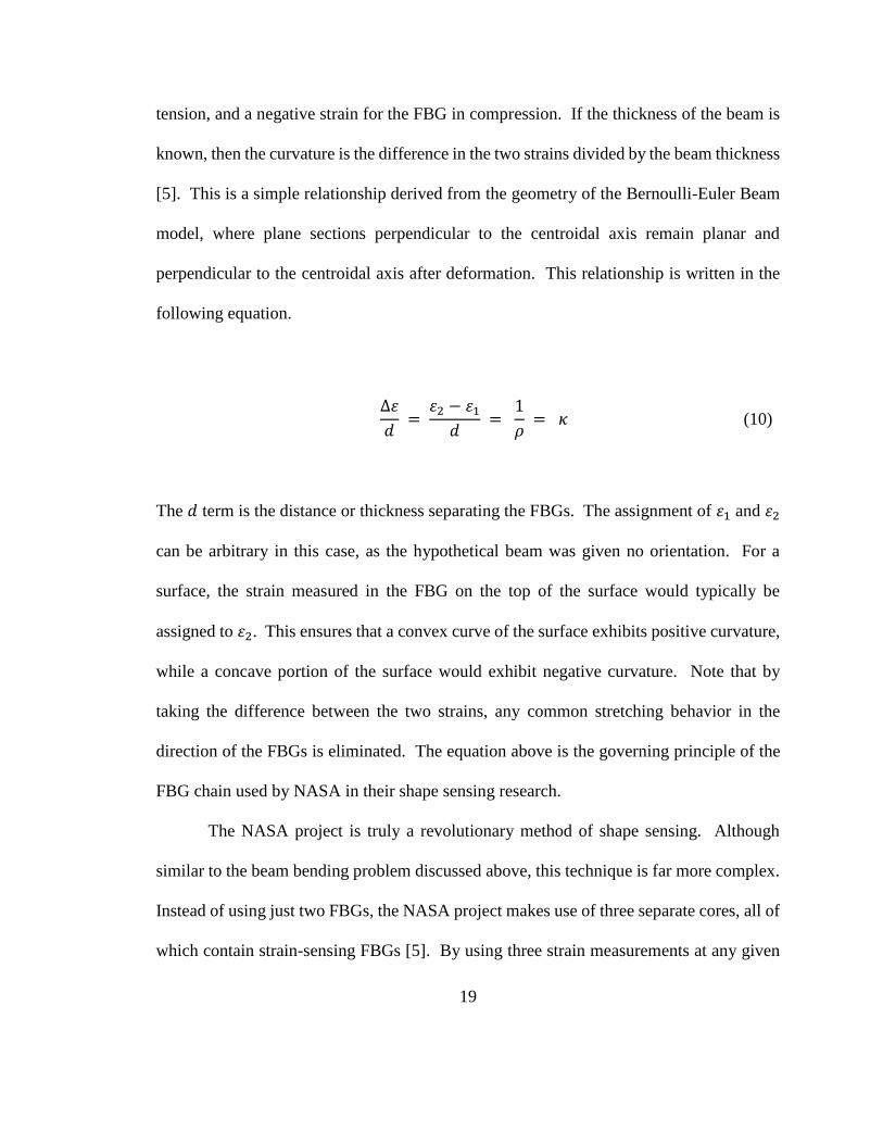
tension, and a negative strain for the FBG in compression. If the thickness of the beam is

known, then the curvature is the difference in the two strains divided by the beam thickness

[5]. This is a simple relationship derived from the geometry of the Bernoulli-Euler Beam

model, where plane sections perpendicular to the centroidal axis remain planar and

perpendicular to the centroidal axis after deformation. This relationship is written in the

following equation.

Δ𝜀

𝑑 =

𝜀2 − 𝜀1

𝑑 =

1

𝜌 = 𝜅 (10)

The 𝑑 term is the distance or thickness separating the FBGs. The assignment of 𝜀1 and 𝜀2

can be arbitrary in this case, as the hypothetical beam was given no orientation. For a

surface, the strain measured in the FBG on the top of the surface would typically be

assigned to 𝜀2. This ensures that a convex curve of the surface exhibits positive curvature,

while a concave portion of the surface would exhibit negative curvature. Note that by

taking the difference between the two strains, any common stretching behavior in the

direction of the FBGs is eliminated. The equation above is the governing principle of the

FBG chain used by NASA in their shape sensing research.

The NASA project is truly a revolutionary method of shape sensing. Although

similar to the beam bending problem discussed above, this technique is far more complex.

Instead of using just two FBGs, the NASA project makes use of three separate cores, all of

which contain strain-sensing FBGs [5]. By using three strain measurements at any given

20

point along the cable, this device can detect any direction of curve experienced by the cable.

Recall the beam example, which used only two FBGs. As long as the beam was bending

such that the FBGs were on either side of the curve, then those two would suffice.

However, if the beam were to bend in a new direction orthogonal to its original bend

direction, the two FBGs would no longer be on either side of the curve. Any curvature

associated with this in-plane bending of the beam would be impossible to detect with the

current configuration. This is why the NASA cable has three separate cores; regardless of

the bend direction, the curving behavior of the cable can always be captured. With the

curvature measured, one can essentially work backwards to determine the shape of the

cable. NASA uses similar equations to the ones introduced in the section of this paper

discussing space curves, known as the Frenet-Serret formulas, to perform these calculations

[5, 6]. This is how the NASA FBG chain can be used to generate a virtual image of the

cable itself. Thus, the FBG chain is capable of measuring a curve in any single direction,

and the only limitation on its accuracy in this respect is the number of FBGs along the

cable.

In order to place a large number of FBGs within the length of their cable, NASA

turned to a technique known as multiplexing. This is typically done to increase the number

of signals that can be sent through a fiber. A device called a multiplexer separates an

incident spectrum of light into specific wavelengths that are then shone into one end of the

fiber. On the far end of that same fiber, another device interrogates the now many

wavelengths of light and their associated data. This greatly increases the amount of

information that can be sent through a single fiber, which is why NASA chose to employ

21

this technique. Multiplexing with FBGs does not require an initial multiplexer, because

each FBG can be written to reflect a different wavelength. By writing many FBGs, each

with a unique wavelength, into a single fiber, the requirement of multiplexing is fulfilled

[13]. The resulting fiber can be thought of as a chain of FBGs. Not only does each FBG

measure strain independently of the others in the chain, but each unique wavelength

corresponds to the position along the curve at which that FBG can be found. The three

multiplexed FBG chains thus allow researchers at NASA to know both the location and

curvature of many points along the cable. This is why the computer generated image in

(Figure 3) looks nearly identical to the chain itself. It is a very powerful technique for

measuring curvature due to the high accuracy of the FBGs.

Despite the numerous advantages afforded by the NASA fiber optic cable, this

method is still limited in its shape sensing capabilities. Because the cable is in essence a

space curve, it can only ever experience curvature in one direction at a time. This means

it can only measure a single direction of curvature at a time. As previously stated, the

geometry of a surface cannot be captured by a single component of curvature. In order to

provide more than just a profile of the inflatable surface, the NASA FBG chain must weave

back and forth across an area multiple times. When the virtual image of the chain used in

this manner is generated, one can glean a general understanding of the surface geometry.

However, surface details are lost between the bends of the cable. Additionally, any

inaccuracies of the method, such as those caused by twist within the fiber, distort the image

created by the computer. Although recent developments suggest that NASA can now

account for twist within the cable, the underlying shortcomings of their shape sensing

22

method persist. This is due to the nature of the method itself. The fiber cable can sense its

own curvature very accurately, but this is not equivalent to the curvature of the surface

upon which it rests. While the cable method can provide a qualitative depiction of a

surface, it cannot be used to quantify the curvature of that surface. This requires a distinct

approach to the problem of shape sensing; one which measures the curvature of the surface

and not simply a space curve. With an accurate measure of the surface geometry at multiple

points about an inflatable, the geometry of the spaces between sensors could be inferred.

With the current NASA method, the regions in between cable runs are completely

unmeasured, and researchers can only guess as to their precise geometries.

A more comprehensive approach to shape sensing requires the measuring of three

components of curvature on the surface. This requires the fabrication of a novel sensor

array specifically designed to measure the curvature of a surface. With enough of these

new sensors placed about an object, the complete geometry can be known, and the inflation

process can be monitored. As a proof-of-concept exercise, an inflation controller was

designed to receive inputs in the form of curvature measurements and use them to control

the flow of air into an inflatable. In this preliminary study, the selected curvature sensors

were of the conductive ink type. These bend or flex sensors, as they are also known, are

discussed in the next section.

2.2.2. Conductive Ink Based Flex Sensors

Although the accuracy of FBGs makes them highly valued for shape sensing, an

economic alternative is the flex sensor. 2 This flexible potentiometer provides a variable

electrical resistance which depends on the amount of bend present in the body of the sensor.

23

The sensor body, or substrate, is made from a material which is both flexible and

electrically insulating [16]. A conductive ink is then applied to the substrate. Once dried,

this conductive ink becomes a connection between two electrical contacts. The figure

below shows a typical conductive ink type flex sensor with a loop of wire attached to its

contacts (Figure 7).

Figure 7: Flex Sensor Made With Conductive Ink [17]

As the substrate is bent, the conductive ink is strained longitudinally and experiences a

reduction in its cross sectional area. Moreover, the conductive ink begins to crack and

from gaps as it is deformed [16]. Both of these behaviors contribute to an increase in the

electrical resistance of the potentiometer. This change in resistance is proportional to the

amount of deflection of the substrate. The following figure shows three potential

configurations of a bend sensor and the associated changes in resistance (Figure 8).

24

Figure 8: Flex Sensor Behavior [18]

The process depicted above occurs in a predictable manner, and the resistance fluctuation

can be measured simply by applying a voltage across the two contacts.

In order to measure curvature using a flex sensor, one must calibrate each sensor

individually. This is because the exact process by which the conductive ink cracks and

deforms is unique to each sensor. A simple method of calibration employs test surfaces of

known curvature. With a known voltage applied, the flex sensor is shaped to fit the curved

surface, and the resulting voltage change is recorded. By performing this process for a

number of known curvature values, the flex sensor can be calibrated. A number of test

surfaces are required. While the resistance varies in a repeatable manner, it does not vary

linearly with the bending of the substrate. This necessity for individual calibration is one

of several disadvantages encountered with the use of flex sensors.

Another prominent shortcoming of the flex sensor is the nature of its variable

resistance. As the sensor is bent, the resistance change is a result of an average amount of

25

curvature present in the substrate. Depending on the surface which it measures, the

substrate could be severely bent on the end closest to the contacts and relatively flat on the

end furthest from the contacts. This would yield a specific increase in resistance, which

could then be measured. However, the exact same resistance change could be caused by

the reverse situation, with a flat portion near the contacts and a severe curve on the far end.

There is also a configuration in which the substrate experiences a consistent amount of

curvature which would yield the same exact resistance change. Thus, a simple voltage

drop caused by a flex sensor is not enough to define the curvature of a surface; it will only

give an average reading of the curvature in the substrate. Fortunately, this issue can be

largely overcome by choosing an appropriate size for the flex sensor. Due to its design,

the flexile potentiometer can be produced in a multitude of sizes. This allows one to select

a flex sensor which is relatively small when compared to the surface it will be measuring.

In this case, an average reading of curvature will likely be representative of the curve

present on the surface in the area immediately surrounding the flex sensor.

Another disadvantage comes from the fact that the flex sensor is once again a one-

dimensional curve. Just as the NASA cable, a flex sensor can only provide a reading of

curvature in a single direction. So once more, a new method of curvature must be

developed which captures the curvature of a surface, not just a space curve.

Despite these disadvantages, there are several reasons to justify the use of flex

sensors in shape sensing applications. For one, the flex sensor itself is relatively robust.

When compared to an FBG, the flex sensor substrate can withstand a far greater amount of

physical trauma that may occur during the inflation process. In addition, the average flex

26

sensor is far less expensive to manufacture when compared to an FBG. They are also

considerably easier to use in a controller application; flex sensors can be reduced to simple

analog voltage inputs whereas FBGs require sophisticated interrogation equipment and

software. For these reasons, the flex sensors were chosen for a prospective inflation

controller, which is the focus of the next section.

2.3. Curvature-Based Inflation Controller

2.3.1. Design Objectives and Theory

The current need for accurate shape sensing of inflatables is based on the notion

that an inflatable can be monitored and its inflation controlled. As a preliminary

investigation into this quandary of improving shape sensing, a Curvature-Based Inflation

Controller was designed. The goal of this CBIC was to serve as a proof of concept for the

potential application of a novel shape sensor. Successful operation of the inflation

controller would then justify additional study in the field of shape sensing.

The main objective of the controller was to autonomously inflate an initially

deflated body to desired final inflation level. This final inflation level would be measured

solely by sensing the shape of the inflatable, as opposed to using a pressure gauge or some

other technique. This distinction is important for two reasons; (1) for a successful design,

it would support the notion of using shape sensing, and (2) it makes this controller unique.

In order to use contemporary shape sensing methods as the only source of feedback,

several assumptions were necessary. First, it was assumed that the body in question

contained regions that could be described by the simple, one-dimensional, curvature. This

27

is because the current shape sensing techniques only allow for the measurement of one

direction of curvature at a time. This assumption is easily justified, as there are many

possible inflatable geometries which contain one or more regions characterized by a single

direction of curvature. Such regions are referred to as parabolic points, and will be

discussed further in the next chapter. However, a simple example of a parabolic region is

the side body of a cylinder. The only direction of curvature is in the plane of the

circumference of the cylinder. So, for this simple geometry, a single dimension of

curvature could suffice to sense its shape, assuming the body inflates uniformly, and no

unexpected bending or folding occurs. This is the essence of the second main assumption

for the controller design: that the inflation process itself is spatially smooth, and no

unexpected complications arise during inflation. Essentially, the inflation process must

occur such that the measured regions are initially flat, and gradually become more curved

as the body is inflated. The maximum curvature of these regions will be reached only when

the body is fully inflated, and not before. This also assumes that no portion of the body

will inflate more quickly than the rest, as this would again lead to curvature in more than

one direction at a time, which cannot be captured at present. With these assumptions

defined, the controller could be designed.

The first step in designing this inflation controller was the selection of the inflatable

object itself. A child-sized air mattress was chosen for its relatively simple geometry, ease

of inflation control, and low cost. For instance, the sides of the air mattress exemplify the

desired parabolic geometry. In addition, the internal structure of the mattress is somewhat

representative of that of inflatable space structures, with multiple chambers designed to

28

hold its shape. Finally, the material of the mattress is useful as it limits the amount of

stretching within the surface itself. While it is not fabric-reinforced as many inflatable

space structures are, the vinyl of the air mattress does not stretch in an appreciable amount

during the process of routine inflation. This is important, as the type of deformation of

interest is curvature, and excessive stretching could potentially skew sensor readings.

With the inflatable chosen, the selection of the remaining parts was relatively

straightforward. The choice of actuator, or air pump in this case, was obvious. The air

mattress was accompanied by a small air pump which could be plugged into a 120VAC

power supply. This pump would be operated by a relay, which would interrupt the power

going to the pump when the mattress was fully inflated.

The relay would then be controlled by a programmable Arduino board, which was

chosen for its ease of operation. The figure below shows the control loop used for the

design of the CBIC (Figure 9).

Figure 9: CBIC Control Loop

As shown on the left of the figure above, the control loops begins with the AC power

supply, in this case a wall outlet. The Arduino controller then operates the relay, which

allows the actuator, an air pump, to be powered. The plant is of course the air mattress,

29

which is inflated by the air pump. As the mattress inflates, the flex sensors detect the

curvature at specified points. The Arduino board then uses this sensor feedback to turn the

relay off once the desired level of inflation is achieved. Although not particularly powerful,

this Arduino board could be easily programmed to carry out the task of operating the relay

based on the shape sensor input. In a sense, the relatively minimal computing power of the

Arduino was ideal for demonstrating the overall simplicity of the CBIC. This simplicity is

surely a desirable attribute in space applications, where so many complex systems exist

and quantities like voltage and CPU usage are strictly rationed.

As previously stated, the shape sensing technique employed by the CBIC was the

flexible potentiometer, or bend sensor. These were chosen for both their durability and

availability. Given that the precise conditions of the inflation process are still largely

unknown, the plastic resin substrate of the flex sensors made them the conservative choice.

In addition, the flex sensor technology has existed for decades, making them widely

available and relatively low in cost. These factors made flex sensors the logical choice for

sensing curvature with the CBIC.

Once the control loop was designed, and the parts chosen, the complete CBIC

system could be designed. The final design is shown in the figure below (Figure 10).

30

Figure 10: CBIC Final Design

Note the positions of the flex sensors, chosen to ensure that regions of simple curvature

would be measured. Additionally, the central position of the Arduino board was chosen

for the convenience of routing the wires from each sensor to the board. The small DC

power supply for the Arduino depicted above is in fact a 9V battery. The combined weight

of the components in the center of the mattress was deemed to be inconsequential to the

inflation process. The procedure for constructing and testing the above design is

documented in the next section.

31

2.3.2. Fabrication and Testing

The first part of the CBIC to be completed was the circuit required to collect

curvature measurements with the flex sensors. A simple voltage divider would allow one

to measure a potential difference across the flex sensor, and thus the curvature reading.

The next step involved connecting the circuit to the Arduino board, which naturally needed

to be programmed to read and display the data from the flex sensor. Once a functioning

code was written, the analog voltage from the flex sensor could be viewed in the serial

monitor, a feature built in to the Arduino programming software. This allowed the flex

sensor to be calibrated using precisely cut wooden blocks of known curvature.

The code was then extended to include six separate sensors. The complete Arduino

code can be found in the Appendix. The routine is essentially a while-loop which maintains

voltage to a relay as long as at least one of the six sensors is reading a value below a

predetermined threshold. The purpose of the while loop was to ensure that any minor

asymmetry of the inflation process would be accounted for. If one or more portions of the

mattress reached their defined maximum before the rest, the controller would continue to

inflate until all regions had reached their threshold values. These threshold values would

correspond to a level of curvature that was consistent with the desired level of inflation.

The same code was used to set the threshold values; the code contains instructions for the

displaying of sensor data in the serial monitor. Because every flex sensor differs slightly

in terms of overall resistance, each of the six sensors used in the CBIC required its own

threshold value. With the flex sensors attached to the air mattress, the controller was turned

on and the relay allowed power to be supplied to the air pump. Initially, provisional

32

threshold values were deliberately set high so that they were never reached. This allowed

the air mattress to become fully inflated while the analog voltage signals from all six

sensors were displayed in the serial window. When the desired level of inflation was

reached, the displayed analog voltage values were recorded and used to set the threshold

values for the subsequent experiments.

Testing of the CBIC was initiated by simply connecting the DC power supply to

the Arduino board. The two states of the air mattress, before and after the inflation process,

are shown in the figure below (Figure 11).

Figure 11: CBIC Inflation Test - Before and After

The image on the left hand side shows the initial, deflated state, while the image on the

right hand side shows the final, inflated state. Once powered, the Arduino controller

operated the relay, and the air pump began to inflate the air mattress. During the inflation

33

process, the flex sensors detected increasing curvature values in the specified regions

around the inflatable body. The Arduino continually monitored the status of the flex

sensors to ensure that continued inflation was necessary. After several minutes, the flex

sensors began to detect curvature that was consistent with the desired level of inflation.

When all six sensors had reached their defined threshold values, the controller switched

the relay off. This shut down the air pump, and the inflation process was terminated.

2.3.3. Results and Discussion

The outcome of the CBIC test described above was on the whole positive; the

controller performed as expected, and the overall goal was achieved. The mattress was

fully inflated as desired, and the only feedback received by the controller was that of shape

sensing. In a binary assessment of whether or not it was successful, the CBIC test was

indeed successful. This result has implications, as well as several important caveats.

The major implication of the test result is this: the strategy of controlling inflation

by means of shape sensing is apparently a viable one, with many potential applications

space inflatables. For its relatively simple design, the CBIC was effective at inflating the

air mattress to the desired inflation level. Due to its design, the CBIC could even be

adapted to inflate other bodies with differing geometries. The code could easily be altered

to vary the number of sensors being used to sense the inflatables’ shapes. There would

have to be regions of simple curvature, just as the air mattress, but this is not an unlikely

assumption. Provided the body could be first inflated to set the sensor threshold values,

the CBIC could control any subsequent inflation. Of course, many different inflation

34

controllers could be designed to be more robust than the CBIC. However, these results

certainly aid in justifying any endeavor to develop more sophisticated controllers.

Despite the overall success of the CBIC test, there are numerous aspects of the

CBIC which require improvement. As mentioned above, the CBIC design is very simple.

This is an advantage from certain perspectives, but can be a disadvantage in the context of

shape determination. While the method for shape sensing employed by the CBIC was

sufficient for this laboratory test, it is likely that the system would not function properly in

the field. Recall the original motivations for using shape sensing over other means of

inflation control feedback, such as pressure gauges: whereas current methods assume a

spatially smooth inflation process without any unexpected behavior, shape sensing would

not. The true advantage to shape sensing should be the capacity to diagnose any potential

issue before it becomes problematic. Unfortunately, the CBIC requires the same type of

gradual, well-behaved inflation process as most modern methods in order to be successful.

Any unforeseen complications in the inflation process could potentially cause the CBIC to

fail. Moreover, once inflated, there are many problems that could arise which would go

undetected by the CBIC. This is a combined result of both the method of shape

determination and the limited utility of the shape sensors themselves.

The CBIC’s shape sensing technique relied heavily on the simplicity of both the

inflatable’s geometry and the inflation process. Due to the low number of sensors

employed, there were large regions of the air mattress whose behavior was uncaptured.

For instance, it is possible that folding could occur between the flex sensors and go

unnoticed by the controller. Because it uses curvature measurements to determine inflation

35

progress, the CBIC is technically employing a shape sensing method. However, the CBIC

falls short of actually determining the overall geometry of the inflatable. At no point in the

inflation process did the controller identify or make use of the actual values of the

curvatures being measured by its sensors. Such information was not necessary for this

simple test, as both the inflation process and the final geometry were well understood. This

would certainly not be true of the inflation of an actual space structure in the field, and thus

a more sophisticated means of shape determination is required. The true goal of shape

sensing is to identify the geometry of a body at any stage, without relying on its final

geometry or a smooth inflation process. This requires not only quantifying the curvature

of the body at many points, but an intelligent control system which can use these curvature

readings to assemble a virtual depiction of the body. Recall the NASA FBG chain and its

computer-generated image. This is the functionality required of shape sensing systems in

order to detect any unforeseen complications during inflation, as well as continue to

monitor the overall health of the inflatable.

The overall shape determination strategy was not the only shortcoming of the

CBIC. The flex sensors that were used are far from ideal in terms of accurately measuring

curvature. As stated in a prior section, the flex sensors are prone to errors along their length

due to an averaging effect. This prevents them from being able to distinguish a region of

constant curvature from a region of multiple curvatures whose average is being detected.

Again, this is a result of the flex sensors being mere potentiometers and not specifically

calculating a true value for the curvature, as FBG shape sensing methods do.

36

It is important to note that while FBG techniques for sensing curvature do in fact

calculate a value based on the sensor data, they are not an all-encompassing solution for

the limitations of the CBIC. This is because both FBG pairs and flex sensors are incapable

of sensing curvature in more than one direction at a time. This means that the geometry of

a body will be largely undetermined, as the curvature in the directions orthogonal to the

sensors could not be measured. Capturing this information for a surface would require a

novel shape sensor, with the capacity to measure curvature in multiple directions.

If such a sensor could be developed, there would be many advantages over the

current methods. One could gain a detailed understanding of a two-dimensional surface

without any prior knowledge about the geometry. This would require no preliminary phase

to set threshold values for curvature, because this new sensor would actively detect and

monitor curvature. By employing these novel sensors about an inflatable, the true

geometry of the body could be known in real time. The proposed capabilities are beyond

that of modern flex sensors, as well as contemporary FBG curvature-sensing techniques.

This new sensor would be instrumental in monitoring both the inflation and overall health

status of an inflatable. The second portion of this project is an investigation into the

development of such a sensor.

37

CHAPTER 3: CURVATURE IN MULTIPLE DIRECTIONS

3.1. The Geometry of a Surface

The primary objective of the new curvature sensor is to capture the geometry of the

surface of an inflatable as opposed to merely that of a space curve. In order to fully explore

this distinction, the mathematical definition of a surface will now be introduced.

Additionally, the concept of curvature as it pertains to a surface will be discussed.

A surface is a two-dimensional entity which exists in three dimensions. It can be

thought of as a thin sheet of paper, whose thickness is insignificant compared to its other

two dimensions. The sheet extends in two directions, yet it can bend and curve through

space. For any surface S in three-dimensional space, the location of any point can be

described by its Cartesian coordinates. These coordinates are expressed as a position

vector 𝒙, just as for a space curve. However, instead of 𝒙 being a function of a single

parameter 𝑢, the position vector of a surface depends on two distinct parameters, 𝑢1 and

𝑢2. These are curvilinear coordinates which can vary with time and are assigned to the

surface itself. The following expression gives the position of a point on S as a function of

curvilinear coordinates [8, 9].

𝒙 = 𝒙(𝑢1, 𝑢2) = 𝑥1(𝑢1, 𝑢2)𝒆1 + 𝑥1(𝑢1, 𝑢2)𝒆2 + 𝑥3(𝑢1, 𝑢2)𝒆3 (11)

Once again, the 𝒆𝑖 terms denote the unit vectors in the three Cartesian directions. The 𝑢𝑖

terms span the surface in different directions; if they were to describe the same direction,

then 𝑢1 is equal to 𝑢2 and the surface simplifies to a space curve. When either 𝑢1 or 𝑢2 is

38

constant along a curve on S, it is known as a parametric curve or coordinate curve [8, 9].

Together, the parametric curves of 𝑢1 and 𝑢2 form a virtual net on S, just as lines of latitude

and longitude cover the surface of the Earth [9].

A surface can be defined as the set of points described by a function 𝑓 of the three

Cartesian coordinates, as shown below [8].

𝑓(𝑥1, 𝑥2, 𝑥3) = 0 (12)

Many surfaces can be written such that a single coordinate 𝑥𝑖 is a function of the other two

coordinates. This form is shown in the following equation [8].

𝑥3 = 𝑓(𝑥1, 𝑥2) (13)

This form requires that for each ordered pair (𝑥1, 𝑥2), there is exactly one value of 𝑥3. This

would be indicative of a surface which rises and falls yet never doubles over or covers

itself. A specific example of this form is the hyperbolic paraboloid, given by the following

equation:

𝑥3 =

𝑥12

𝑎2 −

𝑥22

𝑏2 (14)

39

The terms 𝑎 and 𝑏 are constants. The following figure shows a hyperbolic paraboloid, or

saddle surface (Figure 12).

Figure 12: Hyperbolic Paraboloid

The saddle surface in the figure above is important to this discussion of curvature, as it

exhibits positive curvature in one direction and negative curvature in the other.

In order to discuss the curvature of a surface, we will proceed formally, following

the explanation of Kreyszig [8]. When describing a surface, it is useful to establish a

metric. A metric of a surface is a tool which allows us to take measurements of that surface.

The particular metric of interest is the element of arc, 𝑑𝑠. This is a basic unit for measuring

arc length, and is unique to the geometry which it describes. Beginning with the one-

dimensional case of a space curve, the Pythagorean Theorem leads to the following

expression for the element of arc:

40

𝑑𝑠2 = 𝑑𝑥12 + 𝑑𝑥2

2 + 𝑑𝑥32 (15)

𝑑𝑠2 = 𝑑𝒙 ∙ 𝑑𝒙 (16)

Since 𝒙 = 𝒙(𝑢1, 𝑢2), the above derivative must be taken with respect to both surface

parameters, as shown below.

𝑑𝒙 =

𝜕𝒙

𝜕𝑢1𝑑𝑢1 +

𝜕𝒙

𝜕𝑢2𝑑𝑢2 (17)

This leads to the following expression for the element of arc 𝑑𝑠 [7]:

𝑑𝑠2 = (

𝑑𝒙

𝑑𝑢1𝑑𝑢1 +

𝑑𝒙

𝑑𝑢2𝑑𝑢2) ∙ (

𝑑𝒙

𝑑𝑢1𝑑𝑢1 +

𝑑𝒙

𝑑𝑢2𝑑𝑢2) (18)

This can be rearranged in the form of a quadratic in 𝑑𝑢1 and 𝑑𝑢2:

𝑑𝑠2 =

𝑑𝒙

𝑑𝑢1∙𝑑𝒙

𝑑𝑢1

(𝑑𝑢1)2 + 2

𝑑𝒙

𝑑𝑢1∙

𝑑𝒙

𝑑𝑢2𝑑𝑢1𝑑𝑢2 +

𝑑𝒙

𝑑𝑢2∙𝑑𝒙

𝑑𝑢2

(𝑑𝑢2)2 ≡ I (19)

The above expression is known as the first fundamental form of a surface. This is an

invariant, meaning that for the given surface, 𝑑𝑠 will be constant value regardless of

coordinate convention. The coefficients in the above expression are the components of the

first fundamental tensor, or metric tensor ℊ𝑖𝑗, shown below [8, 9, 19, 20].

41

ℊ𝑖𝑗 = [ℊ11 ℊ12

ℊ21 ℊ22] =

[ 𝑑𝒙

𝑑𝑢1∙𝑑𝒙

𝑑𝑢1

𝑑𝒙

𝑑𝑢1∙

𝑑𝒙

𝑑𝑢2

𝑑𝒙

𝑑𝑢2∙𝑑𝒙

𝑑𝑢1

𝑑𝒙

𝑑𝑢2∙

𝑑𝒙

𝑑𝑢2]

= [𝐸 𝐹𝐹 𝐺

] (20)

Here, the symbols 𝐸, 𝐹, and 𝐺 are typically used for convenience. Because the scalar

product of two vectors is commutative, the terms ℊ12 and ℊ21 will always be equal. The

metric tensor can be used to describe a surface by its first fundamental form.

The curvature of a surface depends not only on the first fundamental form, but the

second fundamental form as well. The second fundamental form is given by the following

expression [8].

−𝑑𝒙 ∙ 𝑑𝑵 ≡ II (21)

−

𝑑𝒙

𝑑𝑢1∙𝑑𝑵

𝑑𝑢1

(𝑑𝑢1)2 − 2

𝑑𝒙

𝑑𝑢1∙𝑑𝑵

𝑑𝑢2𝑑𝑢1𝑑𝑢2 −

𝑑𝒙

𝑑𝑢2∙𝑑𝑵

𝑑𝑢2

(𝑑𝑢2)2 ≡ II (22)

Here, 𝑵 refers to the surface normal, which differs from the principal normal of Section

2.1. The surface normal is perpendicular to the tangent plane at a point on the surface and

is found by taking the cross product of the two derivatives of 𝒙 with respect to the surface

parameters 𝑢1 and 𝑢2 [8, 19]. It can be found via the following equation.

42

𝑵 =

𝑑𝒙𝑑𝑢1

× 𝑑𝒙𝑑𝑢𝟐

|𝑑𝒙𝑑𝑢1

× 𝑑𝒙𝑑𝑢𝟐

| (23)

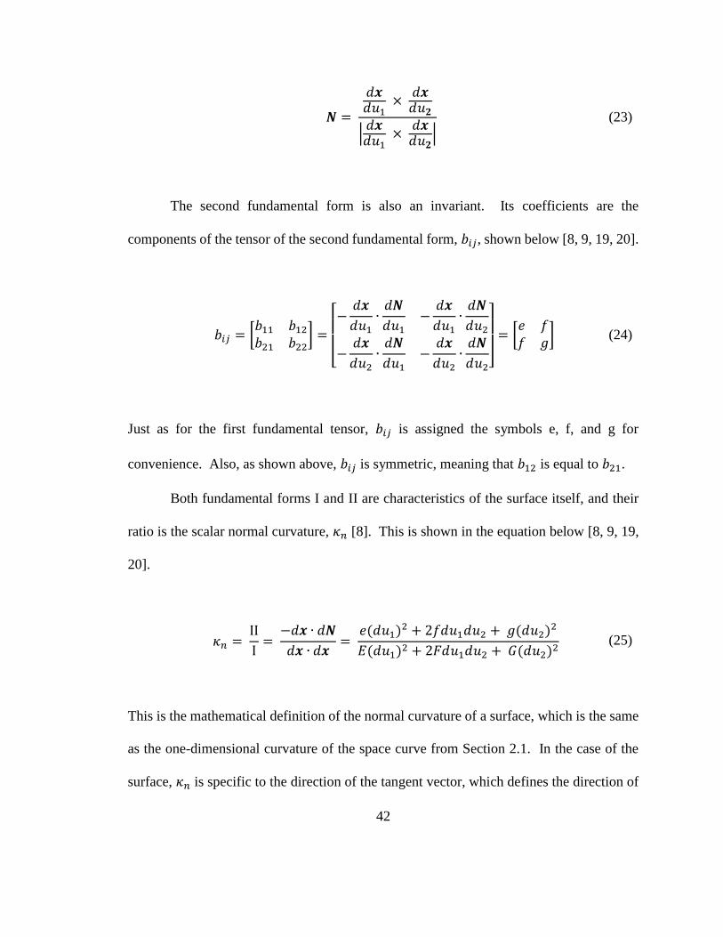
The second fundamental form is also an invariant. Its coefficients are the

components of the tensor of the second fundamental form, 𝑏𝑖𝑗, shown below [8, 9, 19, 20].

𝑏𝑖𝑗 = [𝑏11 𝑏12

𝑏21 𝑏22] =

[ −

𝑑𝒙

𝑑𝑢1∙𝑑𝑵

𝑑𝑢1−

𝑑𝒙

𝑑𝑢1∙𝑑𝑵

𝑑𝑢2

−𝑑𝒙

𝑑𝑢2∙𝑑𝑵

𝑑𝑢1−

𝑑𝒙

𝑑𝑢2∙𝑑𝑵

𝑑𝑢2]

= [𝑒 𝑓𝑓 𝑔

] (24)

Just as for the first fundamental tensor, 𝑏𝑖𝑗 is assigned the symbols e, f, and g for

convenience. Also, as shown above, 𝑏𝑖𝑗 is symmetric, meaning that 𝑏12 is equal to 𝑏21.

Both fundamental forms I and II are characteristics of the surface itself, and their

ratio is the scalar normal curvature, 𝜅𝑛 [8]. This is shown in the equation below [8, 9, 19,

20].

𝜅𝑛 =

II

I=

−𝑑𝒙 ∙ 𝑑𝑵

𝑑𝒙 ∙ 𝑑𝒙=

𝑒(𝑑𝑢1)2 + 2𝑓𝑑𝑢1𝑑𝑢2 + 𝑔(𝑑𝑢2)

2

𝐸(𝑑𝑢1)2 + 2𝐹𝑑𝑢1𝑑𝑢2 + 𝐺(𝑑𝑢2)2 (25)

This is the mathematical definition of the normal curvature of a surface, which is the same

as the one-dimensional curvature of the space curve from Section 2.1. In the case of the

surface, 𝜅𝑛 is specific to the direction of the tangent vector, which defines the direction of

43

the curve, and incorporates the second derivative of position with respect to movement

along the surface. For any point on S, there are an infinite number of curve directions and

associated curvatures. To find the normal curvature for any given tangent vector, the

Weingarten Equations must be used [19]. These equations use the two fundamental forms

to construct a third tensor 𝜅𝑖𝑗 which describes the complete state of curvature for a point

on a surface. This tensor is often called the Shape Operator, but can also be referred to as

the Weingarten Map or the tensor of curvature. The Weingarten Equations, and the

associated Weingarten tensor are given below [19, 20].

𝜅11 =

𝑓𝐹 − 𝑒𝐺

𝐸𝐺 − 𝐹2 (26)

𝜅12 =

𝑔𝐹 − 𝑓𝐺

𝐸𝐺 − 𝐹2 (27)

𝜅21 =

𝑒𝐹 − 𝑓𝐸

𝐸𝐺 − 𝐹2 (28)

𝜅22 =

𝑓𝐹 − 𝑔𝐸

𝐸𝐺 − 𝐹2 (29)

𝜅𝑖𝑗 = [𝜅11 𝜅12

𝜅21 𝜅22] (30)

In the case of orthogonal surface coordinates 𝑢1 and 𝑢2, the above tensor is symmetric so

that 𝜅12 = 𝜅21 [19]. It is the 𝜅𝑖𝑗 entities which are readily measurable by a localized sensor

array, which is the motivation for this particular investigation.

This tensor of curvature can define the curvature of a surface at a point based on a

chosen tangent vector. The maximum and minimum curvatures are given by the

44

eigenvalues of 𝜅𝑖𝑗, and are called the principal curvatures. These are denoted as 𝜅1 and 𝜅2,

and their corresponding eigenvectors 𝒗1 and 𝒗2 are known as the principal curvature

directions [8, 9, 19, 20]. These principal curvatures define the geometry of the surface for

which they are found. For this reason, they are extremely important to the goal of shape

sensing. By measuring the curvature in three different directions simultaneously, one can

construct the shape operator for a surface and thus find the principal curvatures.

Additionally, the tensor of curvature can potentially be used to find the fundamental forms

of a surface and establish a metric by which to measure said surface.

Other definitions for the curvature of a surface exist, but these typically incorporate

the principal curvatures. For instance, the Gaussian curvature 𝐾 is defined as follows [8]:

𝐾 = 𝜅1𝜅2 =

𝑏

ℊ (31)

The terms 𝑏 and ℊ are the determinants of the tensors 𝑏𝑖𝑗 and ℊ𝑖𝑗, respectively. The

Gaussian curvature is useful for classifying the type of surface geometry present, as its sign

changes depending on the signs of 𝜅1 and 𝜅2. Another commonly used expression is the

mean curvature 𝐻, which is defined below.

𝐻 =

1

2(𝜅1 + 𝜅2) (32)

45

The mean curvature is simply the arithmetic mean of the two principal curvatures. It quite

literally gives an average value for the curvature of a surface at a point. Like the Gaussian

curvature, the mean curvature can be positive, negative, or zero, depending on the surface.

This is because different surface geometries have differing principal curvatures.

𝜅1 and 𝜅2 can be positive or negative, and their associated directions are almost

always perpendicular to each other. The following figure shows several surfaces and their

principal curvature directions (Figure 13).

Figure 13: Principal Curvature Examples [21]

In each of the above cases, the point for which the principal curvatures are shown is the

intersection of the red and black lines. The black line follows the direction of the minimum

curvature, and the red line depicts the maximum curvature. For the object on the far left,

both principal curvature values are positive. The remaining two surfaces each have a

minimum curvature which is negative, assuming the convention in which the surface

normal extends outward from the surface and not into the surface. The signs of the

principal curvatures can be used to classify various surface geometries.

46

There are three possibilities regarding the signs of the principal curvatures of a

surface. The first is the case where both 𝜅1 and 𝜅2 have the same sign, such as on the first

body in (Figure 13). This point is called an elliptic point, and it can be identified as having

a dome-like geometry. Spheres exhibit a special case of elliptic geometry; because all

directions have equal curvature, all directions are principal curvature directions.

Additionally, all points on a sphere are umbilics, which are points on a surface for which

all directions contain principal curvatures. This is the only time that the directions

associated with 𝜅1 and 𝜅2 are not necessarily perpendicular, as every direction is a principal

curvature direction. For any elliptic point, the Gaussian curvature 𝐾 is always positive.

This is true for both convex and concave surfaces, as the principal curvatures will always

have the same sign, regardless of convention.

The next type of surface geometry is called a parabolic point. These are points at

which one of the principal curvatures is equal to zero. Technically, there is an additional

geometry classification for which both 𝜅1 and 𝜅2 are zero. This is trivially a plane, for

which the expected curvature would always be zero. As discussed in Section 2.3.1, a

simple example of a parabolic surface is the side of a cylinder, which experiences no

curvature in the longitudinal direction. Parabolic points are characterized by a nonexistent

Gaussian curvature; when either 𝜅1 or 𝜅2 is zero, then so is the product of these two

principal curvatures.

The final classification of surface geometry is a hyperbolic point, which is

characterized by two nonzero principal curvatures of opposite sign. The saddle geometry

in (Figure 12) and the remaining two surfaces in (Figure 13) portray this type of geometry.

47

The Gaussian curvature of a hyperbolic point will always be negative due to the sign

difference in 𝜅1 and 𝜅2. Saddle curves are of particular interest to this study, as the two

opposing curvatures are not easily captured by contemporary sensing methods. Using

either FBGs or flex sensors in their contemporary configurations, only one principal

curvature could be measured, leaving much of the surface unknown. This is of course

assuming that the sensors are intentionally aligned with the principal curvature directions.

If the sensors were placed such that the curvature in a non-principal direction was

measured, the resulting measurement would be less useful for determining the surface

geometry. This is true for any of the three geometry classifications listed here, but

especially for the hyperbolic point.

In order to determine the shape of a surface, the curvature must be measured in

more than one direction. It is particularly useful to measure the curvature in known

directions of principal curvature. If the principal curvature values are known, then the

shape of the surface can be determined. By starting with the principal curvatures and

essentially working backwards, the underlying geometry of the surface could be inferred.

This is not unlike the method employed by the NASA FBG chain effort discussed in

Section 2.2.1. However, successful shape determination of a two-dimensional surface

requires curvature measurements to be taken in multiple directions simultaneously. This

in turn requires a novel sensor array, which was developed as the second major task in this

investigation. The design, fabrication, and testing of this new surface curvature sensor are

discussed at length in the next section.

48

3.2. Sensing Curvature in Multiple Directions

3.2.1. Design Objectives and Theory

The purpose of the proposed sensor array is to capture the curvature of a surface.

The objective of this design was then to measure curvature in multiple directions at one

time. Specifically, this array was designed with two sensors that could take curvature

readings in two separate, orthogonal directions. These would be aligned with the principal

curvature directions of a test surface in order to ascertain the geometry thereof.

Additionally, the curvature in the direction between the two principal directions would be

measured by a third sensor. This would help to bridge the gap between the two principal

curvatures and shed additional light on the geometry of the surface. This sensor

configuration is consistent with that of a strain-sensing rosette, the measurements from

which can be used to construct the strain tensor. The rosette layout was chosen for this

application in order to take the measurements necessary to construct the metric tensor for

a surface. From this, along with the principal curvatures, the fundamental forms could be

derived and the shape of the surface defined. Because the rosette configuration was

implemented in its design, this novel sensor array will be referred to as the Curvature-

Sensing Rosette (CSR).

Once the basic concept of the CSR was formulated, the specific method of

curvature detection was chosen. In light of the limitations of the CBIC due to the

inaccuracy of its flex sensors, the FBG method was selected for use in the CSR. As stated

previously, this method requires two FBGs separated by a known distance in order to

measure curvature. The CSR was designed to be a patch of known thickness with three

49

FBGs attached to either side of it. This patch could either be affixed to the surface of an

inflatable, or the sensor configuration could be embedded in the inflatable material itself.

The six FBGs form three separate pairs, each capable of sensing curvature in a single

direction. The CSR would then be able to measure curvature with a high level of accuracy

in three different directions simultaneously. The FBG pairs would also eliminate additional

strain due to stretching, as this behavior on one side would get cancelled out by the other.

In order to test the accuracy of the CSR, a test surface of known geometry is used.

A surface with hyperbolic geometry was chosen for testing, as it could best demonstrate

the utility of the CSR. In order to be defined, the opposite principal curvatures of the saddle

surface would require a sensor which could detect curvature in multiple directions.

Provided the shape of the saddle surface could be detected, the CSR could be tested on

various other geometries.

Ideally, the CSR could be applied to any surface without prior knowledge of the

geometry. Recall that the surface, metric, and Weingarten tensor are all defined with

respect to a pair of orthogonal coordinates, 𝑢1 and 𝑢2. If the directions of 𝑢1 and 𝑢2 are

aligned with the principal curvature directions, then the tensor of curvature simplifies to a

diagonal matrix comprised of the principal curvatures, as shown below.

𝜅𝑖𝑗 = [

𝜅11 𝜅12

𝜅21 𝜅22] = [

𝜅1 00 𝜅2

] (33)

As it stands, the two orthogonal sensor pairs are intended to align with the principal

curvatures. However, assuming enough information can be gathered by the CSR about the

50

surface geometry, then the direction of the principal curvatures need not be known. The

Weingarten tensor of curvature could be constructed by performing a coordinate

transformation on the measurements taken by the CSR.

Consider a single pair of orthogonal coordinates 𝑢1 and 𝑢2, with directions 𝒆1 and

𝒆2, respectively. Rotated an angle 𝜃 about the origin is a new set of orthogonal coordinates,

𝑢1′ and 𝑢2

′, with directions 𝒆1′ and 𝒆2

′, respectively. This is illustrated in the figure below

(Figure 14).

Figure 14: Rotation of Coordinate Axes

In some cases, it may be convenient to establish a new set of coordinates which simplify

calculations. In order to transform the original coordinates into the new prime coordinates,

the direction cosine matrix is used. This matrix gives a mapping from the original

coordinates to the new set, and is based on the angle between the two coordinate systems.

This transformation matrix is shown below.

51

𝑎𝑖𝑗 = [

𝒆1′ ∙ 𝒆1 𝒆1

′ ∙ 𝒆2

𝒆2′ ∙ 𝒆1 𝒆2

′ ∙ 𝒆2] = [

𝑐𝑜𝑠𝜃 𝑠𝑖𝑛𝜃−𝑠𝑖𝑛𝜃 𝑐𝑜𝑠𝜃

] (34)

Recall that the curvature tensor is formulated using the two fundamental forms, which are

invariants. This means that the curvature tensor is also an invariant and thus does not

change even as the coordinate system does. So, the curvature tensor 𝜅𝑖𝑗 can be transformed

into 𝜅𝑖𝑗′ using the following equation, without affecting the tensor itself.

[𝜅𝑖𝑗′] = [𝑎𝑖𝑗]

𝑇 [𝜅𝑖𝑗] [𝑎𝑖𝑗] (35)

In the above equation, the superscript ‘T ’ denotes a transposed matrix. With this equation,

the curvature measurements from the CSR can be transformed into another coordinate

system, such as the principal coordinates. These are the set of axes which are aligned with

the principal directions.

In order to obtain 𝜅𝑖𝑗 from three arbitrary curvature measurements, one must utilize

an inherent property of the Weingarten Map, which gives a value of normal curvature for

any specified tangent direction [19, 20]. Suppose a curvature sensing rosette was placed

on a surface with parameters 𝑢1 and 𝑢2. The following figure illustrates this (Figure 15).

52

Figure 15: CSR on Coordinate Axes

Note that the three blue rectangles show where the curvature sensing FBG pairs would be.

These FBG pairs give curvature readings of 𝜅(0°), 𝜅(45°), and 𝜅(90°) as shown. By

choosing an arbitrary coordinate system aligned with the direction of 𝜅(0°), we can write

the following [19, 20].

𝜅(0°) = 𝒆1 ∙ 𝜅𝑖𝑗 ∙ 𝒆1 (36)

𝜅(0°) = [1 0] [𝜅11 𝜅12

𝜅21 𝜅22] [

10] = 𝜅11 (37)

Note that equations (36) and (37) are equivalent, because [10] is the coordinate

representation of the unit vector 𝒆1. By aligning the surface coordinate axes with the first

FBG pair, the first term in the curvature tensor is instantly found. Similarly, the 𝜅22 term

can be found with the following expressions.

53

𝜅(90°) = 𝒆2 ∙ 𝜅𝑖𝑗 ∙ 𝒆2 (38)

𝜅(90°) = [0 1] [𝜅11 𝜅12

𝜅21 𝜅22] [

01] = 𝜅22 (39)

Again, this is the utility of the Weingarten curvature tensor. In order to find the final

component, the vector in the direction of the central FBG pair must be used.

𝜅(45°) = (

√2

2𝒆1 +

√2

2𝒆2) ∙ 𝜅𝑖𝑗 ∙ (

√2

2𝒆1 +

√2

2𝒆2) (40)

𝜅(45°) =1

2[1 1] [

𝜅11 𝜅12

𝜅21 𝜅22] [

11] (41)

𝜅(45°) =

1

2[𝜅11 + 2𝜅12 + 𝜅22] (42)

Equation (42) can be written as such because the curvature tensor is symmetric for all

orthogonal coordinate systems, so 𝜅12 = 𝜅21. Now the known values for 𝜅11 and 𝜅22 can

be substituted into equation (42), and the final component of the curvature tensor can be

found.

With the Weingarten curvature tensor known, the principal curvatures and their

directions can be found. With these directions known, the local area surrounding the CSR

could be defined. By placing multiple CSRs about an inflatable, the overall shape can be

determined. This is the intended long-term use for the CSR. The scope of this project,

however, only included testing of the CSR on a controlled test surface.

54

3.2.2. Fabrication and Testing

This section details the process by which the proposed CSR was produced and

subsequently tested. As a preliminary experiment, a single FBG pair was constructed and

its accuracy tested. A sample specimen was affixed with an FBG (FBGS SG-01) on either

side. This specimen was clamped to a wooden test block of known curvature. The FBGs

were connected to an Optical Sensor Interrogator (OSI) (National Instruments PXIe-4844),

which performed the action of sending a spectrum of white light down the two fibers and

recording their respective reflected peaks. With data acquisition software capturing the

FBG behavior, the test specimen was bent from an initially straight position to match the

curve of the wooden block. This experimental setup can be seen in the figure below (Figure

16).

Figure 16: FBG Bend Test Setup

The process of bending the specimen to the wooden block, then back to true was repeated

several times. The data collected from the test are shown in the following graph (Figure

17).

55

Figure 17: Bend Test Data

In the graph above, the vertical axis shows the wavelength of the reflected peaks of each

of the FBGs throughout the test. The horizontal axis is arbitrary time; as none of the

primary results are time-dependent, the units were omitted. Note that the order of the two

data series on the graph is merely a result of the wavelengths of the reflected peaks of each

FBG. The legend shows which data series corresponds to each sensor channel. In this

case, the orange data were collected from the FBG in compression, or the FBG on the

bottom of the test specimen in (Figure 16). This means that the blue data corresponds to

the FBG on the top in (Figure 16), which would be in tension during the bending portion

of the test. This is easily seen in the behavior of the data sets. A peak in the lower line on

the graph corresponds to a fully bent specimen, which would result in the maximum tension

being applied to the FBG on the top in (Figure 16). This occurs during a trough in the

upper line on the graph, which corresponds to the maximum compression of the FBG on

the bottom in (Figure 16). As previously stated, the test specimen was bent, then

1528

1529

1530

1531

1532

1533

1534

1535

1536

1537

1538

Ref

lect

ed W

avel

ength

(nm

)

FBG Bend Test

Dev0/Ch0/Sen0

Dev0/Ch1/Sen0

56

straightened, then bent again. From the graph, it can be seen that this procedure was

performed a total of three times before the test was concluded. The values of the

wavelengths of the reflected peaks before and after one such bending procedure, as well as

the calculated strain, are tabulated below (Table 1).

Table 1: FBG Bend Test Data

Sensor Channel 𝝀𝒐 (nm) 𝝀 (nm) 𝜺

0 1529.526 1530.668 0.000934

1 1537.245 1537.053 -0.000157

The values for 𝜆𝑜were chosen from the first flat portion of the graph, before the specimen

was subjected to bending. The 𝜆 values were taken from a time corresponding to a peak in

the lower data series. This represents the time when the maximum bending, and thus

curvature, occurred. Using the FBG equation (9) found in Section 2.2.1 and ignoring the

effects of temperature, the strain 𝜀 in each FBG was calculated from the measured

wavelength shift. Note that these particular FBGs had a gauge factor of 0.799, as opposed

to the standard value of 0.78. This was provided by the manufacturer and had no impact

on the outcome of the test. By taking the difference in strain ∆𝜀 between the top and bottom

FBGs, and then dividing through by the thickness of the test specimen, an experimental

value for the curvature was obtained. The results of this initial test are shown in the

following table (Table 2).

Table 2: FBG Bend Test Results

∆𝜺 𝜿𝒆𝒙𝒑 (𝐦𝐦−𝟏) 𝜿𝒂𝒄𝒕 (𝐦𝐦−𝟏) Accuracy (%)

0.0010904 0.002647 0.002625 99.17

57

The value for the true or actual curvature 𝜅𝑎𝑐𝑡 was found by taking the inverse of the known

radius of the wooden block, which was 381 mm (15 inches), the inverse of which is

0.002625 mm-1. As shown in the table, the accuracy of this method was found to be

99.17%, meaning that the experimental value for curvature was within one percent of the

actual value. This level of accuracy is expected of FBGs. In fact, minor inaccuracies of

the wooden test block could just as easily be responsible for the less than one percent

discrepancy as the FBGs. In any case, the accuracy of the FBG method of sensing

curvature was deemed acceptable for the CSR.

In order to successfully fabricate the CSR as designed, the above process would

need to be repeated three-fold. This would require a total of six FBGs, which exceeds the

number of available ports on the OSI by two. A multiplexed FBG chain was used to

circumvent this issue. This custom-ordered multiplexed fiber was comprised of sixteen

FBGs, each of which had a unique wavelength for its reflected peak. These wavelengths

varied from 1,510 to 1,590 nm, as this was the operating range of the OSI. The wavelength

values of the FBGs progressed in order with increasing distance along the length of the

fiber. Thus, the location of each FBG in the multiplexed chain could be determined by its

wavelength.

The rosette design was measured out and drawn on the surface of the intended

material for the CSR. A vinyl patch from a swimming pool repair kit was chosen for its

flexibility and resilience to tearing. The multiplexed fiber was looped around the rosette

design so that all six necessary FBGs could be aligned with their respective axes. The

alignment of the FBGs in the CSR can be seen in the following figure (Figure 18).

58

Figure 18: Curvature Sensing Rosette

The three straight lines in the image above are the three directions along which the

curvature will be measured. The clear fiber can be seen looping about these lines, ensuring

that each FBG is positioned correctly. A thin slit was cut in the vinyl to allow the fiber to

pass from one side of the patch to the other, so that three of the FBGs could be attached to

the back side. The location of each FBG in the fiber is labeled with two black tick marks

separated by approximately 1.5 inches; the FBG is located in between these marks. By

securing the tick marks to the specified axes, the FBGs were guaranteed to lie on said axes.

Several adhesives were tested for this application, based on recommendations made in [22].

59

In the end, cyanoacrylate adhesive was used to secure the fiber to either side of the vinyl

patch along the drawn lines. Pressure sensitive tape (Kapton) was used to secure the fiber

beyond the glued portion in order to protect the fragile loops from potential damage. The

fabrication of the prototype CSR was thus completed and ready for testing.

While the construction of the CSR was relatively straightforward, the subsequent

testing proved to be far more problematic. Finding a suitable saddle surface with which to

calibrate the CSR was much more difficult than anticipated. It is true that saddles exist as

a part of several common geometries, such as a torus. However, actually finding a saddle

whose geometry could be quantified for testing purposes was a challenge. It was originally

proposed that a section of an inflatable torus be outfitted with the sensor throughout a full

inflation procedure. This would only serve as a qualitative test, as the only way to quantify

the curvature of the saddle during inflation would be to employ the exact type of sensor

being tested.

Moreover, initial testing showed that the CSR would not be usable on many

available surfaces. This is due to the nature of the multiplexed FBG chain and the OSI to

which it is connected. When the FBG chain is connected to this OSI, the sixteen reflected

peaks are easily detected by the software. In the configuration window, one can set specific

ranges in which a peak of interest, such as the six peaks that comprise the CSR, might be

found. An example of this window is shown in the figure below (Figure 19).

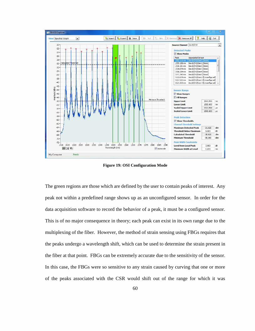
60

Figure 19: OSI Configuration Mode

The green regions are those which are defined by the user to contain peaks of interest. Any

peak not within a predefined range shows up as an unconfigured sensor. In order for the

data acquisition software to record the behavior of a peak, it must be a configured sensor.

This is of no major consequence in theory; each peak can exist in its own range due to the

multiplexing of the fiber. However, the method of strain sensing using FBGs requires that

the peaks undergo a wavelength shift, which can be used to determine the strain present in

the fiber at that point. FBGs can be extremely accurate due to the sensitivity of the sensor.

In this case, the FBGs were so sensitive to any strain caused by curving that one or more

of the peaks associated with the CSR would shift out of the range for which it was

61

configured. This immediately causes the peak(s) in question to become unconfigured,

meaning they cannot be measured by the software. There are a few means of solving this

problem, but most of these require an entirely new multiplexed FBG chain to be used in

place of the current one. This was not a viable option for a number of reasons. There was,

however, a solution which could also solve the problem of finding a suitable test surface.

The proposed solution involved the designing of a test surface using CAD software,

which could then be 3-D printed for experimentation. In this way, an ideal saddle surface

could not only be produced, but the exact principal curvatures would be defined in the CAD

software. More importantly, the curvature of the test surface could be deliberately set to a

very low value. This would ensure that the wavelength shift would be minimal, yet still

measureable for FBGs. The issue regarding the unconfigured sensor peaks was only a

problem for most surfaces because the amount of curvature present on those surfaces was

enough to cause the peaks to shift out of their predefined ranges. However, by defining

low principal curvature values, the measured peaks would be able to shift a detectable

amount without shifting beyond their allowed range. Additionally, from a theoretical

standpoint, detecting a very shallow curve would demonstrate the accuracy of the CSR

much better than would a severe curve.

Using the CAD program Solidworks, the test saddle surface was designed. This

geometry was achieved by revolving the two-dimensional profile of a circle about another

circle which lay in a plane perpendicular to the first. This produced a virtual torus, the

inner surface of which exhibits saddle geometry. The majority of the torus was then ‘cut’

away, leaving a small section with saddle geometry. The radii of the original two circles

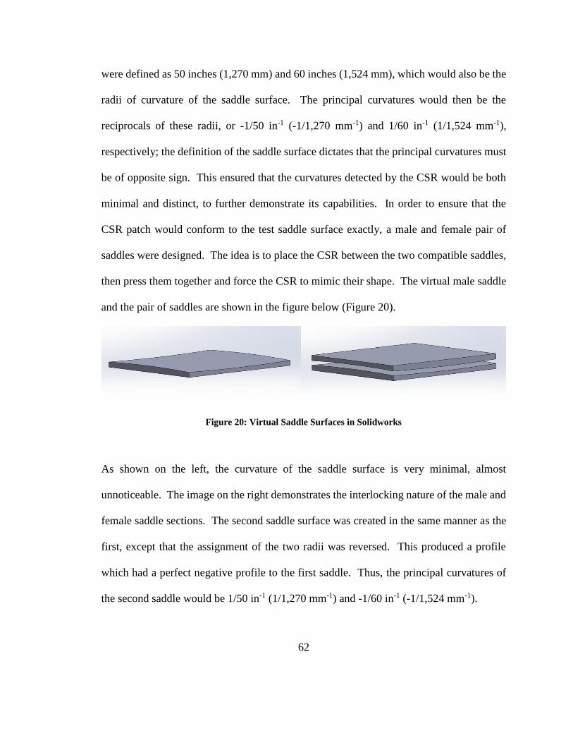
62

were defined as 50 inches (1,270 mm) and 60 inches (1,524 mm), which would also be the

radii of curvature of the saddle surface. The principal curvatures would then be the

reciprocals of these radii, or -1/50 in-1 (-1/1,270 mm-1) and 1/60 in-1 (1/1,524 mm-1),

respectively; the definition of the saddle surface dictates that the principal curvatures must

be of opposite sign. This ensured that the curvatures detected by the CSR would be both

minimal and distinct, to further demonstrate its capabilities. In order to ensure that the

CSR patch would conform to the test saddle surface exactly, a male and female pair of

saddles were designed. The idea is to place the CSR between the two compatible saddles,

then press them together and force the CSR to mimic their shape. The virtual male saddle

and the pair of saddles are shown in the figure below (Figure 20).

Figure 20: Virtual Saddle Surfaces in Solidworks

As shown on the left, the curvature of the saddle surface is very minimal, almost

unnoticeable. The image on the right demonstrates the interlocking nature of the male and

female saddle sections. The second saddle surface was created in the same manner as the

first, except that the assignment of the two radii was reversed. This produced a profile

which had a perfect negative profile to the first saddle. Thus, the principal curvatures of

the second saddle would be 1/50 in-1 (1/1,270 mm-1) and -1/60 in-1 (-1/1,524 mm-1).

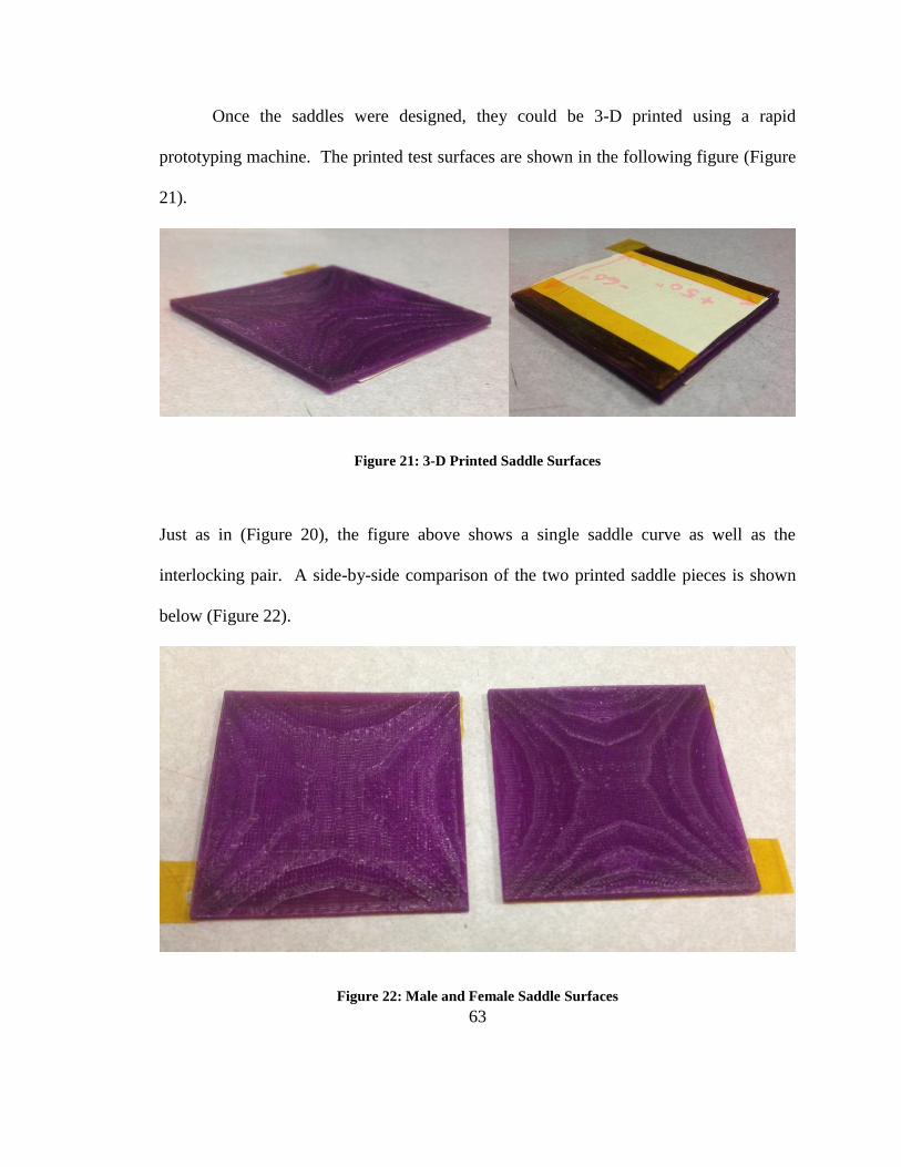
63

Once the saddles were designed, they could be 3-D printed using a rapid

prototyping machine. The printed test surfaces are shown in the following figure (Figure

21).

Figure 21: 3-D Printed Saddle Surfaces

Just as in (Figure 20), the figure above shows a single saddle curve as well as the

interlocking pair. A side-by-side comparison of the two printed saddle pieces is shown

below (Figure 22).

Figure 22: Male and Female Saddle Surfaces

64

The lines on the two surfaces above are characteristic of the fused deposition modeling

(FDM) style of 3-D printing. The printed part is essentially built in layers, meaning that

the continuous curves in the virtual design will be printed out as discretized sections which

attempt to approximate a curve. The implications of this will be further explored in Section

3.2.3.

With the saddles printed, the testing of the CSR could begin. The rosette was

initially placed on a flat surface and pressed down with the acquisition software running so

that an initial wavelength could be found for each reflected peak which corresponded to

the absence of curvature. Then the CSR was placed on the male test saddle surface, as

shown below (Figure 23).

Figure 23: The CSR on the Male Test Saddle

65

Note that the two perpendicular axes of the CSR have been aligned with the principal

curvature directions of the test saddle. The third direction runs straight through the center

of the saddle, in which direction the expected curvature would be extremely minimal.

Next, the female saddle piece was placed on the CSR and carefully aligned to the male

saddle surface. This was done using tabs of Kapton tape that had been applied to the printed

saddle pieces for exactly this reason. The following figure shows the CSR between the

two saddles (Figure 24).

Figure 24: CSR and Saddle Pair Assembly

The top saddle piece was then pressed downwards in order to force the CSR patch to

conform to the shape of the two saddles. The entire CSR and saddle pair assembly was

66

pressed down and subsequently released several times during the test. The figure below

shows the window of the data acquisition software during this time (Figure 25).

Figure 25: Data Acquisition for the CSR Test

The data were then saved for subsequent analysis. The results of the preceding test are

presented in the next section.

3.3.3. Results and Discussion

The CSR test data were analyzed in the same manner as the initial bending test,

except of course that two additional curvatures were calculated. From a qualitative

standpoint, the test was a complete success; the three curvatures measured by the CSR are

all of the appropriate sign and order of magnitude. However, the extremely high accuracy

67

of the single FBG bend test was not present in the CSR test. There are a number of factors

that likely contributed to this inaccuracy, and many of these can be overcome.

The data acquired in (Figure 25) were inspected for usable measurements. Despite

the efforts made to ensure that all six of the sensors remained configured throughout the

test, there were still some instances in which one or more sensors’ data were not collected.

This is due in part to the aforementioned issue of configured sensors, but also due to the

occasional presence of multiple peaks. The single peak of an FBG can become noisy after

encountering too many tight bends in the fiber optic cable. This is because a tight bend

essentially increases the angle of internal reflection required for a light signal to remain

within the fiber. This can cause the original light to be dispersed as a portion of it escapes

the fiber or gets scattered. This results in the presence of multiple peaks showing up within

the predefined range of a single peak, which causes the sensor within that range to be in a

so-called error state. Just as when a sensor is unconfigured, this results in no data being

collected for a sensor while it is in a state of error.

Out of the several instances when the saddle assembly was pressed to give the CSR

the same shape as the saddles, only one trial yielded measured values for all six sensors.

The following figure shows a graph of this successful trial, and an example of a trial which

was ultimately not used due to one or more sensors being in error state (Figure 26).

68

Figure 26: Sample Data from the CSR Saddle Test

Note how on the far left, all sensors are present and apparently reading constant curvature.

This corresponds to the time when the CSR was initially pressed into a flat configuration.

Moving to the right, there is a point at which the top-most sensor disappears from the graph.

This is actually during the process of removing the CSR from the flat surface and onto the

male saddle piece. The CSR patch was unintentionally bent through a relatively extreme

curve during this transition. The missing sensor, which has the highest wavelength, is the

sensor which is furthest from the interrogating light source. This light must therefore pass

through the most loops before reaching this FBG, which is why this sensor is shown to be

in error state. Once the CSR is placed in the saddle assembly, the missing sensor returns

and all six FBGs seem to level off. That is until the saddle pieces are pressed together for

a time, then released once more. This describes the phenomenon to the left of the graph.

Note how some sensors show a positive shift, while others indicate a negative shift in

wavelength. Just as with the simple bend test, the positive values correspond to the FBGs

1550

1555

1560

1565

1570

1575

Ref

lect

ed W

avel

ength

(nm

)

CSR Saddle Surface Test

Dev0/Ch0/Sen0

Dev0/Ch0/Sen1

Dev0/Ch0/Sen2

Dev0/Ch0/Sen3

Dev0/Ch0/Sen4

Dev0/Ch0/Sen5

69

in tension whereas the negative shifts correspond to FBGs in compression. Once more,

their measured peak values, as well as their calculated strains, are tabulated below (Table

3).

Table 3: CSR Saddle Test Data

Sensor 𝝀𝒐 (nm) 𝝀 (nm) 𝜺

0 1552.149 1551.726 -0.000349

1 1555.355 1555.500 0.000120

2 1559.830 1560.649 0.000673

3 1564.356 1564.744 0.000318

4 1567.842 1567.815 -0.000022

5 1571.776 1571.354 -0.000344

As expected, three of the calculated strains are positive and three are negative. Due to the

layout of the FBG pairs, and immediate qualitative understanding of the surface can be

inferred. Refer to the following schematic diagram of the CSR for clarification (Figure

27).

70

Figure 27: CSR Schematic Diagram

Note that the blue section of the fiber represents the portion on the top of the patch material;

the red represents the portion on the bottom. The thicker rectangular objects represent the

FBGs. The location of the slit in the patch material is labeled. This is where the fiber

passes through the material. Notice that the pairs are as follows: sensors 0 and 3, sensors

1 and 4, and sensors 2 and 5. The three sensors numbered from 0 to 2 are on the top of the

patch, and the sensors numbered from 3 to 5 are on the bottom. By looking at the strain

values in Table 3, it can be seen that the curvature is negative in the direction aligned with

sensor 0, which is a principal curvature direction, and positive for the other two directions.

71

This is a simple qualitative check of the CSR, and it is consistent with the expected saddle

geometry. The quantitative results are listed in the table below (Table 4).

Table 4: CSR Saddle Test Results

Sensor Pair ∆𝜺 𝜿𝒆𝒙𝒑 (𝐦𝐦−𝟏) 𝜿𝒂𝒄𝒕 (𝐦𝐦−𝟏) Accuracy (%)

0 and 3 -0.000667 -0.001876 -0.000656 34.96

1 and 4 0.000142 0.000398 0.000066 16.48

2 and 5 0.001017 0.002861 0.000787 27.52

First, it should be noted that the FBG pair consisting of sensors 1 and 4 was directed

between the principal curvature directions. Using the theoretical eigenvalues for the two

principal curvatures, the 𝜅𝑎𝑐𝑡 table entry for the central FBG pair was calculated. The fact

that the measured curvature is far less than that of the principal directions is again

consistent with the saddle geometry of the test surface. For the other two pairs, which align

with the principal directions, the sign and relative magnitudes of the measured curvatures

are also fairly consistent. However, the accuracy of each measured curvature when

compared to its true or actual value is far from ideal. Given that they were all much smaller

than expected, it was believed that the separation distance between the sensors was in fact

greater than originally thought.

Recall again the equation (10) from Section 2.2.1 which gives a curvature reading

based on two FBG strain sensors. The difference in strain is divided by the separation

distance, which in this case was the thickness of the patch material. Although the thickness

of a sample portion of the patch material was measured prior to the construction of the

CSR, it is likely that the final thickness of the material between the sensor pairs differed

72

from the initial measurement. Not only is the patch itself likely to vary in thickness due to

manufacturing tolerances, but any amount of excess adhesive could build up and contribute

to the overall thickness. To put this in perspective, the initial thickness of the patch was

measured via optical comparator and found to be 356 μm. This is barely larger than a third

of a millimeter. If a similar thickness of adhesive was deposited on each side of the patch,

then the total patch thickness would increase by a factor of three. This is roughly the factor

by which the measured principal curvatures differ from their expected actual values.

Given that the accuracy of this FBG curvatures sensing method was demonstrated

during the simpler bend test, this unknown thickness increase is likely the cause of the

inaccuracy of the CSR test results. It should be noted that the bend test results were not

affected in the same manner because the thickness of the test specimen itself was several

orders of magnitude greater than the supposed added thickness of the adhesive. For the

CSR Saddle test, the fact that the values of the inaccuracies of the principal curvatures vary

between themselves would indicate that the unknown combined thickness of the patch and

adhesive is itself variable. The fact that the central FBG pair shows the greatest

discrepancy is likely due to a combined error due to unknown separation distance and test

surface quality. The characteristic layers of the FDM rapid prototyping process can be

plainly seen in (Figure 22). Because this direction theoretically had the least amount of

curvature by an order of magnitude, any surface inconsistencies would be greatly reflected

by the overall accuracy of this FBG pair.

Assuming that the FBG method itself was accurate, the actual curvature values were

used to solve for the true separation distances, thereby attempting to calibrate the CSR.

73

The new thickness of the materials between sensors 0 and 3 was found to have increased

by a factor of 2.86, while the thickness between sensors 2 and 5 had increased by a factor

of 3.63. These resulted in thicknesses of 1.0 mm and 1.3 mm, respectively. Again, this

seems to be a plausible thickness for both patch material and adhesive. The central FBG

separation distance was calibrated to be 2.16 mm; however, this may or may not be accurate

depending on the error in the test surface in this direction.

The apparent variability of the true thickness of the material between sensor pairs

make for a difficult summary of the overall accuracy of the CSR. Any statement regarding

its accuracy would necessarily be made with caveats. That being said, the success of the

Saddle test from a qualitative standpoint does indicate that the CSR has the potential to be

more accurate, provided some adjustments are made. These are necessary improvements

for making the CSR a viable option for measuring the curvature of a surface. Once

implemented, these alterations could make the CSR the preferred curvature sensor for next-

generation inflatable shape sensing systems.

First and foremost, the issue of the excess deposition of the cyanoacrylate adhesive

must be addressed. This is the main cause of the inaccuracy of the CSR, and solving this

issue would likely remove the need for calibrating the CSR in the directions of principal

curvature. Fortunately, there are several methods listed in [22] which can improve the

consistency with which the adhesive is applied. One such method involves using a glass

form to hold the fiber in place while gluing it to the patch material. Another technique

requires the use of Kapton tape to secure the FBG while a low-viscosity adhesive is

vacuum-pumped along the length of the fiber. This allows the adhesive to fill any gaps

74

between the Kapton and the patch material [22]. Finally, a number of thermoplastic resins

could be used in place of the cyanoacrylate adhesive. These would require forms to be

placed over the FBGs while the resin is poured and cured. In general, any deliberate

method for attaching the fiber to the patch material in a consistent manner could be utilized

with great effect.

The next major area for improvement of the CSR is the configuration of the

multiplexed FBG chain which contains the important stain sensors. As stated, the

particular multiplexed fiber that was used in this investigation was less than ideal. This

was a result of nothing more than a learning curve associated with purchasing multiplexed

FBG chains. The specific fiber used here was ordered with the intent of obtaining a large

number of sensors in a single fiber. Because of the lead times associated with ordering a

custom multiplexed FBG chain, the final design of the CSR was not yet known at the time

of the purchase. The required functionality of the fiber chain was pure conjecture when it

was ordered. Had the CSR design been finalized, the FBG chain could have been made to

contain only six FBGs. For the same range of 1,510 to 1,590 nm, this would greatly

increase the separation of the wavelengths associated with each FBG. This means that

when configuring the software to detect each peak, a much wider range could be listed in

which to find said peak. This in turn would allow the CSR to remain functional over

surfaces with higher curvature magnitudes than the specially designed test surface.

Additionally, the physical spacing of the FBGs along the fiber could have been increased

significantly. This would mean that more fiber length could be used to make the same

turns that were necessary to align the FBG pairs with the predefined axes of curvature

75

measurement. The result would be a much greater bend radius of the fiber in between

FBGs, which would reduce the loss of signal and multiple peaks caused by excessive

bending in the fiber. Finally, six individual fibers could be used to produce the same FBG

layout required by the CSR. However, this would require a fiber bundle to reach the CSR

as opposed to a single fiber. This can potentially be quite arduous, considering the number

of CSRs that would likely be needed to sense the shape of a space inflatable. As it stands,

several CSRs could be made on a single multiplexed fiber, which would likely more useful

to any potential shape sensing system. Another alternative is to create a network of

multiplexed fibers to produce an array of CSRs, shown in the figure below (Figure 28).

Figure 28: Proposed CSR array

The configuration shown in the figure above could be implemented on an inflatable

surface, with three FBGs forming a CSR at each intersection.

The final area for improving the results of the CSR saddle test is in the making of

the test surface itself. While the virtual designs of the two saddle surfaces were ideal, the

physical printed part was flawed. This is due to the FDM style of rapid prototyping, which

deposits layers of molten plastic from a heated nozzle. This causes every piece printed this

76

way to have a surface texture, as well as discretized curves. There are several methods

described in [23, 24] which could greatly reduce these effects, making the saddle pieces

much smoother. Additionally, the resolution of the pieces could have been improved by

using a more precise machine. Of course, there is a higher cost associated with these high

resolution 3-d printers, and this would need to be considered. Employing either of these

strategies could reduce the texture of the test surface itself, thus improving the overall

accuracy of the test results.

Assuming that the above changes can be implemented, the accuracy of the CSR

could be dramatically improved. This would make it a viable option for sensing the surface

curvature of inflatable space structures, or any body for which the geometry must be

defined. This is because there are several features inherent to its design which allow the

CSR to be tailored for individual applications.

For example, the patch design allows for a simple surface application of the CSR,

but a more permanent embedding of the sensor array could be achieved with the same

sensor configuration. The patch material itself could be replaced with a more rigid or

flexible alternative, depending on the application.

Additionally, the layout of the FBGs could be customized for specific geometries.

In the current design, there is actually an offset of roughly one inch between the FBGs

themselves and the point at which their axes intersect. This was not an issue for the saddle

test, but may be for more irregular geometries. For an intricately detailed body, or a

particularly vital section of a body, the sensors could be spaced much more closely

together. Conversely, for a large or relatively simple body, the sensors could be spaced

77

more widely apart. This is true of the spacing of the CSR arrays as well. In fact, all of the

customizing options discussed for the bend sensors of the CBIC in Section 2.3.3 are

likewise applicable to the CSR. These qualities make the CSR a potentially viable solution

for the current need for accurate shape sensors.

78

CHAPTER 4: CONCLUSIONS

One of the many strides being made in the growing field of space exploration is the

use of inflatable structures. These inflatable bodies offer many advantages over traditional,

rigid structures, but present some unique challenges as well. Among these is the need for

accurate determination of the complete geometry of the body, known as shape sensing.

This is an important tool for monitoring both the inflation status and overall health of

inflatables. While differential geometry can describe the shape, it cannot be directly

measured. Instead, the surface curvature at certain point on a body is measured, and the

underlying geometry can be inferred.

This surface curvature exists in two dimensions, yet contemporary methods can

only measure one-dimensional curvature. This is the curvature which is characteristic of a

space curve, which is a one-dimensional mathematical construct. Although space curves

exist in three dimensions, they are subject to curvature in one and only one direction at a

time. This means that current techniques for sensing curvature only describe a single space

curve and not an entire surface. To circumvent this issue, NASA has developed a multi-

core, multiplexed chain of Fiber Bragg Gratings. This device is essentially a self-sensing

space curve, which can detect one-dimensional curvature in any direction. These curvature

measurements are used in subsequent calculations to produce a virtual image of the FBG

chain itself. By overlaying this fiber bundle on an unknown surface, the virtual image will

provide a limited depiction of said surface. Alternative methods are required to truly

identify the geometry of an unknown surface.

79

One such alternative is the flex sensor, which is a widely available and highly

economic option. However, in addition to being generally less accurate, these one-

dimensional curvature sensors suffer from similar pitfalls as the NASA FBG chain.

Despite this, their availability and ease of operation made flex sensors the most suitable

option for the development of an inflation controller. This controller would use curvature

feedback from flex sensors to monitor the inflation of a body and was thus named the

Curvature-Based Inflation Controller. The design of the CBIC attempted to overcome the

inherent shortcomings of the flex sensors by placing them at strategic points on the

inflatable. This allowed the CBIC to correctly sense the completion of the inflation

process, and power off the air pump accordingly. This proved the viability of both the

CBIC’s design and the use of shape sensing as a means of controlling inflation in general.

Several features of the CBIC make it a useful design for inflation controllers; most notably,

the modularity of its layout and the relatively robust sensors it employed.

While it succeeded in the task of inflating an air mattress using only curvature

measurements, the CBIC’s limitations were many. The simplicity of its control

architecture relied heavily on a predictable and well-behaved inflation process.

Additionally, its method of shape determination suffered from the inability of its sensors

to measure curvature in more than one direction.

This is a fundamental flaw of every contemporary shape sensing method, because

unlike space curves, surfaces extend in two dimensions. Within the two-dimensional

surface, there are infinitely many directions along which the curvature can potentially be

measured. Despite this, only three unique components are required to develop a metric for

80

a surface. This metric can then be used to measure arc lengths, angles, and areas on the

surface which it defines. The metric tensor can potentially be determined using the

principal curvatures and the two fundamental forms of a surface. These principal

curvatures and their associated directions are thus extremely important for the purposes of

shape determination.

In order to measure the principal curvatures of a surface, a novel sensor array was

designed. This Curvature-Sensing Rosette utilized a single multiplexed chain of FBGs to

sense curvature in two orthogonal directions and along the 45° angle in between them.

These measurements would theoretically allow for the surface geometry of a body to be

known. After a preliminary experiment which proved the accuracy of the FBG method of

sensing curvature, the proposed CSR was fabricated.

In order to properly test the new sensor array, a custom pair of interlocking saddle

surfaces were 3-D printed after being designed in the CAD program Solidworks. Although

the surface texture of the saddles produced by the FDM was not ideal, this rapid prototyping

was necessary to ensure the production of a surface with controlled saddle geometry. In

addition, the two male and female profiles allowed for the CSR to be pressed into

conforming exactly to the saddle surface.

The results of the CSR test were mixed; on the whole it was a success, but several

glaring issues with the CSR’s fabrication led to some rather inaccurate measurements.

These flaws were identified as an improper method of fiber adhesion and an inappropriate

configuration of the multiplexed FBG chain. Provided these can be addressed in

81

subsequent iterations, the CSR could prove to be a viable means of sensing curvature in

multiple directions at one time.

This is because the CSR succeeded in detecting the signs of the curvatures which it

measured, and the accuracy of FBGs in sensing curvature in general is known to be

exceptional. Thus, imbuing the CSR with high-accuracy curvature detection is quite

plausible. This would allow for the surface geometry of the area surround the CSR to be

rigorously defined. By employing a network of CSRs across the total surface of an

inflatable body, the complete shape of the inflatable can be known in real time. Such a

means of shape sensing would be invaluable to mission controllers seeking to monitor and

control the inflation status and overall health of an inflatable space structure.

82

REFERENCES

[1] R. E. Freeland, G. R. Veal. (1998) “Significance of the Inflatable Antenna Experiment

technology.” American Institute of Aeronautics and Astronautics, Inc.[Online].

98(2104).

[2] “Inflatable Antenna Experiment (IAE).” Internet:

https://www.dvidshub.net/image/743006/inflatable-antenna-experiment-iae, Dec.

15, 2010 [Nov. 8, 2016].

[3] S. J. Hughes et al. (2011, May) “Hypersonic Inflatable Aerodynamic Decelerator

(HIAD) Technology Development Overview.” In 21st AIAA Annual Aerodynamic

Decelerator Systems Technology Conference and Seminar, 2011 [Online].

[4] “Hypersonic Inflatable Aerodynamic Decelerator (HIAD).” Internet:

http://www.nasa.gov/offices/oct/game_changing_technology/game_changing_devel

opment/HIAD/IMG-hiad-angle.html, July 16, 2012 [Nov. 8 2016].

[5] J. P. Moore, M. D. Rogge. “Shape sensing using multi-core fiber optic cable and

parametric curve solutions.” Optics Express, vol. 20, pp. 2967-2973, Jan. 2012.

[6] M. D. Greenberg. Foundations of Applied Mathematics. Mineola, New York: Dover

Publications, Inc., 2014, pp. 147-148.

[7] Internet: https://technologygateway.nasa.gov/images/misc/moore-shape-sensing.jpg,

[Nov. 8, 2016]

[8] E. Kreyszig. Differential Geometry. New York: Dover Publications, Inc., 2015, pp.

72-152.

[9] D. J. Struik. Lectures on Classical Differential Geometry. New York: Dover

Publications, Inc., 2013, pp. 55-124.

[10] R. Kashyap. Fiber Bragg Gratings, 2nd Edition. Massachusetts: Elsevier Inc., 2010,

pp. 18-59.

[11] K. O. Hill, G. Meltz. “Fiber Bragg Grating Technology Fundamentals and

Overview.” Journal of Lightwave Technology, vol. 15, pp. 1263-1276, Aug. 1997.

[12] “Working principle of FBG.” Internet: http://www.fbgs.com/technology/fbg-

principle/, 2016 [Nov. 8 2016].

[13] E. Udd. Fiber Optic Sensors: An Introduction of Engineers and Scientists. New

York: John Wiley and Sons, Inc., 1991, pp. 9-35, 340-365.

[14] M. Kreuzer. “Strain Measurement with Fiber Bragg Grating Sensors.” Internet:

http://micronoptics.ru/uploads/library/documents/FBGS_StrainMeasurement_mo.p

df, [Nov. 8, 2016].

[15] “FBG response as function of strain.” Internet:

http://www.fbgs.com/technology/fbg-principle/, 2016 [Nov. 8, 2016].

[16] G. B. Langford, “Flexible Potentiometer,” U.S. Patent 5 583 476, Dec. 10, 1996.

[17] “Sensors: bendshort-alpha.” Internet:

http://www.sensorwiki.org/lib/exe/detail.php/sensors/bendshort-

alpha.png?id=sensors%3Aflexion&cache=cache, Nov. 15, 2011 [Nov. 8, 2016].

[18] Internet: http://arduinosensors.com/wp-content/uploads/2014/08/flexsensor3.png,

[Nov. 8, 2016].

83

[19] M. P. do Carmo. Differential Geometry of Curves and Surfaces. Englewood Cliffs,

New Jersey: Prentice-Hall, Inc., 1976, pp. 83-153.

[20] J. A. Thorpe. Elementary Topics in Differential Geometry. New York: Springer-

Verlag, 1979, pp. 53-94.

[21] “Invisible Handshake.” Internet:

http://stanwagon.com/wagon/misc/htmllinks/invisiblehandshake_3.html, [Nov. 8,

2016].

[22] I. Grabovac, T. Nuyens, C. Davis. (2010, Oct.). “Packaging and Mounting of In-

Fibre Bragg Grating Arrays for Structural Health Monitoring of Large Structures.”

Defence Science and Technology Organisation. [Online]. 2490. Available:

www.dtic.mil/cgi-bin/GetTRDoc?AD=ADA536063 [Nov. 8, 2016].

[23] A. Boscetto, L. Bottini, F. Veniali. (2016). “Finishing of Fused Deposition Modeling

parts by CNC machining.” Robotics and Computer-Integrated Manufacturing.

[Online]. 40, pp. 92-101. Available: http://ac.els-cdn.com/S0736584515300648/1-

s2.0-S0736584515300648-main.pdf?_tid=db4e9a06-a593-11e6-bbfa-

00000aacb35f&acdnat=1478596694_784c33e1dd743ff47ffa83395e9d06ac [Nov. 8,

2016].

[24] P. M. Pandey, N. V. Reddy, S. G. Dhande. (2002, Sep.). “Improvement of surface

finish by staircase machining in fused deposition modeling.” Journal of Materials

Processing Technology. 132, pp 323-331. Available: http://ac.els-

cdn.com/S0924013602009536/1-s2.0-S0924013602009536-

main.pdf?_tid=d74e9230-a593-11e6-83ef-

00000aacb361&acdnat=1478596687_b086958a120eebee99ff326d0285ded0 [Nov.

8, 2016].

84

APPENDIX

/*

Multiple Sensor Relay Code

Takes the analog inputs from 6 sensors and uses

them to turn off a relay on digital pin 13.

*/

const int sensor1Pin = A0; // select the input pin for the sensor 1

const int sensor2Pin = A1; // select the input pin for the sensor 2

const int sensor3Pin = A2; // select the input pin for the sensor 3

const int sensor4Pin = A3; // select the input pin for the sensor 4

const int sensor10Pin = A4; // select the input pin for the sensor 10

const int sensor11Pin = A5; // select the input pin for the sensor 11

const int relayPin = 13; // select the pin for the relay

int sensor1Value = 0; // variable to store the value coming from the

// sensor 1

int sensor2Value = 0; // variable to store the value coming from the

// sensor 2

int sensor3Value = 0; // variable to store the value coming from the

// sensor 3

int sensor4Value = 0; // variable to store the value coming from the

// sensor 4

int sensor10Value = 0; // variable to store the value coming from the

// sensor 10

int sensor11Value = 0; // variable to store the value coming from the

// sensor 11

void setup() {

pinMode(relayPin, OUTPUT); // declare the relayPin as an OUTPUT:

Serial.begin(9600); // initialize serial communications at 9600

// bps:

}

void loop() {

sensor1Value = analogRead(sensor1Pin); // read the values from the

// sensors

sensor2Value = analogRead(sensor2Pin);

sensor3Value = analogRead(sensor3Pin);

sensor4Value = analogRead(sensor4Pin);

sensor10Value = analogRead(sensor10Pin);

sensor11Value = analogRead(sensor11Pin);

if (sensor1Value<300) // keep pump turned on until all

digitalWrite(relayPin, HIGH); // sensors are reading their

else if (sensor2Value<320) // respective threshold values

digitalWrite(relayPin, HIGH);

else if (sensor3Value<380)

digitalWrite(relayPin, HIGH);

else if (sensor4Value<350)

digitalWrite(relayPin, HIGH);

else if (sensor10Value<340)

digitalWrite(relayPin, HIGH);

else if (sensor11Value<300)

85

digitalWrite(relayPin, HIGH);

else

digitalWrite(relayPin, LOW);

Serial.print("L1 = "); // print the results to the serial monitor:

Serial.print(sensor1Value);

Serial.print(" L2 = ");

Serial.print(sensor2Value);

Serial.print(" L3 = ");

Serial.print(sensor3Value);

Serial.print(" L4 = ");

Serial.print(sensor4Value);

Serial.print(" L10 = ");

Serial.print(sensor10Value);

Serial.print(" L11 = ");

Serial.println(sensor11Value);

delay(2000); // wait 2 seconds before the next loop

}