Embed Size (px)
Citation preview

DO NOW
´Take a seat!´Chromebooks out (if charged)´SILENCE YOUR PHONE and put it in the pocket that
has your number in the bulletin board (back wall).´NO EXCEPTION! If I see your phone, I will take it!!! ´No food or drinks (except for water) are allowed in
my room. Finish your food outside before you enter my classroom.

Multiple RegressionUnit 7 - Day 5

DO NOW!
´ 2 minutes: Read the article´ 2 minutes: Pair-share
´1 minute: You share with a partner´1 minute: You listen to your partner

Speaking of Statistics´ Is there a direct relationship
between level of cleanliness in students’ home and success?
´ What factors might have contributed to the results of this study?
´ What information would you like to see to complement this article?
´ Other thoughts?
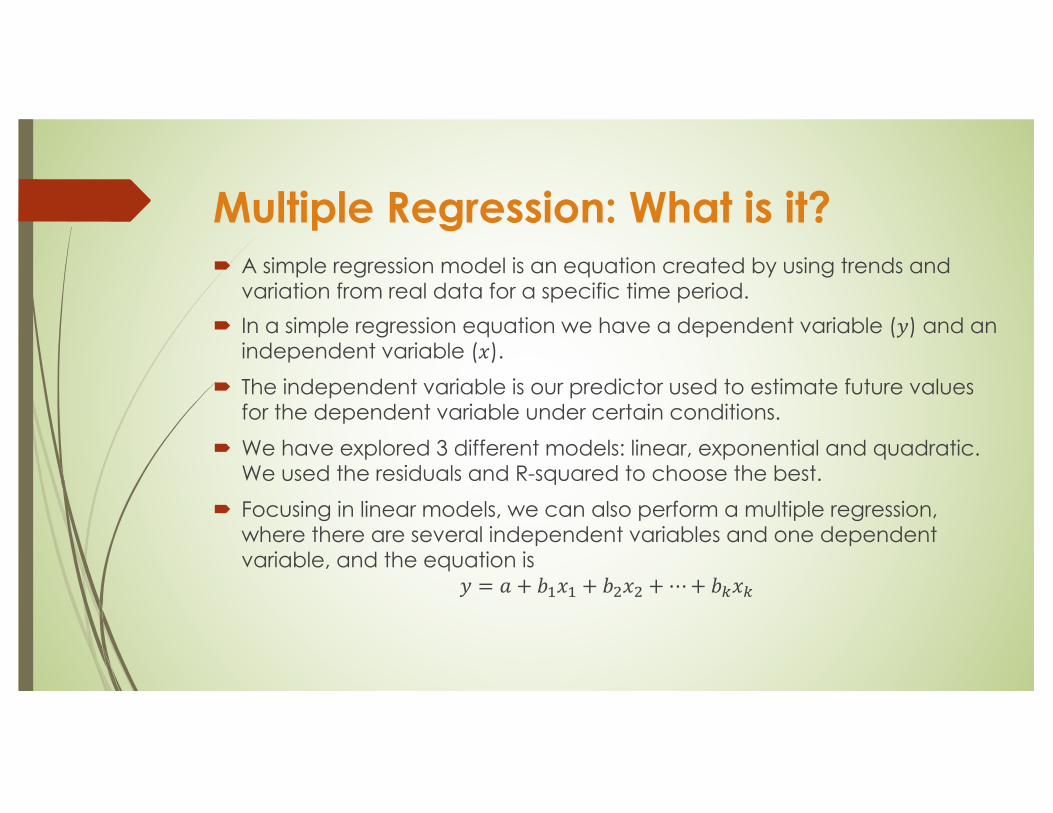
Multiple Regression: What is it?´ A simple regression model is an equation created by using trends and
variation from real data for a specific time period.´ In a simple regression equation we have a dependent variable (𝑦) and an
independent variable (𝑥). ´ The independent variable is our predictor used to estimate future values
for the dependent variable under certain conditions. ´ We have explored 3 different models: linear, exponential and quadratic.
We used the residuals and R-squared to choose the best. ´ Focusing in linear models, we can also perform a multiple regression,
where there are several independent variables and one dependent variable, and the equation is
𝑦 = 𝑎 + 𝑏'𝑥' + 𝑏(𝑥( +⋯+ 𝑏*𝑥*
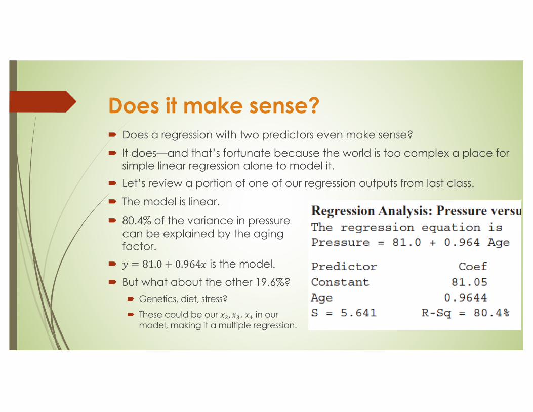
Does it make sense?´ Does a regression with two predictors even make sense? ´ It does—and that’s fortunate because the world is too complex a place for
simple linear regression alone to model it. ´ Let’s review a portion of one of our regression outputs from last class.´ The model is linear.
´ 80.4% of the variance in pressure can be explained by the aging factor.
´ 𝑦 = 81.0 + 0.964𝑥 is the model. ´ But what about the other 19.6%?
´ Genetics, diet, stress?
´ These could be our 𝑥(, 𝑥3, 𝑥4 in our model, making it a multiple regression.

For example… ´ If you know how to find the regression of %body fat on waist size, you can
usually just add height to the list of predictors without having to think hard about how to do it. ´ 𝑅( = 67.8%
´ For simple regression we found the Least Squares solution, the one whose coefficients made the sum of the squared residuals as small as possible.
´ For multiple regression, we’ll do the same thing but this time with more coefficients.

´ Remember:´ Equation
´ 𝑅(
´ P-values
´ 𝑦 = −3.10 + 1.77𝑥' − 0.60𝑥( or
´ 𝑅( gives the fraction of the variability of %body fat accounted for by the multiple regression model. ´ (With waist alone predicting %body fat, the was 67.8%.)
´ Waist size and height together account for about 71.3% of the variation in %body fat among men.
´ We shouldn’t be surprised that has gone up. It was the hope of accounting for some of that leftover variability that led us to try a second predictor.
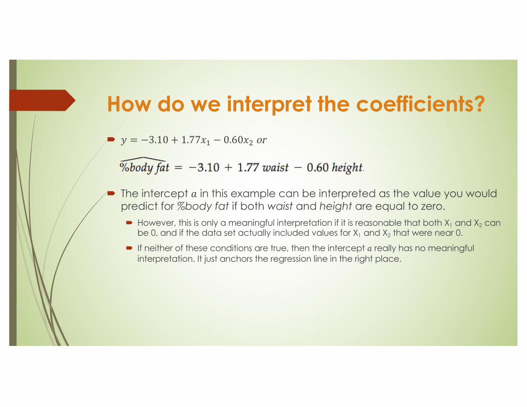
How do we interpret the coefficients?´ 𝑦 = −3.10 + 1.77𝑥' − 0.60𝑥( or
´ The intercept 𝑎 in this example can be interpreted as the value you would predict for %body fat if both waist and height are equal to zero. ´ However, this is only a meaningful interpretation if it is reasonable that both X1 and X2 can
be 0, and if the data set actually included values for X1 and X2 that were near 0.
´ If neither of these conditions are true, then the intercept 𝑎 really has no meaningful interpretation. It just anchors the regression line in the right place.

How do we interpret the coefficients?´ 𝑦 = −3.10 + 1.77𝑥' − 0.60𝑥( or
´ The first predictor 𝑏'𝑥'represents the difference in the predicted value of 𝑦for each one-unit difference in 𝑥', if 𝑥( remains constant.
´ The second predictor 𝑏(𝑥(represents the difference in the predicted value of 𝑦 for each one-unit difference in 𝑥(, if 𝑥' remains constant.
´ The regression equation indicates that each inch in waist size is associated with about a 1.77 increase in %body fat among men who are of a particular height.
´ Each inch of height is associated with a decrease in %body fat of about 0.60 among men with a particular waist size.
´ Both predictors are statistically significant!
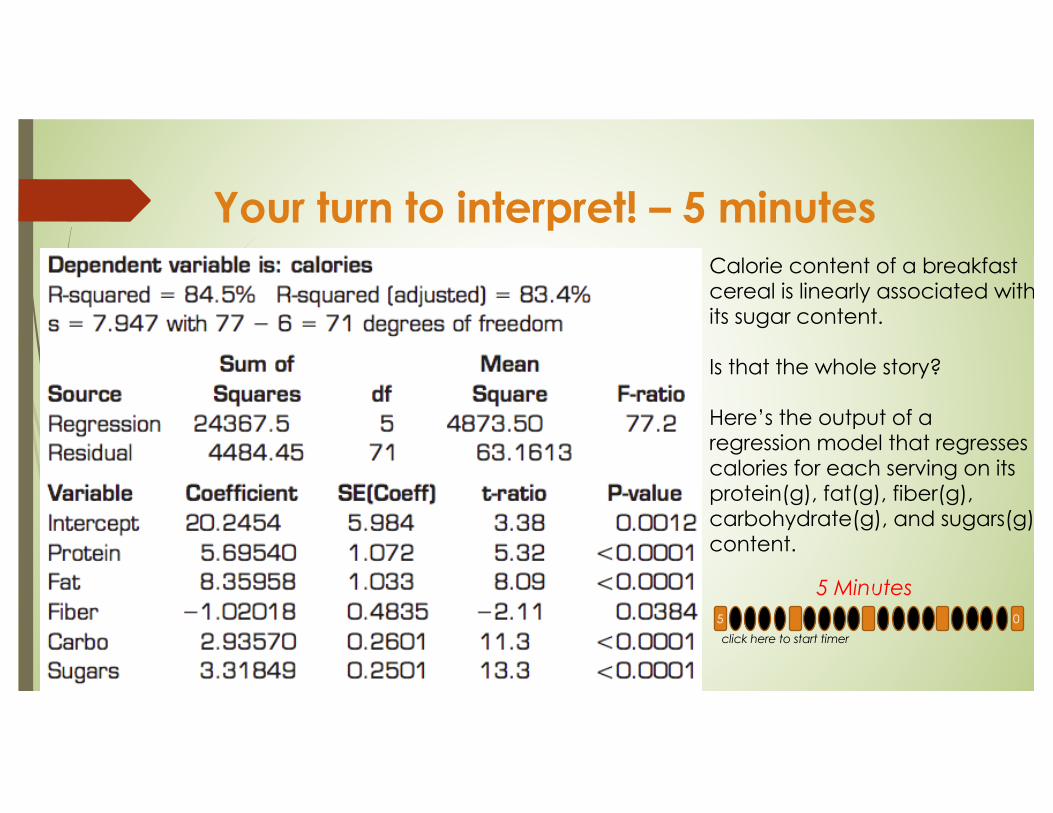
Your turn to interpret! – 5 minutesCalorie content of a breakfast cereal is linearly associated with its sugar content.
Is that the whole story?
Here’s the output of a regression model that regresses calories for each serving on its protein(g), fat(g), fiber(g), carbohydrate(g), and sugars(g) content.
5 Minutes5 0click here to start timer

Can we run it in desmos? ´ Sure we can, but we won’t have p-values.´ Follow the following steps:
´ Enter data in google spreadsheets or excel.
´ Name your variables.
´ Check for correlations between all possible pairs of variables.´ Ideally, your independent variables should have a low correlation between each other, but a
high correlation with the dependent.
´ Check for statistical significance.
´ If everything looks OK, copy the table in google and paste it in desmos.
´ Make sure your dependent in desmos is 𝑦' and your independent are 𝑥', 𝑥(, 𝑥3,etc.
´ In a new box type: 𝑦'~𝑎 + 𝑏'𝑥' + 𝑏(𝑥( (or keep adding if more variables, following the same format.
´ Interpret!

Try it!´ The nursing instructor wishes to see whether a student’s grade
point average and age are related to the student’s score on the state board nursing examination. She selects five students and obtains the following data.

Check your results!

Partner/Independent Work
´ Work on your worksheet. ´ If you do not finish today, please turn it in later.
´ Use your Chromebook or personal computer to complete all the calculation and graphing steps.
´ Open a google doc to add all your outputs and graphs.´ Save all your work in google and desmos.´ Make sure you keep everything in the same google doc.