Embed Size (px)
Citation preview

Statistics in astronomy and physics
Stephen Serjeant, Department of Physics and Astronomy These slides and some associated IDL code are available at http://physics.open.ac.uk/~sserjeant/statistics_lecture

Outline
The aim is to equip you with some handy statistical tools
that you may not have met in your undergraduate studies.
Some of this is stuff I wish I’d known as a PhD student.
• Introduction and some basic stuff • Kolmogorov-Smirnov tests• Matched filters - finding blobs in images • Multi-resolution techniques, e.g. wavelets • Sampling theory• Deconvolution techniques

Basic stuff• I’ll assume you’re already very familiar with
– what probability distributions are (or, more properly, probability density functions)
– cumulative distribution functions– the Gaussian, Poisson, and Binomial distributions 2 distribution, likelihood– expectation values, variances and covariances of independent
and dependent random variables – Monte Carlo simulations– the Central Limit Theorem – Fourier transforms and power spectra
• If not, go read an undergraduate statistics/maths book ASAP!

Basic stuff• What’s odd about these data streams?
• Moral: use (data-model)/noise or your signal-to-noise histogram to make sure your noise estimates are realistic!

Fourier Duck and Cat
• A duck and its Fourier transform (colours for phases, intensity for amplitudes)
Images taken from www.ysbl.york.ac.uk/~cowtan/fourier/fourier.html

Fourier Duck and Cat
• If we remove the high-frequency Fourier components and only keep the low resolution parts, we get a blurred duck. (Also note the ringing around the duck because we’ll come back to it in your homework.)
Images taken from www.ysbl.york.ac.uk/~cowtan/fourier/fourier.html

Fourier Duck and Cat
• If we only have the high resolution terms of the Fourier transform, we only see the edges of the duck.
Images taken from www.ysbl.york.ac.uk/~cowtan/fourier/fourier.html

Fourier Duck and Cat
• If some of the Fourier data is missing, then features perpendicular to the missing parts are blurred.
Images taken from www.ysbl.york.ac.uk/~cowtan/fourier/fourier.html

Fourier Duck and Cat
• A cat and its Fourier transform (colours for phases, intensity for amplitudes)
Images taken from www.ysbl.york.ac.uk/~cowtan/fourier/fourier.html

Fourier Duck and Cat
• Marrying cats and ducks! Magnitudes from duck, phases from cat.
Images taken from www.ysbl.york.ac.uk/~cowtan/fourier/fourier.html

Fourier Duck and Cat
• Marrying ducks and cats! Magnitudes from cat, phases from duck. This demonstrates the sorts of information in the Fourier amplitudes and phases. A Gaussian random field (e.g. primordial perturbations after Inflation) has random phases.
Images taken from www.ysbl.york.ac.uk/~cowtan/fourier/fourier.html

Fourier Duck and Cat
• Suppose we have a Fourier transform of a cat but only have the amplitudes, but don’t have the image to the left. How can we reconstruct the image to the left?
Images taken from www.ysbl.york.ac.uk/~cowtan/fourier/fourier.html
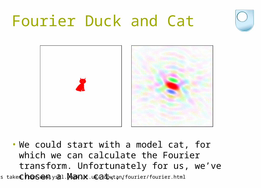
Fourier Duck and Cat
• We could start with a model cat, for which we can calculate the Fourier transform. Unfortunately for us, we’ve chosen a Manx cat...
Images taken from www.ysbl.york.ac.uk/~cowtan/fourier/fourier.html

Fourier Duck and Cat
• So, try the model phases plus the observed amplitudes to get a reconstructed image. Behold the tail! This is despite most structural information being in the phases, so the phases must be nearly right. But it’s at ~1/2 the correct weight. Also there is noise in the image.
Images taken from www.ysbl.york.ac.uk/~cowtan/fourier/fourier.html

Fourier Duck and Cat
• Next tweak the model. Factor of 1/2 occurs because we are making the right correction parallel to the estimated phase, but none perpendicular to the phase. So modify amplitudes (X-ray crystallography technique): |Fobs|2|Fobs|-|Fmodel|. Tail comes at full weight, but noise doubled.
Images taken from www.ysbl.york.ac.uk/~cowtan/fourier/fourier.html
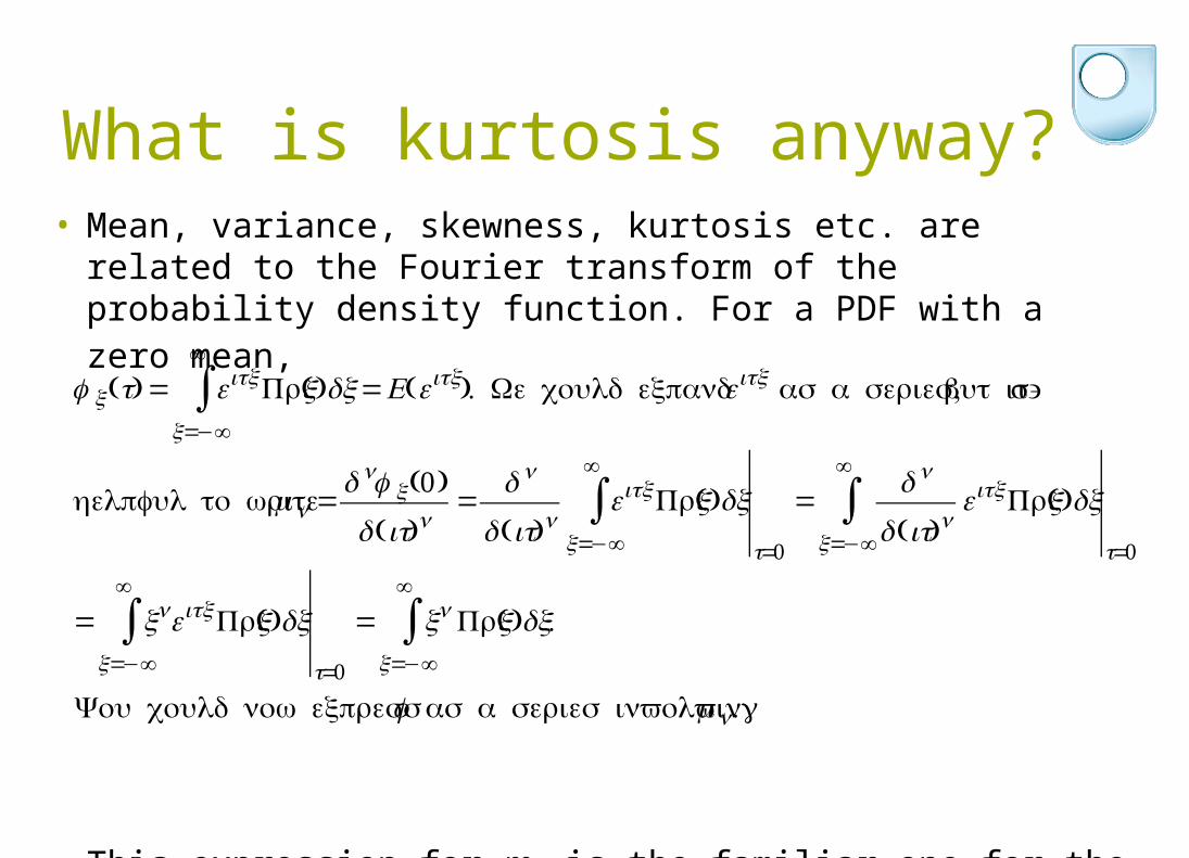
What is kurtosis anyway? • Mean, variance, skewness, kurtosis etc. are related to the Fourier
transform of the probability density function. For a PDF with a zero mean,
• This expression for mn is the familiar one for the nth moment. The first four moments are called mean, variance, skewness, kurtosis.
€
ϕ x(t) = eitx (Pr x)dxx=−∞
∞
∫ =E(eitx). We could expandeitx ,as a series but it' s
helpful to writemn=dnϕ x(0)
d(it)n= dn
d(it)neitx (Pr x)dx
x=−∞
∞
∫t=0
= dn
d(it)neitx (Pr x)dx
x=−∞
∞
∫t=0
= xneitx (Pr x)dxx=−∞
∞
∫t=0
= xn (Pr x)dxx=−∞
∞
∫ .
You could now expressϕ as a series involvingmn.

What is kurtosis anyway?
• This treatment can be generalised to the non-zero mean case. • Result: or for non-zero mean,
• Together, all the moments contain all the information on the PDF’s shape. (Why?)
x is known as the characteristic function. Some texts use the moment generating function, but I felt it makes the link to Fourier transform less obvious. It’s defined as:
(How are moments generated from
it?)
€
mn= xn
x=−∞
∞
∫ (Pr x)dx
€
mn= (x−μ)n
x=−∞
∞
∫ (Pr x)dx
€
M x(t) = etx (Pr x)dxx=−∞
∞
∫ =E(etx).

Kolmogorov-Smirnov Test• Is my data set consistent with my model? • Are my two data sets consistent?
fig. from arXiv:0712.3613
num
ber
(hat
ched
his
togr
am)
number (un-hatched histogram
)
Kolmogorov-Smirnov Test
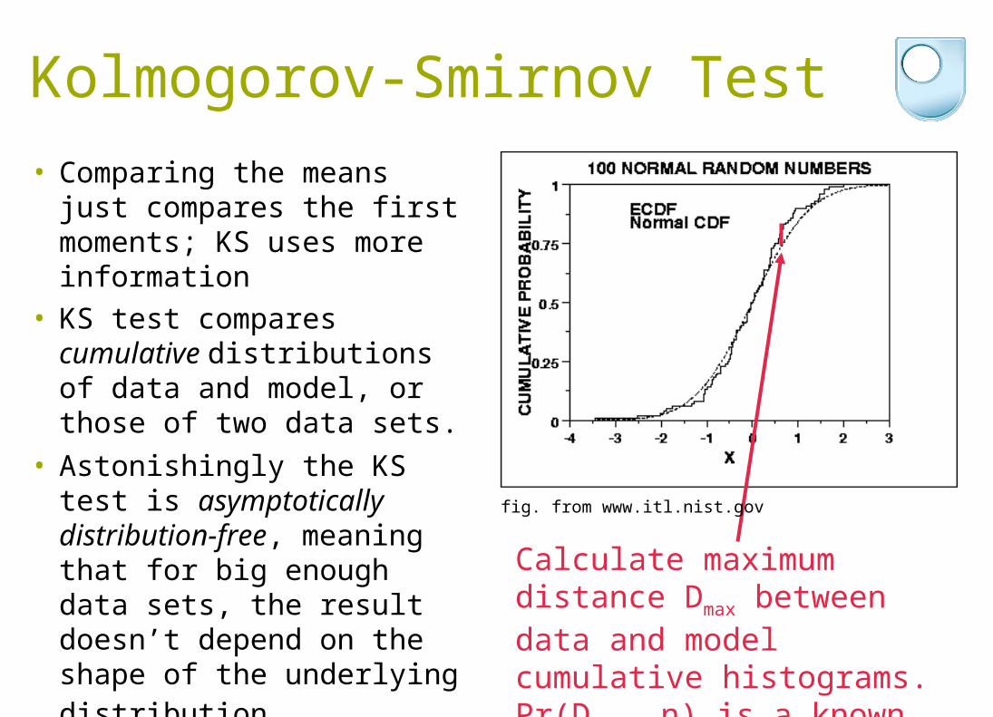
• Comparing the means just compares the first moments; KS uses more information
• KS test compares cumulative distributions of data and model, or those of two data sets.
• Astonishingly the KS test is asymptotically distribution-free, meaning that for big enough data sets, the result doesn’t depend on the shape of the underlying distribution.
• IDL: ksone.pro (data vs. model) & kstwo.pro (data1 vs. data2)
• Matlab: kstest & ranksum
Calculate maximum distance Dmax between data and model cumulative histograms. Pr(Dmax, n) is a known function.
fig. from www.itl.nist.gov

Kolmogorov-Smirnov Test• Example: stacking analysis.
Does my new deep image manage to detect some galaxies I’ve detected before?
• Can calculate mean flux at the galaxies’ positions (error from Central Limit Theorem):
• Also use KS test. Suppose galaxy positions are in IDL arrays x, y
IDL> data_on_my_galaxies = image[x,y]
IDL> kstwo, data_on_my_galaxies, image, dmax, prob
IDL> print, prob
fig. from arXiv:0712.3613
€
μ ±σ / n

2-D Kolmogorov-Smirnov Test• Four ways of making
cumulatives. Choose any one... • Significance levels have been
estimated using Monte Carlo simulations; unlike 1-D test, method is not based on analytic theory
• ‘Very nearly’ distribution-free: almost all the cases to the right give virtually identical results for sufficiently large samples
• See Peacock 1983 MNRAS 202, 615 for details
Fig. from Peacock 1983 MNRAS 202, 615

Matched filters
• Suppose we know there are features with Gaussian profiles in our data stream, with a known σ but unknown amplitude.
• What’s the best-fit profile for an object centred here? • Just minimise
€
2 = data-modelnoise
⎛
⎝ ⎜
⎞
⎠ ⎟2
x∑
= data-A×profilenoise
⎛
⎝ ⎜
⎞
⎠ ⎟2
x∑ = D(x)−Ap(x)
N(x)
⎛
⎝ ⎜
⎞
⎠ ⎟2
x∑
∂2
∂A=0, and solve forA

Matched filters
• What about the best-fit profile for an object centred here? • Same again - just minimise using a profile
centred somewhere else. We’ll call this profile p2.
€
2 = data-modelnoise
⎛
⎝ ⎜
⎞
⎠ ⎟2
x∑
= data-A×profilenoise
⎛
⎝ ⎜
⎞
⎠ ⎟2
x∑ = D(x)−Ap2(x)
N(x)
⎛
⎝ ⎜
⎞
⎠ ⎟2
x∑
∂2
∂A=0, and solve forA

Matched filters• What about having an array which gives you the best-fit
profile for an object centred anywhere? This time, use a new profile P which is N pixels wide:
• If N(x)=constant then A is just proportional to DP
• This is a minimum-variance (lowest noise) estimator for A
€
2(x) = data-modelnoise
⎛
⎝ ⎜
⎞
⎠ ⎟
i=−N /2
N /2
∑2
= D(x−i)−AP(i)N(x−i)
⎛
⎝ ⎜
⎞
⎠ ⎟2
i=−N /2
N /2
∑∂2
∂A=0, and solve forA, to find
A=
D(x−i)P(i)
N(x−i)2∑
P(i)2
N(x−i)2∑
=(D / N2 ) ⊗P
(1/ N2 ) ⊗P2 where⊗ denotes convolution
Note sum is now over i not x

Matched filters• So, ‘smoothing’ is related to
‘finding the best fit everywhere’
• Top image shows best-fits for two positions
• Bottom image shows best fit amplitude for all positions
• Why is the blue curve systematically higher in the middle than the data points?
• Generalised to 2-D and N(x)constant, e.g. Serjeant et al. 2003 MNRAS 344, 887
Min 2 does not necessarily mean the 2 is any good!

Matched filters
• 2-D example: SHADES 850μm image of the Subaru-XMM Deep Field
• Image greyscales from -2σ to 6.6σ
• Signal-to-noise histogram shows– the noise is realistic (histogram
is roughly a Gaussian with zero mean and unit variance)
– an excess at positive fluxes, due to the objects in the field
Images from data analysed in Mortier et al. 2005 MNRAS 363, 563; combines images with several PSFs
Before matched filter

Matched filters
• 2-D example: SHADES 850μm image of the Subaru-XMM Deep Field
• Image greyscales from -2σ to 6.6σ
• Signal-to-noise histogram shows– the noise is realistic (histogram
is roughly a Gaussian with zero mean and unit variance)
– an excess at positive fluxes, due to the objects in the field
After matched filtering by point spread functions*
* PSF = instrumental resolution = response of detector to an unresolved (delta-function) object
6.66.6σσ source (honest!) source (honest!)
Images from data analysed in Mortier et al. 2005 MNRAS 363, 563; combines images with several PSFs

Matched filters
• 2-D example: SHADES 850μm image of the Subaru-XMM Deep Field
• Image greyscales from -2σ to 6.6σ
• Signal-to-noise histogram shows– the noise is realistic (histogram
is roughly a Gaussian with zero mean and unit variance)
– an excess at positive fluxes, due to the objects in the field
Signal-to-noise of matched filtered image*
* Noise on filtered image can be calculated by propagating errors on DP, e.g. Serjeant et al. 2004 MNRAS 344, 887; Mortier et al. 2005 MNRAS 363, 563Images from data analysed in Mortier et al. 2005
MNRAS 363, 563; combines images with several PSFs

Matched filters on clumpy backgrounds
• See e.g. Vio et al. 2002 A&A 391, 789• NB minimum-variance does not necessarily mean
highest-reliability or highest-completeness
€
Fourier transform of minimum- variance filter is
(k)∝ τ(k)P(k) whereτ(k) is FT of PSF andP(k)
is background power spectrum
Note negative side-lobes give a local sky subtraction; similar to (or in some cases identical to) Mexican Hat Wavelet - see later.
Real space Fourier space

Matched filters on clumpy backgrounds
Figs. by Ho Seong Hwang
IRAS 60μm sample data

Multi-resolution techniques• Convolve time stream with
progressively bigger kernel
• Stack these 1-D convolved signals to make a 2-D image
• Look for features in this 2-D plane
• Advantage over Fourier analysis: sharp changes are localised in position as well as frequency
• www.amara.com/current/wavelet.html Figures from P. Addison, Physics World, March 2004

Multi-resolution techniques
Figures from P. Addison, Physics World, March 2004

• Starck et al. 1999 A&AS 138, 365 used a boxcar median filter rather than a convolution kernel
• They also use differences from scale to scale, rather than the measurements themselves at each scale (a very effective touch)
• Multi-resolution decomposition of images 3-D data cube in which features are identified Fig. from Starck et al. 1999 A&AS 138, 365
Multi-resolution techniques

Multi-resolution techniquesThis data stream from one pixel...
...is decomposed into its components...
...unwanted signals are removed (detector glitches) leaving this cleaned signal:
Figs. from Starck et al. 1999 A&AS 138, 365

Multi-resolution techniques• Amara Graps has an excellent wavelet page
www.amara.com/current/wavelet.html with links to:– Mathcad wavelet extension pack– Mathematica wavelet programs – IDL wavelet utilities in IDL Wavelet Toolkit (add-on to
IDL)

Sampling theory• Nyquist-Shannon sampling theory:
– Suppose a function f(x) has a Fourier transform F(k) that is zero above some scale k>k0
– Then f can be completely specified if it is sampled at regular intervals no wider than (2k0)-1 (Nyquist sampling)
Astronomers’ pixels are usually ~half the FWHM or smaller
• Sampling more coarsely than this (“undersampling”) loses information & can create artefacts
• Undersampled detectors (e.g. HST WFC, SCUBA) need dithering
• Finer sampling than Nyquist referred to as “oversampling” Images from wikipedia.org/wiki/Moire

Confusion limit • Sufficiently deep astronomical
images are a crowded field of blended sources
• RMS from this ‘background’ dominated by objects with number density of about 1 per point spread function
• Effective limit for source extraction is determined by the desired significance (e.g. 3σ, 5σ) and number counts dN/dS
• In astronomy, usually 1 source per 20-40 beams is reasonable for a 5σ confusion-limited catalogue
Fig. shows NICMOS image of the Galactic Centre, from ssc.spitzer.caltech.edu. See e.g. Condon 1974 ApJ 188, 279; Väisänen et al. 2001 MNRAS 325, 1241 & refs. therein
Deconvolution
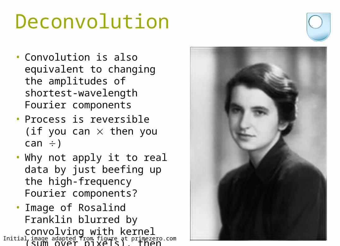
• Convolution is also equivalent to changing the amplitudes of shortest-wavelength Fourier components
• Process is reversible (if you can then you can )
• Why not apply it to real data by just beefing up the high-frequency Fourier components?
• Image of Rosalind Franklin blurred by convolving with kernel (sum over pixels), then restored by amplifying some high-frequency Fourier components
Initial image adapted from figure at primezero.com
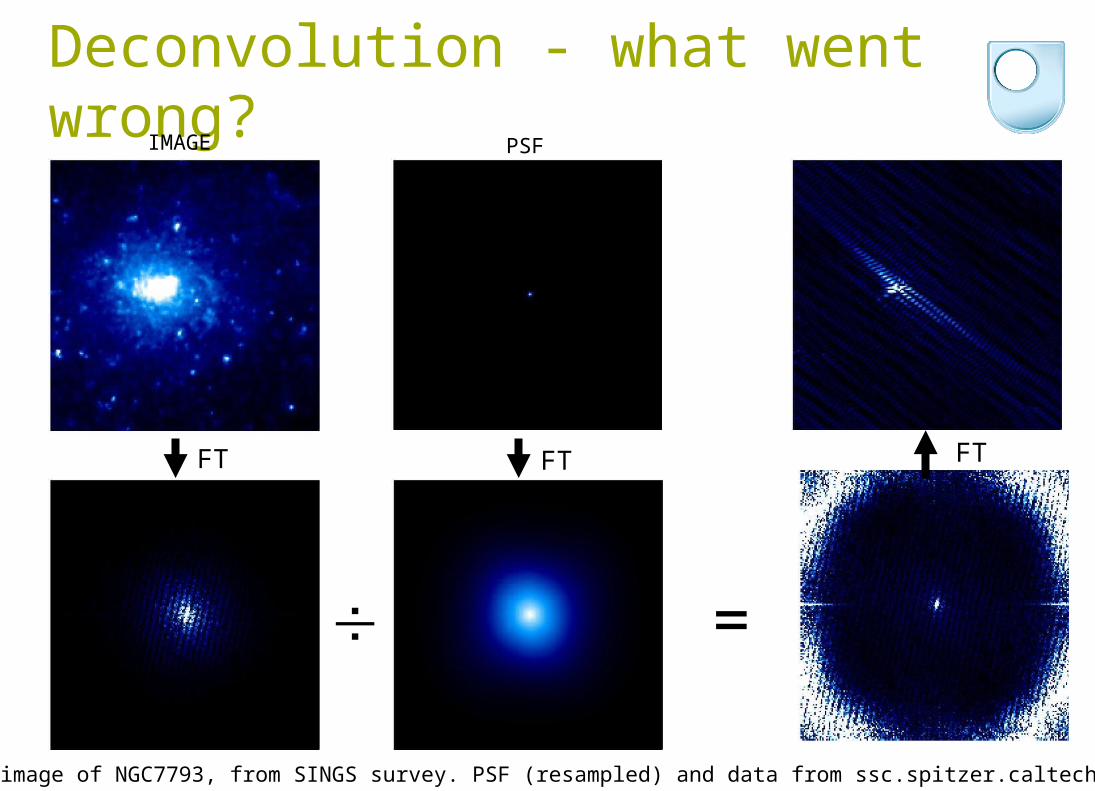
Deconvolution - what went wrong?
FT FT
=
FT
3.6μm image of NGC7793, from SINGS survey. PSF (resampled) and data from ssc.spitzer.caltech.edu
IMAGE PSF

Deconvolution - what went wrong?• Moral: need sufficient signal-to-noise in Fourier
components • A Gaussian PSF is also a Gaussian in Fourier space so
high-frequency components are suppressed by a factor ~exp(-0.5(k/k0)2)
• Even in my Rosalind Franklin deconvolution earlier, digitisation error crept in on the smallest scales so not all Fourier modes could be boosted
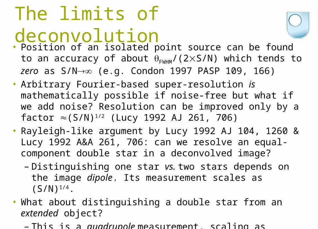
The limits of deconvolution• Position of an isolated point source can be found to an accuracy of
about FWHM/(2S/N) which tends to zero as S/N (e.g. Condon 1997 PASP 109, 166)
• Arbitrary Fourier-based super-resolution is mathematically possible if noise-free but what if we add noise? Resolution can be improved only by a factor (S/N)1/2 (Lucy 1992 AJ 261, 706)
• Rayleigh-like argument by Lucy 1992 AJ 104, 1260 & Lucy 1992 A&A 261, 706: can we resolve an equal-component double star in a deconvolved image? – Distinguishing one star vs. two stars depends on the image
dipole. Its measurement scales as (S/N)1/4. • What about distinguishing a double star from an extended object?
– This is a quadrupole measurement, scaling as (S/N)1/8.
• These are formidable barriers! But gains appear better if assuming a model (e.g. quasar host galaxies, gravitational lenses).

The limits of deconvolution
Cloverleaf quasar observed with ESO 2.2m telescope (figure from Magain et al. 1998 ApJ 494, 472). Left: observed image with FWHM 1.3’’. Right: deconvolved image with 0.5’’ resolution, made assuming the image is made of a number of point sources. But note that we don’t necessarily have information at 0.5’’ resolution everywhere in the image.

CLEAN deconvolution• Interferometry only samples a small part of the Fourier plane (known
as u-v plane in astronomy). This means the point spread function has lots of features (“dirty beam”) unlike desired Gaussian or Airy function (“clean beam”)
• Radio telescopes collect both amplitudes and phases (unlike e.g. X-ray crystallography which is just amplitudes)
• CLEAN uses iterative model to predict amplitudes and (for interferometry) phases:
1. find peak in dirty image
2. subtract dirty beam scaled by peak strength and (user-selected) loop gain
3. add corresponding source to model (initially empty)
4. go to 1 unless any remaining peak is below user-selected threshold
5. convolve model with desired clean beam, and add to residual map

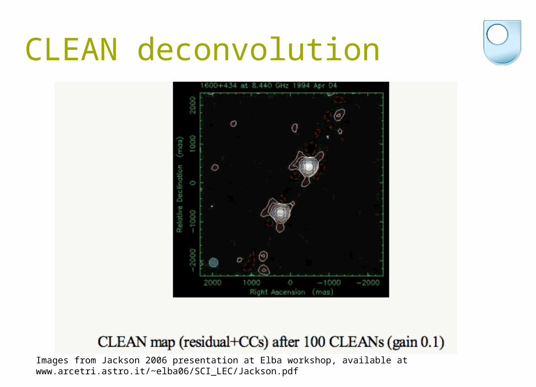
CLEAN deconvolution
Images from Jackson 2006 presentation at Elba workshop, available at www.arcetri.astro.it/~elba06/SCI_LEC/Jackson.pdf Description of CLEAN (previous slide) from Saunders 2002 presentation at 2nd APC workshop, available at www.apc.univ-paris7.fr/APCP7_new/aapc/atelier2002.html
Recall stripy blurring in Fourier Duck when Fourier coverage incomplete

CLEAN deconvolution
Images from Jackson 2006 presentation at Elba workshop, available at www.arcetri.astro.it/~elba06/SCI_LEC/Jackson.pdf

CLEAN deconvolution
Images from Jackson 2006 presentation at Elba workshop, available at www.arcetri.astro.it/~elba06/SCI_LEC/Jackson.pdf
CLEAN deconvolution
Images from Jackson 2006 presentation at Elba workshop, available at www.arcetri.astro.it/~elba06/SCI_LEC/Jackson.pdf

Richardson-Lucy deconvolution
• Assume the data di and the true sky sj are related by the point spread function pij:
• Using Bayes’ Theorem, can derive an iterative scheme for finding the most probable model for the sky uj:
• The result of each iteration is used to make a prior for the next one
• No general convergence proof but works well in simulations. See e.g. Lucy 1974 AJ 79, 745; Richardson 1972 JOSA 62, 55
€
di = pijj∑ sj
€
ui(t+1) =ui
(t) d j
D jj∑ pij whereD j = uk
(t)
k∑ pjk

Richardson-Lucy deconvolution• Implemented in IRAF: stsdas.contrib.plucy• IDL implementation part of NICMOS library • Matlab: deconvlucy.m in image toolbox • Starlink: LUCY
Fig. from White 1994 SPIE 2198, 1342 of RL deconvolution of HST image of Saturn. White also discusses noise reduction in RL deconvolution.

Maximum Entropy deconvolution• Another Bayesian technique• Aim is to minimise a “smoothness” function proportional
to the Shannon entropy, i.e. to find the minimum information content (defined in the Shannon sense) that is consistent with the data
• This method finds an image b which is as close as is allowed by the data to a prior estimate m (subject to the constraint that 2 equals its expected value):
• See e.g. Cornwell & Evans 1985 A&A 143, 77 • Noise analysis possible (unlike CLEAN)Shannon’s original 1948 paper on entropy and information is accessibly written and is available at http://www-db-out.research.bell-labs.com/cm/ms/what/shannonday/shannon1948.pdf
€
Entropy=H =− bi (ln bi /mi )i pixels
∑
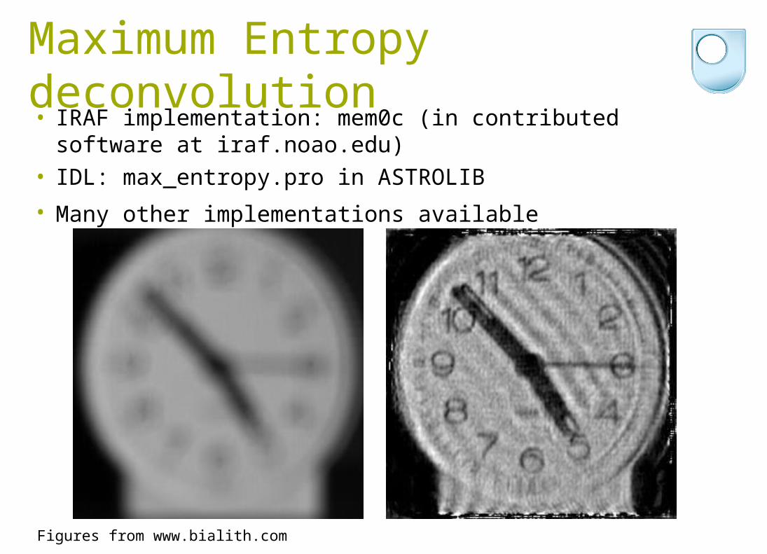
Maximum Entropy deconvolution
Figures from www.bialith.com
• IRAF implementation: mem0c (in contributed software at iraf.noao.edu)
• IDL: max_entropy.pro in ASTROLIB
• Many other implementations available

Emerson-II deconvolution
• Submm astronomical observations often “chopped” to help sky subtraction (sky is often ~105-106 times brighter than targets of interest)
• Fourier modes on chop scale therefore lost
Figs. from Jenness et al. 2000 ASP 216, 559, available at www.adass.org/adass/proceedings/adass99/P2-56/ and from SUN216 available at starlink.rl.ac.uk
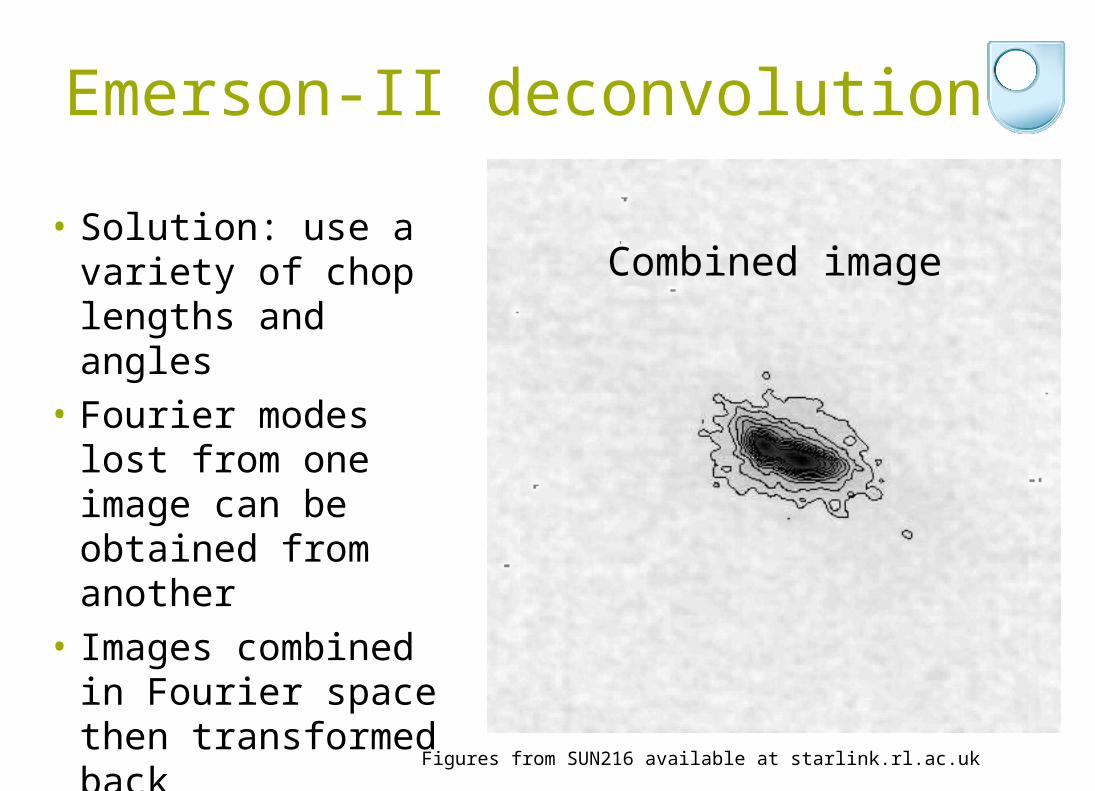
Emerson-II deconvolution
• Solution: use a variety of chop lengths and angles
• Fourier modes lost from one image can be obtained from another
• Images combined in Fourier space then transformed back
• See e.g. Jenness et al. 2000 ASP 216, 559
Figures from SUN216 available at starlink.rl.ac.uk
Combined image

MADMAP
• Assume detector is scanning across the sky, with nt time samples at ns spatial positions
• Assume data time stream d has fluctuations n from piecewise stationary Gaussian noise (which can include 1/f noise)
• Define matrix A of size ntns to map positions as a function of time onto the sky positions.
• Define time-time noise covariance matrix of data to be matrix N (dimensions ntnt)
• Then: d = n + As• This has maximum-likelihood solution for the sky image:
m = (ATN -1A)-1ATN -1d• MADMAP solves this equation. It was developed for CMB map
reconstruction - see http://crd.lbl.gov/~cmc/MADmap/doc/

MADMAP• Image shows simulated data from
Herschel Space Observatory (Waskett et al. 2007 MNRAS 381, 1583)
• Two scan directions used • Detector has long timescale drifts
that can be seen in the scan directions
• MADMAP isolates the true sky signal (invariant with position) from the artefacts (which depend on scan time and not sky position)
• NB enough multiple observations (“redundancy”) and all noise is gaussian-ized by Central Limit Theorem (essential for SCUBA)

Astro background for your homework
• Ground-based optical telescopes’ resolution limited by seeing (the blurring due to atmospheric turbulence)
• In space, no atmosphere diffraction limit obtainable
• Point spread function is closely related to the Fourier transform of the telescope aperture (from your undergraduate optics)
• PSF is Airy function (e.g. recall Fourier Duck’s truncated FT)
F.T.
Figs from www.cs.cf.ac.uk/Dave/Vision_lecture/Vision_lecture_caller.html and Krist et al. 2005 AJ 130, 2778
HST image of star GGTau and its companion (logarithmic greyscale). Diffraction spikes etc. caused by e.g. struts in HST’s optics
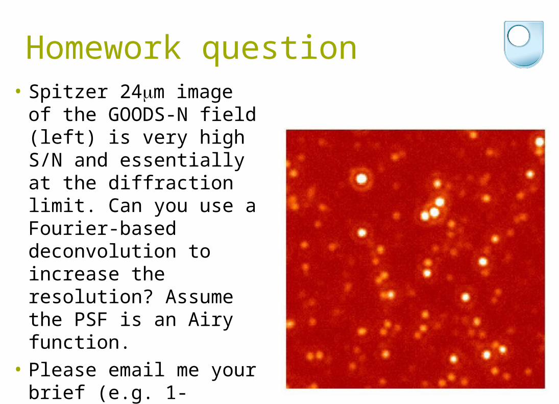
Homework question• Spitzer 24μm image of the
GOODS-N field (left) is very high S/N and essentially at the diffraction limit. Can you use a Fourier-based deconvolution to increase the resolution? Assume the PSF is an Airy function.
• Please email me your brief (e.g. 1-sentence, but not 1-word) answers by this time next week!

Summary• Moments of a PDF contain all the information on the
PDF’s shape• Try statistics that use more than just the first moment,
e.g. Kolmogorov-Smirnov• “Finding the min-2 model everywhere” is equivalent to
convolution • Convolution itself equivalent to a multiplication in Fourier
space • Many useful techniques are available for restoring the
information suppressed in convolution• Impressive results can be had from model-dependent
deconvolution but don’t forget the model dependence

Last thoughts
• 60% of people believe in God (UK MORI poll 2003, www.ipsos-mori.com/polls/2003/bbc-heavenandearth.shtml)
• 64% of people don’t trust statistics (UK ONS poll 2008, www.statistics.gov.uk/pdfdir/pco0308.pdf)
• 88.2% of statistics are made up on the spot (Vic Reeves, news.bbc.co.uk/1/hi/uk/859476.stm)