Statistics IIComputer Lab 2: Simple and multiple linear

regression analysis

Objectives

During this computer lab we will analyze the Spanish employment dataas a function of the GDP (and education), grouped by ’ComunidadesAutonomas’. In particular we will:

I Fit a linear regression model for employment on GDP and educationand assess the significance of the model parameters

I Make predictions based on the fitted model

I Perform diagnostic checks

Data

Our data set, which can be downloaded from INE (Instituto Nacional deEstadıstica) website http://www.ine.es, corresponds to the years 2008and 2009 and contains the following indicators/variables (grouped by’Comunidades’):

I Employment rate (column ’Employment’)

I GDP per capita (column ’GDP’)

I Percentage/proportion of the population with a university diploma(column ’HigherEdu’)

I Percentage/proportion of the population with a PhD title (column’PhD’)

This data set is also available on the course website:’DataRegAcc12.xlsx’. Choose the 2nd spreadsheet.

Downloading the data

• To download the datafrom the Internet:

I Go to:http://www.ine.es

I At the top of thepage, click on tabnumber 2:’INEbase’

Scatterplot in Excel• To plot y versus x.

I Highlight bothboth datacolumns.

I Go to ’Insert’ andthen choose’Scatter’ and hitOK

By default, the firstcolumn will be set to x.To swap the variablesaround:

I Left-click on theplot, thenright-click.

I From the dialogwindow, choose’Select data’ andthen ’Edit’.

Data Analysis

• To analyze the data,we will use Excel’sadd-in called ’DataAnalysis’.Make sure it is loaded:

I In the menu ’Data’

I It should appearon the right as’Data Analysis’

If it is not loaded,check Comp Lab 1notes.

Simple Linear Regression Analysis• To fit a simple linear regression model in Excel go to:

I Menu ’Data’ and submenu ’Data Analysis’

I From the dialog window, choose ’Regression’

I Choose data ranges for the dependent (y = employment) andindependent (x = GDP) variables

I Output for the results

I Confidence level, etc

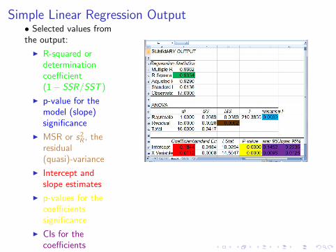
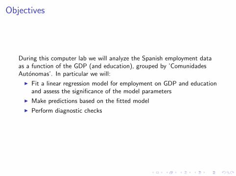
Simple Linear Regression Output• Selected values fromthe output:

I R-squared ordeterminationcoefficient(1− SSR/SST )

I p-value for themodel (slope)significance

I MSR or s2R , the

residual(quasi)-variance

I Intercept andslope estimates

I p-values for thecoefficientssignificance

I CIs for thecoefficients

Interpretation of the regression results

I What is the equation of the fitted model?

y = 0.184 + 0.0112x

I What is the value of the determination coefficient?

R2 = 0.9334 = 93.34%

Note that this coefficient is close to 100%.

I Is the model significant? ⇔ Is the linear dependence of y on xstatistically significant? ⇔ In a two-sided test, is H0 : β1 = 0rejected?

p-value = 0.0000

Note that the p-value is extremely small.

I 95% confidence interval for the population slope:

CI0.95(β1) = (0.0095, 0.0128)

Note that 0 is outside this interval.

Prediction interval

• We want topredict/estimate (withconfidence) the value of yfor x0 = 22.32.

I Estimated value of yis y0 = 0.184 +0.0112(22.32) =0.434

I Standard error is SE =√s2R

(1 + 1

n + (x0−x)2

(n−1)s2X

)I 95% prediction

interval isy0 ∓ t15;0.025 · SE

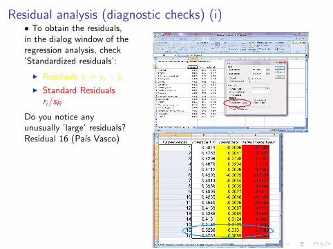
Residual analysis (diagnostic checks) (i)• To obtain the residuals,in the dialog window of theregression analysis, check’Standardized residuals’:

I Residuals ri = yi − yi

I Standard Residualsri/sR

Do you notice anyunusually ’large’ residuals?Residual 16 (Paıs Vasco)

Residual analysis (diagnostic checks) (ii)• To obtain the residualplot, in the dialog windowof the regression analysis,check ’Residual Plots’.Look for any suspiciouspatterns in the plot:

I Nonlinearity

I Heteroscedasticity

Residual analysis (diagnostic checks) (iii)• To obtain the normalprobability plot of theresiduals, in the dialogwindow of the regressionanalysis, check ’NormalProbability Plots’:

I It shows normalpercentiles versussample percentiles(very similar toQQ-plot fromStatistics I)

I Should follow astraight line if theresiduals follow anormal distribution

I Look for anysuspicious deviationsof the points from thestraight line

Multiple Linear Regression Analysis• To fit a multiple linear regression model in Excel go to:

I Menu ’Data’ and submenu ’Data Analysis’I From the dialog window, choose ’Regression’I Choose data ranges for the dependent (y = employment) and

independent (x1 = GDP and x2 = HigherEdu) variables. Note: theindependent data range covers two columns.

I Output for the resultsI Confidence level, etc

Regression Output• Selected values fromthe output:

I AdjustedR-squared ordeterminationcoefficient(1−MSR/MST )

I p-value for theglobal modelsignificance

I MSR or s2R , the

residual(quasi)-variance

I (Individual)coefficientsestimates

I p-values for the(individual)coefficientssignificance

I CIs for the(individual)coefficients

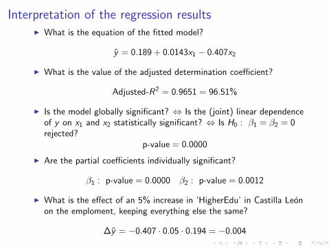
Interpretation of the regression resultsI What is the equation of the fitted model?

y = 0.189 + 0.0143x1 − 0.407x2

I What is the value of the adjusted determination coefficient?

Adjusted-R2 = 0.9651 = 96.51%

I Is the model globally significant? ⇔ Is the (joint) linear dependenceof y on x1 and x2 statistically significant? ⇔ Is H0 : β1 = β2 = 0rejected?

p-value = 0.0000

I Are the partial coefficients individually significant?

β1 : p-value = 0.0000 β2 : p-value = 0.0012

I What is the effect of an 5% increase in ’HigherEdu’ in Castilla Leonon the emploment, keeping everything else the same?

∆y = −0.407 · 0.05 · 0.194 = −0.004

Additional exercises (i)

Once you completed the above exercises for 2008, focus on year 2009and:

I Fit a simple linear regression model for y on x

I How do the parameter estimates for 2009 compare to those for2008, i.e., is there a big change?

I Fit a multiple linear regression model for y on x1 and x2

I Was there a big change in the coefficient of x2 between 2009 and2008?

Additional exercises (ii)

I For 2008, fit a multiple linear regression model for employment onGDP (x1) and the percentage of population with a PhD title (x2)

I Is the model globally significant?

I Is the coefficient of x2 significant?