Statistics 67 Introduction to Probability and Statistics ...sternh/courses/67/stat67slides.pdf · Introduction to Probability and Statistics for Computer Science Lecture notes for

Statistics 67Introduction to Probability and Statistics

for Computer Science

Lecture notes for Statistics

Hal SternUniversity of California, Irvine

[email protected]

1

From Probability ....

• To this point

– probability as a measure of uncertainty

– probabilities for events∗ axioms, probability rules,

conditional probability, Bayes’ rule

– random variables as quantities of interest in anuncertain environment

– probability distributions as descriptions of possiblevalues for a random variable along with anassessment of how likely each value is to occur

∗ discrete/continuous distributions∗ univariate/multivariate distributions∗ joint, marginal, conditional distributions∗ expected values (mean, variance, covariance)

– sampling/simulation as ways of studying apopulation or distribution

2

.... to Statistical Inference

• Goal for remainder of quarter is to use what we knowabout probability to help us analyze data in scientificstudies

– use a sample from the population to learn aboutcharacteristics of the population

– a common approach is to assume that observedsample are independent observations from apopulation model (e.g., Poisson or normal)

– estimate the parameter(s) of the assumed model(e.g., normal mean or binomial proportion)

– check fit of the assumed probability model

– draw conclusions based on the estimated parameters(if appropriate)

3

Point Estimation

• Importance of how data are obtained

– we don’t discuss in detail here how our data arecollected

– for statistical methods to be valid we need thesample to be representative of the population we arestudying

– typically this involves the use of randomness orchance in selecting the sample to avoid biasedselections

– a simple random sample is the most basic approachand that is what we assume

– more sophisticated methods (multistage sampling,cluster sampling) can be accommodated

4

Point Estimation

• Estimand – the quantity being estimated

• We can think of two types of estimands

– Finite population summaries∗ mean of a finite population∗ variance of a finite population

– Parameters in a mathematical model of a population(can think of as an infinite population)∗ µ or σ2 in a Normal distribution∗ λ (mean = variance) of Poisson distribution∗ p in a binomial distribution

• For the most part we focus on parameters in amathematical model of a population

5

Point Estimation

• Basic Approach

– suppose θ is a parameter that we are interested inlearning about from a random sampleX1, X2, . . . , Xn

– e.g., θ might be the mean of the population that weare interested in (µX)

– θ, a point estimator, is some function of the datathat we expect will approximate the true value of θ

– e.g., we might use µ = X to estimate the mean of apopulation (µX)

– once we collect data and plug in we have a pointestimate x

– point estimator is the random variable (or function)and point estimate is the specific instance

• Two key questions are

1. How do we find point estimators?

2. What makes a good estimator?

6

Point Estimation - basics

• Assume we have a sample of independent randomvariables X1, X2, ..., Xn, each assumed to have densityf(x)

• We call this a random sample (or iid sample) from f(x)

• Assume the density is one of the families we haveconsidered which depends on one or more parameters θ;we usually write the density as f(x|θ)

• Goal is to estimate θ. Why?

– f(x|θ) is a description of the population

– θ is often an important scientific quantity (e.g., themean or variance of the population)

7

Point EstimationMethod of moments

• Recall E(Xj) is the jth moment of the population (orof the distribution); it is a function of θ

• The jth moment of the sample is 1n

∑i Xj

i

• We can equate the sample moment and the populationmoment to identify an estimator

• Suppose that there are k parameters of interest (usuallyk is just one or two)

• Set first k sample moments equal to first k populationmoments to identify estimators

• This is known as the method of moments approach

8

Point EstimationMethod of moments

• Example: Poisson case

– suppose X1, X2, . . . , Xn are a random sample fromthe Poisson distribution with parameter λ

– recall that E(Xi) = λ

– the method of moments estimator is obtained bytaking the first sample moment (X = 1

n

∑i Xi) equal

to the first population moment λ to yield λ = X

– V ar(Xi) is also equal to λ so it would also bepossible to take the sample variance as an estimateof λ (thus method of moments estimates are notunique)

9

Point estimationMethod of moments

• Example: Normal case

– suppose X1, X2, . . . , Xn are a random sample fromthe normal distribution with parameters µ and σ2

– recall that E(Xi) = µ and E(X2i ) = σ2 + µ2

– to find method of moments estimators we need tosolve

1n

n∑

i=1

Xi = µ

1n

n∑

i=1

X2i = σ2 + µ2

– results:

µmom =1n

n∑

i=1

Xi = X

σ2mom =

1n

n∑

i=1

(Xi − X)2

• Method of moments summary

– easy to use

– generally not the best estimators

– some ambiguity about which moments to use

10

Point EstimationMaximum likelihood estimation

• The density of a single observation is f(x|θ)• The joint density of our random sample is

f(X1, X2, . . . , Xn|θ) =∏n

i=1 f(Xi|θ)(recall the Xi’s are independent)

• This joint density measures how likely a particularsample is (assuming we know θ)

• Idea: look at the joint distribution as a function of θ

and choose the value of θ that makes the observedsample as likely as possible

• Likelihood function = L(θ|x1, . . . , xn) = f(x1, . . . , xn|θ)• Maximum likelihood estimator θmle is the value of θ

that maximizes the likelihood function

11


• To find the MLE:

– solve dL/dθ = 0 to identify stationary point

– check that we have a maximum(can use the 2nd derivative)

– it is often easier to maximize the logarithm of thelikelihood(which is equivalent to maximizing the likelihood)

– in complex models it can be hard to find themaximum

12


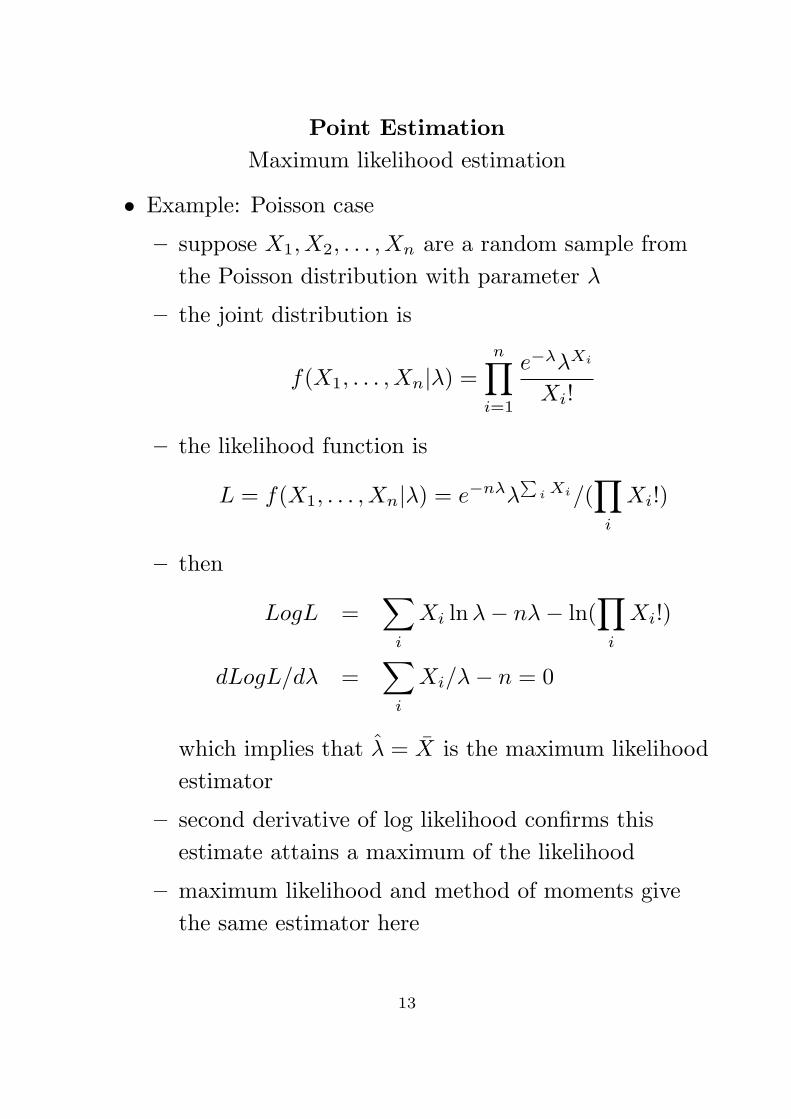
• Example: Poisson case

– suppose X1, X2, . . . , Xn are a random sample fromthe Poisson distribution with parameter λ

– the joint distribution is

f(X1, . . . , Xn|λ) =n∏

i=1

e−λλXi

Xi!

– the likelihood function is

L = f(X1, . . . , Xn|λ) = e−nλλ∑

i Xi/(∏

i

Xi!)

– then

LogL =∑

i

Xi ln λ− nλ− ln(∏

i

Xi!)

dLogL/dλ =∑

i

Xi/λ− n = 0

which implies that λ = X is the maximum likelihoodestimator

– second derivative of log likelihood confirms thisestimate attains a maximum of the likelihood

– maximum likelihood and method of moments givethe same estimator here

13


• Example: normal case

– suppose X1, X2, . . . , Xn are a random sample fromthe Normal distribution with mean µ, variance σ2

– LogL = constant− n2 log σ2 − 1

2σ2

∑ni=1(Xi − µ)2

– need to solve

∂LogL/∂µ =1σ2

n∑

i=1

(Xi − µ) = 0

∂LogL/∂σ2 = − n

2σ2+

12σ4

n∑

i=1

(Xi − µ)2 = 0

– results (same estimators as method of moments)

µmle =1n

∑

i

Xi = X

σ2mle =

1n

∑

i

(Xi − X)2

• Maximum likelihood summary

– more complex than method of moments

– statistical theory (not covered) suggests thatmaximum likelihood estimates do well (especiallywith lots of data)

14

Point EstimationProperties of point estimators

• Now have two methods for finding point estimators

• What makes for a good estimator?

– suppose T (X1, . . . , Xn) is an estimator of θ

– traditional approach to statistics asks how well T

would do in repeated samples

– key to studying estimators is to note that T is itselfa random variable and we can study properties of itsdistribution

– examples of good properties include

∗ lack of bias∗ low variance

15


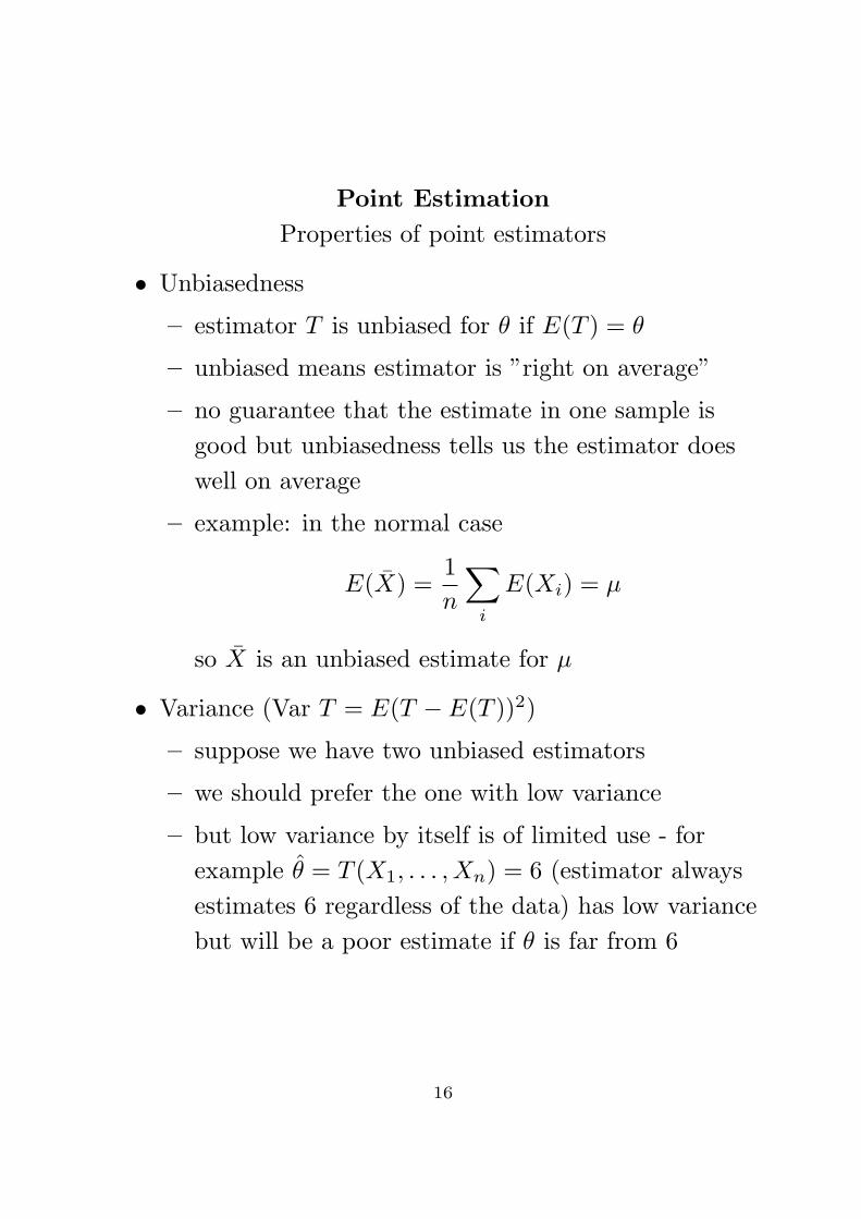
• Unbiasedness

– estimator T is unbiased for θ if E(T ) = θ

– unbiased means estimator is ”right on average”

– no guarantee that the estimate in one sample isgood but unbiasedness tells us the estimator doeswell on average

– example: in the normal case

E(X) =1n

∑

i

E(Xi) = µ

so X is an unbiased estimate for µ

• Variance (Var T = E(T − E(T ))2)

– suppose we have two unbiased estimators

– we should prefer the one with low variance

– but low variance by itself is of limited use - forexample θ = T (X1, . . . , Xn) = 6 (estimator alwaysestimates 6 regardless of the data) has low variancebut will be a poor estimate if θ is far from 6

16


• Mean squared error

– natural to ask how well T does at estimating θ

– a difficulty is that we need to know θ in order toevaluate this

– MSE = E(T − θ)2 is one way to judge how well anestimator performs

– MSE depends on θ but we may find that oneestimator is better than another for every possiblevalue of θ

– it turns out that MSE = bias2 + variance(where bias = E(T )− θ)

– this yields ... a bias-variance tradeoff

– consider the example of estimating the normal mean∗ X1 is an unbiased estimator but has a lot of

variance∗ X is an unbiased estimator but has less variance

(dominates X1)∗ T = 6 (a crazy estimator that always answers 6!!)

has zero variance but lots of bias for some valuesof θ

17


• Large sample properties

– natural to ask how well T does in large samples

– consistency – estimate tends to the correct value inlarge samples

– efficiency – estimate has smallest possible variance ofany estimator in large samples

– turns out that maximum likelihood estimators havethese good large sample properties

18

Point EstimationBayesian estimation

• There is one alternative approach to point estimationthat we introduce

• It differs from everything else we’ve done in that itallows us to use information from other sources

• Related to Bayes Theorem so known as Bayesianestimation

• Motivation

– suppose we want to predict tomorrows temperature

– a natural estimate is average of recent daystemperatures (this is like using X)

– we have other knowledge (typical SouthernCalifornia weather at this time of year)

– natural to wonder if an estimator that combinesinformation from history with current data will dobetter

19


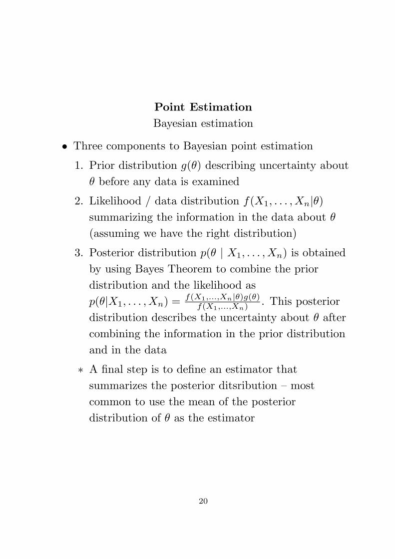
• Three components to Bayesian point estimation

1. Prior distribution g(θ) describing uncertainty aboutθ before any data is examined

2. Likelihood / data distribution f(X1, . . . , Xn|θ)summarizing the information in the data about θ

(assuming we have the right distribution)

3. Posterior distribution p(θ | X1, . . . , Xn) is obtainedby using Bayes Theorem to combine the priordistribution and the likelihood asp(θ|X1, . . . , Xn) = f(X1,...,Xn|θ)g(θ)

f(X1,...,Xn) . This posteriordistribution describes the uncertainty about θ aftercombining the information in the prior distributionand in the data

∗ A final step is to define an estimator thatsummarizes the posterior ditsribution – mostcommon to use the mean of the posteriordistribution of θ as the estimator

20


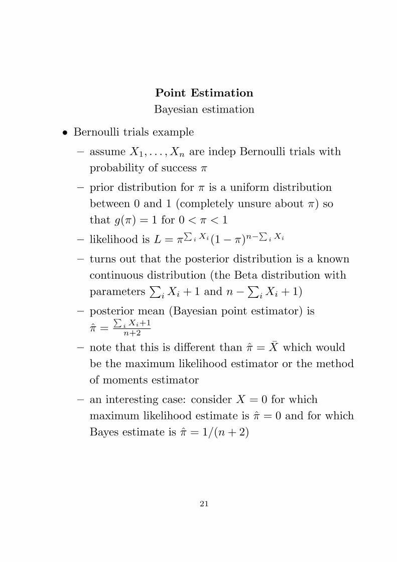
• Bernoulli trials example

– assume X1, . . . , Xn are indep Bernoulli trials withprobability of success π

– prior distribution for π is a uniform distributionbetween 0 and 1 (completely unsure about π) sothat g(π) = 1 for 0 < π < 1

– likelihood is L = π∑

i Xi(1− π)n−∑i Xi

– turns out that the posterior distribution is a knowncontinuous distribution (the Beta distribution withparameters

∑i Xi + 1 and n−∑

i Xi + 1)

– posterior mean (Bayesian point estimator) isπ =

∑i Xi+1

n+2

– note that this is different than π = X which wouldbe the maximum likelihood estimator or the methodof moments estimator

– an interesting case: consider X = 0 for whichmaximum likelihood estimate is π = 0 and for whichBayes estimate is π = 1/(n + 2)

21

Interval Estimation

• Point estimation is an important first step in astatistical problem

• A key contribution of the field of statistics though is tosupplement the point estimate with a measure ofaccuracy (e.g., the standard deviation of the estimatoris such a measure)

• A common way to convey the estimate and theaccuracy is through an interval estimate

• In other words we create an interval (based on thesample) which is likely to contain the true but unknownparameter value

• This interval is usually called a confidence interval (CI)

• There are a number of ways to create confidenceintervals, we focus on a simple approach appropriate forlarge samples to illustrate the approach

22

Central Limit Theorem

• A key mathematical result that enables intervalestimation (and other forms of statistical inference) isthe central limit theorem (CLT)

• Theorem: Let X1, . . . , Xn be a random sample of sizen from a distribution with mean µ and variance σ2.Then for large n, X = 1

n

∑i Xi is approximately normal

with mean µ and variance σ2/n.

• Note this means (X − µ)/(σ/√

n) is approximatelystandard normal

• How big does n have to be? It depends on thepopulation distribution

– if the population distribution is itself normal, thenthe CLT holds for small samples (even n = 1)

– if the population distribution is not too unusual,then the CLT holds for samples of 30 or more

– if the population distribution is unusual (e.g., verylong tails), then the CLT may require 100 or moreobservations

23

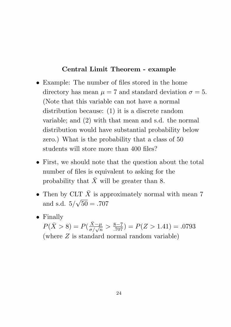
Central Limit Theorem - example

• Example: The number of files stored in the homedirectory has mean µ = 7 and standard deviation σ = 5.(Note that this variable can not have a normaldistribution because: (1) it is a discrete randomvariable; and (2) with that mean and s.d. the normaldistribution would have substantial probability belowzero.) What is the probability that a class of 50students will store more than 400 files?

• First, we should note that the question about the totalnumber of files is equivalent to asking for theprobability that X will be greater than 8.

• Then by CLT X is approximately normal with mean 7and s.d. 5/

√50 = .707

• FinallyP (X > 8) = P ( X−µ

σ/√

n> 8−7

.707 ) = P (Z > 1.41) = .0793(where Z is standard normal random variable)

24

Central Limit Theorem - binomial proportion

• You may recall that we saw a result something like theCLT in talking about the normal approximation to thebinomial distribution – if np > 5 and n(1− p) > 5 thenX ∼ Bin(n, p) can be approximated by a normalrandom variable Y having mean np and variancenp(1− p)

• This is equivalent to the CLT if we look at theproportion of successes X/n rather than the count ofsuccesses X

• To be specific, let W1, . . . , Wn be a random sample ofBernoulli trials (0/1 random variables) with probabilityof success p (hence mean is p and variance is p(1− p))and let X =

∑i Wi be the total number of successes in

n trials. Then by the CLT W = X/n is approximatelynormal with mean p and variance p(1− p)/n

25

Central Limit Theorem - binomial proportion

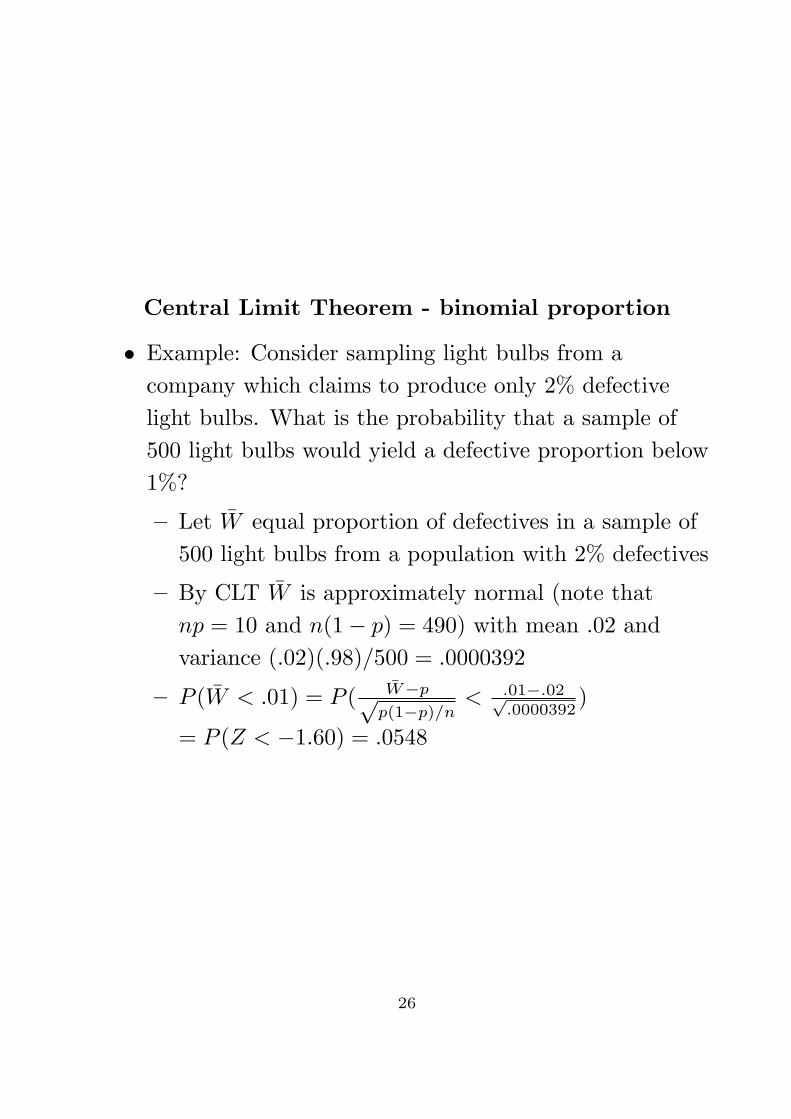
• Example: Consider sampling light bulbs from acompany which claims to produce only 2% defectivelight bulbs. What is the probability that a sample of500 light bulbs would yield a defective proportion below1%?

– Let W equal proportion of defectives in a sample of500 light bulbs from a population with 2% defectives

– By CLT W is approximately normal (note thatnp = 10 and n(1− p) = 490) with mean .02 andvariance (.02)(.98)/500 = .0000392

– P (W < .01) = P ( W−p√p(1−p)/n

< .01−.02√.0000392

)

= P (Z < −1.60) = .0548

26

Interval EstimationPopulation mean

• Central Limit Theorem enables us to easily build aconfidence interval for the mean of a population

• Assume X1, . . . , Xn are independent random variableswith mean µ and variance σ2

• Then X = 1n

∑i Xi (the sample mean) is the natural

estimate of µ (MLE, method of moments)

• We also know that X is a random variable which hasapproximately a normal distribution, X ∼ N(µ, σ2/n)

• It follows that Pr(−1.96 < X−µσ/√

n< 1.96) ≈ .95

• Thus X ± 1.96σ/√

n is an (approximate) 95%confidence interval for µ

• Note the above is an exact confidence interval if thepopulation distribution of the X’s is normal and anapproximate confidence interval valid for large n if not

27

Interval EstimationPopulation mean (cont’d)

• X ± 1.96σ/√

n is an (approximate) 95% confidenceinterval for µ (based on CLT)

• Some variations/improvements

– Different confidence level∗ We can get a different confidence level by using a

suitable percentile of the standard normaldistribution

∗ e.g., X ± 1.645σ/√

n is an (approximate) 90%confidence interval for µ

– Unknown population standard deviation∗ Results given so far require knowing the

population standard deviation σ

∗ If σ is not known (it usually isn’t) then we can usethe sample standard deviations =

√1

n−1

∑i(Xi − X)2 as an estimate

∗ Then X ± 1.96s/√

n is an approximate 95%confidence interval that should be good in largesamples (now even larger than before .. say 100observations or more)

∗ It turns out that it is possible to create a moreexact 95% confidence interval in this case byreplacing 1.96 with the relevant percentile ofStudent’s t-distribution (not covered in this class)

28

Interval EstimationBinomial proportion

• Assume X1, . . . , Xn are independent Bernoulli trialswith probability of success π (change from p now)

• Then π = 1n

∑i Xi = the sample proportion of successes

is the natural estimate (MLE, method of moments)

• From central limit theorem we know that π isapproximately normal with mean π and s.d.√

π(1− π)/n

• It follows that Pr(−1.96 < π−π√π(1−π)/n

< 1.96) = .95

• Thus any π for which the inequality above is satisfied isin a 95% confidence interval

• An alternative is replace the s.d. of π by an estimate,√π(1− π)/n and then note that π ± 1.96

√π(1− π)/n

is an approximate 95% confidence interval for π

29

Interval Estimation

• General approach

– the previous two examples suggest a generalapproach

– suppose that we have a point estimator θ for aparameter θ

– θ is a random variable with expected value typicallyapproximately equal to θ and with a standarddeviation s.d.(θ)

– it follows that an approximate large-sample 95%confidence interval for θ is given by θ ± 1.96 s.d.(θ)(sometimes we may need to estimate the s.d.)

• Interpretation

– it is important to remember the interpretation ofthese confidence intervals

– the “confidence” belongs to the procedure; we have aprocedure that creates intervals having the propertythat 95% of the confidence intervals contain the truevalues

– for any given instance the CI either contains thetrue value or not; our guarantee is only for averagebehavior in repeated samples

30

Tests/Decisions

• Point estimates and interval estimates are importantcomponents of statistical inference

• Sometimes there is a desire however for a formal test ordecision based on the value of a particular parameter

• For example:

– We may want to assess whether π = 0.5 in abinomial situation (or in other words we may wantto ask if we have a fair coin)?

– We may want to test whether µ = 0 (no change dueto an intervention)?

– We may want to compare average response in twogroups to see if they are equal (µ1 = µ2)?

31

Statistical Tests - binomial case

• We illustrate the basic approach in the binomial setting

• Assume we sample n people at random from list of CSfaculty in the U.S.

• Ask each whether their laptop runs Windows or Linux

• Observe 56% use Linux

• Can we conclude that a majority of CS faculty in theUS prefer Linux for their laptop?

– seems obvious that we can but ...

– the difference between 56% and 50% may just be afluke of the sample, the truth may be that thepopulation is split 50/50

32


• The logic of statistical tests

– let X denote the number of faculty preferring Linux

– assume X ∼ Bin(n, π)(note we use π instead of the usual p to avoidconfusion later)

– organize test in terms of null hypothesis (no effect,no difference) and alternative hypothesis (thedifference we suspect may be present)

∗ null Ho : π = 0.50∗ alternative Ha : π > 0.50∗ why use this formulation? easier to disprove

things statistically than to prove them

– we suspect Ho is false (and Ha is true) if X/n = π isgreater than 0.5. How much greater does it have tobe?

– approach: assume the null hypothesis is true and askwhether the observed data is as expected or isunusual

33

Statistical Tests - general comments

• There are two slightly different (but related) approaches

– significance tests – assess the evidence against Ho

with a p-value that measures how unusual theobserved data are

– hypothesis tests – formally establish a decisionrule for deciding between Ho and Ha to achievedesired goals (e.g., decide Ha is true if π > c where c

is chosen to control the probability of an error)

– we focus on significance tests in this class

34

Statistical Tests - general comments

• The key concept in significance tests is the p-value

• p-value = probability of observing data as or moreextreme than the data we obtained if Ho is true

• Low p-values are evidence that either(1) Ho is true and we saw an unusual eventor(2) Ho is not true

• The lower the p-value the more likely we are toconclude that Ho is not true

• Often use p < .05 as serious evidence against Ho but astrict cutoff is a BAD IDEA

• A couple of important points

– the p-value DOES NOT measure the probabilitythat Ho is true

– even if p-value is small the observed failure of Ho

may not be practically important

35


• Now return to binomial case and suppose that we havesampled 100 professors and find 56 use Linux, or inother words n = 100 and π = .56

• There are actually two ways to find the p-value: use thebinomial distribution directly or, if n is large (as it ishere) then we can use the CLT

• By the binomial distn ... let X be number of Linuxsupporters. Then under Ho we know X ∼ Bin(100, .5)and P (X ≥ 56) = .136 (not in our table but can becomputed)

• By the CLT ...

p-value = Pr(π ≥ 0.56 | π = 0.5)

= Pr(π − 0.50√.5(.5)/100

≥ .56− .50√.5(.5)/100

)

≈ Pr(Z ≥ 1.2) = .115

(using the continuity correction we’d sayp = P (π ≥ .555) = .136)

• Conclude: observed proportion .56 is higher thanexpected but could have happened by chance so can’tconclude that there is a significant preference for Linux

36


• Interpreting results

– The p-value of .136 does not mean that Ho is true, itonly means the current evidence is not strongenough to make us give it up

– p-value depends alot on sample size... with n = 200 and π = .56 we would have p = .045... with n = 400 and π = .56 we would have p = .008

37

Hypothesis Tests

• Significance tests focus on Ho and try to judge itsappropriateness

• Hypothesis tests treat the two hypotheses more evenlyand are thus used in more formal decision settings

– hypothesis testing procedures trade off two types oferrors

– type I error = reject Ho if it is true

– type II error = accept Ho if it is false

– we can vary cutoff of test; if we increase cutoff tomake it harder to reject Ho then we reduce type Ierrors but make more type II errors (and vice versaif we lower the cutoff)

• In practice hypothesis tests are very closely related tosignificance tests

38

Relationship of tests to other procedures

• Tests and confidence intervals

– confidence intervals provide a range of plausiblevalues for a parameter

– tests ask whether a specific parameter value seemsplausible

– these ideas are related ... suppose we have a 95%confidence interval for π

∗ if π = 0.50 is not in the confidence interval thenour test will tend to reject the hypothesis thatπ = 0.50

• Tests and Bayesian inference

– we have not emphasized the Bayesian approach totesting but there is one

– to see how it might work, recall that the Bayesianapproach yields a posterior distribution telling us,for example, the plausible values of π and how likelyeach is

– the Bayesian posterior distribution can computethings like P (π > 0.5|observed data) which seems todirectly address what we want to know

39

Decisions/Tests – general approach

• General setting: we have a hypothesis about aparameter θ, say Ho : θ = θo (could be π in binomial orµ in normal) and want to evaluate this null hypothesisagainst a suspected alternative Ha : θ > θo

• A general approach:

– obtain a suitable point estimate θ and use it to testthe hypothesis (reject Ho if θ is far from θo)

– calculate p-value which is P (θ > observed value)assuming Ho is true

– this calculation requires distribution of θ

– distribution of θ will depend on specific example(e.g., binomial case above)

• Of course if alternative is θ < θo then p-value also uses“<”

40

Decisions/Test – population mean

Example: Tests for µ (the population mean)

• Natural estimate is X (the sample mean)

• What do we know about the distribution of X underHo?

– If the population data are normal and σ is known,then X is normal with mean µo and s.d. σ/

√n

– If the population data are normal and σ is notknown, then X is approximately normal with meanµo and s.d. s/

√n for large sample size

– If sample size is large (no matter what thepopulation data are), then X is approximatelynormal with mean µo and s.d. s/

√n

– Only difference between the last two items is thatmight expect to need a “larger” sample size in thelast case

• The above discussion leads to normal test ofHo : µ = µo withp-value = P (X > x) = P (Z > (x− µo)/ s√

n)

(with Z the usual standard normal distn)

41


Example: Tests for µ (the population mean)

Some technical stuff (optional)

• When we don’t know σ and plug in the estimate s, weshould really adjust for this in our procedure

• It turns out that the proper adjustment (originaldiscovered by a brewery worker!) is to use Student’st-distribution in place of the standard normaldistribution

• Student’s t-distribution is a distribution that lookssomething like the normal but has heavier tails (biggervalues are possible). The t distribution is described bythe number of degrees of freedom (how big a sample itis based on) with a large degrees of freedomcorresponding more closely to a normal distribution

• Student’s t-test of Ho : µ = µo would lead top-value = P (X > x) = P (Z > (x− µo)/ s√

n)

where tn−1 is a random variable having Student’st-distribution with n− 1 degrees of freedom

• For Stat 67 purposes ... just need to know that in largesamples can use normal table and not worry about theStudent’s t-distribution

42


• Numerical example:

Suppose that the average database query response timeis supposed to be 1 second or faster. We try 100 queriesand observe an average response time of 1.05 seconds(with a standard deviation of .25 seconds). Can weconclude that the database does not meet its standard?

– frame question as a statistical test:Ho : µ = 1 vs Ha : µ > 1

– p-value= P (Z ≥ (1.05− 1.00)/ .25√

100) = P (Z ≥ 2) = .023

(if we use Student’s t-test, then p-value = .024)

– reject Ho and conclude that the database is notperforming as advertised

– note that the additional .05 seconds may not bepractically important

43

Decisions/Test – difference between two means

Note to self: If there is time, then do this slide and thenext to show how testing handles harder problems

• A common situation is that we have two populationsand we want to compare the means of the twopopulations

• Example (medical): suppose we have two treatments(drug A and drug B) and wish to compare averagesurvival time of cancer patients given drug A (µ1) toaverage survival time of cancer patients given drug B(µ2)

• Assuming we have data on the two populations

– Y1 − Y2 is an estimator for µ1 − µ2

– y1 − y2 is an estimate for µ1 − µ2

– Var(Y1 − Y2) = σ2(

1n1

+ 1n2

)

– S2p = (n1−1)S2

1+(n2−1)S22

n1+n2−2 is a pooledestimator for common variance σ2

• Key result: under assumptions

t =Y1 − Y2 − (µ1 − µ2)

Sp

√1

n1+ 1

n2

∼ tn1+n2−2

• Again for Stat 67 don’t worry about Student’s t (forlarge samples can use normal distribution)

44

Decisions/Test – difference between two means

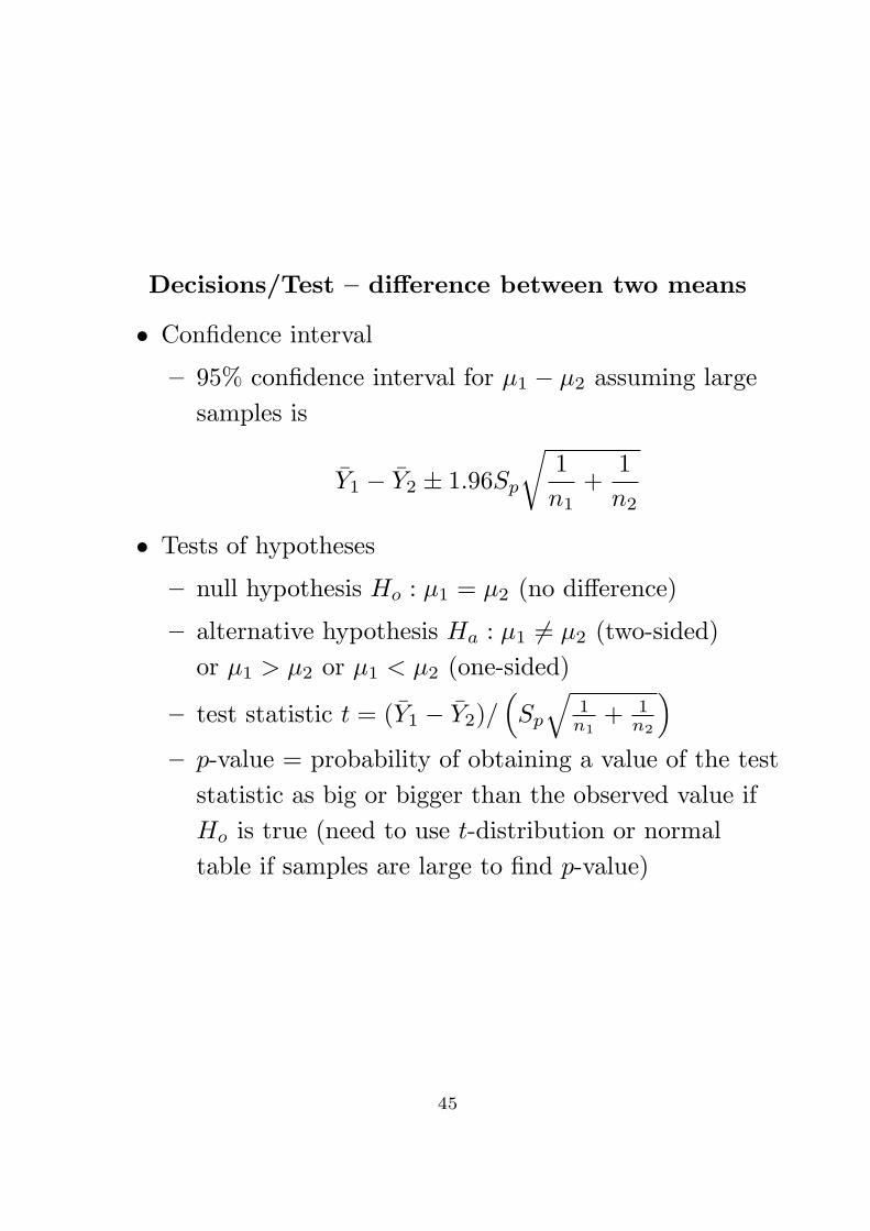
• Confidence interval

– 95% confidence interval for µ1 − µ2 assuming largesamples is

Y1 − Y2 ± 1.96Sp

√1n1

+1n2

• Tests of hypotheses

– null hypothesis Ho : µ1 = µ2 (no difference)

– alternative hypothesis Ha : µ1 6= µ2 (two-sided)or µ1 > µ2 or µ1 < µ2 (one-sided)

– test statistic t = (Y1 − Y2)/(Sp

√1

n1+ 1

n2

)

– p-value = probability of obtaining a value of the teststatistic as big or bigger than the observed value ifHo is true (need to use t-distribution or normaltable if samples are large to find p-value)

45

Probability and Statistical Modeling

• So far:

– Estimation∗ sample from population with assumed distribution∗ inference for mean or variance or other parameter∗ point or interval estimates

– Decisions / Tests

∗ judge whether data are consistent with assumedpopulation

∗ judge whether two populations have equal means

– To apply statistical thinking in more complexsettings (e.g., machine learning)∗ build a probability model relating observable data

to underlying model parameters∗ use statistical methods to estimate parameters

and judge fit of model

46

Simple linear regressionIntroduction

• We use linear regression as a (relatively simple)example of statistical modeling

• Linear regression refers to a particular approach forstudying the relationship of two or more quantitativevariables variables

• Examples:

– predict salary from education, years ofexperience, age

– find effect of lead exposure on schoolperformance

• Useful to distinguish between a functional ormathematical model

Y = g(X) (deterministic)and a structural or statistical model

Y = g(X)+error (stochastic)

47

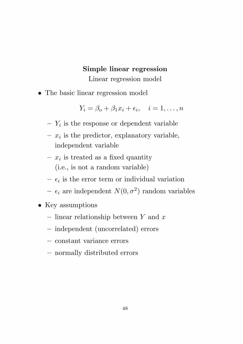
Simple linear regressionLinear regression model

• The basic linear regression model

Yi = βo + β1xi + εi, i = 1, . . . , n

– Yi is the response or dependent variable

– xi is the predictor, explanatory variable,independent variable

– xi is treated as a fixed quantity(i.e., is not a random variable)

– εi is the error term or individual variation

– εi are independent N(0, σ2) random variables

• Key assumptions

– linear relationship between Y and x

– independent (uncorrelated) errors

– constant variance errors

– normally distributed errors

48

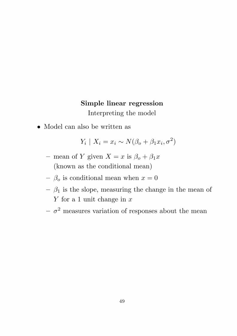
Simple linear regressionInterpreting the model

• Model can also be written as

Yi | Xi = xi ∼ N(βo + β1xi, σ2)

– mean of Y given X = x is βo + β1x

(known as the conditional mean)

– βo is conditional mean when x = 0

– β1 is the slope, measuring the change in the mean ofY for a 1 unit change in x

– σ2 measures variation of responses about the mean

49

Simple linear regressionWhere does this model come from?

• This model may be plausible based on a physical orother argument

• The model may just be a convenient approximation

• One special case is worth mentioning:It turns out that if we believe that two randomvariables X and Y have a bivariate normal distribution(remember we saw this briefly), then the conditionaldistribution of Y given X is in fact a normal modelwith mean equal to a linear function of X and constantvariance

50

Simple linear regressionEstimation

• Maximum likelihood estimation

– we can write down joint distn of all of the Y ’s,known as the likelihood function

L(βo, β1, σ2 | Y1, . . . , Yn) =

n∏

i=1

N(Yi | βo + β1xi, σ2)

– we maximize this to get estimates βo, β1

– turns out to be equivalent to ....

• Least squares estimation

– choose βo, β1 to minimizeg(βo, β1) =

∑ni=1(Yi − (βo + β1xi))2

– least squares has a long history (even withoutassuming a normal distribution)∗ why squared errors? (convenient math)∗ why vertical distances? (Y is response)

– result:

βo = Y − β1x

β1 =∑n

i=1(xi − x)(Yi − Y )∑ni=1(xi − x)2

– predicted (or fitted) value for a case with X = xi isYi = βo + β1xi

– residual (or error) is ei = Yi − Yi

51

Simple linear regressionEstimation - some details

• Least squares estimation:choose βo, β1 to minimize

g(βo, β1) =n∑

i=1

(Yi − (βo + β1xi))2

• Taking derivatives and setting them equal to zero yieldsnormal equations

βon + β1

∑xi =

∑Yi

βo

∑xi + β1

∑x2

i =∑

xiYi

• Solving these equations leads to answers on previousslide

52

Simple linear regressionEstimation of error variance

• Maximum likelihood estimate of σ2 is1n

∑i(Yi − Yi)2 = 1

n

∑i e2

i

• It turns out that this estimate is generally too small

• A common estimate of σ2 is

s2e =

1n− 2

n∑

i=1

(Yi − (βo + β1xi))2 =1

n− 2

n∑

i=1

e2i

which is used because the 1n−2 makes this an unbiased

estimate

53

Simple linear regressionInference for β1

• There are many quantities of interest in a regressionanalysis

• We may be interested in learning about

– the slope β1

– the intercept βo

– a particular fitted value βo + β1x

– a prediction for an individual

• Time is limited so we discuss only drawing statisticalconclusions about the slope

54

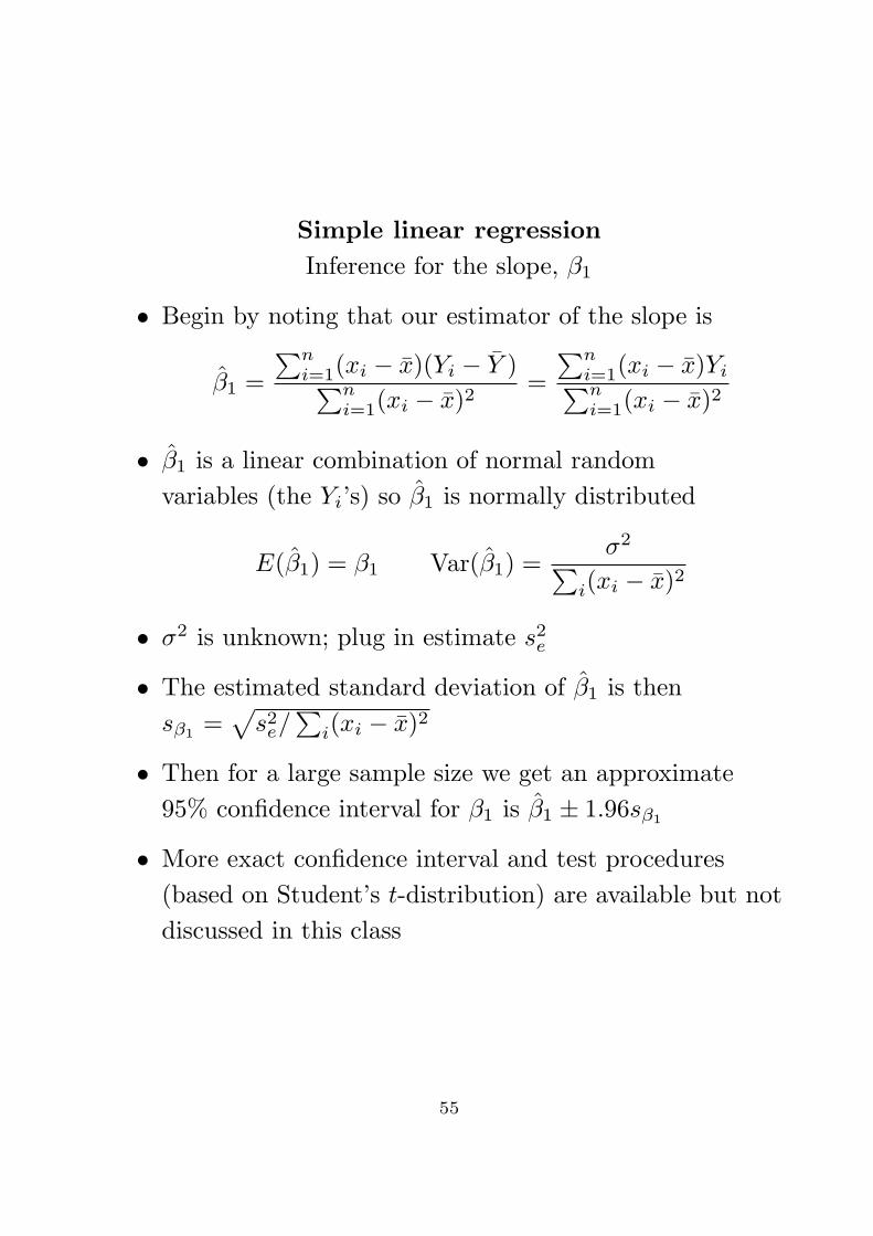
Simple linear regressionInference for the slope, β1

• Begin by noting that our estimator of the slope is

β1 =∑n

i=1(xi − x)(Yi − Y )∑ni=1(xi − x)2

=∑n

i=1(xi − x)Yi∑ni=1(xi − x)2

• β1 is a linear combination of normal randomvariables (the Yi’s) so β1 is normally distributed

E(β1) = β1 Var(β1) =σ2

∑i(xi − x)2

• σ2 is unknown; plug in estimate s2e

• The estimated standard deviation of β1 is thensβ1 =

√s2

e/∑

i(xi − x)2

• Then for a large sample size we get an approximate95% confidence interval for β1 is β1 ± 1.96sβ1

• More exact confidence interval and test procedures(based on Student’s t-distribution) are available but notdiscussed in this class

55

Simple linear regressionModel diagnostics - residuals

• We can check whether the linear regression model is asensible model using the residuals

• Recall ei = Yi − Yi = Yi − βo − β1xi

• ei is an approximation of the stochastic error (εi) in ourmodel

• Important properties

– sum of residuals is zero hence a typical value is zero

– variance of the residuals is approximately equal toone

– if our model is correct the residuals should looksomething like a N(0, 1) sample

– we can look to see if there are patterns in theresiduals that argue against our model

56

Simple linear regressionDiagnosing violations with residual plots

• Plot residuals versus predicted values and look forpatterns

– might detect nonconstant variance

– might detect nonlinearity

– might detect outliers

• Histogram or other display of residuals

– might detect nonnormality

• Show sample pictures in class

57

Simple linear regressionRemedies for violated assumptions

• What if we find a problem?

• Sometimes the linear regression model will work with a“fix”

– transform Y (use log Y or√

Y as the response)

– add or modify predictors (perhaps add X2 toapproximate a quadratic relationship)

• If no easy “fix”, then we can consider moresophisticated models

58

Documents

Statistics 67 Introduction to Probability and Statistics ...sternh/courses/67/stat67slides.pdf · Introduction to Probability and Statistics for Computer Science Lecture notes for