Statistical unfolding of elementary particle spectra: …smat.epfl.ch/victor/papers/KuuselaPanaretos_AOAS2015.pdf · 2015-11-03 · STATISTICAL UNFOLDING OF ELEMENTARY PARTICLE SPECTRA:

The Annals of Applied Statistics2015, Vol. 9, No. 3, 1671–1705DOI: 10.1214/15-AOAS857© Institute of Mathematical Statistics, 2015

STATISTICAL UNFOLDING OF ELEMENTARY PARTICLESPECTRA: EMPIRICAL BAYES ESTIMATION AND

BIAS-CORRECTED UNCERTAINTY QUANTIFICATION

BY MIKAEL KUUSELA1,2 AND VICTOR M. PANARETOS1

École Polytechnique Fédérale de Lausanne

We consider the high energy physics unfolding problem where the goalis to estimate the spectrum of elementary particles given observations dis-torted by the limited resolution of a particle detector. This important statisti-cal inverse problem arising in data analysis at the Large Hadron Collider atCERN consists in estimating the intensity function of an indirectly observedPoisson point process. Unfolding typically proceeds in two steps: one firstproduces a regularized point estimate of the unknown intensity and then usesthe variability of this estimator to form frequentist confidence intervals thatquantify the uncertainty of the solution. In this paper, we propose forming thepoint estimate using empirical Bayes estimation which enables a data-drivenchoice of the regularization strength through marginal maximum likelihoodestimation. Observing that neither Bayesian credible intervals nor standardbootstrap confidence intervals succeed in achieving good frequentist cover-age in this problem due to the inherent bias of the regularized point estimate,we introduce an iteratively bias-corrected bootstrap technique for construct-ing improved confidence intervals. We show using simulations that this en-ables us to achieve nearly nominal frequentist coverage with only a modestincrease in interval length. The proposed methodology is applied to unfoldingthe Z boson invariant mass spectrum as measured in the CMS experiment atthe Large Hadron Collider.

1. Introduction. This paper studies a generalized linear inverse problem[Bochkina (2013)], called the unfolding problem [Blobel (2013), Cowan (1998),Prosper and Lyons (2011)], arising in data analysis at the Large Hadron Collider(LHC) at CERN, the European Organization for Nuclear Research. The LHC isthe world’s largest and most powerful particle accelerator. It collides two beamsof protons in order to study the properties and interactions of elementary parti-cles produced in such collisions. The trajectories and energies of these particlesare recorded using gigantic underground particle detectors and the vast amountsof data produced by these experiments are analyzed in order to draw conclusions

Received January 2014; revised July 2015.1Supported in part by a Swiss National Science Foundation grant.2Supported in part by a grant from the Helsinki Institute of Physics.Key words and phrases. Poisson inverse problem, high energy physics, Large Hadron Collider,

Poisson process, regularization, bootstrap, Monte Carlo EM Algorithm.

1671

http://www.imstat.org/aoas/

http://dx.doi.org/10.1214/15-AOAS857

http://www.imstat.org

1672 M. KUUSELA AND V. M. PANARETOS

about fundamental laws of physics. Due to their complex structure and huge quan-tity, the analysis of these data poses significant statistical and computational chal-lenges.

Experimental high energy physicists use the term “unfolding” to refer to correct-ing the distributions measured at the LHC for the limited resolution of the particledetectors. Let X be some physical quantity of interest measured in the detector.This could, for example, be the energy, mass or production angle of a particle. Dueto the noise induced by the detector, we are only able to observe a stochasticallysmeared or folded version Y of this quantity. As a result, the observed distributionof Y is a “blurred” version of the true, physical distribution of X and the task is touse the observed values of Y to estimate the distribution of X. Each year, the exper-imental collaborations working with LHC data produce dozens of physics resultsthat make use of unfolding. Recent examples include studies of the characteris-tics of jets [Chatrchyan et al. (2012a)], the transverse momentum distribution ofW bosons [Aad et al. (2012)] and charge asymmetry in top-quark pair production[Chatrchyan et al. (2012b)], to name a few.

The main challenge in unfolding is the ill-posedness of the problem in the sensethat a simple inversion of the forward mapping from the true space into the smearedspace is unstable with respect to small perturbations of the data [Engl, Hanke andNeubauer (2000), Kaipio and Somersalo (2005), Panaretos (2011)]. As such, thetrivial maximum likelihood solution of the problem often exhibits spurious high-frequency oscillations. These oscillations can be tamed by regularizing the prob-lem, which is done by taking advantage of additional a priori knowledge aboutplausible solutions.

An additional complication is the non-Gaussianity of the data which followsfrom the fact that both the true and the smeared observations are realizations oftwo interrelated Poisson point processes, which we denote by M and N , respec-tively. As such, unfolding is an example of a Poisson inverse problem [Antoniadisand Bigot (2006), Reiss (1993)], where the intensity function f of the true processM is related to the intensity function g of the smeared process N via a Fredholmintegral operator K , that is, g = Kf , where K represent the response of the detec-tor. The task at hand is then to estimate and make inferences about the true intensityf given a single observation of the smeared process N . Due to the Poisson natureof the data, many standard techniques based on a Gaussian likelihood function,such as Tikhonov regularization, are only approximately valid for unfolding. Fur-thermore, estimators properly taking into account the Poisson distribution of theobservations are rarely available in a closed form, making the problem computa-tionally challenging.

At present, the unfolding methodology used in LHC data analysis is notwell established [Lyons (2011)]. The two main approaches are the expectation–maximization (EM) algorithm with an early stopping [D’Agostini (1995), Lucy(1974), Richardson (1972), Vardi, Shepp and Kaufman (1985)] and a certain vari-ant of Tikhonov regularization [Höcker and Kartvelishvili (1996)]. In high en-ergy physics (HEP) terminology, the former is called the D’Agostini iteration and

STATISTICAL UNFOLDING OF ELEMENTARY PARTICLE SPECTRA 1673

the latter, somewhat misleadingly, SVD unfolding (with SVD referring to the sin-gular value decomposition). In addition, a HEP-specific heuristic, called bin-by-bin unfolding, which provably accounts for smearing effects incorrectly through amultiplicative efficiency correction, has been widely used. Recently, Choudalakis(2012) proposed a Bayesian solution to the problem, but this seems to have seldombeen used in practice thus far.

The main problem with the D’Agostini iteration is that it is difficult to give aphysical interpretation to the regularization imposed by early stopping of the itera-tion. SVD unfolding, on the other hand, ignores the Poisson nature of the observa-tions and does not enforce the positivity of the solution. Furthermore, both of thesemethods suffer from not dealing with two significant issues satisfactorily: (1) thechoice of the regularization strength and (2) quantification of the uncertainty of thesolution. The delicate problem of choosing the regularization strength is handledin most LHC analyses using nonstandard heuristics or, in the worst-case scenario,by simply fixing some value “by hand.” When quantifying the uncertainty of theunfolded spectrum, the analysts form approximate frequentist confidence intervalsusing simple error propagation, but little is known about the coverage propertiesof these intervals.

In this paper, we propose new statistical methodology aimed at addressing thetwo above-mentioned issues in a more satisfactory manner. Our main methodolog-ical contributions are as follows:

1. Empirical Bayes selection of the regularization parameter using a MonteCarlo expectation–maximization algorithm [Casella (2001), Geman and McClure(1985, 1987), Saquib, Bouman and Sauer (1998)];

2. Frequentist uncertainty quantification using a combination of an iterativebias-correction procedure [Goldstein (1996), Kuk (1995)] and bootstrap percentileintervals [Davison and Hinkley (1997), Efron and Tibshirani (1993)].

To the best of our knowledge, neither of these techniques has been previously usedto solve the HEP unfolding problem. Our framework also properly takes into ac-count the Poisson distribution of the observations, enforces the positivity constraintof the unfolded spectrum and imposes a curvature penalty on the solution with aclear physical interpretation.

It is helpful to think of the unfolding problem as consisting of two separate, butrelated, subproblems: one of point estimation and the other of uncertainty quantifi-cation. We follow the standard practice of first constructing a point estimate of theunknown intensity and then using the variability of this point estimate to form fre-quentist confidence intervals. For the point estimation part, the main challenge is todecide how to regularize the ill-posed problem and, in particular, how to choose theregularization strength. Classical, well-known techniques for making this choiceinclude the Morozov discrepancy principle [Morozov (1966)] and cross-validation[Stone (1974)]. Bardsley and Goldes (2009) study these techniques in the context


of Poisson inverse problems, while Veklerov and Llacer (1987) provide an alterna-tive approach based on statistical hypothesis testing. From a Bayesian perspective,the problem can be addressed using a Bayesian hierarchical model [Kaipio andSomersalo (2005)] which necessitates the choice of a hyperprior for the regular-ization parameter. On the other hand, empirical Bayes selection of the regulariza-tion parameter using the marginal likelihood, which has the key advantage of notrequiring the specification of a hyperprior, has received relatively less attention inthe inverse problems literature. However, in many other fields of statistical infer-ence, such as semiparametric regression [Ruppert, Wand and Carroll (2003), Wood(2011), Section 5.2], neural networks [Bishop (2006), Sections 3.5 and 5.7.2] andGaussian processes [Rasmussen and Williams (2006), Chapter 5], the use of em-pirical Bayes techniques has become part of standard practice. The approach wefollow bears similarities to that of Saquib, Bouman and Sauer (1998), where themarginal maximum likelihood estimator is used to select the regularization param-eter in tomographic image reconstruction with Poisson data.

Once we have formed an empirical Bayes point estimate of the unknown in-tensity function, we would like to use the variability of this point estimator toquantify the uncertainty of the solution. In high energy physics, frequentist confi-dence statements are generally preferred over Bayesian alternatives [Lyons (2013)]and we would hence like to obtain confidence intervals with good frequentist cov-erage properties. To achieve this, the main challenge comes from the bias that ispresent in the point estimate in order to regularize the otherwise ill-posed prob-lem. We show using simulations that this bias can seriously degrade the cover-age probability of both Bayesian credible intervals and standard bootstrap con-fidence intervals. We propose to remedy this problem by employing an itera-tive bias-correction technique [Goldstein (1996), Kuk (1995)] and then using thevariability of the bias-corrected point estimate to form the confidence intervals.Quite remarkably, our simulation results indicate that such a technique achievesclose-to-nominal coverage with only a modest increase in the length of the inter-vals.

The paper is structured as follows. Section 2 gives a brief overview of the LHCdetectors and explains the role that unfolding plays in these experiments. We thenformulate in Section 3 a forward model for the unfolding problem using Poissonpoint processes. The proposed statistical methodology is explained in detail inSection 4 which forms the backbone of this paper. This is followed by simulationstudies in Section 5 and a real-world data analysis scenario in Section 6 whichconsists of unfolding of the Z boson invariant mass spectrum measured in theCMS experiment at the LHC. We close the paper with some concluding remarks inSection 7. We also invite the reader to consult the online supplement [Kuusela andPanaretos (2015)] which provides further simulation results and some technicaldetails.


2. LHC experiments and unfolding.

2.1. Overview of LHC experiments. The Large Hadron Collider is a 27 kmlong circular proton–proton collider located in an underground tunnel at CERNin Geneva, Switzerland. With proton–proton collisions of up to 13 TeV3 center-of-mass energy, the LHC is the world’s most powerful particle accelerator. Theprotons are accelerated in bunches of billions of particles and bunches moving inopposite directions are led to collide at the center of four gigantic particle detectorscalled ALICE, ATLAS, CMS and LHCb. In the LHC Run 1 configuration, thesebunches collided every 50 ns at the heart of the detectors, resulting in some 20million collisions per second in each detector, out of which the few hundred mostinteresting ones were stored for further analysis. In LHC Run 2, which started inJune 2015, the collision rate is likely to be even higher.

Out of the four detectors, ATLAS and CMS are multipurpose experiments capa-ble of performing a large variety of physics analyses ranging from the discovery ofthe Higgs boson to precision studies of quantum chromodynamics. The other twodetectors, ALICE and LHCb, specialize in studies of lead-ion collisions and b-hadrons, respectively. In what follows, we focus on describing the data collectionand analysis in the CMS experiment, which is also the source of the data of ourunfolding demonstration in Section 6, but similar principles also apply to ATLASand, to some extent, to other high energy physics experiments.

The CMS experiment [Chatrchyan et al. (2008)], an acronym for CompactMuon Solenoid, is situated in an underground cavern along the LHC ring nearthe village of Cessy, France. The detector, weighing a total of 12,500 tons, has acylindrical shape with a diameter of 14.6 m and a length of 21.6 m. The construc-tion, operation and data analysis of the experiment is conducted by an internationalcollaboration of over 4000 scientists, engineers and technicians. When two protonscollide at the center of CMS, their energy is transformed into matter in the form ofnew particles. A small fraction of these particles are exotic, short-lived particles,such as the Higgs boson or the top quark, which are at the center of the scientific in-terest of the high energy physics community. Such particles decay almost instantlyinto more familiar, stable particles, such as electrons, muons or photons. Usingvarious subdetectors, the energies and trajectories of these particles are recordedin order to study the properties and interactions of the exotic particles created inthe collision.

The layout of the CMS detector is illustrated in Figure 1. The detector is im-mersed in a 3.8 T magnetic field created using a superconducting solenoid magnet.This magnetic field bends the trajectory of any charged particle traversing the de-tector. This enables the measurement of the particle’s momentum, since the higherthe momentum, the less the particle’s trajectory is bent.

3The electron volt, eV, is the customary unit of energy used in particle physics, 1 eV ≈ 1.6 ·10−19 J.


FIG. 1. Illustration of the detection of particles at the CMS experiment [Barney (2004)]. Each typeof particle leaves its characteristic trace in the various subdetectors of the experiment. This enablesidentification of different particles as well as the measurement of their energies and trajectories.Copyright: CERN, for the benefit of the CMS Collaboration.

CMS consists of three layers of subdetectors: the tracker, the calorimeters andthe muon detectors. The innermost detector is the silicon tracker, which consists ofan inner layer of pixel detectors and an outer layer of microstrip detectors. Whena charged particle passes through these semiconducting detectors, it leaves behindelectron–hole pairs, and hence creates an electric signal. These signals are com-bined into a particle track using a Kalman filter in order to reconstruct the trajectoryof the particle.

The next layer of detectors are the calorimeters, which are devices for mea-suring the energies of particles. The CMS calorimeter system is divided into anelectromagnetic calorimeter (ECAL) and a hadron calorimeter (HCAL). Both ofthese devices are based on the same general principle: they are made of extremelydense materials with the aim of stopping the particles passing through. In the pro-cess, a portion of the energy of these particles is converted into light in a scin-tillating material and the amount of light, which depends on the energy of theincoming particle, is measured using photodetectors inside the calorimeters. TheECAL measures the energy of particles that interact mostly via the electromag-netic interaction, in other words, electrons, positrons and photons. The HCAL, onthe other hand, measures the energies of hadrons, that is, particles composed ofquarks. These include, for example, protons, neutrons and pions. The HCAL isalso instrumental in measuring the energies of jets, that is, collimated streams ofhadrons produced by quarks and gluons, and in detecting the so-called missingtransverse energy, an energy imbalance caused by noninteracting particles, such asneutrinos, escaping the detector.


The outermost layer of CMS consists of muon detectors, whose task is to iden-tify muons and measure their momenta. Accurate detection of muons was of cen-tral importance in the design of CMS since muons provide a clean signature formany exciting physics processes. This is because there is a very low probability forother particles, with the exception of noninteracting neutrinos, to penetrate throughthe CMS calorimeter system. For example, the four-muon decay channel playedan important role in the discovery of the Higgs boson at CMS [Chatrchyan et al.(2012c)].

The information of all CMS subdetectors is combined [Chatrchyan et al. (2009)]to identify the stable particles, that is, muons, electrons, positrons, photons andvarious types of hadrons, produced in each collision event; see Figure 1. For ex-ample, a muon will leave a track in both the silicon tracker and the muon chamber,while a photon produces a signal in the ECAL without an associated track in thetracker. The information of these individual particles is then used to reconstructhigher-level physics objects, such as jets or missing transverse energy.

2.2. Unfolding in LHC data analysis. The need for unfolding arises becauseany quantity measured at the LHC detectors is corrupted by stochastic noise. Forexample, let E be the true energy of an electron hitting the CMS ECAL. Thenthe observed value of the energy follows to a good approximation the Gaussiandistribution N (E, σ 2(E)), where the variance satisfies [Chatrchyan et al. (2008)]

(σ(E)

E

)2

=(

S√E

)2

+(

N

E

)2

+ C2,(1)

where S, N and C are fixed constants. The measurement noise is not always addi-tive. Furthermore, for more sophisticated measurements, such as the ones combin-ing information from several subdetectors or more than one particle, the distribu-tion of the response is usually not available in a closed form. Indeed, most analysesrely on detector simulations or auxiliary measurements to determine the detectorresponse.

It should be pointed out that not all LHC physics analyses directly rely on un-folding. The common factor between the examples given in Section 1 is that theseare measurement analyses and not discovery analyses, meaning that these are anal-yses studying in detail the properties of some already known phenomenon. In sucha case, the experimental interest often lies in the detailed particle-level shape ofsome distribution which can be obtained using unfolding, while discovery analy-ses are almost exclusively carried out in the smeared space. Unfolding neverthelessplays an indirect role in attempts to discover new physics at the LHC. Namely, dis-covery analyses often use unfolded results as inputs to their analysis chain.

The need to unfold the measurements usually arises for the purposes of thefollowing:


• Comparison of experiments with different responses: The only direct way ofcomparing the spectra measured in two different experiments is to compare theunfolded measurements.

• Input to a subsequent analysis: Certain tasks, such as the estimation of partondistributions functions or the fine-tuning of Monte Carlo event generators, typi-cally require unfolded input spectra.

• Comparison with future theories: When unfolded spectra are published, the-orists can directly use them to compare with any new theoretical predictionswhich might not have existed at the time of the original measurement. This jus-tification is sometimes considered controversial since, alternatively, one couldpublish the response of the detector and the theorists could use it to smear theirnew predictions.

• Exploratory data analysis: The unfolded spectrum could reveal hidden featuresand structure in the data which are not considered in any of the existing theoret-ical predictions.

According to the CERN Document Server (https://cds.cern.ch/), the CMS ex-periment published in 2012 a total of 103 papers out of which 16 made direct useof unfolding and many more indirectly relied on unfolded results. That year, un-folding was most often used in studies of quantum chromodynamics (4 papers),forward physics (4) and properties of the top quark (3). Most of these results reliedon the questionable bin-by-bin heuristic (8), while the EM algorithm (3) and var-ious forms of penalization (6) were also used. We expect similar statistics to alsohold for the other LHC experiments.

3. Problem formulation. In most situations in high energy physics, the datageneration mechanism can be modeled as a Poisson point process [see, e.g., Reiss(1993)]. Let E be a compact interval on R, f a nonnegative function in L2(E) andM a discrete random measure on E. Then M is a Poisson point process on statespace E with intensity function f if and only if:

1. M(B) ∼ Poisson(λ(B)) with λ(B) = ∫B f (s)ds for every Borel set B ⊂ E;

2. M(B1), . . . ,M(Bn) are independent for pairwise disjoint Borel sets Bi ⊂E, i = 1, . . . , n.

In other words, the number of points M(B) observed in the set B ⊂ E is Pois-son distributed with mean

∫B f (s)ds and the number of points in disjoint sets are

independent random variables.For the problem at hand, the Poisson process M represents the true, particle-

level spectrum of events. The smeared, detector-level spectrum is represented byanother Poisson process N . The process N is assumed to have a state space F ,which is a compact interval on R, and a nonnegative intensity function g ∈ L2(F ).The intensities of the two processes are related by a bounded linear operator K :

https://cds.cern.ch/


L2(E) → L2(F ) so that g = Kf . In what follows, we assume K to be a Fredholmintegral operator, that is,

g(t) = (Kf )(t) =∫E

k(t, s)f (s)ds,(2)

where the kernel k ∈ L2(F × E). For the purposes of this paper, we assume that k

is known, although in reality there is usually an uncertainty associated with it; seeSection 7. The unfolding problem is then to estimate the true intensity f given asingle observation of the smeared Poisson process N .

This Poisson inverse problem [Antoniadis and Bigot (2006), Reiss (1993)] isill-posed in the sense that in virtually all practical cases the pseudoinverse K† ofthe forward operator K is an unbounded, and hence discontinuous, linear operator[Engl, Hanke and Neubauer (2000)]. This means that the naïve approach of firstestimating g using, for example, a kernel density estimate g and then estimating f

using f = K†g is unstable with respect to fluctuations of g.To better understand the physical meaning of the kernel k, let us consider the

unfolding problem at the point level. Denoting by Xi the true observables, thePoisson point process M can be written as M = ∑τ

i=1 δXi, where δXi

is the Diracmeasure at Xi ∈ E and τ,X1,X2, . . . are independent random variables such thatτ ∼ Poisson(λ(E)) and the Xi are identically distributed with probability densityf (·)/λ(E), where λ(E) = ∫

E f (s)ds.When the particle corresponding to Xi traverses the detector, the first thing that

can happen is that it might not be observed at all due to the limited efficiency andacceptance of the device. Mathematically, this corresponds to thinning of the Pois-son process. Let Zi ∈ {0,1} be an indicator variable showing whether the point Xi

is observed (Zi = 1) or not (Zi = 0). We assume that τ, (X1,Z1), (X2,Z2), . . . areindependent and that the pairs (Xi,Zi) are identically distributed. Then the thinnedtrue process is given by M∗ = ∑τ

i=1 ZiδXi= ∑ξ

i=1 δX∗i, where ξ = ∑τ

i=1 Zi andthe X∗

i are the true points with Zi = 1. The thinned process M∗ is a Poisson pointprocess with intensity function f ∗(s) = ε(s)f (s), where ε(s) = P(Zi = 1|Xi = s)

is the efficiency of the detector for a true observation at s ∈ E.For each observed point X∗

i ∈ E, the detector measures a noisy value Yi ∈ F .We assume that the smeared observations Yi are i.i.d. with probability density

p(Yi = t) =∫E

p(Yi = t |X∗

i = s)p

(X∗

i = s)

ds.(3)

From this, it follows that the smeared observations Yi constitute a Poisson pointprocess N = ∑ξ

i=1 δYiwhose intensity function g is given by

g(t) =∫E

p(Yi = t |X∗

i = s)ε(s)f (s)ds.(4)

We hence identify that the kernel k in equation (2) is given by

k(t, s) = p(Yi = t |X∗

i = s)ε(s).(5)


Notice that in the special case where k(t, s) = k(t − s), unfolding becomes a de-convolution problem [Meister (2009)] for Poisson point process observations.

4. Unfolding methodology.

4.1. Outline of the proposed methodology. In this section we propose a novelcombination of statistical methods for solving the high energy physics unfoldingproblem formalized in Section 3. The proposed methodology is based on the fol-lowing key ingredients:

1. Discretization:(a) The smeared observations are discretized using a histogram.(b) The unknown particle-level intensity is modeled using a B-spline, that is,

f (s) = ∑pj=1 βjBj (s), s ∈ E, where Bj(s), j = 1, . . . , p, are the B-spline

basis functions.2. Point estimation:

(a) Posterior mean estimation of the unknown basis coefficients β = [β1, . . . ,

βp]T using a single-component Metropolis–Hastings sampler.(b) Empirical Bayes estimation of the scale δ of the regularizing smoothness

prior p(β|δ) using a Monte Carlo EM algorithm.3. Uncertainty quantification:

(a) Iterative bias-correction of the point estimate β .(b) Use of bootstrap percentile intervals of the bias-corrected intensity function

to form pointwise frequentist confidence bands for f .

This methodology enables a principled solution of the unfolding problem, in-cluding the choice of the regularization strength and frequentist uncertainty quan-tification. We explain below each of these steps in detail and argue why this par-ticular choice of techniques provides a natural framework for solving the problem.

4.2. Discretization of the problem. In applied situations, Poisson inverse prob-lems are almost exclusively studied in a form where both the observable processN and the unobservable process M are discretized. Usually the first step is to dis-cretize the observable process using a histogram. In most applications, this has tobe done due to the discrete nature of the detector. In our case, the observationsare, at least in principle, continuous, but we still carry out the discretization due tocomputational reasons. Indeed, in many analyses, there can be millions of observedcollision events and treating each of these individually would not be computation-ally feasible.

In order to discretize the smeared process N , let {Fi}ni=1 be a partition of thesmeared space F into n ordered intervals and let yi denote the number of pointsfalling on interval Fi , that is, yi = N(Fi), i = 1, . . . , n. This can be seen as record-ing the observed points in a histogram with bin contents y = [y1, . . . , yn]T and isindeed the form of discretization most often employed in HEP. This discretization


is convenient since it now follows from N being a Poisson process that the yi areindependent and Poisson distributed with means

μi =∫Fi

g(t)dt =∫Fi

∫E

k(t, s)f (s)ds dt , i = 1, . . . , n.(6)

In the true space E, there is no need to settle only for histograms. In-stead, we consider a basis expansion of the true intensity f , that is, f (s) =∑p

j=1 βjφj (s), s ∈ E, where {φj }pi=1 is a sufficiently large dictionary of basisfunctions. Substituting the basis expansion into equation (6), we find that themeans μi are given by

μi =p∑

j=1

(∫Fi

∫E

k(t, s)φj (s)ds dt

)βj =

p∑j=1

Ki,jβj ,(7)

where we have denoted

Ki,j =∫Fi

∫E

k(t, s)φj (s)ds dt, i = 1, . . . , n, j = 1, . . . , p.(8)

Consequently, unfolding reduces to estimating β in the Poisson regression problem

y|β ∼ Poisson(Kβ)(9)

for an ill-conditioned matrix K = (Ki,j ).Since spectra in high energy physics are typically smooth functions, splines

[de Boor (2001), Schumaker (2007), Wahba (1990)] provide a particularly attrac-tive way of representing the unknown intensity f . Let minE = s0 < s1 < s2 <

· · · < sL < sL+1 = maxE be a sequence of knots in the true space E. Then anorder-m spline with knots si, i = 0, . . . ,L + 1, is a piecewise polynomial whoserestriction to each interval [si, si+1), i = 0, . . . ,L, is an order-m polynomial (i.e.,a polynomial of degree m − 1) and which has m − 2 continuous derivatives ateach interior knot si, i = 1, . . . ,L. An order-m spline with L interior knots hasp = L + m degrees of freedom. In this work, we use exclusively order-4 cubicsplines which consist of third degree polynomials and are twice continuously dif-ferentiable. Note also that an order-1 spline yields a histogram representation of f .

There exist various bases {φj }pj=1 for expressing splines of arbitrary order. Weuse B-splines Bj , j = 1, . . . , p, that is, spline basis functions of minimal localsupport, because of their good numerical properties and conceptual simplicity.O’Sullivan (1986, 1988) was among the first authors to use regularized B-splineestimators in statistical applications, with the approach later popularized by Eilersand Marx (1996). In the HEP unfolding literature, penalized maximum likelihoodestimation with B-splines goes back to the work of Blobel (1985) and recent contri-butions using similar methodology include Dembinski and Roth (2011) and Milkeet al. (2013). We use the MATLAB Curve Fitting Toolbox to efficiently evaluateand perform basic operations on B-splines. These algorithms rely on the recursiveuse of lower-order B-spline basis functions; for details, see de Boor (2001).


The nonnegativity of the intensity function f is enforced by constraining β to bein R

p+ = {x ∈ R

p : xi ≥ 0, i = 1, . . . , p}. Since each of the B-spline basis functionsBj , j = 1, . . . , p, is nonnegative, this is a sufficient condition for the nonnegativityof f . It should be noted, however, that generally this is not a necessary conditionfor the nonnegativity of f (except for order-1 and order-2 B-splines). That is, whenimposing β ∈ R

p+, we are restricting ourselves to a proper subset of the set of posi-

tive splines which may incur a slight, but not restrictive, reduction in the versatilityof the family of functions available to us [de Boor and Daniel (1974)].

4.3. Point estimation.

4.3.1. Posterior mean estimation of the spline coefficients. In contrast to mostwork on unfolding, we take a Bayesian approach to estimation of the spline coef-ficients β . That is, we estimate β using the Bayesian posterior

p(β|y, δ) = p(y|β)p(β|δ)p(y|δ) = p(y|β)p(β|δ)∫

Rp+

p(y|β ′)p(β ′|δ)dβ ′ , β ∈ Rp+,(10)

where the likelihood is given by the Poisson regression model (9),

p(y|β) =n∏

i=1

(∑p

j=1 Ki,jβj )yi

yi ! e−∑p

j=1 Ki,j βj , β ∈ Rp+.(11)

The prior p(β|δ), which regularizes the otherwise ill-posed problem, depends on ahyperparameter δ, which controls the concentration of the prior and is analogous tothe regularization parameter in the classical methods for solving inverse problems.

We decided to use the Bayesian approach for two reasons. First, it providesa natural interpretation for the regularization via the prior density p(β|δ), whichshould be chosen in such a way that most of its probability mass lies in physicallyplausible regions of the parameter space R

p+. Second, the Bayesian framework

enables a straightforward, data-driven way of choosing the regularization strengthδ using empirical Bayes estimation as explained below in Section 4.3.2.

In order to regularize the problem, let β ∈ Rp+, and δ > 0, and consider the

truncated Gaussian smoothness prior

p(β|δ) ∝ exp(−δ

∥∥f ′′∥∥22

) = exp(−δ

∫E

{f ′′(s)

}2 ds) = exp

(−δβT�β),(12)

where the elements of the p × p matrix � are given by i,j = ∫E B ′′

i (s)B ′′j (s)ds.

The interpretation of this prior is that the total curvature of f , characterized by‖f ′′‖2

2, should be small. In other words, f should be a relatively smooth function.The strength of the regularization is controlled by the hyperparameter δ—the largerthe value of δ, the smoother f is required to be.

The prior as defined by equation (12) does not enforce any boundary conditionsfor the unknown intensity f . As a result, the matrix � has rank p − 2, and hence


the prior is potentially improper (this depends on the orientation of the null spaceof �). Although the posterior would still be a proper probability density, the rankdeficiency of � is undesirable since the empirical Bayes approach requires a properprior distribution. Furthermore, without any boundary constraints, the unfoldedintensity has an unnecessarily large variance near the boundaries.

To address these issues, we use Aristotelian boundary conditions [Calvetti, Kai-pio and Someralo (2006)], where the idea is to condition the smoothness penaltyon the boundary values f (s0) and f (sL+1) and then introduce additional hyper-priors for these values. Since f (s0) = β1B1(s0) and f (sL+1) = βpBp(sL+1), wecan equivalently condition on (β1, βp). As a result, the prior model becomes

p(β|δ) = p(β2, . . . , βp−1|β1, βp, δ)p(β1|δ)p(βp|δ), β ∈Rp+,(13)

where p(β2, . . . , βp−1|β1, βp, δ) ∝ exp(−δβT�β). We model the boundaries us-ing once again truncated Gaussians:

p(β1|δ) ∝ exp(−δγLβ2

1), β1 ≥ 0,(14)

p(βp|δ) ∝ exp(−δγRβ2

p

), βp ≥ 0,(15)

where γL, γR > 0 are fixed constants. The full prior can then be written as

p(β|δ) ∝ exp(−δβT�Aβ

), β ∈ R

p+,(16)

where the elements of the p × p matrix �A are given by

A,i,j =⎧⎪⎨⎪⎩

i,j + γL, if i = j = 1,i,j + γR, if i = j = p,i,j , otherwise.

(17)

The augmented matrix �A is positive definite, and hence equation (16) defines aproper probability density.

Once the hyperparameter δ has been estimated using empirical Bayes (see Sec-tion 4.3.2), we plug its estimate δ into Bayes’ rule (10) to obtain the empiricalBayes posterior p(β|y, δ). We then use the mean of this posterior as a point esti-mator β of the spline coefficients β , that is, β = E(β|y, δ), yielding the estimatorf (s) = ∑p

j=1 βjBj (s) of the unknown intensity f .Of course, in practice, the posterior p(β|y, δ) is not available in a closed form

because of the intractable integral in the denominator of Bayes’ rule (10). Hence,we need to resort to Markov chain Monte Carlo (MCMC) [Robert and Casella(2004)] sampling from the posterior and the posterior mean is then computedas the empirical mean of the Monte Carlo sample. Unfortunately, the most ele-mentary MCMC samplers are not well-suited for solving the unfolding problem:Gibbs sampling is not computationally tractable since the full posterior condition-als do not belong to any of the standard families of probability distributions and theMetropolis–Hastings sampler with multivariate proposals is difficult to implementsince the posterior can have very different scales for different components of β .


To be able to efficiently sample from the posterior, we adopt the single-component Metropolis–Hastings sampler (also known as the Metropolis-within-Gibbs sampler) proposed by Saquib, Bouman and Sauer (1998). Denoting β−k =[β1, . . . , βk−1, βk+1, . . . , βp]T, the basic idea of the sampler is to approximatethe full posterior conditionals p(βk|β−k,y, δ) of the Gibbs sampler using a moretractable density [Gilks (1996), Gilks, Richardson and Spiegelhalter (1996)]. Onethen samples from this approximate full conditional and performs a Metropolis–Hastings acceptance step to correct for the approximation error. In our case, wetake a second-order Taylor expansion of the log full conditional, resulting in aGaussian approximation of this density. When the mean of the Gaussian is non-negative, we sample from its truncation to the nonnegative real line, and if the meanis negative, we replace the Gaussian tail by an exponential distribution. Further de-tails on the MCMC sampler can be found in Section III.C of Saquib, Bouman andSauer (1998), while the online supplement [Kuusela and Panaretos (2015)] pro-vides details on the convergence and mixing checks that were performed for thesampler.

4.3.2. Empirical Bayes selection of the regularization strength. The Bayesianapproach to solving inverse problems is particularly attractive since it admits se-lection of the regularization strength δ using marginal maximum likelihood es-timation. For a comprehensive introduction to this and related empirical Bayesmethods, see, for example, Chapter 5 of Carlin and Louis (2009). The main ideain empirical Bayes is to regard the marginal distribution p(y|δ) appearing in thedenominator of Bayes’ rule (10) as a parametric model for the data y and then usestandard frequentist point estimation techniques to estimate the hyperparameter δ.

The marginal maximum likelihood estimator (MMLE) of the hyperparameterδ is defined as the maximizer of p(y|δ) with respect to δ. That is, we estimate δ

using

δ = argmaxδ>0

p(y|δ) = argmaxδ>0

∫R

p+

p(y|β)p(β|δ)dβ.(18)

Computing the MMLE is nontrivial since we cannot evaluate the high-dimensionalintegral in (18) either in a closed form or using standard numerical integrationmethods. Monte Carlo integration, where one samples {β(s)}Ss=1 from the priorp(β|δ) and then approximates

p(y|δ) ≈ 1

S

S∑s=1

p(y|β(s)), β(s) i.i.d.∼ p(β|δ),(19)

is also out of question. This is because, in the high-dimensional parameter space,most of the β(s)’s fall on regions where the likelihood p(y|β(s)) is numericallyzero. Hence, we would need an enormous sample size S to get even a rough ideaof the marginal likelihood p(y|δ).


Luckily, it is possible to circumvent these issues by using the expectation–maximization (EM) algorithm [Dempster, Laird and Rubin (1977), McLachlanand Krishnan (2008)] to find the MMLE. In the context of Poisson inverse prob-lems, this approach was originally proposed by Geman and McClure (1985, 1987)for tomographic image reconstruction and later studied and extended by Saquib,Bouman and Sauer (1998), but has received little attention since then. When ap-plied to the unfolding problem, the standard EM prescription reads as follows.Let (y,β) be the complete data, in which case the complete-data log-likelihood isgiven by

l(δ;y,β) = logp(y,β|δ) = logp(y|β) + logp(β|δ),(20)

where we have used p(y,β|δ) = p(y|β)p(β|δ). In the E-step of the algorithm, onecomputes the expectation of the complete-data log-likelihood over the unknownspline coefficients β conditional on the observations y and the current hyperpa-rameter δ(i):

Q(δ; δ(i)) = E

(l(δ;y,β)|y, δ(i)) = E

(logp(y,β|δ)|y, δ(i))(21)

= E(logp(β|δ)|y, δ(i)) + const,(22)

where the constant does not depend on δ. In the subsequent M-step, one maximizesthe expected complete-data log-likelihood Q(δ; δ(i)) with respect to the hyperpa-rameter δ. This maximizer is then used as the hyperparameter estimate on the nextstep of the algorithm:

δ(i+1) = argmaxδ>0

Q(δ; δ(i)) = argmax

δ>0E

(logp(β|δ)|y, δ(i)).(23)

By Theorem 1 of Dempster, Laird and Rubin (1977), each step of this iteration isguaranteed to increase the incomplete-data likelihood p(y|δ), that is, p(y|δ(i+1)) ≥p(y|δ(i)), t = 0,1,2, . . . . With this construction, the incomplete-data likelihoodconveniently coincides with the marginal likelihood and, hence, the EM algorithmenables us find the MMLE δ of the hyperparameter δ.

The expectation in equation (23),

E(logp(β|δ)|y, δ(i)) =

∫R

p+

p(β|y, δ(i)) logp(β|δ)dβ,(24)

again involves an intractable integral, but this time can be computed usingMonte Carlo integration. We simply need to sample {β(s)}Ss=1 from the posteriorp(β|y, δ(i)) and then replace the expectation by its Monte Carlo approximation:

E(logp(β|δ)|y, δ(i)) ≈ 1

S

S∑s=1

logp(β(s)|δ)

, β(s) ∼ p(β|y, δ(i)).(25)

This Monte Carlo approximation is better behaved than that of equation (19) dueto the appearance of the logarithm and due to the fact that the sampling is from


the posterior instead of the prior. The posterior sample can be obtained usingthe single-component Metropolis–Hastings sampler described in Section 4.3.1.The resulting variant of the EM algorithm is called a Monte Carlo expectation–maximization (MCEM) algorithm [Wei and Tanner (1990)].

To summarize, the MCEM algorithm for finding the MMLE of the hyperparam-eter δ iterates between the following two steps:

E-step: Sample β(1), . . . ,β(S) from the posterior p(β|y, δ(i)) and compute

Q(δ; δ(i)) = 1

S

S∑s=1

logp(β(s)|δ)

.(26)

M-step: Set δ(i+1) = argmaxδ>0 Q(δ; δ(i)).

This algorithm has a rather intuitive interpretation. First, on the E-step, we use thecurrent iterate δ(i) to produce a sample of β’s from the posterior. Since this samplesummarizes our current best understanding of β , we then tune the prior by varyingδ on the M-step to match this sample as well as possible, and the value of δ thatmatches the posterior sample the best will then become the next iterate δ(i+1).

When p(β|δ) is given by the Aristotelian smoothness prior (16), the M-stepof the MCEM algorithm is available in a closed form. Taking normalization intoaccount, the prior density is given by

p(β|δ) = C(δ) exp(−δβT�Aβ

),(27)

where the normalization constant C(δ) depends on the hyperparameter δ and sat-isfies C(δ) = δp/2/

∫R

p+

exp(−βT�Aβ)dβ . Hence,

logp(β|δ) = p

2log δ − δβT�Aβ + const,(28)

where the constant does not depend on δ. Plugging this into equation (26), we findthat the maximizer on the M-step is given by

δ(i+1) = 1

(2/(pS))∑S

s=1 (β(s))T�Aβ(s).(29)

The resulting iteration for finding the MMLE δ is summarized in Algorithm 1.The MCMC sampler is started from the empirical mean of the posterior sample ofthe previous iteration in order to facilitate the convergence of the Markov chain. Inthis work, we run the MCEM algorithm for a fixed number of steps NEM, but onecould easily devise more elaborate stopping rules for the algorithm. Note, however,that the optimal choice of this stopping rule and the MCMC sample size S are, toa large extent, open problems [Booth and Hobert (1999)].


Algorithm 1 MCEM algorithm for finding the MMLEInput:

y—Observed data;δ(0) > 0—Initial guess;NEM—Number of MCEM iterations;S—Size of the MCMC sample;β init—Starting point for the MCMC sampler;

Output:δ—MMLE of the hyperparameter δ;

Set β = β init;for i = 0 to NEM − 1 do

Sample β(1),β(2), . . . ,β(S) ∼ p(β|y, δ(i)) starting from β using the single-component Metropolis–Hastings sampler of Saquib, Bouman and Sauer (1998);

Set

δ(i+1) = 1

(2/(pS))∑S

s=1 (β(s))T�Aβ(s);

Compute β = 1S

∑Ss=1 β(s);

end forreturn δ = δ(NEM).

4.4. Uncertainty quantification. Frequentist uncertainty quantification in non-parametric inference is generally considered to be a very challenging problem;see, for example, Chapter 6 of Ruppert, Wand and Carroll (2003) for an overviewof some of the issues involved. Common approaches considered in the literatureinclude bootstrapping [Davison and Hinkley (1997)] and various Bayesian con-structions [see, e.g., Wahba (1983), Wood (2006) and Weir (1997)]. In the caseof classical nonparametric regression, Bayesian intervals are often argued to havegood frequentist properties based on the results of Nychka (1988), which guar-antee that the coverage probability averaged over the design points is close tothe nominal value. Such average coverage, however, provides no guarantees aboutpointwise coverage and the intervals can suffer from significant pointwise under-or overcoverage as demonstrated by Ruppert and Carroll (2000).

The main problem in building confidence intervals for the unknown intensityf is the bias that is present in the estimator f in order to regularize the problem.We show using simulations in Section 5 that this bias is a major hurdle for bothBayesian and bootstrap confidence intervals, resulting in major frequentist under-coverage in regions of sizable bias. To overcome this issue, we propose attackingthe problem from a different perspective: instead of directly using the variabilityof f to construct confidence intervals, we first iteratively reduce the bias of f andthen use the variability of the bias-corrected estimator fBC to construct confidence


intervals. This approach has similarities with the recent work of Javanmard andMontanari (2014) on uncertainty quantification in high-dimensional regression byde-biasing the estimator, but our problem setting and bias-correction method aredifferent from theirs.

It may at first seem counterintuitive that reducing the bias of f enables us toform improved confidence intervals—it is after all the bias that regularizes theotherwise ill-posed problem. It is indeed true that the iterative bias-correction de-scribed below increases the variance of the point estimator fBC; but at the sametime the coverage performance of the intervals formed using fBC improves at eachiteration of the procedure. What is more, our simulations reported in Section 5indicate that, by stopping the bias-correction iteration early enough, it is possibleto attain nearly nominal coverage with only a modest increase in interval length.In other words, one can use the iterative bias-correction to remove so much ofthe bias that the interval coverage probability is close to its nominal value, butthe small amount of residual bias that remains in enough to regularize the intervallength. This phenomenon is consistent with what Javanmard and Montanari (2014)observe in debiased l1-regularized regression.

4.4.1. Iterative bias-correction. Our bias-correction approach is based on aniterative use of the bootstrap to estimate the bias of the point estimate β . A similarapproach has been previously used by Kuk (1995) and Goldstein (1996) to debiasestimators in generalized linear mixed models, but, to the best of our knowledge,this procedure has not been previously employed to improve the frequentist cov-erage of confidence intervals in ill-posed nonparametric inverse problems, such asthe one studied here.

By definition, the bias of β is given by bias(β) = Eβ(β) − β . The standardbootstrap estimate of this bias [see, e.g., Davison and Hinkley (1997)] replaces theactual value of β by the observed value of the estimator β which we denote byβ(0). In other words, the bootstrap estimate of the bias is

bias(0)(β) = Eβ(0) (β) − β(0),(30)

where in practice the expectation is usually replaced by its empirical version ob-tained using simulations. The estimated bias can then be subtracted from β(0) toobtain a bias-corrected estimator

β(1) = β(0) − bias(0)(β).(31)

Now, ignoring the bootstrap sampling error, the reason β(1) is not a perfectly un-biased estimator of β is the fact that in equation (30) the actual value of β wasreplaced by an estimate β(0). But since β(1) should be better than β(0) at estimat-ing β (at least in the sense that β(1) should be less biased than β(0)), we can replaceβ(0) in equation (30) by β(1) to obtain a new estimate of the bias

bias(1)(β) = Eβ(1) (β) − β(1),(32)


Algorithm 2 Iterative bias-correctionInput:

β(0)—Observed value of the estimator β;δ—Estimated value of the hyperparameter δ;NBC—Number of bias-correction iterations;RBC—Size of the bootstrap sample;S—Size of the MCMC sample;

Output:βBC—Bias-corrected point estimate;

for i = 0 to NBC − 1 do

Sample y∗(1),y∗(2), . . . ,y∗(RBC) i.i.d.∼ Poisson(Kβ(i));For each r = 1, . . . ,RBC, compute β∗(r) = E(β|y∗(r), δ) by sampling S ob-

servations from the posterior using the single-component Metropolis–Hastingssampler of Saquib, Bouman and Sauer (1998);

Compute bias(i)(β) = 1RBC

∑RBCr=1 β∗(r) − β(i);

Set β ′(i+1) = β(0) − bias(i)(β);Set β(i+1) = 1{β ′(i+1) ≥ 0} ◦ β ′(i+1), where ◦ denotes the element-wise

product;end forreturn βBC = β(NBC).

which gives rise to a new bias-corrected estimator

β(2) = β(0) − bias(1)(β).(33)

The estimator β(2) can then be used to replace β(1) in equation (32) which naturallyleads us to the following iterative bias-correction procedure:

1. Estimate the bias: bias(i)(β) = Eβ(i) (β) − β(i).

2. Compute the bias-corrected estimate: β(i+1) = β(0) − bias(i)(β).

The details of this procedure, when the expectation Eβ(i) (β) is replaced by its em-pirical version and the positivity constraint of β is enforced by setting any negativeentries to zero, are given in Algorithm 2. Note that for computational reasons wekeep the hyperparameter δ fixed to its estimated value δ instead of resamplingit.

4.4.2. Pointwise confidence bands from the bias-corrected estimator. Thebias-corrected spline coefficients βBC are associated with a bias-corrected inten-sity function estimate fBC(s) = ∑p

j=1 βBC,jBj (s). As the bias-corrected estimator


fBC has a smaller bias than the original estimator f , the variability of fBC can beused to construct confidence intervals for f that have better coverage propertiesthan the intervals based on the variability of f . The basic approach we follow isto use the bootstrap to probe the sampling distribution of fBC in order to constructpointwise4 confidence bands for f .

To obtain the bootstrap sample, we generate RUQ i.i.d. observations from thePoisson(μ) distribution, where μ = y is the maximum likelihood estimator ofμ = Kβ . For each resampled observation y∗(r), r = 1, . . . ,RUQ, we compute aresampled point estimate β∗(r) = E(β|y∗(r), δ). Again, for computational reasons,the hyperparameter δ is kept fixed to its estimated value δ for the observed datum y.The bias-correction procedure described in Algorithm 2 is then run with the resam-pled point estimate β∗(r) to obtain a resampled bias-corrected point estimate β

∗(r)BC ,

leading to a resampled bias-corrected intensity function f∗(r)BC .

The sample F∗BC = {f ∗(r)

BC }RUQr=1 is a bootstrap representation of the sampling

distribution of fBC and can be used to construct various forms of approximateconfidence intervals for f [Davison and Hinkley (1997), Efron and Tibshirani(1993)]. The simplest approach is to simply use the pointwise standard devia-tions of the bootstrap sample to form standard error intervals for f . However,it was concluded using simulations that the standard error intervals suffer froma slight reduction in coverage due to the skewness of the sampling distributioninduced by the positivity constraint, especially in areas of low intensity values.To account for this effect, we use instead the bootstrap percentile intervals. Morespecifically, for every s ∈ E, an approximate 1 − 2α confidence interval for f (s)

is given by [f ∗BC,α(s), f ∗

BC,1−α(s)], where f ∗BC,α(s) denotes the α-quantile of the

bias-corrected bootstrap sample F∗BC evaluated at point s ∈ E. The formal jus-

tification for these intervals comes from an implicit use of a transformation that(approximately) normalizes the sampling distribution of fBC(s); see Section 13.3of Efron and Tibshirani (1993).

5. Simulation studies.

5.1. Experiment setup. We first demonstrate the proposed unfolding method-ology using simulated data. The data were generated using a two-component Gaus-sian mixture model on top of a uniform background and smeared by convolving

4For simplicity, we restrict our attention to 1 − 2α pointwise frequentist confidence bands, thatis, collections of random intervals [f

¯(s;y), f (s;y)] that for any s ∈ E, α ∈ (0,0.5) and intensity

function f aim to satisfy Pf (f¯(s;y) ≤ f (s) ≤ f (s;y)) ≥ 1 − 2α. This is in contrast with 1 − 2α

simultaneous confidence bands, which would satisfy for any α ∈ (0,0.5) and intensity function f

the property Pf (f¯(s;y) ≤ f (s) ≤ f (s;y),∀s ∈ E) ≥ 1 − 2α; see also the discussion in Section 7.


the particle-level intensity with a Gaussian density. Specifically, the true processM had the intensity

f (s) = λtot

{π1N (s|−2,1) + π2N (s|2,1) + π3

1

|E|}, s ∈ E,(34)

where λtot = E(τ ) = ∫E f (s)ds > 0 is the expected number of true observations,

|E| denotes the Lebesgue measure of E and the mixing proportions πi sum upto one and were set to π1 = 0.2, π2 = 0.5 and π3 = 0.3. We consider the samplesizes λtot = 1000, λtot = 10,000 and λtot = 20,000, which we refer to as the small,medium and large sample size experiments, respectively. The true space E and thesmeared space F were both taken to be the interval [−7,7]. The true points Xi

were smeared with additive Gaussian noise of zero mean and unit variance. Pointssmeared beyond the boundaries of F were discarded from further analysis. Withthis setup, the smeared intensity is given by the convolution

g(t) = (Kf )(t) =∫EN (t − s|0,1)f (s)ds, t ∈ F.(35)

Note that this setup corresponds to the classically most difficult class of decon-volution problems since the Gaussian error has a supersmooth probability density[Meister (2009)].

The smeared space F was discretized using n = 40 histogram bins of uniformsize, while the true space E was discretized using order-4 B-splines with L =26 uniformly placed interior knots, resulting in p = L + 4 = 30 unknown basiscoefficients. With these choices, the condition number of the smearing matrix Kwas cond(K) ≈ 2.6 · 108, indicating that the problem is severely ill-posed. Theboundary hyperparameters were set to γL = γR = 5. All experiments reported inthis paper were implemented in MATLAB and the computations were carried outon a desktop computer with a quad-core 2.7 GHz Intel Core i5 processor. The outerbootstrap loop was parallelized to the four cores of this setup.

With the exception of the number of bias-correction iterations, all the algorith-mic parameters were fixed to the same values for the three different sample sizes.The MCEM algorithm was started using the initial hyperparameter δ(0) = 1 · 10−5

and was run for 30 iterations. The MCMC sampler was started from the nonnega-tive least-squares spline fit to the smeared data, that is, β init = minβ≥0 ‖Kβ − y‖2

2,where the elements of K are given by equation (8) with the smearing kernelk(t, s) = δ0(t − s), where δ0 denotes the Dirac delta function. The sampler wasthen used to obtain 1000 post-burn-in observations from the posterior. The num-ber of bias-correction iterations was set to NBC = 15 for the small sample sizeexperiment, while NBC = 5 iterations was used with the medium and the largesample size. In each case, RBC = 10 bootstrap observations were used to obtainthe bias estimates and the bias-corrected percentile intervals were obtained usingRUQ = 200 bootstrap observations.


5.2. Results.

5.2.1. Unfolded intensities. For each sample size, 30 MCEM iterations suf-ficed for convergence to a stable point estimate of the hyperparameter δ, withfaster convergence for larger sample sizes. In each case, there was little MonteCarlo variation in the hyperparameter estimates. The estimated hyperparameterswere δ = 2.0 · 10−4, δ = 8.3 · 10−7 and δ = 2.8 · 10−7 in the small, medium andlarge sample size cases, respectively. A figure illustrating the convergence of theMCEM iteration is given in the online supplement [Kuusela and Panaretos (2015),Figure 3(a)]. In each case, the running time to obtain δ, and thence the point esti-mate f , was approximately 8 minutes, while the time it took to form the confidenceintervals was approximately 14 hours for the medium and large sample sizes and39 hours for the small sample size, where three times as many bias-correction it-erations were performed. While these are fairly long computations on a desktopsetup, it should be noted that it is easy to further parallelize the bootstrap computa-tions and the running time could be cut down substantially on a modern massivelyparallel cloud computing platform.

Figure 2 shows the true intensities f , the unfolded intensities f and the bias-corrected unfolded intensities fBC for the three sample sizes. The confidence bandsconsist of 95% pointwise percentile intervals obtained by bootstrapping the bias-corrected point estimate as described in Section 4.4. In each case, the unfoldedintensity beautifully captures the two-humped shape of the true intensity, and, un-surprisingly, the more data is available, the better the quality of the estimate. It isalso apparent that the estimators are biased near the peaks and the trough of thetrue intensity, and the relative size of this bias is larger for smaller sample sizes.In each case, the bias can be reduced using the iterative bias-correction procedure,but at the cost of an increased variance of the point estimator.

For each sample size, the confidence intervals perform well at covering the trueintensity without being excessively long or wiggly. For these particular realiza-tions, the intervals cover the truth at every point s ∈ E in the large and small sam-ple size cases, while with the medium sample size the intervals cover everywhereexcept for a short section near s = −1.5 and another one near s = 0.

5.2.2. Uncertainty quantification performance. We study the coverage perfor-mance of the bias-corrected intervals shown in Figure 2 using a Gaussian approxi-mation to the Poisson likelihood described in Section 2.2 of the online supplement[Kuusela and Panaretos (2015)]. With this approximation, finding of the point es-timator β effectively reduces to a ridge regression (i.e., Tikhonov regularization)problem for which the solution can be computed in a fraction of the time requiredfor the posterior mean with the full Poisson likelihood. This enables us to performan otherwise computationally infeasible empirical coverage study for the bias-corrected intervals. The Gaussian approximated intervals look similar to the full


(a) Gaussian mixture model data with λtot = 20,000

(b) Gaussian mixture model data with λtot = 10,000

(c) Gaussian mixture model data with λtot = 1000

FIG. 2. Unfolding results for the Gaussian mixture model data with (a) λtot = 20,000,(b) λtot = 10,000 and (c) λtot = 1000. The confidence intervals are the 95% pointwise percentileintervals of the bias-corrected estimator. The number of bias-correction iterations was 5 in cases (a)and (b) and 15 in case (c).


intervals (see Section 3.2 of the supplement [Kuusela and Panaretos (2015)] for adetailed comparison), and we expect the coverage of the full intervals to be similarto or better than that of the Gaussian intervals.

The coverage of the bias-corrected intervals is compared to alternative boot-strap and empirical Bayes intervals. The empirical Bayes intervals we considerare the 95% equal-tailed credible intervals induced by the empirical Bayes pos-terior p(β|y, δ). The bootstrap intervals that we compare with are the standardpercentile intervals without bias-correction, which are obtained from our proce-dure by setting the number of bias-correction iterations NBC to zero. We also con-sider the bootstrap basic intervals which for point s ∈ E are given by [2f (s) −f ∗

0.975(s),2f (s) − f ∗0.025(s)], where f ∗

α (s) is the α-quantile of the bootstrap sam-ple of nonbias-corrected unfolded intensities obtained using a fixed hyperparam-

eter δ and the resampling scheme y∗(1),y∗(2), . . . ,y∗(RUQ) i.i.d.∼ Poisson(Kβ) withRUQ = 200. The bootstrap intervals are formed using the Gaussian approximation,while the empirical Bayes intervals are for the full Poisson likelihood.

Figure 3(a) shows the empirical coverage of the bias-corrected intervals ob-tained using the Gaussian approximation and the various alternatives in themedium sample size case for 1000 repeated observations from the smeared pro-cess N . The coverage of the bias-corrected intervals is close to the nominal valueof 95% throughout the spectrum (average coverage 94.6%), although a minor re-duction in coverage due to the residual bias can be observed near the peak at s = 2,where the lowest coverage is 91.7%. A very different behavior is observed withthe empirical Bayes intervals: these intervals overcover for most parts of the spec-trum, but at regions of significant bias they undercover. In particular, near s = 2,the worst-case coverage of these intervals is 74.5%. The standard bootstrap inter-vals, on the other hand, consistently undercover (average coverage 81.6% for thepercentile and 79.2% for the basic intervals) and the nonbias-corrected percentileintervals in particular fail to cover near the peak at s = 2, with empirical coverageof just 33.1%.

To gain further insight into the improvement in coverage provided by the bias-correction, we plot in Figure 3(b) the empirical coverage for various numbers ofbias-correction iterations. For NBC = 0, the coverage is simply that of the stan-dard percentile intervals. We see that a single bias-correction iteration already im-proves the coverage significantly, with further iterations always improving the per-formance. In fact, increasing NBC from 5, we are able to do away with the dip inFigure 3(a) around s = 2. However, we preferred settling with NBC = 5, as increas-ing the number of iterations produced increasingly wiggly intervals. Interestingly,the coverage of the bias-corrected intervals does not seem to suffer from the factthat all the bootstrap computations were performed without resampling the hyper-parameter estimate δ, which suggests that the uncertainty of δ plays only a minorrole in the overall uncertainty of f .


(a) Comparison of UQ performance, λtot = 10,000

(b) Effect of bias-correction on UQ performance, λtot = 10,000

FIG. 3. Coverage studies for the Gaussian mixture model data with expected sample sizeλtot = 10,000. Figure (a) compares the empirical coverage of the iteratively bias-corrected inter-vals with 5 bias-correction iterations to that of empirical Bayes credible intervals as well as thenonbias-corrected bootstrap percentile and basic intervals. Figure (b) shows the empirical coverageof the bias-corrected intervals as the number of bias-correction iterations is varied between 0 and 50.All intervals are formed for 95% nominal coverage shown by the horizontal line.

The coverage patterns reported here for λtot = 10,000 repeat themselves in thesmall and large sample size situations, with starker differences between the meth-ods with the small sample size and milder differences with the large sample size. In


the large sample size case, the bias-corrected intervals effectively attain nominalcoverage (average coverage 94.7%), with no major deviations from the nominaldue to residual bias. The bootstrap intervals, on the other hand, undercover, whilethe empirical Bayes intervals overcover, except for the peak at s = 2 where slightundercoverage is observed. In the most difficult small sample size case, both thebootstrap and the empirical Bayes intervals have major problems with undercover-age, while the bias-corrected intervals achieve close-to-nominal coverage on mostparts of the spectrum except for some undercoverage at s = 2, where the worst-case coverage is 85.0%. See the supplement [Kuusela and Panaretos (2015)] fordetailed coverage plots for the small and large sample size experiments as wellas plots showing a realization of the intervals for the different methods and num-bers of bias-correction iterations. The supplement also includes a comparison withhierarchical Bayes intervals which are observed to provide qualitatively similarcoverage performance as the empirical Bayes intervals, although with improvedworst-case coverage for some choices of the hyperprior.

6. Unfolding of the Z boson invariant mass spectrum.

6.1. Description of the data. In this section we illustrate the proposed unfold-ing framework using real data from the CMS experiment at the Large HadronCollider. In particular, we unfold the Z boson invariant mass spectrum publishedin Chatrchyan et al. (2013). The Z boson, which is produced in copious quantitiesat the LHC, is a mediator of the weak interaction. The particle is very short-livedand decays almost instantly into other elementary particles. The decay mode con-sidered here is the decay of a Z boson into a positron and an electron, Z → e+e−.The original purpose of these data was to calibrate and measure the resolution ofthe CMS electromagnetic calorimeter, but they also serve as an excellent testbedfor unfolding since the true mass spectrum of the Z boson is known with greatprecision from previous measurements.

The electron and the positron produced in the decay of the Z boson are firstdetected in the CMS silicon tracker after which their energies Ei , i = 1,2, aremeasured by stopping the particles at the ECAL; see Section 2.1. From this in-formation, one can compute the invariant mass W of the electron–positron systemdefined by the equation

W 2 = (E1 + E2)2 − ‖p1 + p2‖2

2,(36)

where pi , i = 1,2, are the momenta of the two particles and the equation is writtenusing the natural units where the speed of light c = 1. Since ‖pi‖2

2 = E2i − m2

e ,where me is the rest mass of the electron, one can reconstruct the invariant massW using only the ECAL energy deposits Ei and the opening angle between the twotracks in the silicon tracker.

The invariant mass W is preserved in particle decays. Furthermore, it is invariantunder Lorentz transformations and has therefore the same value in every frame of


reference. This means that the invariant mass of the Z boson, which is simply itsrest mass m, is equal to the invariant mass of the electron–positron system, W =m. It follows that measurement of the invariant mass spectrum of the electron–positron pair enables us to measure the mass spectrum of the Z boson itself.

Due to the time-energy uncertainty principle, the Z boson does not have aunique rest mass m. Instead, the mass follows the Cauchy distribution, also knownin particle physics as the Breit–Wigner distribution, with density

p(m) = 1

2π

�

(m − mZ)2 + �2/4,(37)

where mZ = 91.1876 GeV is the mode of the distribution (often simply called themass of the Z boson) and � = 2.4952 GeV is the full width of the distribution athalf maximum [Beringer et al. (2012)]. Since the contribution of background pro-cesses to the electron–positron channel near the Z peak is negligible [Chatrchyanet al. (2013)], the underlying true intensity f (m) is proportional to p(m).

The dominant source of smearing in measuring the Z boson invariant mass m

is the measurement of the energy deposits Ei in the ECAL. The resolution of theseenergy deposits is in principle described by equation (1). However, when workingon a small enough invariant mass interval around the Z peak, one can in practiceassume that the response is given by a convolution with a fixed-width Gaussiankernel. Moreover, the left tail of the kernel is typically replaced with a more slowlydecaying tail function in order to account for energy losses in the ECAL. It istherefore customary to model the response using the so-called Crystal Ball (CB)function [Chatrchyan et al. (2013), Oreglia (1980)] given by

CB(m|�m,σ 2, α, γ

)(38)

=

⎧⎪⎪⎨⎪⎪⎩

Ce−(m−�m)2/(2σ 2),m − �m

σ> −α,

C

(γ

α

)γ

e−α2/2(

γ

α− α − m − �m

σ

)−γ

,m − �m

σ≤ −α,

where σ,α > 0, γ > 1 and C is a normalization constant chosen so that the func-tion is a probability density. This function is a Gaussian density with mean �m

and variance σ 2, where the left tail is replaced with a power-law function. Theparameter α controls the location of the transition from exponential decay intopower-law decay and the parameter γ controls the decay rate of the power-lawtail. The forward mapping K in equation (2) is then given by a convolution wherethe kernel is the CB function, that is, k(t, s) = k(t − s) = CB(t − s|�m,σ 2, α, γ ).

The data set we use is a digitized version of the lower left-hand plot of Figure 11in Chatrchyan et al. (2013). These data correspond to an integrated luminosity5 of

5The number of particle reactions that took place in the accelerator is proportional to the integratedluminosity. As such, it is a measure of the amount of data produced by the accelerator. It is measuredin units of inverse femtobarns, fb−1.


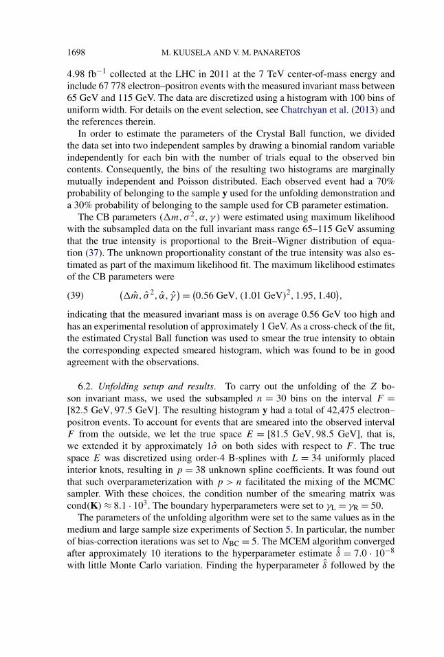
4.98 fb−1 collected at the LHC in 2011 at the 7 TeV center-of-mass energy andinclude 67 778 electron–positron events with the measured invariant mass between65 GeV and 115 GeV. The data are discretized using a histogram with 100 bins ofuniform width. For details on the event selection, see Chatrchyan et al. (2013) andthe references therein.

In order to estimate the parameters of the Crystal Ball function, we dividedthe data set into two independent samples by drawing a binomial random variableindependently for each bin with the number of trials equal to the observed bincontents. Consequently, the bins of the resulting two histograms are marginallymutually independent and Poisson distributed. Each observed event had a 70%probability of belonging to the sample y used for the unfolding demonstration anda 30% probability of belonging to the sample used for CB parameter estimation.

The CB parameters (�m,σ 2, α, γ ) were estimated using maximum likelihoodwith the subsampled data on the full invariant mass range 65–115 GeV assumingthat the true intensity is proportional to the Breit–Wigner distribution of equa-tion (37). The unknown proportionality constant of the true intensity was also es-timated as part of the maximum likelihood fit. The maximum likelihood estimatesof the CB parameters were(

�m, σ 2, α, γ) = (

0.56 GeV, (1.01 GeV)2,1.95,1.40),(39)

indicating that the measured invariant mass is on average 0.56 GeV too high andhas an experimental resolution of approximately 1 GeV. As a cross-check of the fit,the estimated Crystal Ball function was used to smear the true intensity to obtainthe corresponding expected smeared histogram, which was found to be in goodagreement with the observations.

6.2. Unfolding setup and results. To carry out the unfolding of the Z bo-son invariant mass, we used the subsampled n = 30 bins on the interval F =[82.5 GeV,97.5 GeV]. The resulting histogram y had a total of 42,475 electron–positron events. To account for events that are smeared into the observed intervalF from the outside, we let the true space E = [81.5 GeV,98.5 GeV], that is,we extended it by approximately 1σ on both sides with respect to F . The truespace E was discretized using order-4 B-splines with L = 34 uniformly placedinterior knots, resulting in p = 38 unknown spline coefficients. It was found outthat such overparameterization with p > n facilitated the mixing of the MCMCsampler. With these choices, the condition number of the smearing matrix wascond(K) ≈ 8.1 · 103. The boundary hyperparameters were set to γL = γR = 50.

The parameters of the unfolding algorithm were set to the same values as in themedium and large sample size experiments of Section 5. In particular, the numberof bias-correction iterations was set to NBC = 5. The MCEM algorithm convergedafter approximately 10 iterations to the hyperparameter estimate δ = 7.0 · 10−8

with little Monte Carlo variation. Finding the hyperparameter δ followed by the


FIG. 4. Unfolding of the Z boson invariant mass spectrum. The confidence band consists of the95% pointwise percentile intervals of the bias-corrected estimator obtained using 5 bias-correctioniterations. The points show a histogram estimate of the smeared intensity.

point estimate f took 10 minutes, while the running time to obtain the bias-corrected confidence intervals was approximately 17 hours.

In Figure 4, the unfolded intensity f and the 95% pointwise percentile intervalsof the bias-corrected intensity fBC are compared with the Breit–Wigner shape ofthe Z boson mass peak. The proportionality constant of the true intensity was ob-tained from the maximum likelihood fit described in Section 6.1. The figure alsoshows a histogram estimate of the smeared intensity given by the observed eventcounts y divided by the 0.5 GeV bin width. The unfolding algorithm is able tocorrectly reconstruct the location and width of the Z mass peak which are bothdistorted by the smearing in the ECAL. The intensity is also estimated reasonablywell in the 1 GeV regions in the tails of the intensity where no smeared observa-tions were available. More importantly, the 95% bias-corrected confidence inter-vals cover the true mass peak across the whole invariant mass spectrum. We alsoobserve that the bias-correction is particularly important near the top of the masspeak, where the original point estimate f appears to be somewhat biased.

7. Concluding remarks. We have studied a novel approach to solving thehigh energy physics unfolding problem involving empirical Bayes selection of theregularization strength and frequentist uncertainty quantification using an iterativebias-correction. We have shown that empirical Bayes provides a straightforward,fully data-driven way of choosing the hyperparameter δ and demonstrated that themethod provides good estimates of the regularization strength with both simulated


and real data. Given the good performance of the approach, we anticipate empiricalBayes methods to also be valuable in solving other inverse problems beyond theunfolding problem.

The natural fully Bayesian alternative to empirical Bayes consists of using aBayesian hierarchical model which necessitates the choice of a hyperprior for δ.Unfortunately, the resulting estimates are known to be sensitive to this nontriv-ial choice [Gelman (2006)]. We provide in the online supplement [Kuusela andPanaretos (2015)] a comparison of empirical Bayes and hierarchical Bayes for anumber of uninformative hyperpriors. Our results indicate that the relative pointestimation performance of the methods depends strongly on the choice of the hy-perprior, especially when there is only a limited amount of data. For example, inthe small sample size experiment of Section 5, the integrated squared error of hier-archical Bayes ranges from 17% better to 30% worse than that of empirical Bayesdepending on the choice of the hyperprior. Unfortunately, there are no guaranteesthat the uninformative hyperprior that worked the best in this example would al-ways provide the best performance. These results also indicate that hyperpriorswhich were designed to be uninformative are actually fairly informative in hier-archical Bayes unfolding and have an undesirably large influence on the unfoldedresults, while empirical Bayes achieves comparable point estimation performancewithout the need to make any arbitrary distributional assumptions on δ. The hi-erarchical Bayes credible intervals also suffer from similar coverage issues as theempirical Bayes credible intervals.

The other main component of our approach is frequentist uncertainty quantifi-cation using an iterative bias-correction technique. We have shown that the bias-correction is crucial for establishing close-to-nominal frequentist coverage andthat, at least within the context of our simulation study, the approach outperformsexisting techniques based on bootstrap resampling and Bayesian credible intervals.The good performance of this approach raises many interesting questions for fu-ture work. For example, there seems to be a trade-off between the coverage and thelength of the bias-corrected intervals and this trade-off is governed by the numberof bias-correction iterations NBC. That is, it appears that one is able to obtain con-sistently better coverage by running more bias-correction iterations at the expenseof increased interval length. By studying the theoretical properties of the iteration,one might be able to provide guidance on how to choose NBC in such a way thatit optimizes the length of the intervals while maintaining the coverage within apreset threshold of the nominal value.

In this work, we have focused on the most basic inferential tool in nonparamet-ric statistics, that is, we have aimed at building pointwise confidence bands forthe unknown intensity f with good frequentist coverage properties. These bandscan be directly used for making pointwise inferential statements, such as testingif the data are consistent with some theoretical prediction of f at a single points ∈ E chosen before seeing the data. They also form the basis for making morecomplicated inferences. For example, one can envisage using the bands for testing


whether the data are consistent with a theoretical prediction at several locations orover the whole spectrum by making a multiple testing correction. The appropri-ate form of the inferential statement depends, however, on the original purpose ofthe unfolding operation and each purpose listed in Section 2.2 involves differenttypes of inferential goals, including the comparison and combination of severalunfolded measurements. Extensions of the tools studied in this paper to such morecomplicated situations constitutes an important topic for future work.

It should also be noted that throughout this paper the confidence intervals arecomputed for a fixed forward mapping K , while in reality there is usually a system-atic uncertainty associated with K stemming from the fact that K is typically esti-mated using either simulations or some auxiliary measurements. In cases where thedetector response can be modeled using a parametric model, such as the Z bosonexample of Section 6, the unknown parameters can be estimated using maximumlikelihood on data generated by a known true intensity. More generally, however,one may need to consider nonparametric estimates of K . Once an estimate of K

has been obtained, it is likely that its uncertainty can be incorporated into the outerbootstrap loop of the bias-corrected confidence intervals. A detailed study of theseideas will be the subject of future work by the authors.

Finally, it should be pointed out that it is possible to find situations where theproposed unfolding methodology will not yield good reconstructions. This hap-pens when the smoothness penalty, that is, penalizing for large values of ‖f ′′‖2

2,is not the appropriate way of regularizing the problem. For instance, if the trueintensity f contains sharp peaks or rapid oscillations, the solution would poten-tially be biased to an extent where the iterative bias-correction would be unableto adequately improve the situation. In particular, the penalty would be unlikelyto adapt well to situations where the magnitude of the second derivative variessignificantly across the spectrum. This is the case, for example, when the inten-sity contains features at very different spatial scales or when it corresponds to asteeply falling spectrum that varies over many orders of magnitude. Naturally, inthese cases, a more suitable choice of the family of regularizing priors {p(β|δ)}δ>0should fix the problem. For example, in the case of a steeply falling spectrum, onecould consider penalizing for the second derivative of logf instead of f or usinga spatially adaptive smoothness penalty [Pintore, Speckman and Holmes (2006)].These considerations highlight the fact that all the inferences considered here arecontingent on the chosen family of regularizing priors and should be interpretedwith this in mind.

Acknowledgments. We wish to warmly thank Bob Cousins, Anthony Davi-son, Tommaso Dorigo, Louis Lyons and Mikko Voutilainen for insightful discus-sions and their encouragement in the course of this work. We are also gratefulto the Associate Editor and the two anonymous reviewers for their exceptionallydetailed and constructive feedback.


SUPPLEMENTARY MATERIAL

Supplement to “Statistical unfolding of elementary particle spectra: Em-pirical Bayes estimation and bias-corrected uncertainty quantification” (DOI:10.1214/15-AOAS857SUPP; .pdf). The supplement provides a comparison of theempirical Bayes and hierarchical Bayes approaches to unfolding; additional sim-ulations results complementing those of Section 5; and technical material on theconvergence and mixing of the MCMC sampler and on the Gaussian approxima-tion used in the coverage studies.

REFERENCES

AAD, G. et al. (2012). Measurement of the transverse momentum distribution of W bosons in pp

collisions at√

s = 7 TeV with the ATLAS detector. Phys. Rev. D 85 012005.ANTONIADIS, A. and BIGOT, J. (2006). Poisson inverse problems. Ann. Statist. 34 2132–2158.

MR2291495BARDSLEY, J. M. and GOLDES, J. (2009). Regularization parameter selection methods for ill-posed

Poisson maximum likelihood estimation. Inverse Probl. 25 095005. MR2540885BARNEY, D. (2004). CMS-doc-4172. Available at https://cms-docdb.cern.ch/cgi-bin/PublicDocDB/

ShowDocument?docid=4172. Retrieved 21.1.2014.BERINGER, J. et al. (2012). Review of particle physics. Phys. Rev. D 86 010001.BISHOP, C. M. (2006). Pattern Recognition and Machine Learning. Springer, New York.

MR2247587BLOBEL, V. (1985). Unfolding methods in high-energy physics experiments. In Proceedings of the

1984 CERN School of Computing (C. Verkern, ed.) CERN 85-09 88-127. CERN, Geneva.BLOBEL, V. (2013). Unfolding. In Data Analysis in High Energy Physics: A Practical Guide to

Statistical Methods (O. Behnke, K. Kröninger, G. Schott and T. Schörner-Sadenius, eds.) 187–225. Wiley-VCH, Weinheim.

BOCHKINA, N. (2013). Consistency of the posterior distribution in generalized linear inverse prob-lems. Inverse Probl. 29 095010, 43. MR3094485

BOOTH, J. G. and HOBERT, J. P. (1999). Maximizing generalized linear mixed model likelihoodswith an automated Monte Carlo EM algorithm. J. R. Stat. Soc. Ser. B. Stat. Methodol. 61 265–285.

CALVETTI, D., KAIPIO, J. P. and SOMERALO, E. (2006). Aristotelian prior boundary conditions.Int. J. Math. Comput. Sci. 1 63–81. MR2232301

CARLIN, B. P. and LOUIS, T. A. (2009). Bayesian Methods for Data Analysis, 3rd ed. CRC Press,Boca Raton, FL. MR2442364

CASELLA, G. (2001). Empirical Bayes Gibbs sampling. Biostatistics 2 485–500.CHATRCHYAN, S. et al. (2008). The CMS experiment at the CERN LHC. Journal of Instrumentation

3 S08004.CHATRCHYAN, S. et al. (2009). Particle-flow event reconstruction in CMS and performance for jets,

taus, and EmissT . CMS Physics Analysis Summary CMS-PAS-PFT-09-001.

CHATRCHYAN, S. et al. (2012a). Shape, transverse size, and charged-hadron multiplicity of jets inpp collisions at

√s = 7 TeV. J. High Energy Phys. 06 160.

CHATRCHYAN, S. et al. (2012b). Measurement of the charge asymmetry in top-quark pair productionin proton–proton collisions at

√s = 7 TeV. Phys. Lett. B 709 28–49.

CHATRCHYAN, S. et al. (2012c). Observation of a new boson at a mass of 125 GeV with the CMSexperiment at the LHC. Phys. Lett. B 716 30–61.

CHATRCHYAN, S. et al. (2013). Energy calibration and resolution of the CMS electromagneticcalorimeter in pp collisions at

√s = 7 TeV. Journal of Instrumentation 8 P09009.

http://dx.doi.org/10.1214/15-AOAS857SUPP

http://www.ams.org/mathscinet-getitem?mr=2291495


https://cms-docdb.cern.ch/cgi-bin/PublicDocDB/ShowDocument?docid=4172





https://cms-docdb.cern.ch/cgi-bin/PublicDocDB/ShowDocument?docid=4172


CHOUDALAKIS, G. (2012). Fully Bayesian unfolding. Available at arXiv:1201.4612v4[physics.data-an].

COWAN, G. (1998). Statistical Data Analysis. Oxford Univ. Press, London.D’AGOSTINI, G. (1995). A multidimensional unfolding method based on Bayes’ theorem. Nuclear

Instruments and Methods in Physics Research A 362 487–498.DAVISON, A. C. and HINKLEY, D. V. (1997). Bootstrap Methods and Their Application. Cam-

bridge Series in Statistical and Probabilistic Mathematics 1. Cambridge Univ. Press, Cambridge.MR1478673

DE BOOR, C. (2001). A Practical Guide to Splines, revised ed. Applied Mathematical Sciences 27.Springer, New York. MR1900298

DE BOOR, C. and DANIEL, J. W. (1974). Splines with nonnegative B-spline coefficients. Math.Comp. 28 565–568. MR0378357

DEMBINSKI, H. P. and ROTH, M. (2011). ARU—Towards automatic unfolding of detector effects.In Proceedings of the PHYSTAT 2011 Workshop on Statistical Issues Related to Discovery Claimsin Search Experiments and Unfolding (H. B. Prosper and L. Lyons, eds.) CERN-2011-006 285–291. CERN, Geneva.

DEMPSTER, A. P., LAIRD, N. M. and RUBIN, D. B. (1977). Maximum likelihood from incompletedata via the EM algorithm. J. R. Stat. Soc. Ser. B. Stat. Methodol. 39 1–38. MR0501537

EFRON, B. and TIBSHIRANI, R. J. (1993). An Introduction to the Bootstrap. Monographs on Statis-tics and Applied Probability 57. Chapman & Hall, New York. MR1270903

EILERS, P. H. C. and MARX, B. D. (1996). Flexible smoothing with B-splines and penalties. Statist.Sci. 11 89–121. MR1435485

ENGL, H. W., HANKE, M. and NEUBAUER, A. (2000). Regularization of Inverse Problems. KluwerAcademic Publishers, Dordrecht.

GELMAN, A. (2006). Prior distributions for variance parameters in hierarchical models (commenton article by Browne and Draper). Bayesian Anal. 1 515–533. MR2221284

GEMAN, S. and MCCLURE, D. E. (1985). Bayesian image analysis: An application to single photonemission tomography. In Proceedings of the Statistical Computing Section 12–18. Amer. Statist.Assoc., Alexandria, VA.

GEMAN, S. and MCCLURE, D. E. (1987). Statistical methods for tomographic image reconstruction.Bull. Inst. Internat. Statist. 52 5–21. MR1027188

GILKS, W. R. (1996). Full conditional distributions. In Markov Chain Monte Carlo in Practice(W. R. Gilks, S. Richardson and D. J. Spiegelhalter, eds.) 75–88. Chapman & Hall, London.MR1397966

GILKS, W. R., RICHARDSON, S. and SPIEGELHALTER, D. J. (1996). Markov Chain Monte Carloin Practice. Chapman & Hall, London. MR1397966

GOLDSTEIN, H. (1996). Consistent estimators for multilevel generalized linear models using aniterated bootstrap. Multilevel Modelling Newsletter 8 3–6.

HÖCKER, A. and KARTVELISHVILI, V. (1996). SVD approach to data unfolding. Nuclear Instru-ments and Methods in Physics Research A 372 469–481.

JAVANMARD, A. and MONTANARI, A. (2014). Confidence intervals and hypothesis testing for high-dimensional regression. J. Mach. Learn. Res. 15 2869–2909. MR3277152

KAIPIO, J. and SOMERSALO, E. (2005). Statistical and Computational Inverse Problems. AppliedMathematical Sciences 160. Springer, New York. MR2102218

KUK, A. Y. C. (1995). Asymptotically unbiased estimation in generalized linear models with ran-dom effects. J. R. Stat. Soc. Ser. B. Stat. Methodol. 57 395–407. MR1323346

KUUSELA, M. and PANARETOS, V. M. (2015). Supplement to “Statistical unfolding of elemen-tary particle spectra: Empirical Bayes estimation and bias-corrected uncertainty quantification.”DOI:10.1214/15-AOAS857SUPP.

LUCY, L. B. (1974). An iterative technique for the rectification of observed distributions. Astronom-ical Journal 79 745–754.

http://arxiv.org/abs/arXiv:1201.4612v4














http://dx.doi.org/10.1214/15-AOAS857SUPP


LYONS, L. (2011). Unfolding: Introduction. In Proceedings of the PHYSTAT 2011 Workshop on Sta-tistical Issues Related to Discovery Claims in Search Experiments and Unfolding (H. B. Prosperand L. Lyons, eds.) CERN-2011-006 225–228. CERN, Geneva.

LYONS, L. (2013). Bayes and frequentism: A particle physicist’s perspective. Contemporary Physics54 1–16.

MCLACHLAN, G. J. and KRISHNAN, T. (2008). The EM Algorithm and Extensions, 2nd ed. Wiley,Hoboken, NJ. MR2392878

MEISTER, A. (2009). Deconvolution Problems in Nonparametric Statistics. Lecture Notes in Statis-tics 193. Springer, Berlin. MR2768576

MILKE, N., DOERT, M., KLEPSER, S., MAZIN, D., BLOBEL, V. and RHODE, W. (2013). Solvinginverse problems with the unfolding program TRUEE: Examples in astroparticle physics. NuclearInstruments and Methods in Physics Research A 697 133–147.

MOROZOV, V. A. (1966). On the solution of functional equations by the method of regularization.Soviet Math. Dokl. 7 414–417. MR0208819

NYCHKA, D. (1988). Bayesian confidence intervals for smoothing splines. J. Amer. Statist. Assoc.83 1134–1143. MR0997592

O’SULLIVAN, F. (1986). A statistical perspective on ill-posed inverse problems. Statist. Sci. 1 502–527. MR0874480

O’SULLIVAN, F. (1988). Fast computation of fully automated log-density and log-hazard estimators.SIAM J. Sci. Statist. Comput. 9 363–379. MR0930052

OREGLIA, M. J. (1980). A study of the reactions ψ ′ → γ γψ . Ph.D. thesis, Stanford Univ.PANARETOS, V. M. (2011). A statistician’s view on deconvolution and unfolding. In Proceedings

of the PHYSTAT 2011 Workshop on Statistical Issues Related to Discovery Claims in SearchExperiments and Unfolding (H. B. Prosper and L.Lyons, eds.) CERN-2011-006 229–239. CERN,Geneva.

PINTORE, A., SPECKMAN, P. and HOLMES, C. C. (2006). Spatially adaptive smoothing splines.Biometrika 93 113–125. MR2277744

PROSPER, H. B. and LYONS, L., eds. (2011). Proceedings of the PHYSTAT 2011 Workshop onStatistical Issues Related to Discovery Claims in Search Experiments and Unfolding. CERN-2011-006. CERN, Geneva.

RASMUSSEN, C. E. and WILLIAMS, C. K. I. (2006). Gaussian Processes for Machine Learning.MIT Press, Cambridge, MA. MR2514435

REISS, R.-D. (1993). A Course on Point Processes. Springer, New York. MR1199815RICHARDSON, W. H. (1972). Bayesian-based iterative method of image restoration. J. Opt. Soc.

Amer. A 62 55–59.ROBERT, C. P. and CASELLA, G. (2004). Monte Carlo Statistical Methods, 2nd ed. Springer, New

York. MR2080278RUPPERT, D. and CARROLL, R. J. (2000). Spatially-adaptive penalties for spline fitting. Aust. N.Z.

J. Stat. 42 205–223.RUPPERT, D., WAND, M. P. and CARROLL, R. J. (2003). Semiparametric Regression. Cambridge

Series in Statistical and Probabilistic Mathematics 12. Cambridge Univ. Press, Cambridge.MR1998720

SAQUIB, S. S., BOUMAN, C. A. and SAUER, K. (1998). ML parameter estimation for Markovrandom fields with applications to Bayesian tomography. IEEE Trans. Image Process. 7 1029–1044.

SCHUMAKER, L. L. (2007). Spline Functions: Basic Theory, 3rd ed. Cambridge Univ. Press, Cam-bridge. MR2348176

STONE, M. (1974). Cross-validatory choice and assessment of statistical predictions. J. R. Stat. Soc.Ser. B. Stat. Methodol. 36 111–147. MR0356377

VARDI, Y., SHEPP, L. A. and KAUFMAN, L. (1985). A statistical model for positron emissiontomography. J. Amer. Statist. Assoc. 80 8–37. MR0786595
















VEKLEROV, E. and LLACER, J. (1987). Stopping rule for the MLE algorithm based on statisticalhypothesis testing. IEEE Trans. Med. Imaging 6 313–319.

WAHBA, G. (1983). Bayesian “confidence intervals” for the cross-validated smoothing spline. J. R.Stat. Soc. Ser. B. Stat. Methodol. 45 133–150. MR0701084

WAHBA, G. (1990). Spline Models for Observational Data. CBMS-NSF Regional Conference Seriesin Applied Mathematics 59. SIAM, Philadelphia, PA. MR1045442

WEI, G. C. G. and TANNER, M. A. (1990). A Monte Carlo implementation of the EM algorithmand the poor man’s data augmentation algorithms. J. Amer. Statist. Assoc. 85 699–704.

WEIR, I. S. (1997). Fully Bayesian reconstructions from single-photon emission computed tomog-raphy data. J. Amer. Statist. Assoc. 92 49–60.

WOOD, S. N. (2006). On confidence intervals for generalized additive models based on penalizedregression splines. Aust. N.Z. J. Stat. 48 445–464. MR2329279

WOOD, S. N. (2011). Fast stable restricted maximum likelihood and marginal likelihood estimationof semiparametric generalized linear models. J. R. Stat. Soc. Ser. B. Stat. Methodol. 73 3–36.MR2797734

SECTION DE MATHÉMATIQUES

ÉCOLE POLYTECHNIQUE FÉDÉRALE DE LAUSANNE

EPFL STATION 8, 1015 LAUSANNE

SWITZERLAND

E-MAIL: [email protected]@epfl.ch





mailto:[email protected]

mailto:[email protected]

Documents

Statistical unfolding of elementary particle spectra: …smat.epfl.ch/victor/papers/KuuselaPanaretos_AOAS2015.pdf · 2015-11-03 · STATISTICAL UNFOLDING OF ELEMENTARY PARTICLE SPECTRA: