Statistical treatment of grain-size curves and empirical distributions:densities as compositions?

R. Tolosana-Delgado1, K.G. van den Boogaart2, T. Mikes1 and H. von Eynatten1

1Georg-August University, Gottingen, Germany; raimon.tolosana@geo.uni-goettingen.de2Ernst-Moritz-Arndt University, Greifswald, Germany.

Abstract

The preceding two editions of CoDaWork included talks on the possible considerationof densities as infinite compositions: Egozcue and Dıaz-Barrero (2003) extended theEuclidean structure of the simplex to a Hilbert space structure of the set of densitieswithin a bounded interval, and van den Boogaart (2005) generalized this to the setof densities bounded by an arbitrary reference density. From the many variations ofthe Hilbert structures available, we work with three cases. For bounded variables, abasis derived from Legendre polynomials is used. For variables with a lower bound, westandardize them with respect to an exponential distribution and express their densitiesas coordinates in a basis derived from Laguerre polynomials. Finally, for unboundedvariables, a normal distribution is used as reference, and coordinates are obtained withrespect to a Hermite-polynomials-based basis.

To get the coordinates, several approaches can be considered. A numerical accuracyproblem occurs if one estimates the coordinates directly by using discretized scalarproducts. Thus we propose to use a weighted linear regression approach, where all k-order polynomials are used as predictand variables and weights are proportional to thereference density. Finally, for the case of 2-order Hermite polinomials (normal reference)and 1-order Laguerre polinomials (exponential), one can also derive the coordinatesfrom their relationships to the classical mean and variance.

Apart of these theoretical issues, this contribution focuses on the application of thistheory to two main problems in sedimentary geology: the comparison of several grainsize distributions, and the comparison among different rocks of the empirical distri-bution of a property measured on a batch of individual grains from the same rock orsediment, like their composition.

Key words: probability measure, granulometry, size composition, non-parametricrepresentation of probability density

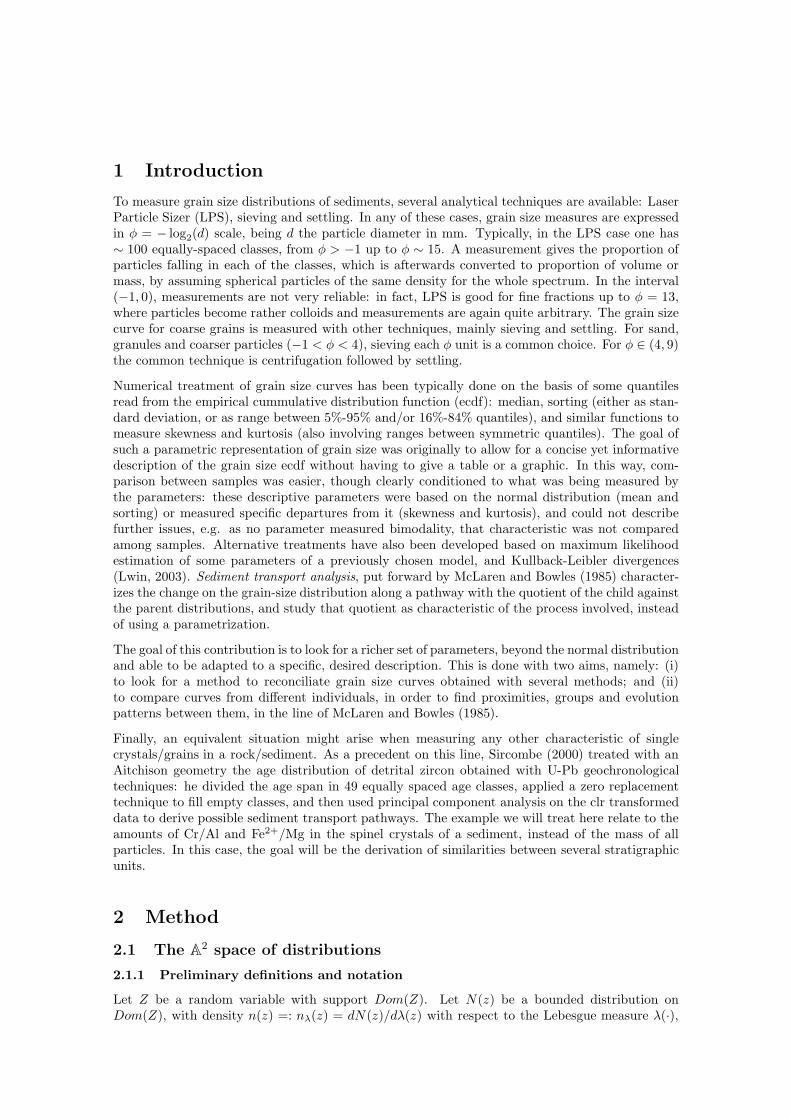
1 Introduction

To measure grain size distributions of sediments, several analytical techniques are available: LaserParticle Sizer (LPS), sieving and settling. In any of these cases, grain size measures are expressedin φ = − log2(d) scale, being d the particle diameter in mm. Typically, in the LPS case one has∼ 100 equally-spaced classes, from φ > −1 up to φ ∼ 15. A measurement gives the proportion ofparticles falling in each of the classes, which is afterwards converted to proportion of volume ormass, by assuming spherical particles of the same density for the whole spectrum. In the interval(−1, 0), measurements are not very reliable: in fact, LPS is good for fine fractions up to φ = 13,where particles become rather colloids and measurements are again quite arbitrary. The grain sizecurve for coarse grains is measured with other techniques, mainly sieving and settling. For sand,granules and coarser particles (−1 < φ < 4), sieving each φ unit is a common choice. For φ ∈ (4, 9)the common technique is centrifugation followed by settling.

Numerical treatment of grain size curves has been typically done on the basis of some quantilesread from the empirical cummulative distribution function (ecdf): median, sorting (either as stan-dard deviation, or as range between 5%-95% and/or 16%-84% quantiles), and similar functions tomeasure skewness and kurtosis (also involving ranges between symmetric quantiles). The goal ofsuch a parametric representation of grain size was originally to allow for a concise yet informativedescription of the grain size ecdf without having to give a table or a graphic. In this way, com-parison between samples was easier, though clearly conditioned to what was being measured bythe parameters: these descriptive parameters were based on the normal distribution (mean andsorting) or measured specific departures from it (skewness and kurtosis), and could not describefurther issues, e.g. as no parameter measured bimodality, that characteristic was not comparedamong samples. Alternative treatments have also been developed based on maximum likelihoodestimation of some parameters of a previously chosen model, and Kullback-Leibler divergences(Lwin, 2003). Sediment transport analysis, put forward by McLaren and Bowles (1985) character-izes the change on the grain-size distribution along a pathway with the quotient of the child againstthe parent distributions, and study that quotient as characteristic of the process involved, insteadof using a parametrization.

The goal of this contribution is to look for a richer set of parameters, beyond the normal distributionand able to be adapted to a specific, desired description. This is done with two aims, namely: (i)to look for a method to reconciliate grain size curves obtained with several methods; and (ii)to compare curves from different individuals, in order to find proximities, groups and evolutionpatterns between them, in the line of McLaren and Bowles (1985).

Finally, an equivalent situation might arise when measuring any other characteristic of singlecrystals/grains in a rock/sediment. As a precedent on this line, Sircombe (2000) treated with anAitchison geometry the age distribution of detrital zircon obtained with U-Pb geochronologicaltechniques: he divided the age span in 49 equally spaced age classes, applied a zero replacementtechnique to fill empty classes, and then used principal component analysis on the clr transformeddata to derive possible sediment transport pathways. The example we will treat here relate to theamounts of Cr/Al and Fe2+/Mg in the spinel crystals of a sediment, instead of the mass of allparticles. In this case, the goal will be the derivation of similarities between several stratigraphicunits.

2 Method

2.1 The A2 space of distributions

2.1.1 Preliminary definitions and notation

Let Z be a random variable with support Dom(Z). Let N(z) be a bounded distribution onDom(Z), with density n(z) =: nλ(z) = dN(z)/dλ(z) with respect to the Lebesgue measure λ(·),

i.e.

0 <

∫

Dom(Z)

n(z)dλ(z) =

∫

Dom(Z)

dN(z) < +∞,

and giving some probability to each subset of Dom(Z), thus n(z) > 0, ∀z ∈ Dom(Z). Thisdistribution is considered the reference distribution, and will play the role of origin of the followingspace. Take A

2(n) as the set of possible distributions F (z) on Dom(Z) with square-integrablelog-density with respect to N(z),

∫

Dom(Z)

log2

(dF (z)

dN(z)

)

dN(z) = EN

[

log2

(dF (z)

dN(z)

)]

< ∞,

where

fN (z) =dF (z)

dN(z)=

dF (z)/dλ(z)

dN(z)/dλ(z)=

fλ(z)

nλ(z)

is the density of F (z) with respect to N(z). From now on, we will consider N(z)—or n(z), beingunivocally linked—fixed and known, and we will not specify any more that densities are computedwith respect to it.

Let f and g be two elements of A2(n), and µ ∈ R a real value. We will say that f and g are

equivalent in an Aitchison sense, written f =A g, if there exists a unique positive scalar µ fulfilling

f(z) = µ · g(z), ∀z ∈ Dom(Z). (1)

This defines an equivalence class. For those equivalence classes with bounded integral, one cantake the representative of the class as the one being a true probability density (i.e., integral one).

2.1.2 Hilbert space structure

The following two operations

f ⊕ g =A f(z) · g(z) and µ ⊙ f =A fµ(z), (2)

called perturbation and power transformation, define a vector space structure on A2(n). The

operation

clr(f) = log f(z) −∫

Dom(Z)

log f(z)dN(z) (3)

allows the definition of a scalar product on A2(n), namely

〈f, g〉 =

∫

Dom(Z)

clr(f)clr(g)dN(z), (4)

building a full Hilbert space structure on A2(n), according to van den Boogaart (2005).

To interpret these operations, the power operation perfectly describes arbitrary sediment sorting, asit keeps the position of the modes but increases its “peakness”, or reduces its dispersion. Regardingperturbation, note that in McLaren and Bowles (1985) approach, the difference between two grain-size distributions would be measured as g(z)/f(z), which is equivalent to (2) without reclosure.Following these authors, if g(z) is the distribution of a daughter sediment of a parent sedimentwith grain size curve f(z), then

• nett erosion of new sediment would be characterized by a curve g ⊖ f with marked negativeskewness,

• nett accretion produce a curve g ⊖ f with marked positive skewness,

• a dinamic equilibrium between these two generates symmetric g ⊖ f curves,

• sediment deposition forms“heavy tailed”g⊖f curves on those grain sizes which are not beingdeposited,

2.1.3 Exponential families

A K-parametric exponential family is a set of densities such that any of them can be expressed asthe product of three positive functions

f(z|ϕ1, ϕ2, . . . , ϕK) = A(ϕ1, ϕ2, . . . , ϕK) · exp

[K∑

k=1

ϕk · Tk(z)

]

· g(z),

this is, a function A(·) of the parameters only, a function g(z) only of the random variable, andthe exponential of a linear interaction function. Taking g(z) = n(z), one finds that exponentialfamilies can be understood as K-dimensional subspaces of A

2(n), being the vectors of the basisek(z) =A exp (Tk(z)). Then, A(·) can be ignored without risk, as it just closes the density tointegral one, i.e. chooses the probability representative of the equivalence class (van den Boogaart,2005).

2.1.4 Coordinates

Let πk(z) be a series of functions with natural index k, such that π0(z) ∝ 1 and they are orthonor-mal with respect to the density n(z), i.e.

∫

Dom(Z)

πi(z) · πj(z) · n(z)dz = δij . (5)

These functions allow to define an orthonormal basis of A2(n), by taking

pk(z) =A exp[πk(z)] k > 0.

The k-th coordinate ϕk with respect to this basis may be computed with (van den Boogaart, 2005).

ϕk = 〈f, pk〉 =

∫

Dom(Z)

clr(f(z))πk(z)dN(z). (6)

2.2 Three particular cases

2.2.1 The classical densities

Three particular cases will be of interest for our practical applications, all three using ortogonalpolynomials satisfying Eq. (5) to induce the basis, and all three generalizing a density from anexponential family. These are described in Table 1, containing:

• the name of the family

• the reference density

• the support of the underlying random variable

• the name of the orthogonal polynomials inducing the basis

• the orthonormal polynomials defining the basis of the subspace in which the conventionalfamily is defined

• the coordinates of the conventional family in this basis

• the dimension of the subspace,

• and the boundary between proper densities and those with infinite integral.

Table 1: characteristics of the three reference models, and their relation to known probability densities.

name normal exponential uniform

n(z) 1√2π

exp(− z2

2 ) exp(−z) 12I(z ∈ Dom(Z))

Dom(Z) (−∞, +∞) (0, +∞) (−1, +1)polynomials Hermite Laguerre Legendre

π1(z) z z —

π2(z) 1−z2

√2

— —

ϕ1µσ2 λ − 1 —

ϕ21−σ2

√2σ2

— —

dimension 2 1 0boundary ϕ2 > − 1√

2ϕ1 > −1 —

For instance, when working with a standard normal distribution as reference and using Hermitepolynomials to define the basis, if we restrict our densities to a two-dimensional subspace of A

2(n)(K = 2), then the resulting subspace contains all possible normal densities, as for instance

fN (z|µ, σ) =

1√2πσ

exp[

− (z−µ)2

2σ2

]

1√2π

exp[− z2

2

] =1

σexp

[

− (z − µ)2

2σ2+

z2

2

]

=

=A exp

[

−z2 + µ2 − 2µz − σ2z2

2σ2

]

=A exp

[

−z2 − 2µz − σ2z2

2σ2

]

=

=A exp

[1 − σ2

2σ2− 1 − σ2

2σ2− (1 − σ2)z2 − 2µz

2σ2

]

=

=A exp

[1 − σ2

2σ2− (1 − σ2)z2 − 2µz

2σ2

]

=

= exp

[

− (1 − σ2)(1 − z2) + 2µz

2σ2

]

= exp

[1 − σ2

√2σ2

1 − z2

√2

+µ

σ2z

]

=

=A

µ

σ2⊙ eπ1(z) ⊕ 1 − σ2

√2σ2

⊙ eπ2(z) = ϕ1 ⊙ eπ1(z) ⊕ ϕ2 ⊙ eπ2(z).

(The notation =A is used when the two members of the equality are equivalent in Aitchison sense,that is: from one to the other an element was added or removed, which is a multiplicative functionof the paramerers only, not of the variable z). Note that, in this case we know that the result willonly be a probability density (i.e., with finite integral) iff σ2 > 0, which implies that ϕ2 > −1/

√2.

On the contrary, ϕ1 = µ/σ2 can take any value. Thus, the set of densities is a 2-dimensionalhalf-subspace of A

2(n), with the other half containing measures with infinite integral.

2.2.2 Densities of higher dimension

If we allow more polynomials in the basis, resulting densities will no longer be of the normalfamily, and even these relationships between means, variance and coordinates will not be satisfiedany more. In this case, results will only be probability densities if the maximum degree of thepolynomials (K, dimension of the subspace) is even, and its coordinate ϕK is negative: theseconditions ensure that the log-density decreases towards both ±∞. Similar conditions must beimposed in the exponential family to ensure proper densities: as the density is defined for z > 0,one has to ensure that the resulting polynomials will decrease towards +∞, that is its highest degreeterm must have a negative coefficient, be it even or odd. Table 2 summarizes these conditions.

Interestingly, the range of shapes that can be displayed by the resulting densities is much broaderthan those of their parent classical distributions (Fig. 1),

Table 2: boundaries on the parameter space between proper and improper densities, for the three reference models.

name normal exponential uniformmaximum K even any any

ϕK < 0 < 0 no condition

• the maximum number of (derivable) modes is equal to K/2 (or the biggest integer below it),though with the exponential one can have another maximum extreme at z = 0, and with theuniform the same can happen in any one or both extremes (z = ±1),

• in the normal and uniform case, the skewness is fundamentally controlled by the odd co-ordinates, as even polynomials contain only even degrees and have thus always symmetriccontributions,

• polymodality in the normal and uniform cases is controlled by the difference between thecoefficients of the highest degree and the following even coefficient.

−3 −2 −1 0 1 2 3

0.0

0.1

0.2

0.3

0.4

0.5

0.6

z

dens

ity

Figure 1: Several examples of densities of the exponential family formed by the normal density (bold black line)and the first 4 Hermite polynomials, with the following coordinates:

colour ϕ1 ϕ2 ϕ3 ϕ4

red 0.00 -0.50 0.00 -0.50

green3 0.00 -0.50 0.50 -0.50

blue 0.00 -0.50 1.00 -0.50

cyan 0.00 -0.50 0.00 -1.50

magenta 0.00 -0.50 -1.00 -1.50

2.3 Discrete approximations to coordinate computation

With empirical data, one will almost always have just a discretized version of the densities ordistributions, not the functions themselves. These can be for instance,

• a kernel-density estimation of the distribution of a sample

• the laser particle sizer measurement of the granulometric curve of a sediment

• a kernel-density approximation of the sieving measurement of the granulometric curve of asediment

Equation (6) will thus be very rarely useful to obtain the coordinates of these functions. A firstidea is to try a quadrature approximation. Let z1, . . . , zM be a set of M equally spaced pointsin Dom(Z), and f1, . . . , fM and n1, . . . , nM the values of the target density fm ∝ f(zm) and thereference density nm ∝ n(zm) on these points, the last one forced to sum up to one. Then weshould have

ϕk ≈M∑

m=1

clr(fm) · πk(zm) · nm,

with

clr(fm) = logfm

nm

−M∑

i=1

ni logfi

ni

(7)

But we should also verify that the orthonormality conditions hold (Eq. 5), i.e.

M∑

m=1

πj(zm) · πk(zm) · nm ≈ δjk.

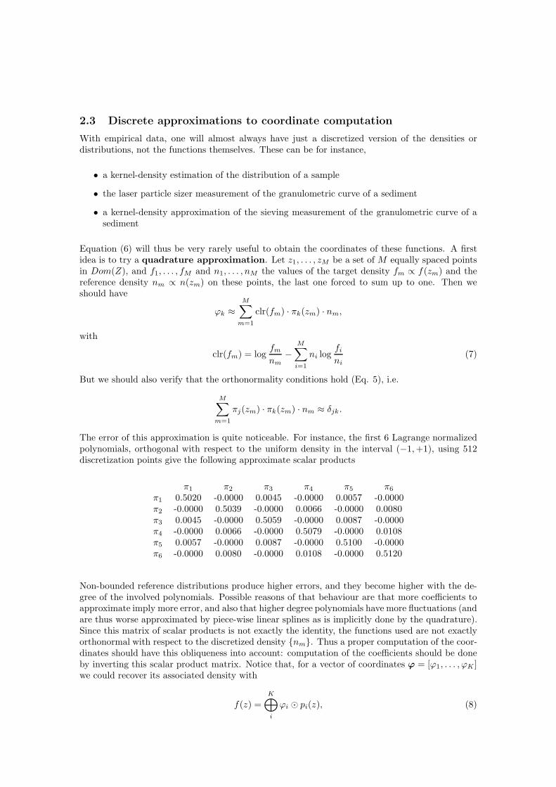
The error of this approximation is quite noticeable. For instance, the first 6 Lagrange normalizedpolynomials, orthogonal with respect to the uniform density in the interval (−1, +1), using 512discretization points give the following approximate scalar products

π1 π2 π3 π4 π5 π6

π1 0.5020 -0.0000 0.0045 -0.0000 0.0057 -0.0000π2 -0.0000 0.5039 -0.0000 0.0066 -0.0000 0.0080π3 0.0045 -0.0000 0.5059 -0.0000 0.0087 -0.0000π4 -0.0000 0.0066 -0.0000 0.5079 -0.0000 0.0108π5 0.0057 -0.0000 0.0087 -0.0000 0.5100 -0.0000π6 -0.0000 0.0080 -0.0000 0.0108 -0.0000 0.5120

Non-bounded reference distributions produce higher errors, and they become higher with the de-gree of the involved polynomials. Possible reasons of that behaviour are that more coefficients toapproximate imply more error, and also that higher degree polynomials have more fluctuations (andare thus worse approximated by piece-wise linear splines as is implicitly done by the quadrature).Since this matrix of scalar products is not exactly the identity, the functions used are not exactlyorthonormal with respect to the discretized density {nm}. Thus a proper computation of the coor-dinates should have this obliqueness into account: computation of the coefficients should be doneby inverting this scalar product matrix. Notice that, for a vector of coordinates ϕ = [ϕ1, . . . , ϕK ]we could recover its associated density with

f(z) =K⊕

i

ϕi ⊙ pi(z), (8)

−15 −10 −5 0 5

050

100

150

mean: −5cl

r−de

nsity

−15 −10 −5 0 5

0.00

0.04

0.08

0.12

var: 10

Den

sity

−5 0 5

05

1015

2025

mean: 0

clr−

dens

ity

−5 0 5

0.00

0.05

0.10

0.15

0.20

var: 4

Den

sity

0 2 4 6 8 10

−10

010

2030

40

mean: 5

clr−

dens

ity

0 2 4 6 8 10

0.00

0.10

0.20

0.30

var: 2

Den

sity

−4 −2 0 2

−4

−3

−2

−1

0

mean: 0

clr−

dens

ity

−4 −2 0 2

0.0

0.1

0.2

0.3

0.4

var: 1

Den

sity

−1.0 −0.5 0.0 0.5 1.0

−8

−6

−4

−2

0

mean: 0

clr−

dens

ity

−1.0 −0.5 0.0 0.5 1.0

0.0

0.2

0.4

0.6

0.8

1.0

1.2

1.4

var: 0.1

Den

sity

2 3 4 5 6 7

−5

05

1015

20

mean: 5

clr−

dens

ity

2 3 4 5 6 7

0.0

0.1

0.2

0.3

0.4

0.5

0.6

var: 0.5

Den

sity

Figure 2: Estimation of coordinates for a normal distribution, with weighted regression (blue), with conventionalregression (green), and with the relationships with the moments (red), applied to a kernel density estimate (black)obtained from the same random sample of size 1000 (for each case, conveniently scaled and translated according tothe variance and mean given in the pairs of plots).

with the vector pi(z) the exponential of the appropiate i-degree polynomial defining the basis. Bymultiplying it with another vector of the basis, one gets

〈f(z), pj(z)〉 =

K∑

i

ϕi · 〈pi(z), pj(z)〉,

Take the vectors of the values of the involved functions on the M discretization nodes, con-veniently clr-transformed through the discete version of (Eq. 3), and denote them by pi =[πi(z1), . . . , πi(zM )] and f = [f∗(z1), . . . , f

∗(zM )], where f∗(zm) = clr(f(zm)). Let us arrangeall pi in a M ×K matrix P. Finally, define weights wm ∝ n(zm) and summing up to one, and ar-range them in a diagonal matrix W. The previous expression with scalar products can be expressedfor all pj(z) simultaneously as

Pt · W · f = Pt ·W ·P · ϕ, (9)

which coincides with the equation of weigthed linear regression, identifying the explanatoryvariables as the polynomials P, and the explained variable as the studied function f . In otherwords, the slight departures from orthonormality shown can be compensated by using weightedlinear regression to estimate the coordinates instead of directly projecting the function onto thebasis in use.

Finally, there is a third way to compute the coordinates, only valid in case of restricting our studyto the classical densities, that is, 2 coordinates for a normal, 1 coordinate for an exponential. Inthis case, the relations between the conventional parameters (mean, variance, scaling) and thecoordinates can be found in Table 1.

Figure 2 compares the results of these two last methods (weighted regression and moment esti-mation), for several combinations of means and variances. The method of plugging the empiricalmoments in the equations for the coordinates provides excellent results (and quickly), but it isnot as interesting (there are other standard ways of comparing normal distributions) and is notvalid for other general cases. On the contrary, weighted regression is extremely sensitive to thelocation parameter of the distribution. Using weights is nevertheless interesting because they focus

the fit on an area around the mean, and downweight the tails, prone to stronger fluctuations.However, the farther the true mean from the origin is, the worse the regression becomes, becausethe “interesting” part of the studied distribution falls in the tail of the reference distribution, thestandard normal density. Here the concept “farther” should be evaluated in a Mahalanobis sense,with respect to the variance of the studied distribution and the reference. In conclusion, it seemsinteresting to allow the reference distribution to be adapted to each particular application. Nev-ertheless, using weighted regression should be done with caution: our experiments (not reportedhere) led us to conclude that the system becomes easily singular, specially when including highorder polynomials.

2.4 Proposed algorithm and R functions

With the preceding theoretical and practical considerations, the following algorithm is proposed tostatistically treat densities. We implemented some of its steps in several functions in R, following theconventions and classes of the package “compositions”(van den Boogaart and Tolosana-Delgado,2008). Given that “density” is an existing object class in R, we generated an Aitchison-geometry-density class under the name of adensity. We created some methods for treating them in thegeneric functions already existing, like cdt and idt (wrappers around clr and ilr transformations),but also some functions specially defined for density treatment. These functions are mentioned inthe following points.

(1). Look at the several densities to be compared, and choose the support where the density will bestudied (minimum and maximum values for z, number of discretization points). To obtain adensity from a data set, use adensity(z), a wrapper on the standard function adensity(z)

for kernel estimation. To obtain a density from sieving data, use sieve2adensity (witharguments x= sieve φ values and y= mass on each sieve).

(2). Choose a reference distribution, the highest degree of the polynomials, and a scaling of thesupport (function gsi.ilrBase.adensity does it explicitly, but idt.adensity calls this oneimplicitly):

(2.1) the reference density can be a normal, an exponential and an uniform one

(2.2) the highest degree K must be even for the normal case, and can be freely chosen for theother two

(2.3) the scaling

z∗ =z − a

b

of the support is aimed at adequately focusing the reference distribution, and it can bedone automatically to ensure that the reference density has only a probability α=alpha

outside the support:

a b

normal min(z)+max(z)2

max(z)−min(z)2qα/2

exponential min(z) max(z)−min(z)qα

uniform min(z)+max(z)2

max(z)−min(z)2 .

Here qα represents the α quantile of a standard normal or an exponential distribution(with λ = 1).

(3). Compute the coordinates of each density with respect to the chosen basis (idt.adensity),with the following sub-steps:

(3.1) scale the support as mentioned before (and use z∗ from now on),

(3.2) remove those nodes where the discretized density is zero,

(3.3) obtain the weights wi as proportional to the reference density evaluated at the remainingnodes, and summing up to one

(3.4) apply the clr transformation for a discretized density (Eq. 7) using the weights wi

instead of ni,

(3.5) use weighted regression (Eq. 9) to explain the clr-transformed density as a linear com-bination of the first K + 1 orthonormal polynomials with respect to the chosen density(non-weighted regression is used instead if the optional argument weighted=FALSE isgiven to idt.adensity),

(3.6) remove the coefficient of the constant; the remaining coefficients are the estimates ofthe coordinates (an object of class adensity.rmult).

(4). Apply the desired statistical method to the coordinates.

(5). For those results describing a density, apply the coordinates to the basis to recover thatdensity (idt.inv.adensity.rmult to obtain a adensity object, or lines.adensity.rmultto plot it). This is done as follows:

(5.1) at all M scaled nodes, evaluate the orthonormal polynomials (not including the constantπ0(z

∗) ∝ 1)

(5.2) multiply the polynomials by the coefficients

(5.3) add the logarithm of the reference density evaluated at the nodes

(5.4) take exponentials,

(5.5) rescale the support, to recover the original z = a + b · z∗(5.6) close the resulting discretized density to sum up to one, conveniently weighted by the

node interdistance (max(z) − min(z))/(M − 1), as would correspond with a histogram.

3 Applications

3.1 Sand size distribution of the Darss Sill

This example deals with a typical reference data set of grain size problems: the Darss sill dataset. The Darss Sill is situated between the Danish isles of Falster and Møn in the northwest andthe Darss peninsula in Germany in the southeast, at the entrance of the Baltic Sea. Lemke (1997)reports the main geologic and physiographic conditions controlling the distribution of sediment onthis structure. The data set contains 1281 sandy surface samples, which were dried and sieved intoeight weight-percent size fractions, from less than 63 µm (silt and finer) to over 2000 µm (graveland coarser).

This data set was the focus of a session in IAMG’97 (Pawlowsky-Glahn, 1997), where reseacherspresented several approaches. Among them, two are linked to the approach of this contribution,though in different ways. Martın-Fernandez et al. (1997) took the eight grain size categories asparts of a composition, amalgamated four of them (from gravel to medium sand) and applied theadditive log-ratio transformation to the resulting 5-part composition, after a zero substitution ofthe remaining zero components. These log-ratio transformed values were the data to a parametricclassification scheme, generating 7 groups. On the other hand, Tauber (1997) suggested to treatthem as a continuous distribution, and fitted an analytic approximation of the normal cdf to theempirical cdf of the grain size. This analytic function depended on a location parameter (median)and a scale parameter (sorting). These two parameters were then used as “data” in the subsequentanalysis (clustering, regionalization, etc.), concluding that the grain size distributions showed morea continuous pattern than groups.

Both approaches have interesting advantages and some inconvenients. The log-ratio approachrequires amalgamation and zero substitution, which respectively removes some important sedi-mentologic information and generates spurious clusters (Tauber, 1999). But the median-sorting

−20000 0 20000 40000 60000 80000 100000

4180

000

4190

000

4200

000

4210

000

4220

000

4230

000

4240

000

Easting

Nor

thin

g

µ σ2

−2; −3−1; −20; −11; 02; 13; 24; 35; 46; 57; 68; 79; 810; 911; 1012; 1113; 1214; 13

siltnon−normalnormal

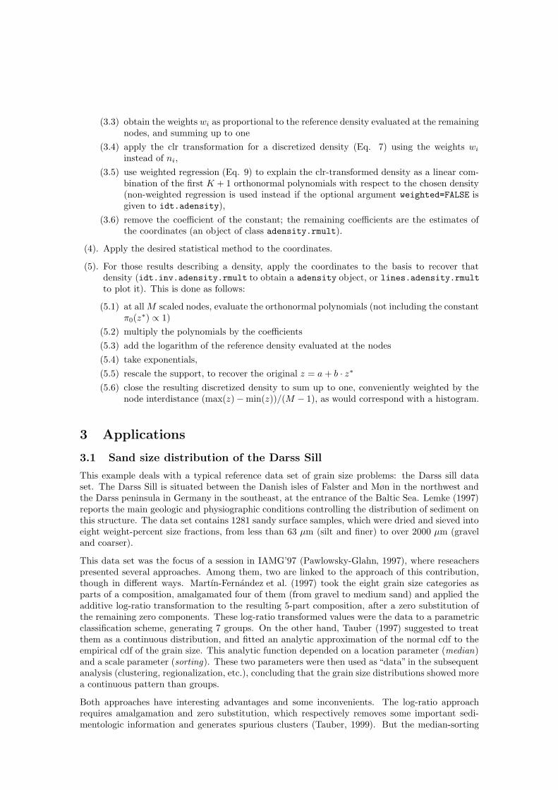
Figure 3: Map of the first coordinate of the grain size distribution of the Darss sill samples (Baltic Sea). Silt samplesare singularized with green circles (correspond to groups 8 and 9 of non-normal samples). Most of the samplesadmitted a representation with k=2 (labelled as “normal”), whereas some few present important skewness/kurtosis(labelled as “non-normal”; for them, the expression of the first coordinate as a function of the moments is not valid).

approach is limited to normal distributions, and would yield very different results if we change theparametrization of the curve, which in the end is something arbitrary; e.g. we could work withstandard deviation instead of sorting (they are proportional for normal curves), with variance, withtheir inverses or with their logarithms. Any of these parametrizations is valid and meaningful in acontext, but they would not lead to the same results. In contrast, Martın-Fernandez et al. (1997)is “non-parametric”, and can incorporate non-normal distributions. Nevertheless, both approachesare “spurious-correlation-free”.

The approach proposed in this contribution builds a bridge beween them: we found that bygeneralizing the log-ratio approach to continuous densities, the two first coordinates to describea normal distribution provide a “natural” parametrization. The euclidean distance between thesecoordinates is (approximately) isometric to the log-ratio distance compatible with the Hilbert spacestructure [Eqs. (2-4)]. And if one has non-normal distributions (skew or kurtotic), adding morecoordinates one can describe them in the same consistent way. Moreover, we do not need to replacezeroes of the composition, as they are removed in step (3)3.2 from the computation.

To treat the data (previously recasted to a density by sieve2adensity function), we used a normaldistribution as reference, scaled between φ -4 and 7 (probability 1% outside this interval), and k = 4Hermite polynomials as basis. Most of the curves, nevertheless, were not satisfactorily describedwith four coordinates, as the last one got a positive coefficient (i.e., they would not be boundeddensities). Therefore, for them we switched to k = 2, thus a normal distribution actually: theseare mapped in Figure 3, by using the first coordinate, which is a sort of coefficient of variation(Table 1).

For those “non-normal” data, a Ward cluster analysis was used to try to find similar patterns ofdeviation from normality. The dendrogram of Figure 4 shows the dendrogram, and Figure 5 thespatial distribution of each cluster. This last figure also shows the several grain size curves of eachgroup and their average. This average is the grain size curve having as parameters the average ofthe parameters of the curves within the group.

The first group suggests bimodality, a mixture of fine sand and clay/silt (with missing very find

687756

658768

780720757633637694

510766

3995473518976093285578335833505258668525447283726824932462521185911

1183686184752847907

112111373264684627771182784

1317853

11361162

204381

131311451157

678827892

11681310405806202581167124553162552556655423592487

116416185622322622154674162464192777

419145

13071316101

1308201296543755638142599224228512

1043593

1019157579121173725765864824848689801

40788199235200535

0 20 40 60 80 100

ward m

ethod

height

Fig

ure

4:

Den

dro

gra

mofW

ard

cluster

analy

sisofth

enon-n

orm

algra

insize

curv

es.N

ote

that

the

vertica

lsca

leis

represen

tedas

itssq

uare

root.

020000

4000060000

80000

4180000 4200000 4220000 4240000

020000

4000060000

80000

4180000 4200000 4220000 4240000

020000

4000060000

80000

4180000 4200000 4220000 4240000

020000

4000060000

80000

4180000 4200000 4220000 4240000

020000

4000060000

80000

4180000 4200000 4220000 4240000

020000

4000060000

80000

4180000 4200000 4220000 4240000

020000

4000060000

80000

4180000 4200000 4220000 4240000

020000

4000060000

80000

4180000 4200000 4220000 4240000

020000

4000060000

80000

4180000 4200000 4220000 4240000

Fig

ure

5:

The

9gro

ups

ofnon-n

orm

algra

insize

curv

es.For

each

gro

up,th

esp

atia

ldistrib

utio

nis

show

n(m

ain

plo

t),as

well

as

the

φdistrib

utio

nofall

the

data

,to

geth

erw

ithth

eav

erage

distrib

utio

n(th

at

one

with

coord

inates

the

avera

ge

with

inth

egro

up).

sample RT1− 2

Den

sity

0 5 10 15

0.00

0.05

0.10

0.15

0.20

0.25

0.30

0.35

sample RT1− 7c

Den

sity

0 5 10 15

0.00

0.05

0.10

0.15

sample RT1− 8

Den

sity

0 5 10 15

0.00

0.05

0.10

0.15

0.20

0.25

0.30

0.35

sample RT1− 9

Den

sity

0 5 10 15

0.0

0.1

0.2

0.3

sample RT1− 16

Den

sity

0 5 10 15

0.0

0.1

0.2

0.3

0.4

sample RT1− 19

Den

sity

0 5 10 15

0.00

0.05

0.10

0.15

0.20

Figure 6: Grain size measurements of four sediment samples, with two techniques: laser particle sizer (blue linesfor each of the 5 measurements, gray area for their average), and sieving plus centrifugation-settling (histogram).The red line represents the estimated reconciled curve.

sand). The second and third groups are fine sands, with asymmetry to the right and the leftrespectively. The fourth group is very similar to the third, but with a sharper lack of mediumsand. The fifth and the second are also very similar, though the second is clean of coarser sandcategories which occur in the fifth. The sixth and seventh are unclear groups, with very differentdistributions respectively showing kurtotic and skew averages. Finally the eigth and ninth groupsare silt-rich samples, where the method (focusing on the sand domain as it does) failed to correctlyfit a curve, and identified a very fine sand mode and a silt mode: these samples are better leftbehind.

3.2 Reconciling measurements from different methods

In this application, the problem is to take two sets of measurements of the grain size curve,with different support, different precision and different optimal domains, and try to find a globalgrain size curve accounting for all this information. In the present case (Fig. 6), we have LPSmeasurements in the range φ ∈ [−1, 14.61] split in 116 equally-spaced classes, and another set ofcombined sieving/settling measures covering the range φ ∈ (−2, 8) in units plus a last residual classfor grain sizes in [8,∞). Let us denote these two sets of supports (classes) as {xi, i = 1, . . . , 116} and{yi, i = 1, . . . , 11}, and the proportion of grains falling in each class as {fi = f(xi), i = 1, . . . , 116}and {gi = g(yi), i = 1, . . . , 11}.

The idea is to find a curve like (8), which lies at a minimum average distance from both LPS and

−5 0 5 10 15

φ

−5 0 5 10 15

−2

−1

01

2

φ

Figure 7: (left) Comparison of the three possible reference curves, scaled to contain at least 99% of probability inthe sampled domain. (right) Scaled Legendre orthonormal polynomials used in this example.

sieving/settling measurements. The first step is to choose a reference distribution, giving weightsto each xi or yi, thus it can incorporate our knowledge on which methods are optimal for whichsubdomains of the φ spectrum. For instance, we know that LPS data from the right part of φshould not be trusted: if we take an exponential reference, the result would be the opposite, asthose are just the points where the exponential density is higher (see Fig. 7). Both the normaldistribution and the uniform could be reasonable choices. In this case, we take the uniform, to befairer with the sieving/settling data against the LPS.

Then we use k = 10 Legendre polynomials Lk(x), orthonormal with respect to the uniform distri-bution. By evaluating each of them at the sampling nodes, xi and yi, we obtain k + 1 explanatoryvariables (including the constant L0(x) ≡ 1), used in a weighted linear regression procedure toexplain the clr-transformed values of {fi} and {gi}. Regarding the constant, remember that itscoefficient (the intercept) will be ignored, as it just ensures a sum of zero for this particular clrvalues: in other words, each of the two data sets should be allowed to have different interceptsbut the same coefficients. This is readily obtained by adding another explanatory variable equalto zero for xi and to one for yi. And if we had more methods to reconcile, we would add one ofthese auxiliary intercepts for each of them. The final system is thus:

0 1 L1(x∗1) · · · Lk(x∗

1)0 1 L1(x

∗2) · · · Lk(x∗

2)...

......

. . ....

0 1 L1(x∗116) · · · Lk(x∗

116)1 1 L1(y

∗1) · · · Lk(y∗

1)1 1 L1(y

∗2) · · · Lk(y∗

2)...

......

. . ....

1 1 L1(y∗11) · · · Lk(y∗

11)

︸ ︷︷ ︸

P

·

ϕ′0

ϕ0

ϕ1

...ϕk

︸ ︷︷ ︸

ϕ

= ln

f1

f2

...f116

g1

g2

...g11

︸ ︷︷ ︸

f

,

with the following practical comments:

• the support points are rescaled following step (2)2.3 of the general procedure (page 9);

• each points from a LPS measurement has the same weight; to give the sieving/settling dataa similar influence while capturing the asymmetry in the reliability of the sieves, we give thefirst sieve a weight of 2.5×11, the second a weight of 2.5×10, etc., and the eleventh categorya weight of 2.5× 1; this amounts to giving LPS a total weight of 116 and to sieving/settling2.5 × 65

0 5 10 15

−6

−4

−2

02

4

2

clr−

dens

ity

0 5 10 15

−5

−4

−3

−2

−1

01

7c

clr−

dens

ity

0 5 10 15

−4

−2

02

8

clr−

dens

ity

2 4 6 8 10 12 14

−4

−2

02

9

clr−

dens

ity

0 5 10 15

−8

−6

−4

−2

02

16

clr−

dens

ity

0 5 10 15

−6

−4

−2

02

19

clr−

dens

ity

Figure 8: Grain size measurements of four sediment samples, expressed in clr scale, but normalized to the sameupper value (instead of to zero sum), in order to enhance the comparison of the three data sets. Big circles correspondto data coming from sieving/settling, and small circles to data from LPS. Their areas are proportional to the weightsgiven to each point. The red line represents the estimated reconciled curve, obtained with Legendre polynomials ofhighest degree (from left to right, top to bottom): 10, 6, 6, 8, 8, 10.

• if some of the fi or gi are zero, the corresponding row of both P and f matrices is erased andthe weights reclosed;

• if one is using a reference density n(x) different from the uniform one, each fi and gi mustbe replaced by their relative densities, namely fi/n(x∗

i ) and gi/n(x∗i ).

The result is shown as a red line in both Figures 6 and 8, respectively showing the original fi andgi and their clr-transformed values, together with the resulting fitted model.

3.3 Cr-spinel distribution “facies”

Spinel is a part of a quite continuous series of igneous isometric/cubic minerals with formula XY2Oa

where X is bivalent (Fe2+, Mg or Mn) whereas Y is typically trivalent (Al3+, Cr3+, Ti4+ andFe3+). Actual spinel composition depends on its host rock, a fact that gave rise to its widespreaduse as a petrogenetic indicator mineral (see Barnes and Roeder, 2001, for a review). In mantlerocks, such as peridotites, spinel Ti<0.2 wt% (Kamenetsky et al., 2001), and the Cr/Al ratio isan approximative measure of the degree of partial melting the rocks underwent. Cr/Al ratiosare thus low in lherzolites and high in the more depleted harzburgites (Dick and Bullen 1984).Spinel crystallized from magmatic melts has typically TiO2 >0.2 wt%. Such rocks constitutethe majority of ophiolite suites, which play an important role in establishing tectonic models formountain building; both directly, and indirectly through the study of detrital spinels in sedimentsderived from the ophiolites. Interest will be in this case to compare the empirical distributionsof the proportions of the major end member molecules FeCr2O4 and MgAl2O4 of detrital Cr-spinel. The samples represent several Alpine basins in the Dinaride and Carpathian mountainbelts. The goal of the approach is to reveal similarities between samples, which might be deemedas “probability-facies”and possibly be used to derive the relative contributions of each of the threerock types to the sediment.

Traditional analysis of Cr-spinel grains is done on the space of the so-called Mg-index vs. Cr -index,these are the proportions of Mg in {Mg, Fe2+} subcomposition and the proportion of Cr in {Cr, Al}(Fig. 9). In this space, most of the data fall on the diagonal between the end-member moleculesFeCr2O4 and MgAl2O4, due to the fact that a significant amount of chemical variation in mostCr-spinels can be readily described in terms of these two molecules alone. At this stage, low-Ti(mantle) and high-Ti (magmatic) spinels need to be treated separately, due to their different origin(Barnes and Roeder, 2001; Kamenetsky et al., 2001).

Due to the petrogenetic significance of the Mg+Cr ↔ Fe2++Al cation substitution, our data areprojected onto this exchange line, and we work with the variable:

x =

CrCr+Al

+ FeFe+Mg

2.

This is applied a logit transformation, and a kernel density estimation is used for all grains comingfrom the same tectono-stratigraphic unit, after removing the outliers from each of them. In thisway, 41 densities are obtained, and then each one is expressed in k = 10 coordinates with respectto a normal distribution and Hermite polynomials. This procedure is applied only to the low-Tispinels (mantle). At this point, 3 samples were removed due to their extreme character (“BosnianFlysch / Ugar”, “X-Kruja / ALB” and “XN-Krk ML”). To account for the high-Ti (magmatic)spinels in the remaining samples, we derive the proportion of cristals with high Ti from each unit,compute its logit transformation and rescale the result, in order to give it the same standarddeviation as the average of the 10 coordinates of the low-Ti part. This provides a data set with 11variables and 38 cases.

A Ward cluster analysis (Fig. 10) revealed two main groups, two small groups and 2 atypicalsamples (apart from those 3 removed from the beginning)

Fe2−i

Cr−

i

0.0 0.2 0.4 0.6 0.8 1.0

0.0

0.2

0.4

0.6

0.8

1.0

1.0 0.8 0.6 0.4 0.2 0.0

Mg−i

1.0

0.8

0.6

0.4

0.2

0.0

Al−

i

Figure 9: Distribution of Cr-spinel single grain compositions, for high-Ti (red, > 0.2%) and low-Ti (black, ≤ 0.2%)crystals. Contours are isodensity curves enclosing 50, 75, 90 and 95% of the data. The density was obtained usinga 2D-kernel estimation in the logit-logit transformed space.

Bük

k

X−

SA

Z (

Kru

ja)

/ ?B

udva

−C

ukal

i

Viv

odin

a

XN

−P

Z

XN

−V

P

Glo

g

N P

indo

s M

ts. B

osni

an F

lysc

h?

VZ

− W

−T

rebo

vac

Kra

vlja

k

X−

Pag

VZ

− M

ajev

ica

Bos

nian

Fly

sch

/ Vra

nduk

W−

Car

p

X−

ND

, Rav

ni−

Kot

ari

XN

−T

K

X−

SA

Z

Ger

ecse

Bis

tra

X−

Dal

mH

erz

Ost

rc

X−

Kru

ja [w

indo

w] /

ALB

N P

indo

s M

ts.

DO

Z −

Cac

ak−

Nov

i Paz

ar fa

n

XN

−K

rk

XN

−B

K

Pci

nja

Gro

up

XN

−G

B

VZ

− V

ucja

k

X−

Ioni

an, A

LB

VZ

− K

ozar

a

X−

CD

, Spl

it ar

ea XN

−R

ab

Ovc

e P

ole

Gro

up

X−

CD

, S o

f Spl

it

VZ

− L

jig

X−

SA

Z (

Bud

va?)

DO

Z m

elan

ge

Pog

ari F

m.0

5010

015

020

0ward

Hei

ght

Figure 10: Cluster analysis of the stratigraphic units, using the coordinates of the distribution of FeCr2O6 vs.MgAl2O6 proportion, as well as the proportion of low-Ti to high-Ti grains (in log scale). Three samples (“BosnianFlysch / Ugar”, “X-Kruja / ALB”and“XN-Krk ML”) were completely removed, due to its extreme outlying character.

−1.5 −1.0 −0.5 0.0 0.5 1.0 1.5

0.0

0.5

1.0

1.5

N = 123 Bandwidth = 0.1478

Den

sity

group 1

−1.5 −1.0 −0.5 0.0 0.5 1.0 1.5

0.0

0.2

0.4

0.6

0.8

1.0

1.2

N = 59 Bandwidth = 0.1854

Den

sity

group 2

−1.5 −1.0 −0.5 0.0 0.5 1.0 1.5

0.0

0.5

1.0

1.5

Bükk

Den

sity

34.1

−1.5 −1.0 −0.5 0.0 0.5 1.0 1.5

0.0

0.5

1.0

1.5

2.0

2.5

N = 16 Bandwidth = 0.1094

Den

sity

group 4

−1.5 −1.0 −0.5 0.0 0.5 1.0 1.5

0.0

0.5

1.0

1.5

2.0

2.5

N = 77 Bandwidth = 0.1158

Den

sity

group 5

−1.5 −1.0 −0.5 0.0 0.5 1.0 1.5

0.0

0.5

1.0

1.5

X−SAZ (Kruja) / ?Budva−Cukali

Den

sity

14.5

−1.5 −1.0 −0.5 0.0 0.5 1.0 1.5

0.0

0.5

1.0

1.5

2.0

2.5

Bosnian Flysch / Ugar

N = 57 Bandwidth = 0.07393

Den

sity

28.1

−1.5 −1.0 −0.5 0.0 0.5 1.0 1.5

0.0

0.5

1.0

1.5

2.0

2.5

X−Kruja / ALB

N = 65 Bandwidth = 0.06321

Den

sity

40.9

−1.5 −1.0 −0.5 0.0 0.5 1.0 1.5

0.0

0.5

1.0

1.5

2.0

2.5

3.0

XN−Krk_ML

Den

sity

31.3

12

34

56

78

9

10 20 30 40 50

Figure 11: Characterization of the several groups (and single atypical samples) obtained with cluster analysis of thestratigraphic units. For each group, the kernel density estimates of all the samples is represented in grey, and theiraverage (in the coordinate scale) is portrayed in red. For each atypical sample, we represent the kernel density andits coordinate simplification, together with the data set (as a rug in the x axis) and the proportion of high-Ti crystalsin the sediment (number at the upper left corner, in %). Finally a box-plot of these high-Ti crystal proportions foreach group is also included.

In basins with ophiolitic detritus, provenance of Cr-spinel grains has been traditionally assessedmainly using the range of Cr in the (Cr, Al)-subcomposition, the TiO2 content, and the calculatedFe3+/Fe2+ ratio, by visual estimation from discrimination diagrams. However, Alpine ophiolitecomplexes are petrologically often extremely inhomogeneous on a map scale (Dick and Bullen,1984), which is also reflected by the composition of spinels they would release into the sediment.Obduction and subsequent tectonics may further rearrange individual spinel-bearing magmatic andmantle-derived members of the ophiolite suite. Upon tapping by the drainage system, sedimentcomposition will thus largely depend on this previous history of the ophiolite suite. Distributionof detrital Cr-spinel chemical parameters therefore reflects the net effect of oceanic litosphericevolution, obduction, subsequent tectonics and the extent of the drainage, rather than the“ophiolitetype” alone. We propose that comparison of sediments should rely on the integrative examinationof the useful parameters as presented here. We suggest that any similarity between samples isnot necessarily an indication of “palaeogeographic connection” but simply a result of a similarsedimentary response whenever the above evolutionary steps share a common history.

The significance of our approach is twofold. Results reveal that, first, several stratigraphic units,previously tentatively correlated based on geographic proximity, age, lithofacies and tectonic con-siderations, indeed received detritus of quite similar “final” composition. For example, similaritybetween the units DOZ melange and Pogari Fm., as well as between the Gerecse, Ostrc and Bistraformations, is corroborated by field and stratigraphic relations. Also, the observed dissimilaritybetween the DOZ melangee and Vranduk are supported by independent geological data.

Second, there are notable differences between some stratigraphic units in the cluster dendrogram(Fig. 10), though they were previously considered as “related” based on some of the above cri-teria. An evaluation of this technique usefulness to sediment provenance analysis still presentssome “geologic” caveats, being the role of the Ti-threshold an important one. For example, let usassume that the units “X-CD, S of Split” and “X-CD, Split area” are related, based on the similarcompositional range of their low-Ti spinels, and the position of local maxima of the polynomialfunctions, both being around -1 and -0.2 (in logit scale). It is possible that a choice of the TiO2

threshold different from the actual one would result in a different data distribution. In other words,coordinates of the variation of Mg in the (Fe2+, Mg)-subcomposition, being similar to the Fe-Titrend of Barnes and Roeder (2001), should also be included in the cluster analysis in future.

The distribution of Ti-rich and Ti-poor spinels in the units, shown in conjunction with the clusteranalysis results illustrates the importance of the distribution alone on the eventual separation of theunits (Fig.11). For example, groups 1 and 2, the members of which having small Ward distances,differ in the ranges of their logit Ti-functions. A possible interpretation of this pattern is thatunits in group 2 were supplied by detritus from an ophiolitic source where a higher proportionof magmatic units were subject to erosion, while the composition of the mantle-derived memberswas comparable for both units. It is recalled that obducted ophiolites are typically dissected alongpetrological boundaries, thus pursuing this approach may add considerable precision to source areaassignment and tectonic reconstructions in future.

4 Closing remarks

This work is a preliminary yet promising application to the theory of “continuous compositions”de-veloped by Egozcue and Dıaz-Barrero (2003); Egozcue et al. (2006) and van den Boogaart (2005).The main goal is to compare the distribution of a given property in batches of grains (or crystals)from several sediment bodies (or rocks), and infer relations of evolution, proximity, distance, etc.,between the sediment bodies (or rocks). As one deduces an “electrofacies” or a “petrofacies” fromthe electric-logged characteristics or the petrographic composition of a sediment/rock, we proposeto define some sort of “densofacies” of the studied property as a descriptor of that sediment/rock

This is done in the following steps:

(1). choice of a (discretized) support for the desired property;

(2). estimation though kernel techniques of its density on that domain;

(3). division of the density by an adequate, scaled reference density (normal, exponential oruniform);

(4). regression of that relative density in log scale (completely removing nodes with estimatedzero density) against some polynomials orthonormal with respect to the reference density(respectively Hermite, Laguerre or Legendre polynomials). This regression may be weightedusing weights proportional to the reference density chosen.

The obtained regression coefficients (removing the coefficient-intercept) are adequately scaled withrespect to each other, and characterize the density in a compact way, thus they can be used as inputfor further statistical treatment (covariance-based or distance-based). In the language of Hilbertspaces, these coefficients are estimates of the coordinates of the studied density with respect to thebasis integrated by the (exponentiated) polynomials used.

There are many properties of single grains/crystals that can be treated in this way, though themost commonly measured one is its size/volume: this gives granulometric curves, one of the mostinformative characteristics of a sediment when studying its originating erosion, transport anddeposition processes. For this particular case, an interesting application presented here is thecompatibilization (a sort of “averaging”) of grain size curves of the same sediment obtained withdifferent measuring techniques. As a side result, we have also found that the “best” 2 parametersof a normal distribution in this framework are linearly related to the natural parameters of thecorresponding exponential family (µ/σ2 and (1/σ2 − 1)/

√2).

5 Acknowledgements

This research was funded by the the German Research Foundation (DFG, grant EY23/11-1) and theDepartment of Universities, Research and Information Society (DURSI, grant 2005 BP-A 10116)of the Generalitat de Catalunya. The authors are also very grateful to the fruitful discussions withJ.J. Egozcue and V. Pawlowsky-Glahn.

REFERENCES

Barnes, S. and P. Roeder (2001). The range of spinel compositions in terrestrial mafic and ultra-mafic rocks. Journal of Petrology 42 (12), 2279–2302.

van den Boogaart, K. (2005). Statistics structured by the Aitchison Space. In G. Mateu-Figuerasand C. Barcelo-Vidal (Eds.), Compositional Data Analysis Workshop – CoDaWork’05, Proceed-ings. Universitat de Girona, ISBN 84-8458-222-1, http://ima.udg.es/Activitats/CoDaWork05/.

van den Boogaart, K. G. and R. Tolosana-Delgado (2008). “compositions”: a unified R package toanalyze Compositional Data. Computers and Geosciences 34 (4), 320–338.

Dick, H. and T. Bullen (1984). Chromian spinel as a petrogenetic indicator in abyssal and alpine-type peridotites and spatially associated lavas. Contributions to Mineralogy and Petrology 86 (1),54–76.

Egozcue, J. J. and J. L. Dıaz-Barrero (2003). Hilbert space on probability density functions withAitchison geometry. In S. Thio-Henestrosa and J. A. Martın-Fernandez (Eds.), CompositionalData Analysis Workshop – CoDaWork’03, Proceedings. Universitat de Girona, ISBN 84-8458-111-X, http://ima.udg.es/Activitats/CoDaWork03/.

Egozcue, J. J., J. L. Dıaz-Barrero, and V. Pawlowsky-Glahn (2006). Hilbert space of probabilitydensity functions based on Aitchison geometry. Acta Mathematica Sinica (English Series) 22 (4),1175–1182. DOI: 10.1007/s10114-005-0678-2.

Kamenetsky, V., A. Crawford, and S. Meffre (2001). Factors controlling chemistry of magmaticspinel; an empirical study of associated olivine, cr-spinel and melt inclusions from primitiverocks. Journal of Petrology 42 (4), 655–671.

Lemke, W. (1997). The Darss Sill in the southwestern Baltic sea – hydrographic and geologicalsetting. See Pawlowsky-Glahn (1997), pp. 135–138.

Lwin, T. (2003). Parameterization of particle size distributions by three methods. MathematicalGeology 35 (6), 719–736.

Martın-Fernandez, J. A., C. Barcelo-Vidal, and V. Pawlowsky-Glahn (1997). Different Classi-fications of the Darss Sill Data Set Based on Mixture Models for Compositional Data. SeePawlowsky-Glahn (1997), pp. 151–156.

McLaren, P. and D. Bowles (1985). The effects of sediment transport on grain-size distributions.Journal of Sedimentary Petrology 55 (4), 457–470.

Pawlowsky-Glahn, V. (Ed.) (1997). Proceedings of IAMG’97 — The third annual conference of theInternational Association for Mathematical Geology, Volume I, II and addendum. InternationalCenter for Numerical Methods in Engineering (CIMNE), Barcelona (E), 1100 p.

Sircombe, K. N. (2000). Quantitative comparison of large sets of geochronological data usingmultivariate analysis: A provenance study example from Australia. Geochimica et CosmochimicaActa 64 (9), 1593–1616.

Tauber, F. (1997). Treating grain-size data as continuous functions. See Pawlowsky-Glahn (1997),pp. 169–174.

Tauber, F. (1999). Spurious clusters in granulometric data caused by logratio transformation.Mathematical Geology 31 (5), 491–504.