Embed Size (px)
Citation preview
DOI: 10.1007/s10909-006-9219-3Journal of Low Temperature Physics, Vol. 143, Nos. 5/6, June 2006 (© 2006)
Statistical Theory of Spin Relaxation and Diffusionin Solids
A. L. Kuzemsky
Bogoliubov Laboratory of Theoretical Physics, Joint Institute for Nuclear Research,141980 Dubna, Moscow Region, Russia.
E-mail: [email protected]
(Received February 21, 2006; revised May 19, 2006)
A comprehensive theoretical description is given for the spin relaxation anddiffusion in solids. The formulation is made in a general statistical-mechan-ical way. The method of the nonequilibrium statistical operator (NSO)developed by Zubarev is employed to analyze a relaxation dynamics of aspin subsystem. Perturbation of this subsystem in solids may produce anonequilibrium state which is then relaxed to an equilibrium state due tothe interaction between the particles or with a thermal bath (lattice). Thegeneralized kinetic equations were derived previously for a system weaklycoupled to a thermal bath to elucidate the nature of transport and relaxa-tion processes. In this paper, these results are used to describe the relaxa-tion and diffusion of nuclear spins in solids. The aim is to formulate a suc-cessive and coherent microscopic description of the nuclear magnetic relaxa-tion and diffusion in solids. The nuclear spin–lattice relaxation is consideredand the Gorter relation is derived. As an example, a theory of spin diffusionof the nuclear magnetic moment in dilute alloys (like Cu–Mn) is developed.It is shown that due to the dipolar interaction between host nuclear spinsand impurity spins, a nonuniform distribution in the host nuclear spin systemwill occur and consequently the macroscopic relaxation time will be stronglydetermined by the spin diffusion. The explicit expressions for the relaxationtime in certain physically relevant cases are given.
KEY WORDS: Transport processes; nonequilibrium statistical operator;kinetic equation; spin temperature; nuclear spin relaxation and diffusion;dilute alloys.
1. INTRODUCTION
For many years there has been considerable interest, experimentaland theoretical, in relaxation processes occurring in various spin systems,
213
0022-2291/06/0600-0213/0 © 2006 Springer Science+Business Media, Inc.
214 A. L. Kuzemsky
especially the nuclear spin systems in solids and liquids.1–38 In ordinary spinresonance experiments, spins are subject to an applied magnetic field h0 andmake a precessional motion around it. Local fields produced by interactionsof the spins with their environments act as relatively weak perturbations tothe unperturbed precessional motion. In quantum-mechanical language, theexternal field gives rise to the Zeeman levels for each spin and the interac-tions are perturbations to these quantum states. In a nuclear-magnetic reso-nance (NMR) experiment, the nuclear spin system absorbs energy from theexternally applied radio-frequency field and transfers it to the thermal bathor reservoir provided by the lattice through the spin lattice interaction. Thecoupled nuclear spins in a solid with very slow spin–lattice relaxation time T1comprise a quasi-isolated system which for many purposes can be treatedby thermodynamic methods. The spin–spin relaxation time is denoted byT2. The other system, called the lattice, contains all other degrees of free-dom, phonons, translational motion of conduction electrons, etc. It is at atemperature T that it is considered stable. A macroscopic approach to thedescription of magnetic relaxation was proposed by Bloch.3 He proposeda phenomenological equation describing the motion of nuclear-spin systemsubjected to both a static and a time varying magnetic field
d �Mdt
=γ �M× �h−Mx
T2�i−My
T2�j +M0 −Mz
T1�k,
where the external field �h is taken to be of the form �h=h0�k+2h1(t)cosωt�i.This equation successfully describes a wide variety of magnetic resonanceexperiments, although to obtain a valid description of low-frequency phe-nomena, it is necessary to modify the original equation so that relaxationtakes place toward the instantaneous magnetic field. In an NMR experi-ment, the absorption of energy from the applied rf field produces eitheran increase in the energy of the spin system or a transfer of energy fromthe spin system to the lattice. The latter process requires a time intervalof the order of spin–lattice relaxation time T1. The characteristic time T2determines the relaxation of the transversal spin components due to thespin–spin interactions.
The relaxation processes in spin systems have been investigated by a num-ber of authors8,14,20–23,25–28,33,37 to obtain qualitative and quantitative infor-mation about irreversible spin–spin and spin-lattice processes in spin systems.The method of many of these papers was to develop an equation of motionfor the reduced density matrix12,13,16,17 describing the spin system, and wasfound to be most useful when the perturbation responsible for the relaxationof the spin system had a very short correlation time. In the equation-of-motionapproach, the specification of the initial conditions involves the assumption of
Statistical Theory of Spin Relaxation 215
some explicit form for the density matrix describing the system (the systemincludes both the spin and its surroundings, which in the case studied belowwill be the conduction electrons in a metal). This problem is very attractive fromthe point of view of irreversible statistical mechanics since a general model ofmagnetic resonance consists of a driven system of interest in interaction with aheat bath. Stenholm and ter Haar18 have analyzed the basic assumptions whichare necessary for statistical-mechanical derivation of the Bloch equation andthe role of the thermal bath.
An important concept in the interpretation of spin-lattice relaxation phe-nomena was provided by the thermodynamic theory of Ref. 1. They consid-ered the magnetic crystal to be composed of two subsystems, which could beassigned two different temperatures. One subsystem contained the magneticdegrees of freedom. The other subsystem, called the lattice, contains all otherdegrees of freedom. Then, the idea of spin temperature was extended and sev-eral distinct temperatures for magnetic subsystems (Zeeman, dipole–dipole,etc.) were introduced.32 (Note, however, some special exclusions.39) In gen-eral, the state of the total system to be composed of a few subsystems may bedescribed approximately by a density matrix of the form
ρ∼ exp[−(H1/kT1)− (H2/kT2)− (H3/kT3) . . . ]
with a number of quasi-invariant energiesT r(Hi) and a number of distributionparameters T −1
i . Nuclear relaxation in weak applied fields was first treated byRedfield9 and Hebel and Slichter,10 using the idea of spin temperature. Redfieldtheory is the semiclassical density operator theory of spin relaxation.
It was Bloembergen5 who first formulated that the magnetization ofspins in a rigid lattice could be spatially transported by means of the mutualflipping of neighboring spins due to dipole–dipole interaction. This ideapermitted one to explain the significant influence of a small concentrationof paramagnetic impurities on spin–lattice relaxation in ionic crystals. Heused a quantum-mechanical treatment ( first-order perturbation theory) andshowed that the transport equation for magnetization was a diffusion equa-tion. In this simple approximation he calculated the diffusion constant D.In other words, we can roughly represent the relaxation dynamics as
∂〈I z(�r)〉∂t
= −A(�r)[〈I z(�r)〉−〈I z(�r)〉0]+D(�r)∇2〈I z(�r)〉 (1)
∂〈I z(�r)〉∂t
= −〈I z(�r)〉−〈I z(�r)〉0
T11T1
∝ 1
T SL1
+ 1
T D1
,
where I z is the z-component of the nuclear spin operator.
216 A. L. Kuzemsky
Since then, many authors have formulated the general theory of the spinrelaxation processes in solids from the standpoint of statistical mechanics orirreversible thermodynamics. An improvement in the general formulation ofthe theory was achieved by Kubo and Tomita6 in their treatment of magneticresonance absorption via a linear theory of irreversible processes. In this the-ory the important quantities are frequency-dependent susceptibilities, whichare expressed in terms of spin correlation functions. Buishvili40 developed aquantum-statistical theory of the dynamic polarization of nuclei by takinginto account diffusion of nuclear spins as well as dipole interaction of elec-tron spins. Buishvili and Zubarev23 developed a successive theory of spindiffusion in crystals. The nuclear diffusion in diamagnetic solids with para-magnetic impurities was analyzed by the method of the statistical operatorfor nonequilibrium systems. The Bloembergen equation,5 whose coefficientsare explicitly expressed through certain correlation functions, was obtained.The theory of nuclear spin diffusion in the ferromagnets of certain type wasconsidered in Ref. 41. The theory of the dynamic polarization of nuclei andnuclear relaxation for the case of strong saturation was analyzed in Ref. 42.The influence of a strong NMR saturation on spin diffusion was consid-ered in Ref. 43. The time of spin–lattice relaxation was calculated for nucleiwhen spin diffusion was taken into account under conditions of a strongNMR saturation. The influence of exchange interactions between nuclearspins on the dynamic polarization of nuclei was considered in Ref. 44.Borckmans and Walgraef45 formulated a theory of Zeeman and dipolarenergy diffusion in paramagnetic spin systems in the frame the general the-ory of irreversible processes developed by Prigogine and co-workers. Buish-vili and Giorgadze46 investigated general theory of spin diffusion within thenonequilibrium statistical operator (NSO) approach. A consistent quantumstatistical investigation of saturation of a nonuniformly broadened EPR linewas carried out in Ref. 47 by taking into account spectral diffusion and thedipole–dipole reservoir. Role of the flip–flip and flip–flop transitions for thedynamic polarization of nuclei was analyzed in Ref. 48. The theory of spin–lattice relaxation in crystals with paramagnetic impurities was discussed inpaper of Ref. 49. The analysis of the role of the interaction between a fewsubsystems for the construction of the nonequilibrium density matrix wasdiscussed from a general point of view by Buishvili and Zviadadze.50 Theapplication of the NSO method to the case of relaxation in dilute alloys hasbeen considered by Fazleev.51,52 The influence of relation between thermalcapacities of nuclear spin subsystem and the reservoir of electron spin–spininteraction on spin kinetics, especially in the low-temperature case when thespin polarization of subsystems are high enough was analyzed in detail byTayurskii53 for the case of insulators.
Statistical Theory of Spin Relaxation 217
Robertson27 derived an equation of motion for the total magneticmoment of a system containing a single species of nuclear spins in anarbitrarily time-dependent external magnetic field. He derived a general-ization of Bloch’s phenomenological equation for a magnetic resonance.In papers,21,22 the general quantum-statistical-mechanical approach to theproblem of spin resonance and relaxation, which utilized a projectionoperator technique was developed. From the Liouville equation for thecombined system of the spin subsystem and the thermal bath a nonMar-koffian equation for the time development of the statistical density oper-ator for the spin system alone was derived. The memory effects weretaken into account in the application of the method of the statisticaloperator for nonequilibrium systems to magnetic relaxation problem byNigmatullin and Tayurskii.54 Romero-Ronchin et al.55 used a projectionoperator technique for derivation of the Redfield equations.8 In theirpaper,55 the relaxation properties of a spin system weakly coupled to lat-tice degrees of freedom were described using an equation of motion forthe spin density matrix. This equation was derived using a general weakcoupling theory, which was previously developed. To second-order in theweak coupling parameter, the results are in agreement with those obtainedby Bloch, Wangsness and Redfield, but the derivation does not make useof second-order perturbation theory for short times. The authors claimthat the derivation can be extended beyond second-order and ensures thatthe spin density matrix relaxes to its exact equilibrium form to the appro-priate order in the weak coupling parameter.
In this work, we present a complementary theory which examines therelaxation dynamics of a spin system in the approach of the NSO. It usesa general formalizm from a previous study for a system that is in con-tact with a thermal bath (a “lattice”) and relax to the equilibrium state.The aim of this paper is to show how the general theory of irreversibleprocesses allows a theoretical study of such phenomena without postu-lated equations of phenomenological assumptions. One of our purposes inthis paper is to present a unified statistical mechanical treatment of spinrelaxation and spin diffusion phenomena. The transport of nuclear spinenergy in a lattice of paramagnetic spins with magnetic dipolar interac-tion plays an important role in many relaxation processes. In this paperthe microscopic derivation of an expression for the longitudinal relaxationtime of bulk metal nuclear spins by dilute local moments is performedtaking into account spin diffusion processes within the NSO statisticaloperator approach.
In the next section, we establish the notation and briefly present the mainideas of the NSO approach. This section includes a short summary of the der-ivation of the generalized kinetic and rate equations with the NSO method.
218 A. L. Kuzemsky
Sec. 2 serves as an extended introduction to the present paper. In Sec. 3, thedynamics of the nuclear spin system is analyzed. We consider the applicationof the established equations to the derivation of the relaxation equations forspin systems. Special attention is given to the problem of spin relaxation anddiffusion in Sec. 4. The case of nuclear spin diffusion in dilute magnetic alloys isdiscussed in some detail in Sec. 4.2. The final Section contains some concludingremarks concerning the results obtained.
2. BASIC NOTIONS
The statistical mechanics of irreversible processes in solids, liquids,and complex materials like a soft matter are at the present time of muchinterest.56–59 The central problem of nonequilibrium statistical mechanicsis to derive a set of equations, which describe irreversible processes fromthe reversible equations of motion.57,59 The consistent calculation oftransport coefficients is of particular interest because one can get infor-mation on the microscopic structure of the condensed matter. During thelast decades, a number of schemes have been concerned with a more gen-eral and consistent approach to transport theory.57,60–62 These approaches,each in its own way, lead us to substantial advances in the understand-ing of the nonequilibrium behavior of many-particle classical and quantumsystems. This field is very active and there are many aspects to the prob-lem.63 Our purpose here is to discuss the derivation, within the formalismof the NSO,60 of the generalized transport and kinetic equations. On thisbasis we have derived, by statistical mechanics methods, the kinetic equa-tions for a system weakly coupled to a thermal bath.64 Our motivation forpresenting this alternative derivation is based on the conviction that theNSO method provides some advantages in displaying the physics of therelaxation processes.
2.1. Outline of the Nonequilibrium Statistical Operator Method
In this section, we briefly recapitulate the main ideas of the NSOapproach60,64 for the sake of a self-contained formulation. The precisedefinition of the nonequilibrium state is quite difficult and complicated,and is not uniquely specified. Since it is virtually impossible and imprac-tical to try to describe in detail the state of a complex macroscopic sys-tem in the nonequilibrium state, the method of reducing the number ofrelevant variables was widely used. A large and important class of trans-port processes can reasonably be modeled in terms of a reduced num-ber of macroscopic relevant variables. There are different time scales anddifferent sets of the relevant variables,65,66 e.g. hydrodynamic, kinetic,
Statistical Theory of Spin Relaxation 219
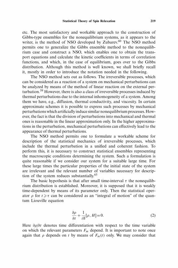
etc. The most satisfactory and workable approach to the construction ofGibbs-type ensembles for the nonequilibrium systems, as it appears to thewriter, is the method of NSO developed by Zubarev.60 The NSO methodpermits one to generalize the Gibbs ensemble method to the nonequilib-rium case and construct a NSO, which enables one to obtain the trans-port equations and calculate the kinetic coefficients in terms of correlationfunctions, and which, in the case of equilibrium, goes over to the Gibbsdistribution. Although this method is well known, we shall briefly recallit, mostly in order to introduce the notation needed in the following.
The NSO method sets out as follows. The irreversible processes, whichcan be considered as a reaction of a system on mechanical perturbations canbe analyzed by means of the method of linear reaction on the external per-turbation.59 However, there is also a class of irreversible processes induced bythermal perturbations due to the internal inhomogeneity of a system. Amongthem we have, e.g., diffusion, thermal conductivity, and viscosity. In certainapproximate schemes it is possible to express such processes by mechanicalperturbations which artificially induce similar nonequilibrium processes. How-ever, the fact is that the division of perturbations into mechanical and thermalones is reasonable in the linear approximation only. In the higher approxima-tions in the perturbation, mechanical perturbations can effectively lead to theappearance of thermal perturbations.
The NSO method permits one to formulate a workable scheme fordescription of the statistical mechanics of irreversible processes, whichinclude the thermal perturbation in a unified and coherent fashion. Toperform this, it is necessary to construct statistical ensembles representingthe macroscopic conditions determining the system. Such a formulation isquite reasonable if we consider our system for a suitable large time. Forthese large times the particular properties of the initial state of the systemare irrelevant and the relevant number of variables necessary for descrip-tion of the system reduces substantially.65
The basic hypothesis is that after small time-interval τ the nonequilib-rium distribution is established. Moreover, it is supposed that it is weaklytime-dependent by means of its parameter only. Then the statistical oper-ator ρ for t�τ can be considered as an “integral of motion” of the quan-tum Liouville equation
∂ρ
∂t+ 1i–h
[ρ,H ]=0. (2)
Here ∂ρ/∂t denotes time differentiation with respect to the time variableon which the relevant parameters Fm depend. It is important to note onceagain that ρ depends on t by means of Fm(t) only. We may consider that
220 A. L. Kuzemsky
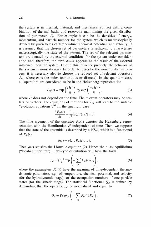
the system is in thermal, material, and mechanical contact with a com-bination of thermal baths and reservoirs maintaining the given distribu-tion of parameters Fm. For example, it can be the densities of energy,momentum, and particle number for the system which is macroscopicallydefined by given fields of temperature, chemical potential, and velocity. Itis assumed that the chosen set of parameters is sufficient to characterizemacroscopically the state of the system. The set of the relevant parame-ters are dictated by the external conditions for the system under consider-ation and, therefore, the term ∂ρ/∂t appears as the result of the externalinfluence upon the system. Due to this influence precisely, the behavior ofthe system is nonstationary. In order to describe the nonequilibrium pro-cess, it is necessary also to choose the reduced set of relevant operatorsPm, where m is the index (continuous or discrete). In the quantum case,all operators are considered to be in the Heisenberg representation
Pm(t)= exp(iH t
–h
)Pm exp
(−iH t–h
), (3)
where H does not depend on the time. The relevant operators may be sca-lars or vectors. The equations of motions for Pm will lead to the suitable“evolution equations”.60 In the quantum case
∂Pm(t)
∂t− 1i–h
[Pm(t),H ]=0. (4)
The time argument of the operator Pm(t) denotes the Heisenberg repre-sentation with the Hamiltonian H independent of time. Then, we supposethat the state of the ensemble is described by a NSO, which is a functionalof Pm(t)
ρ(t)=ρ{. . . Pm(t) . . . }. (5)
Then ρ(t) satisfies the Liouville equation (2). Hence the quasi-equilibrium(“local-equilibrium”) Gibbs-type distribution will have the form
ρq =Q−1q exp
(−∑m
Fm(t)Pm
), (6)
where the parameters Fm(t) have the meaning of time-dependent thermo-dynamic parameters, e.g., of temperature, chemical potential, and velocity(for the hydrodynamic stage), or the occupation numbers of one-particlestates (for the kinetic stage). The statistical functional Qq is defined bydemanding that the operator ρq be normalized and equal to
Qq =T r exp
(−∑m
Fm(t)Pm
). (7)
Statistical Theory of Spin Relaxation 221
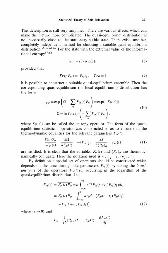
This description is still very simplified. There are various effects, which canmake the picture more complicated. The quasi-equilibrium distribution isnot necessarily close to the stationary stable state. There exists another,completely independent method for choosing a suitable quasi-equilibriumdistribution.56,57,61,67 For the state with the extremal value of the informa-tional entropy57,61
S=−T r(ρ lnρ), (8)
provided that
T r(ρPm)=〈Pm〉q, T rρ=1 (9)
it is possible to construct a suitable quasi-equilibrium ensemble. Then thecorresponding quasi-equilibrium (or local equilibrium ) distribution hasthe form
ρq = exp
(�−
∑m
Fm(t)Pm
)≡ exp(−S(t,0)),
�= lnT r exp
(−∑m
Fm(t)Pm
),
(10)
where S(t,0) can be called the entropy operator. The form of the quasi-equilibrium statistical operator was constructed so as to ensure that thethermodynamic equalities for the relevant parameters Fm(t)
δ lnQq
δFm(t)= δ�
δFm(t)=−〈Pm〉q, δS
δ〈Pm〉q =Fm(t) (11)
are satisfied. It is clear that the variables Fm(t) and 〈Pm〉q are thermody-namically conjugate. Here the notation used is 〈. . . 〉q =T r(ρq . . . ).
By definition a special set of operators should be constructed whichdepends on the time through the parameters Fm(t) by taking the invari-ant part of the operators Fm(t)Pm occurring in the logarithm of thequasi-equilibrium distribution, i.e.,
Bm(t) = Fm(t)Pm= ε∫ 0
−∞eεt1Fm(t+ t1)Pm(t1)dt1
= Fm(t)Pm−∫ 0
−∞dt1e
εt1(Fm(t+ t1)Pm(t1)
+Fm(t+ t1)Pm(t1)), (12)
where (ε→0) and
Pm= 1i–h
[Pm,H ], Fm(t)= dFm(t)
dt.
222 A. L. Kuzemsky
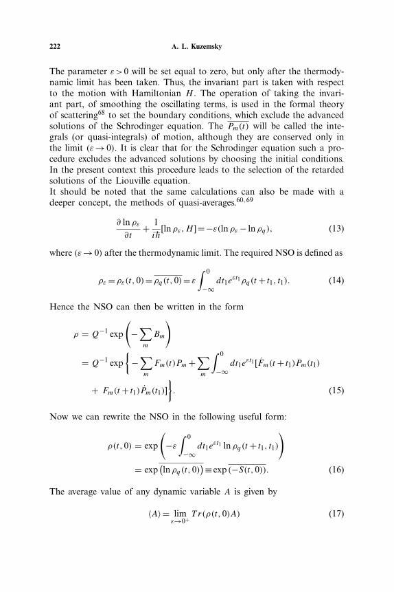
The parameter ε>0 will be set equal to zero, but only after the thermody-namic limit has been taken. Thus, the invariant part is taken with respectto the motion with Hamiltonian H . The operation of taking the invari-ant part, of smoothing the oscillating terms, is used in the formal theoryof scattering68 to set the boundary conditions, which exclude the advancedsolutions of the Schrodinger equation. The Pm(t) will be called the inte-grals (or quasi-integrals) of motion, although they are conserved only inthe limit (ε→0). It is clear that for the Schrodinger equation such a pro-cedure excludes the advanced solutions by choosing the initial conditions.In the present context this procedure leads to the selection of the retardedsolutions of the Liouville equation.It should be noted that the same calculations can also be made with adeeper concept, the methods of quasi-averages.60,69
∂ lnρε∂t
+ 1i–h
[lnρε,H ]=−ε(lnρε− lnρq), (13)
where (ε→0) after the thermodynamic limit. The required NSO is defined as
ρε=ρε(t,0)=ρq(t,0)= ε∫ 0
−∞dt1e
εt1ρq(t+ t1, t1). (14)
Hence the NSO can then be written in the form
ρ = Q−1 exp
(−∑m
Bm
)
= Q−1 exp{
−∑m
Fm(t)Pm+∑m
∫ 0
−∞dt1e
εt1 [Fm(t+ t1)Pm(t1)
+ Fm(t+ t1)Pm(t1)]}. (15)
Now we can rewrite the NSO in the following useful form:
ρ(t,0) = exp
(−ε
∫ 0
−∞dt1e
εt1 lnρq(t+ t1, t1))
= exp(lnρq(t,0)
)≡ exp (−S(t,0)). (16)
The average value of any dynamic variable A is given by
〈A〉= limε→0+
T r(ρ(t,0)A) (17)
Statistical Theory of Spin Relaxation 223
and is, in fact, the quasi-average. The normalization of the quasi-equilib-rium distribution ρq will persists after taking the invariant part if the fol-lowing conditions are required
T r(ρ(t,0)Pm)=〈Pm〉=〈Pm〉q, T rρ=1. (18)
Before closing this section, we shall mention some modification of the“canonical” NSO method which was proposed in Ref. 67 and which onehas to take into account in a more accurate treatment of transport pro-cesses.
2.2. Transport and Kinetic Equations
It is well known that the kinetic equations are of great interest in thetheory of transport processes. Indeed, as it was shown in the precedingsection, the main quantities involved are the following thermodynamicallyconjugate values:
〈Pm〉=− δ�
δFm(t), Fm(t)= δS
δ〈Pm〉 . (19)
The generalized transport equations, which describe the time evolution ofvariables 〈Pm〉 and Fm follow from the equation of motion for the Pm,averaged with the NSO (16). It reads
〈Pm〉=−∑n
δ2�
δFm(t)δFn(t)Fn(t), Fm(t)=
∑n
δ2S
δ〈Pm〉δ〈Pn〉 〈Pn〉. (20)
The entropy production has the form
S(t)=〈S(t,0)〉=−∑m
〈Pm〉Fm(t)=−∑n,m
δ2�
δFm(t)δFn(t)Fn(t)Fm(t). (21)
These equations are the mutually conjugate and with Eq. (19) form acomplete system of equations for the calculation of values 〈Pm〉 and Fm.
2.3. System in Thermal Bath: Generalized Kinetic Equations
In paper,64 we derived the generalized kinetic equations for the sys-tem weakly coupled to a thermal bath. Examples of such systems can bean atomic (or molecular) system interacting with the electromagnetic fieldit generates as with a thermal bath, a system of nuclear or electronic spinsinteracting with the lattice, etc. The aim was to describe the relaxationprocesses in two weakly interacting subsystems, one of which is in the
224 A. L. Kuzemsky
nonequilibrium state and the other is considered as a thermal bath. Theconcept of thermal bath or heat reservoir, i.e., a system that has effectivelyan infinite number of degrees of freedom, was not formulated precisely. Astandard definition of the thermal bath is a heat reservoir defining a tem-perature of the system environment. From a mathematical point of view,66
a heat bath is something that gives a stochastic influence on the systemunder consideration. In this sense, the generalized master equation70 is atool for extracting the dynamics of a subsystem of a larger system by theuse of a special projection techniques71 or special expansion technique.72
The problem of a small system weakly interacting with a heat reservoirhas various aspects. Basic to the derivation of a transport equation for asmall system weakly interacting with a heat bath is a proper introductionof model assumptions. We are interested here in the problem of deriva-tion of the kinetic equations for a certain set of average values (occupa-tion numbers, spins, etc.), which characterize the nonequilibrium state ofthe system.
The Hamiltonian of the total system is taken in the following form:
H =H1 +H2 +V, (22)
where
H1 =∑α
Eαa†αaα, V =
∑α,β
�αβa†αaβ, �αβ =�†
βα. (23)
Here H1 is the Hamiltonian of the small subsystem, and a†α and aα are
the creation and annihilation second quantized operators of quasiparti-cles in the small subsystem with energies Eα, V is the operator of theinteraction between the small subsystem and the thermal bath, and H2 theHamiltonian of the thermal bath which we do not write explicitly. Thequantities �αβ are the operators acting on the thermal bath variables.
We assume that the state of this system is determined completely bythe set of averages 〈Pαβ〉 = 〈a†
αaβ〉 and the state of the thermal bath by〈H2〉, where 〈. . . 〉 denotes the statistical average with the NSO, which willbe defined below.
We take the quasi-equilibrium statistical operator ρq in the form
ρq(t)= exp(−S(t,0)), S(t,0)=�(t)+∑αβ
PαβFαβ(t)+βH2
�= lnT r exp(−∑αβ
PαβFαβ(t)−βH2). (24)
Here Fαβ(t) are the thermodynamic parameters conjugated with Pαβ , andβ is the reciprocal temperature of the thermal bath. All the operators are
Statistical Theory of Spin Relaxation 225
considered in the Heisenberg representation. The NSO has the form
ρ(t)= exp(−S(t,0)), (25)
S(t,0)= ε∫ 0
−∞dt1e
εt1
⎛⎝�(t+ t1)+∑
αβ
PαβFαβ(t)+βH2
⎞⎠ . (26)
The parameters Fαβ(t) are determined from the condition 〈Pαβ〉=〈Pαβ〉q .In the derivation of the kinetic equations we use the perturbation the-
ory in a “weakness of interaction” and assume that the equality 〈�αβ〉q=0holds, while other terms can be added to the renormalized energy of thesubsystem. For further considerations it is convenient to rewrite ρq as
ρq =ρ1ρ2 =Q−1q exp(−L0(t)), (27)
where
ρ1 = Q−11 exp
⎛⎝−
∑αβ
PαβFαβ(t)
⎞⎠ ,
Q1 = T r exp
⎛⎝−
∑αβ
PαβFαβ(t)
⎞⎠ , (28)
ρ2 = Q−12 e−βH2 , Q2 =T r exp(−βH2), (29)
Qq = Q1Q2, L0 =∑αβ
PαβFαβ(t)+βH2. (30)
We now turn to the derivation of the kinetic equations. The starting pointis the kinetic equations in the following implicit form:
d〈Pαβ〉dt
= 1i–h
〈[Pαβ,H ]〉= 1i–h(Eβ −Eα)〈Pαβ〉+ 1
i–h〈[Pαβ,V ]〉. (31)
We restrict ourselves to the second-order in powers of V in calculatingthe r.h.s. of (31). Finally, we obtain the kinetic equations for 〈Pαβ〉 in theform64
d〈Pαβ〉dt
= 1i–h(Eβ −Eα)〈Pαβ〉− 1
–h2
∫ 0
−∞dt1e
εt1⟨[
[Pαβ,V ], V (t1)]⟩q. (32)
The last term of the right-hand side of Eq.(32) can be called the gen-eralized “collision integral”. Thus, we can see that the collision term forthe system weakly coupled to the thermal bath has a convenient form ofthe double commutator as for the generalized kinetic equations73 for thesystem with small interaction. It should be emphasized that the assump-tion about the model form of the Hamiltonian (22) is nonessential for
226 A. L. Kuzemsky
the above derivation. We can start again with the Hamiltonian (22) inwhich we shall not specify the explicit form of H1 and V . We assumethat the state of the nonequilibrium system is characterized completely bysome set of average values 〈Pk〉 and the state of the thermal bath by 〈H2〉.We confine ourselves to such systems for which [H1, Pk] =
∑l cklPl . Then
we assume that 〈V 〉q �0, where 〈. . . 〉q denotes the statistical average withthe quasi-equilibrium statistical operator of the form
ρq =Q−1q exp
(−∑k
PkFk(t)−βH2
)(33)
and Fk(t) are the parameters conjugated with 〈Pk〉. Following the methodused above in the derivation of equation (32), we can obtain the general-ized kinetic equations for 〈Pk〉 with an accuracy up to terms, which arequadratic in interaction
d〈Pk〉dt
= i–h
∑l
ckl〈Pl〉− 1–h2
∫ 0
−∞dt1e
εt1〈[[Pk,V ], V (t1)]〉q . (34)
Hence (32) is fulfilled for the general form of the Hamiltonian of a smallsystem weakly coupled to a thermal bath.
2.4. System in Thermal Bath: Rate and Master Equations
In Sec. 2.3, we have described the kinetic equations for 〈Pαβ〉 in thegeneral form. Let us write down Eq. (32) in an explicit form. We rewritethe kinetic equations for 〈Pαβ〉 as
d〈Pαβ〉dt
= 1i–h(Eβ−Eα)〈Pαβ〉−
∑ν
(Kβν〈Pαν〉+K†
αν〈Pνβ〉)
+∑μν
Kαβ,μν〈Pμν〉.
(35)
The following notation were used
1i–h
∑μ
∫ 0
−∞dt1e
εt1〈�βμφμν(t1)〉q
= 12π
∑μ
∫ +∞
−∞dω
Jμν,βμ(ω)–hω−Eγ −Eδ + iε =Kβν, (36)
1i–h
∫ 0
−∞dt1e
εt1(〈�μαφβν(t1)〉q +〈φμα(t1)�βν〉q)
Statistical Theory of Spin Relaxation 227
= 12π
∫ +∞
−∞dωJβν,μα(ω)
(1
–hω−Eβ +Eν + iε − 1–hω−Eα −Eμ− iε
)
=Kαβ,μν.
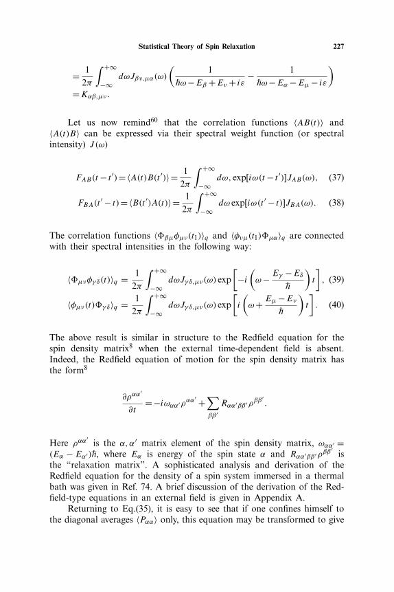
Let us now remind60 that the correlation functions 〈AB(t)〉 and〈A(t)B〉 can be expressed via their spectral weight function (or spectralintensity) J (ω)
FAB(t− t ′)=〈A(t)B(t ′)〉= 12π
∫ +∞
−∞dω, exp[iω(t− t ′)]JAB(ω), (37)
FBA(t′ − t)=〈B(t ′)A(t)〉= 1
2π
∫ +∞
−∞dω exp[iω(t ′ − t)]JBA(ω). (38)
The correlation functions 〈�βμφμν(t1)〉q and 〈φνμ(t1)�μα〉q are connectedwith their spectral intensities in the following way:
〈�μνφγ δ(t)〉q = 12π
∫ +∞
−∞dωJγ δ,μν(ω) exp
[−i(ω− Eγ −Eδ
–h
)t
], (39)
〈φμν(t)�γ δ〉q = 12π
∫ +∞
−∞dωJγ δ,μν(ω) exp
[i
(ω+ Eμ−Eν
–h
)t
]. (40)
The above result is similar in structure to the Redfield equation for thespin density matrix8 when the external time-dependent field is absent.Indeed, the Redfield equation of motion for the spin density matrix hasthe form8
∂ραα′
∂t=−iωαα′ραα
′ +∑ββ ′
Rαα′ββ ′ρββ′.
Here ραα′
is the α,α′ matrix element of the spin density matrix, ωαα′ =(Eα − Eα′)–h, where Eα is energy of the spin state α and Rαα′ββ ′ρββ
′is
the “relaxation matrix”. A sophisticated analysis and derivation of theRedfield equation for the density of a spin system immersed in a thermalbath was given in Ref. 74. A brief discussion of the derivation of the Red-field-type equations in an external field is given in Appendix A.
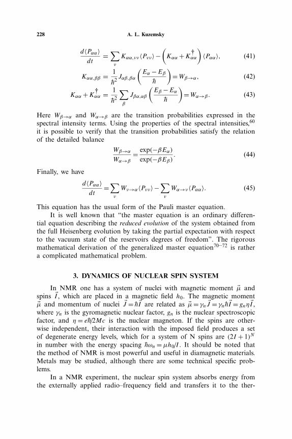
Returning to Eq.(35), it is easy to see that if one confines himself tothe diagonal averages 〈Pαα〉 only, this equation may be transformed to give
228 A. L. Kuzemsky
d〈Pαα〉dt
=∑ν
Kαα,νν〈Pνν〉−(Kαα +K†
αα
)〈Pαα〉, (41)
Kαα,ββ = 1–h2Jαβ,βα
(Eα −Eβ
–h
)=Wβ→α, (42)
Kαα +K†αα = 1
–h2
∑β
Jβα,αβ
(Eβ −Eα
–h
)=Wα→β. (43)
Here Wβ→α and Wα→β are the transition probabilities expressed in thespectral intensity terms. Using the properties of the spectral intensities,60
it is possible to verify that the transition probabilities satisfy the relationof the detailed balance
Wβ→α
Wα→β
= exp(−βEα)exp(−βEβ) . (44)
Finally, we have
d〈Pαα〉dt
=∑ν
Wν→α〈Pνν〉−∑ν
Wα→ν〈Pαα〉. (45)
This equation has the usual form of the Pauli master equation.It is well known that “the master equation is an ordinary differen-
tial equation describing the reduced evolution of the system obtained fromthe full Heisenberg evolution by taking the partial expectation with respectto the vacuum state of the reservoirs degrees of freedom”. The rigorousmathematical derivation of the generalized master equation70–72 is rathera complicated mathematical problem.
3. DYNAMICS OF NUCLEAR SPIN SYSTEM
In NMR one has a system of nuclei with magnetic moment �μ andspins �I , which are placed in a magnetic field h0. The magnetic moment�μ and momentum of nuclei �J = –h �I are related as �μ= γn �J = γn–h �I = gnη �I ,where γn is the gyromagnetic nuclear factor, gn is the nuclear spectroscopicfactor, and η = e–h/2Mc is the nuclear magneton. If the spins are other-wise independent, their interaction with the imposed field produces a setof degenerate energy levels, which for a system of N spins are (2I + 1)N
in number with the energy spacing –hωn =μh0/I . It should be noted thatthe method of NMR is most powerful and useful in diamagnetic materials.Metals may be studied, although there are some technical specific prob-lems.
In a NMR experiment, the nuclear spin system absorbs energy fromthe externally applied radio–frequency field and transfers it to the ther-
Statistical Theory of Spin Relaxation 229
mal bath or reservoir provided by the lattice through the spin-lattice inter-actions. The latter process requires a time interval of the order of thespin-lattice relaxation time T1. The term “lattice” is used here to denotethe equilibrium heat reservoir with temperature T associated with alldegrees of freedom of the system other than those associated with thenuclear spins.
A great advantage of magnetic resonance method is that the nuclearspin system is only very weakly coupled to the other degrees of free-dom of the complex system in which it resides and its thermal capacity isextremely small. It is, therefore, possible to cause the nuclear spin systemitself to depart severely from thermal equilibrium while leaving the rest ofthe material essentially in thermal equilibrium. As a consequence, the dis-turbance of the system other than the nuclear spins could be ignored.
If the nuclei are in thermodynamic equilibrium with the material attemperature T in a field h0, a nuclear paramagnetic moment M0 is pro-duced in the direction of h0 given by the Curie formula M0/h0 =nμ2/3kT ,n is the number of nuclei per unit volume.
We can evidently disturb the system from equilibrium by applyingradiation from outside with quanta of size –hωn and with suitable polar-ization. If the equilibrium distribution is disturbed and the populationchanged, the magnetization in the z-direction, Mz, is different from M0,say Mh
z . If then left alone, Mz reverts to M0 and usually does so exponen-tially with time, i.e.
Mz(t)=M0 − (M0 −Mhz ) exp
{− t
T1
}.
The last expression serves to define the spin–lattice relaxation time, T1,and is so called because the process involves exchange of magnetic orienta-tion energy with thermal energy of other degrees of freedom (known con-ventionally as a lattice). All the interactions with the nucleus may contrib-ute to the relaxation process so we must add all contributions to 1/T1
1T1
∝ 1T1α
+ 1T1β
+ 1T1γ
+ . . . ,
where various contributions to relaxation due to various interactions havebeen added. The relaxation rates may be dominated by one or more differ-ent physical interactions, so that the observable power spectrum may bethe Fourier transform of functions involving dipole–dipole correlations,electric field gradient-nuclear quadrupole moment correlations, etc.
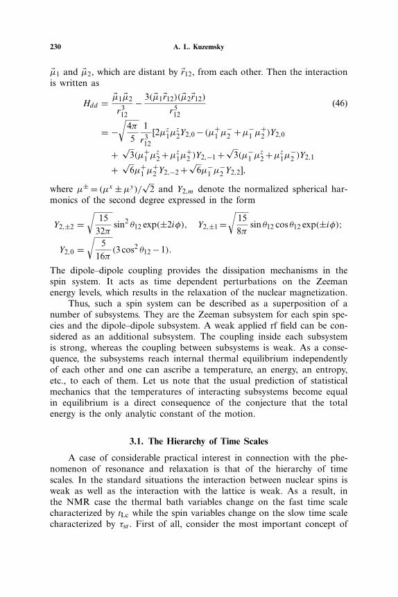
The dipole–dipole interaction Hamiltonian Hdd between the magneticmoments of nuclei may contribute significantly to the nuclear magneticrelaxation process.75 Consider an explicit interaction between the moments
230 A. L. Kuzemsky
�μ1 and �μ2, which are distant by �r12, from each other. Then the interactionis written as
Hdd = �μ1 �μ2
r312
− 3( �μ1�r12)( �μ2�r12)
r512
(46)
= −√
4π5
1
r312
[2μz1μz2Y2,0 − (μ+
1 μ−2 +μ−
1 μ+2 )Y2,0
+√
3(μ+1 μ
z2 +μz1μ+
2 )Y2,−1 +√
3(μ−1 μ
z2 +μz1μ−
2 )Y2,1
+√
6μ+1 μ
+2 Y2,−2 +
√6μ−
1 μ−2 Y2,2],
where μ± = (μx ±μy)/√2 and Y2,m denote the normalized spherical har-monics of the second degree expressed in the form
Y2,±2 =√
1532π
sin2 θ12 exp(±2iφ), Y2,±1 =√
158π
sin θ12 cos θ12 exp(±iφ);
Y2,0 =√
516π
(3 cos2 θ12 −1).
The dipole–dipole coupling provides the dissipation mechanisms in thespin system. It acts as time dependent perturbations on the Zeemanenergy levels, which results in the relaxation of the nuclear magnetization.
Thus, such a spin system can be described as a superposition of anumber of subsystems. They are the Zeeman subsystem for each spin spe-cies and the dipole–dipole subsystem. A weak applied rf field can be con-sidered as an additional subsystem. The coupling inside each subsystemis strong, whereas the coupling between subsystems is weak. As a conse-quence, the subsystems reach internal thermal equilibrium independentlyof each other and one can ascribe a temperature, an energy, an entropy,etc., to each of them. Let us note that the usual prediction of statisticalmechanics that the temperatures of interacting subsystems become equalin equilibrium is a direct consequence of the conjecture that the totalenergy is the only analytic constant of the motion.
3.1. The Hierarchy of Time Scales
A case of considerable practical interest in connection with the phe-nomenon of resonance and relaxation is that of the hierarchy of timescales. In the standard situations the interaction between nuclear spins isweak as well as the interaction with the lattice is weak. As a result, inthe NMR case the thermal bath variables change on the fast time scalecharacterized by tLc while the spin variables change on the slow time scalecharacterized by τsr. First of all, consider the most important concept of
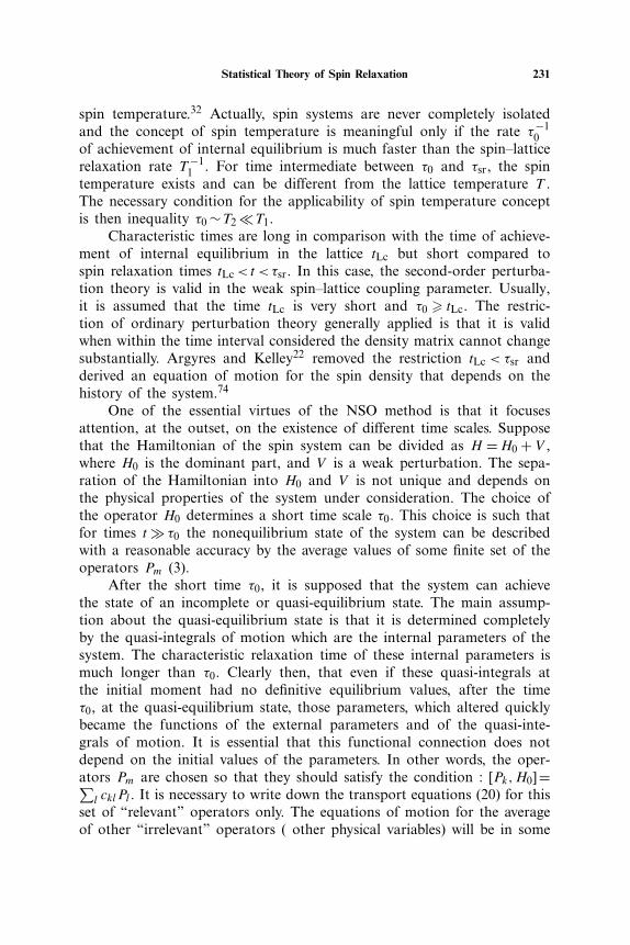
Statistical Theory of Spin Relaxation 231
spin temperature.32 Actually, spin systems are never completely isolatedand the concept of spin temperature is meaningful only if the rate τ−1
0of achievement of internal equilibrium is much faster than the spin–latticerelaxation rate T −1
1 . For time intermediate between τ0 and τsr, the spintemperature exists and can be different from the lattice temperature T .The necessary condition for the applicability of spin temperature conceptis then inequality τ0 ∼T2 �T1.
Characteristic times are long in comparison with the time of achieve-ment of internal equilibrium in the lattice tLc but short compared tospin relaxation times tLc<t <τsr. In this case, the second-order perturba-tion theory is valid in the weak spin–lattice coupling parameter. Usually,it is assumed that the time tLc is very short and τ0 � tLc. The restric-tion of ordinary perturbation theory generally applied is that it is validwhen within the time interval considered the density matrix cannot changesubstantially. Argyres and Kelley22 removed the restriction tLc < τsr andderived an equation of motion for the spin density that depends on thehistory of the system.74
One of the essential virtues of the NSO method is that it focusesattention, at the outset, on the existence of different time scales. Supposethat the Hamiltonian of the spin system can be divided as H =H0 + V ,where H0 is the dominant part, and V is a weak perturbation. The sepa-ration of the Hamiltonian into H0 and V is not unique and depends onthe physical properties of the system under consideration. The choice ofthe operator H0 determines a short time scale τ0. This choice is such thatfor times t � τ0 the nonequilibrium state of the system can be describedwith a reasonable accuracy by the average values of some finite set of theoperators Pm (3).
After the short time τ0, it is supposed that the system can achievethe state of an incomplete or quasi-equilibrium state. The main assump-tion about the quasi-equilibrium state is that it is determined completelyby the quasi-integrals of motion which are the internal parameters of thesystem. The characteristic relaxation time of these internal parameters ismuch longer than τ0. Clearly then, that even if these quasi-integrals atthe initial moment had no definitive equilibrium values, after the timeτ0, at the quasi-equilibrium state, those parameters, which altered quicklybecame the functions of the external parameters and of the quasi-inte-grals of motion. It is essential that this functional connection does notdepend on the initial values of the parameters. In other words, the oper-ators Pm are chosen so that they should satisfy the condition : [Pk,H0]=∑l cklPl . It is necessary to write down the transport equations (20) for this
set of “relevant” operators only. The equations of motion for the averageof other “irrelevant” operators ( other physical variables) will be in some
232 A. L. Kuzemsky
sense consequences of these transport equations. As for the “irrelevant”operators, which do not belong to the reduced set of the “relevant” opera-tors Pm, relation [Pk,H0]=∑l cklPl leads to the infinite chain of operatorequalities. For times t� τ0 the nonequilibrium averages of these operatorsoscillate fast, while for times t > τ0 they become functions of the averagevalues of the operators.
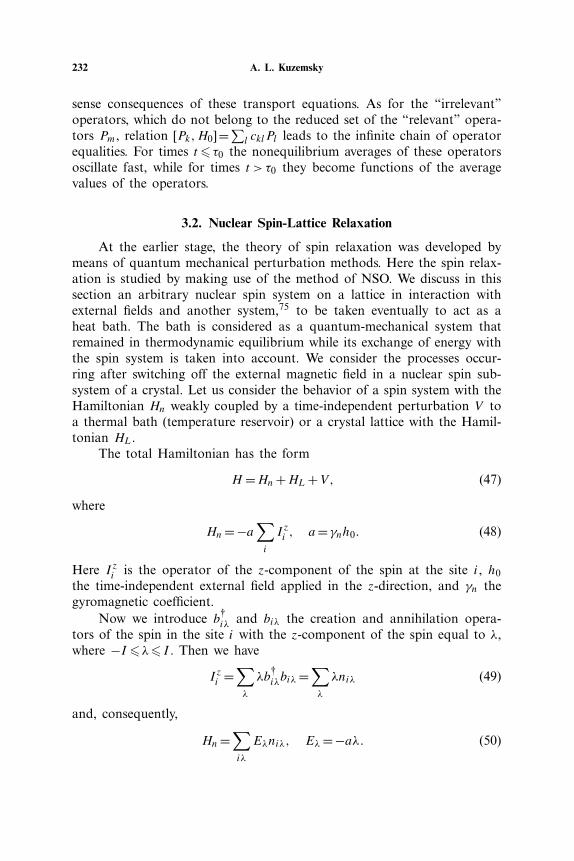
3.2. Nuclear Spin-Lattice Relaxation
At the earlier stage, the theory of spin relaxation was developed bymeans of quantum mechanical perturbation methods. Here the spin relax-ation is studied by making use of the method of NSO. We discuss in thissection an arbitrary nuclear spin system on a lattice in interaction withexternal fields and another system,75 to be taken eventually to act as aheat bath. The bath is considered as a quantum-mechanical system thatremained in thermodynamic equilibrium while its exchange of energy withthe spin system is taken into account. We consider the processes occur-ring after switching off the external magnetic field in a nuclear spin sub-system of a crystal. Let us consider the behavior of a spin system with theHamiltonian Hn weakly coupled by a time-independent perturbation V toa thermal bath (temperature reservoir) or a crystal lattice with the Hamil-tonian HL.
The total Hamiltonian has the form
H =Hn+HL+V, (47)
where
Hn=−a∑i
I zi , a=γnh0. (48)
Here I zi is the operator of the z-component of the spin at the site i, h0the time-independent external field applied in the z-direction, and γn thegyromagnetic coefficient.
Now we introduce b†iλ and biλ the creation and annihilation opera-
tors of the spin in the site i with the z-component of the spin equal to λ,where −I �λ� I . Then we have
I zi =∑λ
λb†iλbiλ=
∑λ
λniλ (49)
and, consequently,
Hn=∑iλ
Eλniλ, Eλ=−aλ. (50)
Statistical Theory of Spin Relaxation 233
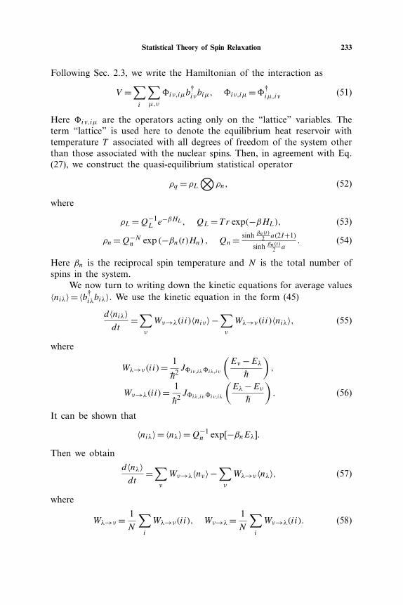
Following Sec. 2.3, we write the Hamiltonian of the interaction as
V =∑i
∑μ,ν
�iν,iμb†iνbiμ, �iν,iμ=�†
iμ,iν (51)
Here �iν,iμ are the operators acting only on the “lattice” variables. Theterm “lattice” is used here to denote the equilibrium heat reservoir withtemperature T associated with all degrees of freedom of the system otherthan those associated with the nuclear spins. Then, in agreement with Eq.(27), we construct the quasi-equilibrium statistical operator
ρq =ρL⊗
ρn, (52)
where
ρL=Q−1L e−βHL, QL=T r exp(−βHL), (53)
ρn=Q−Nn exp (−βn(t)Hn) , Qn= sinh βn(t)
2 a(2I+1)
sinh βn(t)2 a
. (54)
Here βn is the reciprocal spin temperature and N is the total number ofspins in the system.
We now turn to writing down the kinetic equations for average values〈niλ〉=〈b†
iλbiλ〉. We use the kinetic equation in the form (45)
d〈niλ〉dt
=∑ν
Wν→λ(ii)〈niν〉−∑ν
Wλ→ν(ii)〈niλ〉, (55)
where
Wλ→ν(ii)= 1–h2J�iν,iλ�iλ,iν
(Eν −Eλ
–h
),
Wν→λ(ii)= 1–h2J�iλ,iν�iν,iλ
(Eλ−Eν
–h
). (56)
It can be shown that
〈niλ〉=〈nλ〉=Q−1n exp[−βnEλ].
Then we obtain
d〈nλ〉dt
=∑ν
Wν→λ〈nν〉−∑ν
Wλ→ν〈nλ〉, (57)
where
Wλ→ν = 1N
∑i
Wλ→ν(ii), Wν→λ= 1N
∑i
Wν→λ(ii). (58)
234 A. L. Kuzemsky
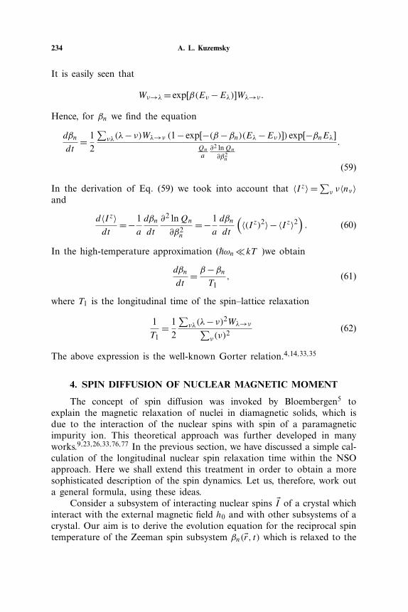
It is easily seen that
Wν→λ= exp[β(Eν −Eλ)]Wλ→ν .
Hence, for βn we find the equation
dβn
dt= 1
2
∑νλ(λ−ν)Wλ→ν (1− exp[−(β−βn)(Eλ−Eν)]) exp[−βnEλ]
Qna∂2 lnQn∂β2n
.
(59)
In the derivation of Eq. (59) we took into account that 〈I z〉 =∑ν ν〈nν〉
and
d〈I z〉dt
=−1a
dβn
dt
∂2 lnQn
∂β2n
=−1a
dβn
dt
(〈(I z)2〉−〈I z〉2
). (60)
In the high-temperature approximation (–hωn�kT )we obtain
dβn
dt= β−βn
T1, (61)
where T1 is the longitudinal time of the spin–lattice relaxation
1T1
= 12
∑νλ(λ−ν)2Wλ→ν∑
ν(ν)2
(62)
The above expression is the well-known Gorter relation.4,14,33,35
4. SPIN DIFFUSION OF NUCLEAR MAGNETIC MOMENT
The concept of spin diffusion was invoked by Bloembergen5 toexplain the magnetic relaxation of nuclei in diamagnetic solids, which isdue to the interaction of the nuclear spins with spin of a paramagneticimpurity ion. This theoretical approach was further developed in manyworks.9,23,26,33,76,77 In the previous section, we have discussed a simple cal-culation of the longitudinal nuclear spin relaxation time within the NSOapproach. Here we shall extend this treatment in order to obtain a moresophisticated description of the spin dynamics. Let us, therefore, work outa general formula, using these ideas.
Consider a subsystem of interacting nuclear spins �I of a crystal whichinteract with the external magnetic field h0 and with other subsystems of acrystal. Our aim is to derive the evolution equation for the reciprocal spintemperature of the Zeeman spin subsystem βn(�r, t) which is relaxed to the
Statistical Theory of Spin Relaxation 235
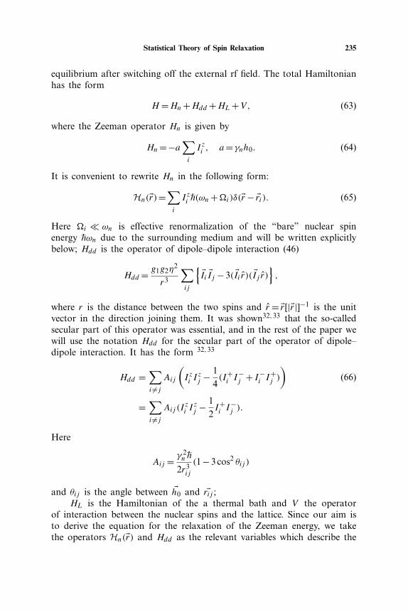
equilibrium after switching off the external rf field. The total Hamiltonianhas the form
H =Hn+Hdd +HL+V, (63)
where the Zeeman operator Hn is given by
Hn=−a∑i
I zi , a=γnh0. (64)
It is convenient to rewrite Hn in the following form:
Hn(�r)=∑i
I zi–h(ωn+�i)δ(�r− �ri). (65)
Here �i � ωn is effective renormalization of the “bare” nuclear spinenergy –hωn due to the surrounding medium and will be written explicitlybelow; Hdd is the operator of dipole–dipole interaction (46)
Hdd = g1g2η2
r3
∑ij
{�Ii �Ij −3( �Ii r)( �Ij r)
},
where r is the distance between the two spins and r = �r[|�r|]−1 is the unitvector in the direction joining them. It was shown32,33 that the so-calledsecular part of this operator was essential, and in the rest of the paper wewill use the notation Hdd for the secular part of the operator of dipole–dipole interaction. It has the form 32,33
Hdd =∑i �=j
Aij
(I zi I
zj − 1
4(I+i I
−j + I−
i I+j )
)(66)
=∑i �=j
Aij (Izi Izj − 1
2I+i I
−j ).
Here
Aij = γ 2n
–h
2r3ij
(1−3 cos2 θij )
and θij is the angle between �h0 and �rij ;HL is the Hamiltonian of the a thermal bath and V the operator
of interaction between the nuclear spins and the lattice. Since our aim isto derive the equation for the relaxation of the Zeeman energy, we takethe operators Hn(�r) and Hdd as the relevant variables which describe the
236 A. L. Kuzemsky
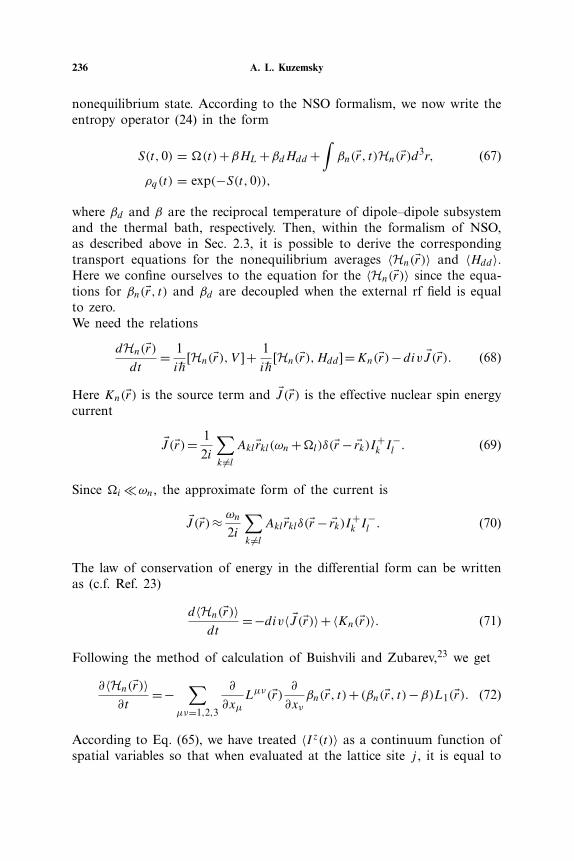
nonequilibrium state. According to the NSO formalism, we now write theentropy operator (24) in the form
S(t,0) = �(t)+βHL+βdHdd +∫βn(�r, t)Hn(�r)d3r, (67)
ρq(t) = exp(−S(t,0)),
where βd and β are the reciprocal temperature of dipole–dipole subsystemand the thermal bath, respectively. Then, within the formalism of NSO,as described above in Sec. 2.3, it is possible to derive the correspondingtransport equations for the nonequilibrium averages 〈Hn(�r)〉 and 〈Hdd〉.Here we confine ourselves to the equation for the 〈Hn(�r)〉 since the equa-tions for βn(�r, t) and βd are decoupled when the external rf field is equalto zero.We need the relations
dHn(�r)dt
= 1i–h
[Hn(�r),V ]+ 1i–h
[Hn(�r),Hdd ]=Kn(�r)−div �J (�r). (68)
Here Kn(�r) is the source term and �J (�r) is the effective nuclear spin energycurrent
�J (�r)= 12i
∑k �=l
Akl�rkl(ωn+�l)δ(�r− �rk)I+k I
−l . (69)
Since �i �ωn, the approximate form of the current is
�J (�r)≈ ωn
2i
∑k �=l
Akl�rklδ(�r− �rk)I+k I
−l . (70)
The law of conservation of energy in the differential form can be writtenas (c.f. Ref. 23)
d〈Hn(�r)〉dt
=−div〈 �J (�r)〉+〈Kn(�r)〉. (71)
Following the method of calculation of Buishvili and Zubarev,23 we get
∂〈Hn(�r)〉∂t
=−∑
μν=1,2,3
∂
∂xμLμν(�r) ∂
∂xνβn(�r, t)+ (βn(�r, t)−β)L1(�r). (72)
According to Eq. (65), we have treated 〈I z(t)〉 as a continuum function ofspatial variables so that when evaluated at the lattice site j , it is equal to
Statistical Theory of Spin Relaxation 237
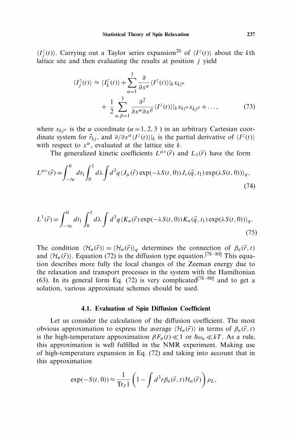
〈I zj (t)〉. Carrying out a Taylor series expansion20 of 〈I z(t)〉 about the kthlattice site and then evaluating the results at position j yield
〈I zj (t)〉 ≈ 〈I zk (t)〉+3∑α=1
∂
∂xα〈I z(t)〉|kxkjα
+ 12
3∑α,β=1
∂2
∂xα∂xβ〈I z(t)〉|kxkjαxkjβ + . . . , (73)
where xkjα is the α coordinate (α=1,2,3 ) in an arbitrary Cartesian coor-dinate system for �rkj , and ∂/∂xα〈I z(t)〉|k is the partial derivative of 〈I z(t)〉with respect to xα, evaluated at the lattice site k.
The generalized kinetic coefficients Lμν(�r) and L1(�r) have the form
Lμν(�r)=∫ 0
−∞dt1
∫ 1
0dλ
∫d3q〈Jμ(�r) exp(−λS(t,0))Jν(�q, t1) exp(λS(t,0))〉q,
(74)
L1(�r)=∫ 0
−∞dt1
∫ 1
0dλ
∫d3q〈Kn(�r) exp(−λS(t,0))Kn(�q, t1) exp(λS(t,0))〉q .
(75)
The condition 〈Hn(�r)〉 = 〈Hn(�r)〉q determines the connection of βn(�r, t)and 〈Hn(�r)〉. Equation (72) is the diffusion type equation.[78–80] This equa-tion describes more fully the local changes of the Zeeman energy due tothe relaxation and transport processes in the system with the Hamiltonian(63). In its general form Eq. (72) is very complicated[78–80] and to get asolution, various approximate schemes should be used.
4.1. Evaluation of Spin Diffusion Coefficient
Let us consider the calculation of the diffusion coefficient. The mostobvious approximation to express the average 〈Hn(�r)〉 in terms of βn(�r, t)is the high-temperature approximation βFn(t)�1 or –hωn�kT . As a rule,this approximation is well fulfilled in the NMR experiment. Making useof high-temperature expansion in Eq. (72) and taking into account that inthis approximation
exp(−S(t,0))≈ 1TrI1
(1−
∫d3rβn(�r, t)Hn(�r)
)ρL,
238 A. L. Kuzemsky
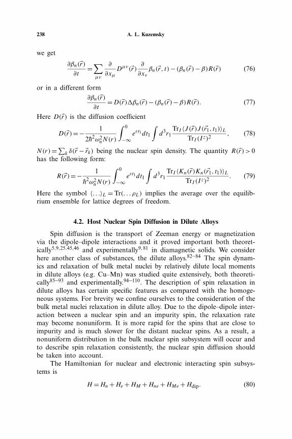
we get
∂βn(�r)∂t
=∑μν
∂
∂xμDμν(�r) ∂
∂xνβn(�r, t)− (βn(�r)−β)R(�r) (76)
or in a different form∂βn(�r)∂t
=D(�r)�βn(�r)− (βn(�r)−β)R(�r). (77)
Here D(�r) is the diffusion coefficient
D(�r)=− 1
2–h2ω2nN(r)
∫ 0
−∞eεt1dt1
∫d3r1
TrI 〈J (�r)J ( �r1, t1)〉LTrI (I z)2
, (78)
N(r)=∑k δ(�r − �rk) being the nuclear spin density. The quantity R(�r)> 0has the following form:
R(�r)=− 1–h2ω2
nN(r)
∫ 0
−∞eεt1dt1
∫d3r1
TrI 〈Kn(�r)Kn( �r1, t1)〉LTrI (I z)2
. (79)
Here the symbol 〈. . .〉L = Tr(. . . ρL) implies the average over the equilib-rium ensemble for lattice degrees of freedom.
4.2. Host Nuclear Spin Diffusion in Dilute Alloys
Spin diffusion is the transport of Zeeman energy or magnetizationvia the dipole–dipole interactions and it proved important both theoret-ically5,9,25,45,46 and experimentally9,81 in diamagnetic solids. We considerhere another class of substances, the dilute alloys.82–84 The spin dynam-ics and relaxation of bulk metal nuclei by relatively dilute local momentsin dilute alloys (e.g. Cu–Mn) was studied quite extensively, both theoreti-cally85–93 and experimentally.94–110. The description of spin relaxation indilute alloys has certain specific features as compared with the homoge-neous systems. For brevity we confine ourselves to the consideration of thebulk metal nuclei relaxation in dilute alloy. Due to the dipole–dipole inter-action between a nuclear spin and an impurity spin, the relaxation ratemay become nonuniform. It is more rapid for the spins that are close toimpurity and is much slower for the distant nuclear spins. As a result, anonuniform distribution in the bulk nuclear spin subsystem will occur andto describe spin relaxation consistently, the nuclear spin diffusion shouldbe taken into account.
The Hamiltonian for nuclear and electronic interacting spin subsys-tems is
H =Hn+He+HM +Hne+HMe+Hdip. (80)
Statistical Theory of Spin Relaxation 239
Here index n denotes the host nuclear spins, M denotes spin of the mag-netic impurities, and e denotes the electron subsystem. In this section,when we refer to the host nuclear spin subsystem Hn we put
Hn=∑i
I zi–hωn+
∑i �=j
Aij (Izi Izj − 1
2I+i I
−j ). (81)
The Hamiltonian of electron subsystem is
He=∑kσ
εkσ a†kσ akσ (82)
and
HM =∑m
–hωMSzm (83)
is the Hamiltonian of the impurity spins in the external magnetic field.The Hamiltonian of the interaction110 of nuclear spins and the spin den-sity �σ( �Ri) of the conduction electrons is
Hne=Jne∑i
�Ii �σ( �Ri), Jne=− 8π–h2γnγe
, (84)
where
σ+k =
∑q
a†q↑ak+q↓, σ−
−k = (σ+k )
† =∑q
a†k+q↓aq↑.
Interaction of the impurity spins �Sm and the spin density of the itinerantcarriers is given by the spin-fermion111,112 (sp−d(f ))model Hamiltonian
HMe=Jsd∑m
�Sm �σ( �Rm). (85)
The last part of the total Hamiltonian (80)
Hdip=–h∑im
∑μν=x,y,z
�μνimI
μi S
νm (86)
is the Hamiltonian of the dipole-dipole and pseudo–dipolar interactionof nuclear and impurity spins. This interaction was described in detail inRefs. 94,95,113. The pseudo–dipolar interaction does not originate in crys-talline anisotropy but in the tensor character of the dipolar interaction.95
Their expression for the pseudo-dipolar interaction is
HPDnn =
∑ij
[�Ii �Ij −3r−2
ij (�Ii �rij )( �Ij �rij )
]Bij . (87)

240 A. L. Kuzemsky
The Van Vleck Hamiltonian for a system with two magnetic ingredi-ents95,113 includes the term
Hdip =∑i>j
(g2nη
2
r3ij
+ Bij){
�Ii �Ij −3r−2ij (
�Ii �rij )( �Ij �rij )}
+∑im
(gngeη
2
r3im
+ Bim){
�Ii �Sm−3r−2ij (
�Ii �rim)(�Sm �rim)}
+∑m>n
(g2e η
2
r3mn
+ Bmn){
�Sm �Sn−3r−2mn(
�Si �rmn)(�Sj �rmn)}. (88)
The B’s represent the pseudo-dipolar interaction
Bij = 32
(Bij + g2
nη2
r3ij
)(1−3 cos2 θij ).
The later consists of three components of which we use in Eq.(86) the fol-lowing one as the most essential113,95
HPDMn =
∑im
Bim �Ii(�Sm− rim(rim �Sm)). (89)
It was shown in Ref. 95 that for the large distance between the nuclearspin and the electron spin Bim has the form
Bim≈B cos(kF rim+φB)(2kF rim)3
. (90)
Thus, in structure, the coefficient Bim is similar to the production of thecontact potential and the spatial part of the RKKY interaction.114 As arule, the pseudo-dipolar interaction is less than the contact interaction.The estimations give B∼ 1/3Jne for 205T l. It will be even more valid forcopper since its mass is much less than for T l.
Now the expression for the Hamiltonian Hdip can be rewritten as
Hdip = γnγM–h∑im
1
r3im
{I zi δS
zm(1−3 cos2 θim) (91)
−32
sin θim cos θim[exp(−iφim)I+i δS
zm+ exp(iφim)I
−i δS
zm]}
{1+B cos(2kF rim+φB)
8k3F
}.
Statistical Theory of Spin Relaxation 241
Here we have introduced the mean field 〈Szm〉 and the fluctuating part ofthe impurity spin, namely δSzm=Szm−〈Szm〉. By substituting this definitionof Szm into (84) rewritten in terms of the variable δSzm we obtain
Hne = − 8π–h2γnγe
∑ip
( �Ii �σp)δ( �Ri − �rp) (92)
= Jne∑ip
[(I+i σ
−p + I−
i σ+p )δ(
�Ri − �rp)
+(σ zpδ( �Ri − �rp)−〈σzpδ( �Ri − �rp)〉)I zi],
where ∑p
�σ(�rp)δ( �Ri − �rp)=∑kk′
∑ss′
〈s|�σ |s′〉ψ∗k′(0)ψk(0)a
†ksak′s′ .
Now it is possible to write down explicitly the shift of the Zeeman fre-quency ωn in (65) due to the mean-field renormalization �i as
�i = γnγM–h∑m
1
r3im
{1+B cos(2kF rim+φB)
8k3F
}〈Sz〉
Jne∑p
〈σzpδ( �Ri − �rp)〉=∑m
�zzim〈Szm〉−Jne∑p
〈σzpδ( �Ri − �rp)〉. (93)
This shift of the Zeeman frequency (�i �ωn) is the most essential for theevaluation of the coefficient of spin diffusion.33,37,76
4.3. Spin Diffusion Coefficient in Dilute Alloys
Here, we evaluate concrete expressions for the spin diffusion coefficient(78) for the dilute alloys system which is described by the Hamiltonian(80). Consider again the approximate equation (76) where the diffusioncoefficient can be written as
Dμν ≈ ωd–h2√π
∑l
A2rl(r
μ− rμl )(rν − rνl ) exp[−(�r −�l)2/4 (ωd)2]. (94)
In the derivation of the above expression, to permit explicit calculations,the Gaussian approximation for the nuclear spin correlation function wasused (see Appendix B). From Eqs. (76) and (94) it follows that in the pro-cess of the longitudinal nuclear spin relaxation, which is a function ofposition, there is a possibility to transport the nuclear magnetization (i.e.excess of nuclear spin density) due to the dipole–dipole interaction. It isclearly seen that the nuclei themselves do not move in the spin diffusion
242 A. L. Kuzemsky
process. There is diffusion of the excess of the projection of the nuclearspin only.
To proceed further, consider the case when the concentration of theimpurity spins is very low. In this case, for one impurity spin there is a bignumber of host nuclear spins which interact with it. In other words, thiscase corresponds to the effective single-impurity situation. Thus, we canplace one impurity spin to the origin of the coordinate frame (0,0,0). Thevector �r in Eq. (94) is then counted from this position. For a simple cubiccrystalline system with the inversion center the symmetric tensor Dμν(�r) isreduced to the scalar D(�r). The coefficient D(�r) decreases with decreasingthe distance r when r is small. This is related with the fact that Zeemannuclear frequencies of the nuclei, which are close to the impurity, havesubstantially different values due to the influence of the local magneticfields induced by the impurity spin. This circumstance hinders the flip–flop(�=ωM −ωn) transitions of neighboring nuclei since this transition doesnot conserve the total Zeeman energy of nuclear spins. (Let us remind thatif we suppose that the spins S are completely polarized and the nuclearspins I are completely unpolarized, then the dipolar interaction permitssimultaneous reversals of S and I in the opposite directions, or flip–flops,and also reversals in the same direction which is usually called flip–flipswith �= ωM + ωn). In expression (94) this tendency is described by theexponential factor. This exponential factor leads to the appearance of theso-called “diffusion barrier” around each impurity. Inside this diffusionbarrier the diffusion of nuclear spin is hindered strongly.33,76
It can be seen that for the large distance from the impurity the fre-quency difference in Eq. (94) behaves as (�r − �l) � ωd , where ωd ≈6γ 2n
–ha−3 is the dipolar line-width and D(r) does not depend on r. In theopposite case, of small distance scale (near impurity) the frequency differ-ence is big and the coefficient D(r) decreases quickly with the distance tothe impurity. Thus, it is convenient to introduce the effective radius of thediffusion barrier δ, namely, a distance from the impurity for which the fol-lowing definition holds:
D(r)={D, if r >δ,0, if r <δ.
(95)
The constant D is equal to D=ωd/3–h2√π∑A2klr
2kl .
Let us estimate the “size” of the diffusion barrier. Consider twoneighboring nuclei which take up a position along the radius from theimpurity. The distance between them is equal to the lattice constant a.In this case, the frequency shift is equal to (�δ − �δ+a) ≈ ωd and δ ≈a 4√
[γM/γn〈Sz〉] ( see Appendix B).
Statistical Theory of Spin Relaxation 243
Consider again the approximate Eq.(77) taking into account the diffu-sion barrier approximation (95). It can be rewritten in the form
∂βn(�r, t)∂t
=D�βn(�r, t)− (βn(�r, t)−β)(R0 +R1(�r)+R2(�r)), (96)
where
R0 = 2J 2ne
–h22π
∑kk′
∑pp′
ψ∗k ψk′ψ
∗pψp′
∫ ∞
−∞dωf (ω−ωn)G0
kk′pp′(ω),(97)
G0kk′pp′(ω) =
∫ ∞
−∞dt exp(itω)〈a†
k↓ak′↑a†p↑(t)ap′↓(t)〉, (98)
R1(�r) = −4Jne–h2π
∑kk′
∑m
∫ ∞
−∞dωf (ω−ωn)Re(ψ∗
k ψk′G1kk′m(ω)�
+zrm),(99)
G1kk′m(ω) =
∫ ∞
−∞dt exp(itω)〈a†
k↑ak′↓Szm(t)〉 (100)
and
R2(�r) = 92(γnγM–h)2
12π
∑m
∫ ∞
−∞dωf (ω−ωn)Gimm(ω)Ym, (101)
Gimm(ω) =∫ ∞
−∞dt exp(itω)〈δSzmδSzm(t)〉, (102)
Ym ={
1+ B cos(2kF |�r− �rm|+φB)8k3F
}2sin2 θrm cos2 θrm
|�r− �rm|6 . (103)
Here the function f (ω−ωn) is the NMR line-shape. The line-shape of theNMR spectrum115 arises from the variation of the local field at a givennucleus because of the interaction with nearby neighbors. The inhomoge-neity of the applied magnetic field may also increase the width of the line.
The contribution of the factor R−10 leads to the generalized Korringa
relaxation rate116
1T1
∝ πkT–h
[8π3γn
–hχpM
μe〈|ψF (0)|2〉
]2
. (104)
Korringa116 calculated the spin–lattice relaxation time T1 in metals andshowed that T1 should be inversely proportional to temperature andshould be related to the Knight shift (see also Ref. 117). Korringa nuclear
244 A. L. Kuzemsky
spin-lattice relaxation occurs in a metal through the nucleus-electron inter-action of contact type 116
8π3(|γe|–h�s)(γn–h �I )|ψA(0)|2. (105)
The quantity R1 is determined by the correlation of the electron andimpurity spins and is highly anisotropic.
The quantity R2 is related to the scattering of nuclear spins on thefluctuations of impurity spins. The last contribution is the most essentialfactor in the present context. This is related to the fact that the maincharacteristic features of the problem under consideration clearly manifestitself in the isotropic case which is considered in the majority of works. Inthe isotropic case R1 =0 and the contribution of R2 can be expressed as
R2(r)=∑m
C
{1+ B cos(2kF |�r− �rm|+φB)
8k3F
}21
|�r− �rm|6 , (106)
C= 35(γnγM–h)2
12π
∫ ∞
−∞dωf (ω−ωn)Gimm(ω). (107)
Nevertheless, even after simplifications described above, a solution of thediffusion equation is still a complicated problem. The main difficulty isthe presence of the highly oscillating factor cos(2kF |�r−�rm|+φB). The roleof this oscillating factor can be taken into account entirely by numericalcalculations. For a qualitative rough estimation we consider the simplifiedcase when B ≈ 0. Then we can proceed following the method of calcula-tion of Ref. 76. According to these calculations76 we find
1T1
= (R0)−1 +4πDNF. (108)
Here N is the number of impurities and the quantity F has the form
F ={
0.7b, if b>δ,1/3(b/δ)3b, if b<δ,
(109)
where b= 4√(C/D).
It is clear from Eqs. (108) and (109) that the behavior of the relaxationtime and its value depend strongly on the interrelation of b which is deter-mined by the correlation function Gimm(ω) and of δ which is determinedby 〈Sz〉, as well as on the temperature for each concrete alloy. Thus, theproblem of description of spin–lattice relaxation in dilute metallic alloyswas reduced to the problem of calculation of the value of F . When δ�b
the diffusion barrier is nonessential. In the opposite case, when b<δ, the
Statistical Theory of Spin Relaxation 245
diffusion barrier is essential and leads to the slowing down of the relax-ation process. In other words, the distance b determines the scale up towhich the nuclear spin relaxation is effective. Finally, let us note that theorder of value of time which is necessary to transmit the magnetic momentto the distance r in a solid is equal to τD � r2/D; for r=10−6 cm it givesthe value τD �1 sec.
5. CONCLUDING REMARKS
In the present paper, we have given a complementary method forobtaining the rate and relaxation equations of nuclear spin system in sol-ids. The main tool in this approach is the use of the method of NSO.[60]
We have presented a theory of spin relaxation which allows us to derivegeneral equations of spin dynamics. In addition, our theory allows us totake into account the effects of spin diffusion in a very straightforwardmanner. The calculations were kept general by restricting the form of spin-lattice Hamiltonian as little as possible. It has permitted us to perform thederivation under more general conditions and explicitly demonstrate somekey features of irreversible processes in solids.
It was shown that the spin systems provide a useful proving groundfor applying the sophisticated methods of statistical thermodynamics. Themethod used is capable of systematic improvement and gives a deeperinsight into the meaning of the spin relaxation processes in solids. We haveshown that the transport of nuclear spin energy in a lattice of paramag-netic spins with magnetic dipolar interaction plays an important role inrelaxation processes in solids. To test the general formalism presented here,an example of a dilute metallic alloy system was considered to demon-strate the usefulness of the equations derived.
In summary, the present paper examines the relaxation dynamics of aspin system. It continues the investigation presented in the previous workinto the use of statistical mechanical methods for systems that are in con-tact with a thermal bath. We used the method of the NSO developedby Zubarev. In the present paper, we have developed the application ofthis method to the spin-relaxation problem, so that some useful resultsmay be obtained from it. The calculation presented in this paper can besaid to show that the NSO method has provided a compact and efficienttool for description of the spin relaxation dynamics. In this respect, thepresent treatment may be regarded as a complement of the Buishvili andZubarev23 seminal treatment.
Though the analysis of this paper concentrates on the nuclear spinsystems in solids, the extension to other spin systems, e.g., paramagneticelectron spin system, is straightforward. The other important task is to
246 A. L. Kuzemsky
examine the effects of a periodically time-dependent field on the long-time behavior of an otherwise isolated system of many coupled spins. Thisquestion is a part of a more general problem of the evolution of a com-plex system in an external field, especially in an intense external field. Wehope that the methods here developed may be applied in these cases withthe suitable modifications.
APPENDIX A. EVOLUTION OF A SYSTEM IN ANALTERNATING EXTERNAL FIELD
In Sec. the 2.2 we wrote the kinetic and evolution equations in theapproach of NSO. In this appendix, we show briefly the derivation of thesame equations in the presence of alternating external field. This problemis essential for the nuclear and electron spin resonance. Both nuclear andelectron spins have associated magnetic dipole moments, which can absorbradiation, usually at radio or microwave frequencies.
We consider the many-particle system with the Hamiltonian
H =H1 +H2 +V +Hf (t), (110)
where
H1 =∑α
Eαa†αaα (111)
is the single-particle second-quantized Hamiltonian of the quasiparticleswith energies Eα. This term corresponds to the kinetic energy of nonin-teracting particles
H1 =N∑i=1
P 2i
2m=
N∑i=1
H(i), H(i)=−–h2
2m∇2i .
The index α≡ (�k, s) denotes the momentum and spin
ϕα(x)=ϕ�k(�r)�(s−σ)= exp(i�k�r)�(s−σ)/√v,
Eα =〈α|H1|α〉,
〈k|H(1)|k′〉= 1v
∫d3r exp(i�k�r)
(−
–h2
2m∇2
)exp(i �k′�r)=
–h2k2
2m�(k−k′)
and
V =∑α,β
�αβa†αaβ, �αβ =�†
βα. (112)
Statistical Theory of Spin Relaxation 247
Operator V is the operator of the interaction between the small subsystemand the thermal bath, and H2 the Hamiltonian of the thermal bath whichwe do not write explicitly. The quantities �αβ are the operators acting onthe thermal bath variables with the properties (�αβ)† =�∗
βα;�∗βα =�αβ .
The interaction of the system with the external time dependent alternatingfield is described by the operator
Hf (t)=∑α,β
hαβ(t)a†αaβ. (113)
For purposes of calculation, it is convenient to rewrite HamiltonianHf (t) in a somewhat different form
Hf (t)= 1v
∑α,β
T (α,β, t)a†αaβ, (114)
where
hαβ(t)= 1vT (α,β, t)
and
T =N∑i=1
T (�ri, t); T ( �p)=∫d3r exp(i �p�r)T (�r, t),
〈k|T (�r, t)|k′〉= 1v
∫d3r exp(i(�k− �k′)�r)T (�r, t)= 1
vT (�k− �k′, t).
We are interested in the kinetic stage of the nonequilibrium process in thesystem weakly coupled to the thermal bath. Therefore, we assume that thestate of this system is determined completely by the set of averages 〈Pαβ〉=〈a†αaβ〉 and the state of the thermal bath by 〈H2〉, where 〈. . . 〉 denotes the
statistical average with the NSO, which will be defined below.Following Pokrowsky’s calculations we can write down the NSO in
the following form:
ρ(t)=Q−1 exp(−L(t)), (115)
where
L(t) =∑αβ
PαβFαβ(t)+βH2 −∫ 0
−∞dt1e
εt1
×⎛⎝∑αβ
Pαβ(t1)Fαβ(t+ t1)+∑αβ
Pαβ(t1)∂Fαβ(t+ t1)
∂t1+βJ2
⎞⎠ .
(116)
248 A. L. Kuzemsky
The notation H2 denotes H2 =H2 −μ2N2 where μ2 is the chemicalpotential of the medium (thermal bath) and J2 = H2(t1). In this equation,the time dependence of the operators in the right-hand side differs fromthe time dependence in Eq. (25). Consider this question in detail. The Hei-senberg representation
H(t)=U†(t)HU(t); U(t)= exp(−iH t
–h
)(117)
in the presence of the external field H =H0 +H ext takes the form
A(t1; t)=U†(t+ t1; t)AU(t+ t1; t), (118)
where
U(t+ t1; t)=T exp(
− i–h
∫ t+t1
t
H ext(τ )dτ
). (119)
We now generalize the evolution equations to the case in which the exter-nal field is present. We have
Pαβ = 1i–h
[Pαβ,H ]= 1i–h(Eβ −Eα)Pαβ
+ 1i–h
∑ν
(Pανhβν(t)−hνα(t)Pνβ
)+ 1i–h
[Pαβ,V ]. (120)
Then we can write down the balance equation
J1 +J2 = If , (121)
where
J1 = H1 = 1i–h
[H1,H ]= 1i–h
([H1, V ]+ [H1,H
ext])
(122)
and
If =J1 +J2 = 1i–h
∑αβ
{(Eα −Eβ)hαβ(t)+hαβ(t)[Pαβ,V ]
}. (123)
The last term describes the work of the external field.The parameters Fαβ(t) are determined from the condition 〈Pαβ〉=〈Pαβ〉q .
The quasi-equilibrium statistical operator ρq has the form
ρq =ρ1ρ2, (124)
Statistical Theory of Spin Relaxation 249
where
ρ1=Q−11 exp
⎛⎝−
∑αβ
PαβFαβ(t)
⎞⎠,Q1 =T rexp
⎛⎝−
∑αβ
PαβFαβ(t)
⎞⎠ , (125)
ρ2 = Q−12 exp (−β(H2 −μ2N2)) ,Q2 =T r exp (−β(H2 −μ2N2)) . (126)
Thus, we can write
d〈Pαβ〉dt
= 1i–h
〈[Pαβ,H ]〉= 1i–h(Eβ −Eα)〈Pαβ〉
+ 1i–h
∑ν
(〈Pαν〉hβν(t)−hνα(t)〈Pνβ〉)+ 1i–h
〈[Pαβ,V ]〉. (127)
To calculate explicitly the r.h.s. of Eq. (127) we use the formula
exp(−A−B)= exp(−A)−∫ 1
0exp(−A)(exp(−Aτ)B exp(Aτ)dτ), (128)
ρ�{1−∫ 1
0(exp(−Aτ)B exp(Aτ)−〈exp(−Aτ)B exp(Aτ)〉A)dτ)}ρ(A),
(129)
where
ρ(A) = exp(−A)Tr exp(−A),
A =∑αβ
PαβFαβ(t)+β(H2 −μ2N2),
B = −∫ 0
−∞dt1e
εt11i–h
∑μν
[Pμν(t1, t), V (t1)]Xμν(t+ t1).
Making the same expansion procedure as described in Sec. 2.2 we find
d〈Pαβ〉dt
= 1i–h(Eβ −Eα)〈Pαβ〉+ 1
i–h
∑ν
(〈Pαν〉hβν(t)−hνα(t)〈Pνβ〉)
+ β
i–h
∫ 1
0dλ〈[Pαβ,V ]e−λAV eλA〉q + 1
(i–h)2
∫ 1
0dλ
∫ 0
−∞dt1e
εt1
×∑α′β ′
〈[Pα′β ′ , V ]e−λA[Pα′β ′(t1, t), V (t1)]eλA〉qXα′β ′(t+ t1), (130)
where
Xα′β ′(t)=Fα′β ′(t)−β[δα′β ′Eα′ +hα′β ′(t)]. (131)
250 A. L. Kuzemsky
It can be rewritten as
d〈Pαβ〉dt
= 1i–h(Eβ −Eα)〈Pαβ〉+ 1
i–h
∑ν
(〈Pαν〉hβν(t)−hνα(t)〈Pνβ〉)
+∑α′β ′
Khαβ,α′β ′ 〈Pα′β ′ 〉, (132)
where the generalized relaxation matrix is given by
Khαβ,α′β ′ = β
i–h
∫ 1
0dλ〈[Pαβ,V ]e−λAV eλA〉q + 1
(i–h)2
∫ 1
0dλ
×∫ 0
−∞dt1e
εt1〈[Pα′β ′ , V ]e−λA[Pα′β ′(t1, t), V (t1)]eλA〉qXα′β ′(t+ t1).
(133)
Equation (132) gives the generalization of the rate Eq (35) of the Redfield-type for the case of the external alternating field. A more detailed inves-tigation of this equation and the problem of the evolution of a system inan external field will be carried out separately.
APPENDIX B. CORRELATION FUNCTIONS AND GAUSSIANAPPROXIMATION
The eigenvalues of the Hamiltonian (80) correspond to well-definedvalues of
∑i Izi = I z =m. Their energy is the sum of a Zeeman energy
m–hωn and a spin–spin energy. A stochastic-theoretical treatment of thespin relaxation phenomena is a useful complementary approach to theconsideration of spin evolution.118,119 By a stochastic theory it is termedordinary that kind of theoretical treatment of the problem in which oneassumes the random nature of the forces acting on a system. The phe-nomenon of spin relaxation can be properly interpreted as some stochasticprocess of spin motion. This stochastic process is determined by the equa-tion of motion of the spin variable. It was formulated33,118 plausibly thata Gaussian random process may be well applied for the evolution of themagnetization in the presence of a static external field
d
dt�μ=γ �μ× ( �h0 + �h), (134)
where γ denotes the gyromagnetic ratio, �h0 a static external field, and�h the fluctuating internal field due to the magnetic moments in the sur-rounding medium. The effect of the fluctuating internal field �h is to causenuclear spin transitions governed by the selection rule �m= ±1. If the
Statistical Theory of Spin Relaxation 251
Zeeman splitting is small, i.e., –hωn � kT , then the transition probabilityfor a �m=±1 transition will be proportional to the Fourier transform ofcorrelation functions of the form (h+(t)h−(t ′)), (h−(t)h+(t ′)), (hz(t)hz(t ′)).If we assume the process of �h(t) to be a Gaussian random process, theproblem becomes more easy tractable. From this viewpoint it is reason-able to assume that the equation of spin motion involves the local fluc-tuating magnetic field whose process is assumed to be a Gaussian randomprocess.118
The Gaussian or normal probability distribution law is the limit ofthe binomial distribution
P(m)=Cmn pm(1−p)n
in the limit of large n and pn (n→ ∞). Here n is the repetition of anexperiment, p is the probability of success, and Cmn = n!/m!(n−m)!. Thenormal probability distribution has the form
P(m)= 1√2πσ
exp
(−1
2ξ2
σ 2
), (135)
where σ =√np(1−p) is a measure of the width of the distribution. It
is clear that the Gaussian distribution results when an experiment with afinite probability of success is repeated a very large number of times. TheGaussian random process is a random process (with discrete or continu-ous time) which has the normal (Gaussian) probability distribution law forany group of values of the process. The Gaussian random process is deter-mined completely by its average value and correlation function. Thus, thedescription of the class of Gaussian processes is reduced to the determina-tion of the possible form of the corresponding correlation functions.
Consider now an isotropic distribution of nuclei and rewrite the pro-duction of the current operator in Eq. (78) in explicit form
J (�r)J ( �r1, t1)= ω2n
4
∑k �=l
∑m�=n
AklAmnrklrmn,
∫d�rδ(�r− �rk)δ( �r1 − �rm)[Tr(I z)2]−1TrI+
k I−l I
+m (t1)I
−n (t1). (136)
To proceed further, the form of the correlation function of nuclear spinsin the above expression must be determined. In the theory of NMR thereasonable assumption is that this correlation function can be represented
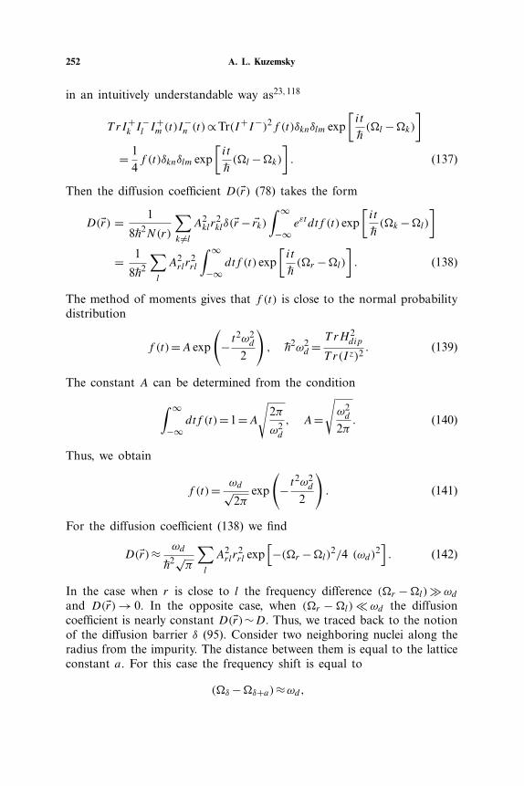
252 A. L. Kuzemsky
in an intuitively understandable way as23,118
T rI+k I
−l I
+m (t)I
−n (t)∝Tr(I+I−)2f (t)δknδlm exp
[it–h(�l −�k)
]
= 14f (t)δknδlm exp
[it–h(�l −�k)
]. (137)
Then the diffusion coefficient D(�r) (78) takes the form
D(�r) = 1
8–h2N(r)
∑k �=l
A2klr
2klδ(�r− �rk)
∫ ∞
−∞eεtdtf (t) exp
[it–h(�k −�l)
]
= 1
8–h2
∑l
A2rlr
2rl
∫ ∞
−∞dtf (t) exp
[it–h(�r −�l)
]. (138)
The method of moments gives that f (t) is close to the normal probabilitydistribution
f (t)=A exp
(− t
2ω2d
2
), –h2ω2
d =T rH 2
dip
T r(I z)2. (139)
The constant A can be determined from the condition
∫ ∞
−∞dtf (t)=1=A
√2π
ω2d
, A=√ω2d
2π. (140)
Thus, we obtain
f (t)= ωd√2π
exp
(− t
2ω2d
2
). (141)
For the diffusion coefficient (138) we find
D(�r)≈ ωd–h2√π
∑l
A2rlr
2rl exp
[−(�r −�l)2/4 (ωd)2
]. (142)
In the case when r is close to l the frequency difference (�r −�l)�ωdand D(�r)→ 0. In the opposite case, when (�r −�l)� ωd the diffusioncoefficient is nearly constant D(�r)∼D. Thus, we traced back to the notionof the diffusion barrier δ (95). Consider two neighboring nuclei along theradius from the impurity. The distance between them is equal to the latticeconstant a. For this case the frequency shift is equal to
(�δ −�δ+a)≈ωd,
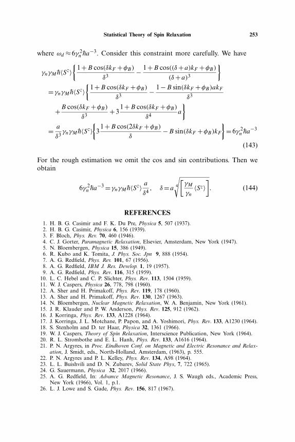
Statistical Theory of Spin Relaxation 253
where ωd ≈6γ 2n
–ha−3. Consider this constraint more carefully. We have
γnγM–h〈Sz〉
{1+B cos(δkF +φB)
δ3− 1+B cos((δ+a)kF +φB)
(δ+a)3}
=γnγM–h〈Sz〉{
1+B cos(δkF +φB)δ3
− 1−B sin(δkF +φB)akFδ3
+B cos(δkF +φB)δ3
+31+B cos(δkF +φB)
δ4a
}
= a
δ3γnγM
–h〈Sz〉{
31+B cos(2δkF +φB)
δ−B sin(δkF +φB)kF
}=6γ 2
n–ha−3
(143)
For the rough estimation we omit the cos and sin contributions. Then weobtain
6γ 2n
–ha−3 =γnγM–h〈Sz〉 aδ4, δ=a 4
√[γM
γn〈Sz〉
]. (144)
REFERENCES
1. H. B. G. Casimir and F. K. Du Pre, Physica 5, 507 (1937).2. H. B. G. Casimir, Physica 6, 156 (1939).3. F. Bloch, Phys. Rev. 70, 460 (1946).4. C. J. Gorter, Paramagnetic Relaxation, Elsevier, Amsterdam, New York (1947).5. N. Bloembergen, Physica 15, 386 (1949).6. R. Kubo and K. Tomita, J. Phys. Soc. Jpn 9, 888 (1954).7. A. G. Redfield, Phys. Rev. 101, 67 (1956).8. A. G. Redfield, IBM J. Res. Develop. 1, 19 (1957).9. A. G. Redfield, Phys. Rev. 116, 315 (1959).
10. L. C. Hebel and C. P. Slichter, Phys. Rev. 113, 1504 (1959).11. W. J. Caspers, Physica 26, 778, 798 (1960).12. A. Sher and H. Primakoff, Phys. Rev. 119, 178 (1960).13. A. Sher and H. Primakoff, Phys. Rev. 130, 1267 (1963).14. N. Bloembergen, Nuclear Magnetic Relaxation, W. A. Benjamin, New York (1961).15. J. R. Klauder and P. W. Anderson, Phys. Rev. 125, 912 (1962).16. J. Korringa, Phys. Rev. 133, A1228 (1964).17. J. Korringa, J. L. Motchane, P. Papon, and A. Yoshimori, Phys. Rev. 133, A1230 (1964).18. S. Stenholm and D. ter Haar, Physica 32, 1361 (1966).19. W. J. Caspers, Theory of Spin Relaxation, Interscience Publication, New York (1964).20. R. L. Strombothe and E. L. Hanh, Phys. Rev. 133, A1616 (1964).21. P. N. Argyres, in Proc. Eindhoven Conf. on Magnetic and Electric Resonance and Relax-
ation, J. Smidt, eds., North-Holland, Amsterdam, (1963), p. 555.22. P. N. Argyres and P. L. Kelley, Phys. Rev. 134, A98 (1964).23. L. L. Buishvili and D. N. Zubarev, Solid State Phys, 7, 722 (1965).24. G. Sauermann, Physica 32, 2017 (1966).25. A. G. Redfield, In: Advance Magnetic Resonance, J. S. Waugh eds., Academic Press,
New York (1966), Vol. 1, p.1.26. L. J. Lowe and S. Gade, Phys. Rev. 156, 817 (1967).
254 A. L. Kuzemsky
27. B. Robertson, Phys. Rev. 153, 391 (1967).28. J. Jeener, in Advance Magnetic Resonance, J. S. Waugh eds., Academic Press, New York
(1968), Vol. 3, p.206.29. P. R. Moran, J. Phys. Chem. Solids, 30, 297 (1969).30. H. Meyer, S. M. Myers, and J. P. Remeika, J. Phys. Chem. Solids, 30, 2687 (1969).31. H. Meyer, S. M. Myers, and J. P. Remeika, J. Phys. Chem. Solids, 32, 867 (1971).32. M. Goldman, Spin Temperature and Nuclear Magnetic Resonance in Solids, Oxford Uni-
versity Press, Oxford, New York (1970).33. A. Abragam, Principles of Nuclear Magnetism, Oxford University Press, Oxford, (1961).34. D. Wolf, Spin-temperature and Nuclear-spin Relaxation in Matter. Oxford University
Press, Oxford, New York (1979).35. C. P. Slichter, Principles of Magnetic Resonance, Springer, Berlin, (1980).36. G. J. Ehnholm, J. P. Ekstrom, J. F. Jacquinot, M. J. Loponen, O. V. Lounasmaa, and J.
K. Soini, J. Low Temp. Phys. 39, 417 (1980).37. A. Abragam and M. Goldman, Nuclear Magnetism: Order and Disorder, Oxford Uni-
versity Press, Oxford, New York (1982).38. G. S. Boutis, D. Greenbaum, H. Cho, D. G. Gory, and C. Ramanathan, Phys. Rev.
Lett. 92, 137201 (2004).39. W. K. Rhim, A. Pines, and J. S. Waugh, Phys. Rev. Lett. 25, 218 (1970).40. L. L. Buishvili, Zh. Exp. Th. Phys., 49, 1868 (1965).41. L. L. Buishvili, Solid State Phys, 7, 1871 (1965).42. N. S. Bendiashvili, L. L. Buishvili, and M. D. Zviadadze, Solid State Phys. 8, 2919
(1966).43. L. L. Buishvili and M. D. Zviadadze, Phys.Lett. A 25, 86 (1967).44. L. L. Buishvili and M. D. Zviadadze, Solid State Phys. 10, 2553 (1968).45. P. Borckmans and D. Walgraef, in Proc. XV Colloque Ampere, North-Holland, Amster-
dam (1969), p. 418.46. L. L. Buishvili and N. P. Giorgadze, Dokl Akad Nauk SSSR 189, 508 (1969).47. L. L. Buishvili, M. D. Zviadadze, and G. R. Khutsishvili, Zh. Exp. Th. Phys., 56, 290
(1969).48. L. L. Buishvili and N. P. Giorgadze, Solid State Phys 12, 1817 (1970).49. N. S. Bendiashvili, L. L. Buishvili, and M. D. Zviadadze, Zh. Exp. Th. Phys., 58, 597
(1970).50. L. L. Buishvili and N. P. Giorgadze, Dokl Acad Nauk SSSR 191, 58 (1970).51. N. G. Fazleev, Sov. J. Low Temp. Phys. 5, 181 (1979).52. N. G. Fazleev, Sov. J. Low Temp. Phys. 6, 693 (1980).53. D. Tayurskii, Phys. Stat. Sol.B 162, 545 (1989).54. R. Nigmatullin and D. Tayurskii, Physica A 175, 275 (1991).55. V. Romero-Rochin, A. Orsky, and I. Oppenheim, Physica A 156, 244 (1989).56. W. T. Grandy, Foundations of Statistical Mechanics: Equilibrium Theory, D. Reidel Pub-
lishing Doddrecht, Holland (1987), Vol. 1.57. W. T. Grandy, Foundations of Statistical Mechanics: Nonequilibrium Phenomena , D.
Reidel Publishing (Doddrecht Holland, (1988), Vol. 258. M. Toda, R. Kubo and N. Saito, Statistical Physics: Equilibrium Statistical Mechanics,
Springer Publishing Berlin, (1992), Vol. 1.59. R. Kubo, M. Toda, and N. Hashitsume, Statistical Physics: Nonequilibrium Statistical
Mechanics, Springer Publishig Berlin, (1991), Vol. 2.60. D. N. Zubarev, Nonequilibrium Statistical Thermodynamics, Consultant Bureau, New
York (1974).61. J. A. McLennan Introduction to Nonequilibrium Statistical Mechanics, Prentice Hall,
New Jersey, (1989).62. R. Zwanzig, Nonequilibrium Statistical Mechanics, Oxford University Press, Oxford,
New York (2001).63. J. L. Lebowitz, Physica A 263, 516 (1999).64. A. L. Kuzemsky, Intern. J. Modern Phys. B 19, 1029 (2005) (cond-mat/0502194).
Statistical Theory of Spin Relaxation 255
65. N. N. Bogoliubov, in Studies in Statistical Mechanics, J. de Boer and G. E. Uhlenbeck,eds., North-Holland, Amsterdam, (1962), Vol. 1, p.1.
66. N. N. Bogoliubov, On the stochastic processes in the dynamical systems”, Communica-tions E17-10514, JINR, Dubna (1977).
67. Z. Onyszkiewicz, Physica A 143, 287 (1987).68. M. Gell-Mann and M. L. Goldberger, Phys. Rev. 91, 398 (1953).69. N. N. Bogoliubov, Quasi-averages in the problems of statistical mechanics, Communica-
tions D-781, JINR, Dubna (1961).70. L. van Hove, Physica 23, 411 (1957).71. R. Zwanzig, Physica 30, 1109 (1964).72. A. Fulinski and W. J. Kramarczyk, Physica 39, 575 (1968).73. L. A. Pokrowsky, Dokl Acad Nauk SSSR 183, 806 (1968).74. R. I. Cukier and J. M. Deutch, J. Chem. Phys. 50, 36 (1969).75. P. Hubbard, Rev. Mod. Phys. 33, 249 (1961).76. G. R. Khutsishvili, Usp. Fiz. Nauk. 87, 211 (1965); Sov. Phys. Uspekhi, 8, 743 (1966).77. G. R. Khutsishvili Comment Solid State Phys. 5, 23 (1972).78. P. M. Morse and H. Feshbach, Methods of Theoretical Physics , McGraw-Hill Book
Co., New York (1953).79. G. Arfken, Mathematical Methods for Physicists, Academic Press New York (1985).80. J. P. Stark, Solid State Diffusion, Wiley, New York (1976).81. W. E. Blumberg, Phys. Rev. 119, 79 (1960).82. D. A. Rigney and C. P. Flynn, Phil. Mag. 15, 1213 (1967).83. E. C. Hirschkoff, O. G. Symko, and J. C. Wheatley, J. Low Temp. Phys. 5, 155 (1971).84. J. J. Peters and C. P. Flynn, Phys. Rev. B 6, 3343 (1972).85. K. Yoshida and T. Moriya, J. Phys. Soc. Jpn 11, 33 (1956).86. W. Kohn and S. H. Vosko, Phys. Rev. 119, 912 (1960).87. M. B. Walker, Phys. Rev. 176, 432 (1968).88. B. Giovannini and A. J. Heeger, Helv. Phys. Acta 42, 639 (1969).89. J. Solyom, Z. Phys. 238, 195 (1970).90. M. B. Walker, Phys. Rev. B 1, 3690 (1970).91. B. Giovannini, P. Pincus, G. Gladstone, and A. J. Heeger, J. Physique 32, C1-163
(1971).92. J. Zitkova-Wilcox, Solid State Commun. 12, 1109 (1973).93. P. Nozieres, J. Low Temp. Phys. 17, 31 (1974).94. N. Bloembergen and T. J. Rowland, Acta Metall. 1, 731 (1953).95. N. Bloembergen and T. J. Rowland, Phys. Rev. 97, 1679 (1955).96. T. J. Rowland, Phys. Rev. 119, 900 (1960).97. R. L. Streever, Phys. Rev. 134, A1612 (1964).98. S. Clough and W. I. Goldburg, J. Chem. Phys. 45, 4080 (1966).99. J. R. Asik, M. A. Ball, and C. P. Slichter, in Magnetic Resonance and Relaxation,
Proc. XIV Colloque Ampere, Ljubljana, 1966 R. Blinc, eds., North-Holland, Amsterdam(1967), p. 448.
100. O. J. Lumpkin, Phys. Rev. 164, 324 (1967).101. A. C. Gossard, A. J. Heeger, and J. H. Wernick, J. Appl. Phys. 38, 1251 (1967).102. R. E. Walstedt, R. C. Sherwood, and J. H. Wernick, J. Appl. Phys. 39, 555 (1968).103. R. E. Walstedt and A. Narath, Phys. Rev. B 6, 4118 (1972).104. M. I. Aaalto, P. M. Berglund, H. K. Collan, G. J. Ehnholm, R. G. Gylling, and O. V.
Lounasmaa, Physica 61, 314 (1972).105. D. C. Lo, D. V. Lang, J. B. Boyce, and C. P. Slichter, Phys. Rev. B 8, 973 (1973).106. H. Alloul and P. Bernier, J. Phys. F: Metal Phys. 4, 870 (1974).107. H. Alloul, J. Darville, and P. Bernier, J. Phys. F: Metal Phys. 4, 2050 (1974).108. P. Bernier and H. Alloul, J. Phys. F: Metal Phys. 6, 1193 (1976).109. R. E. Walstedt and L. R. Walker, Phys. Rev. B 9, 4857 (1974).110. Y. Yafet and V. Jaccarino, Phys. Rev. 133, A1630 (1964).111. M. A. Ruderman and C. Kittel, Phys. Rev. 96, 99 (1954).
256 A. L. Kuzemsky
112. A. L. Kuzemsky, Physica B 355, 318 (2005).113. J. H. Van Vleck, Phys. Rev. 74, 1168 (1948).114. B. Coqblin The Electronic Structure of Rare-Earth Metals and Alloys: the Magnetic
Heavy Rare-Earths, Academic Press New York, (1977).115. F. Lado, J. D. Memory and G. W. Parker, Phys. Rev. B 4, 1406 (1971).116. J. Korringa, Physica 16, 601 (1950).117. T. Moriya, J. Phys. Soc. Jpn . 18, 516 (1963).118. R. Kubo, in Fluctuation, Relaxation, and Resonance in Magnetic Systems Proc. Scot-
tish Universities Summer School, 1961, D. ter Haar, ed., Oliver and Boyd, Edinburgh(1962), p. 23.
119. R. Kubo, Hyperfine Interactions 8, 731 (1981).