1 IntroductionIn spatial analysis, the ordinary linear regression (OLR) model has been one of themost useful statistical methods to identify the nature of relationships among variables(for example, see Dobson, 1990). In this technique, a variable y, called the dependentvariable, is modeled as a linear function of a set of independent variables x1 , x2 , .:: , xp .Based on n observations ( yi ; xi 1 , xi 2 , .:: , xip ), (i � 1, 2, .:: , n), from a study region, themodel can be expressed as

yi � b0 �Xpk � 1

bk xik � Ei , (1)

where b0 b1 , .:: , bp are parameters, and E1 E2 , .:: , En are error terms which are generallyassumed to be independent normally distributed random variables with zero meansand constant variance s 2. In this model, each of the parameters can be thought of asthe `slopes' between one of the independent variables and the dependent variable. Theleast squares estimate of the parameter vector can be written as

b � � b0 b1 .:: bp �T � �XTX�ÿ1XTY , (2)

where

X �

1 x1 1 . . . x1p

1 x2 1 . . . x2p

..

. ... ..

.

1 xn 1 . . . xnp

0BBB@1CCCA, Y �

y1y2...

yn

0BBB@1CCCA. (3)

Statistical tests for spatial nonstationarity based on thegeographically weighted regression model

Yee LeungDepartment of Geography, Centre for Environmental Studies, and Joint Laboratory forGeoinformation Science, The Chinese University of Hong Kong, Shatin, Hong Kong;e-mail: yeeleung@cuhk.edu.hk

Chang-Lin Mei, Wen-Xiu ZhangSchool of Science, Xi'an Jiaotong University, Xi'an Shaanxi, 710049, People's Republic of ChinaReceived 23 November 1998; in revised form 12 April 1999

Environment and Planning A 2000, volume 32, pages 9 ^ 32

Abstract. Geographically weighted regression (GWR) is a way of exploring spatial nonstationarity bycalibrating a multiple regression model which allows different relationships to exist at different pointsin space. Nevertheless, formal testing procedures for spatial nonstationarity have not been developedsince the inception of the model. In this paper the authors focus mainly on the development ofstatistical testing methods relating to this model. Some appropriate statistics for testing the goodnessof fit of the GWR model and for testing variation of the parameters in the model are proposed andtheir approximated distributions are investigated. The work makes it possible to test spatial non-stationarity in a conventional statistical manner. To substantiate the theoretical arguments, somesimulations are run to examine the power of the statistics for exploring spatial nonstationarity andthe results are encouraging. To streamline the model, a stepwise procedure for choosing importantindependent variables is also formulated. In the last section, a prediction problem based on the GWRmodel is studied, and a confidence interval for the true value of the dependent variable at a newlocation is also established. The study paves the path for formal analysis of spatial nonstationarity onthe basis of the GWR model.

DOI:10.1068/a3162

Statistical properties of these estimates have been well studied and various hypothesistests have also been established.

It is important to note that the slopes (that is, the parameters) in the model inequation (1) are assumed to be universal across the study area. However, in many real-life situations, there is ample evidence for the lack of uniformity in the effects of space.Variation or spatial nonstationarity in relationships over space commonly exist inspatial data sets and the assumption of stationarity or structural stability over spacemay be highly unrealistic (for example, see Anselin, 1988; Fotheringham et al, 1996;Fotheringham, 1997). It is shown that, as stated in Brunsdon et al (1996), (a) relation-ships can vary significantly over space and a `global' estimate of the relationships mayobscure interesting geographical phenomena; (b) variation over space can be suffi-ciently complex that it invalidates simple trend-fitting exercises. So, when analyzingspatial data, we should consider such modeling strategies that take into account thiskind of spatial nonstationarity.

Over the years, some approaches have been proposed to incorporate spatial struc-tural instability or spatial drift into the models. For example, Anselin (1988; 1990) hasinvestigated regression models with spatial structural change. Casetti (1972; 1986),Jones and Casetti (1992), and Fotheringham and Pitts (1995) have studied spatialvariations by the expansion method. Cleveland (1979), Cleveland and Devlin (1988),Casetti (1982), Foster and Gorr (1986), Gorr and Olligschlaeger (1994), Brunsdon et al(1996; 1997), and Fotheringham et al (1997a; 1997b) have examined the followingvarying-parameter regression model:

yi � bi 0 �Xpk � 1

bik xik � Ei . (4)

Unlike the OLR model in equation (1), this model allows the parameters to vary inspace. However, this model in its unconstrained form is not implementable becausethe number of parameters increases with the number of observations. Hence, strategiesfor limiting the number of degrees of freedom used to represent variation of theparameters over space should be developed when the parameters are estimated.

There are several methods for estimating the parameters. For example, the methodof the spatial adaptive filter (Foster and Gorr, 1986; Gorr and Olligschlaeger, 1994)uses generalized damped negative feedback to estimate spatially varying parameters ofthe model in equation (4). However, this approach incorporates spatial relationshipsin a rather ad hoc manner and produces parameter estimates that cannot be testedstatistically. Locally weighted regression method and kernel regression method (forexample, see Cleveland, 1979; Casetti, 1982; Cleveland and Devlin, 1988; Clevelandet al, 1988; Brunsdon, 1995; Wand and Jones, 1995) focus mainly on the fit of thedependent variable rather than on spatially varying parameters. Furthermore, theweighting system depends on the location in the `attribute space' (Openshaw, 1993) ofthe independent variables. For a further review of the varying-parameter model, see,for instance, Gorr and Olligschlaeger (1994) and Brunsdon et al (1996).

Along this line of thinking, Brunsdon et al (1996; 1997) and Fotheringham et al(1997a; 1997b) suggested a so-called geographically weighted regression (GWR) tech-nique in which the parameters in equation (4) are estimated by a weighted least squaresprocedure, making the weighting system dependent on the location in geographicalspace and, therefore, allowing local rather than global parameters to be estimated. Thetypical output from a GWR model is a set of parameters that can be mapped in thegeographic space to represent nonstationarity or parameter `drift'.

Compared with other methods, the GWR technique appears to be a relativelysimple but useful geographically oriented method to explore spatial nonstationarity.

10 Y Leung, C-L Mei,W-X Zhang

Based on the GWR model, not only can variation of the parameters be explored, butsignificance of the variation can also be tested. Unfortunately, at present, only MonteCarlo simulation has been used to perform tests on the validity of the model. In thistechnique, under the null hypothesis that the global linear regression model holds, anypermutation of the observations ( yi ; xi 1 , xi 2 , .:: , xip ) (i � 1, 2, .:: , n) among the geo-graphical sampling points is equally likely to occur. The observed values of thestatistics proposed can then be compared with these randomization distributions andthe significance tests can be performed accordingly. The computational overhead ofthis method is, however, considerable, especially for a large data set. Also, because thevalidity of these randomization distributions is limited to the given data set, this inturn restricts the generality of the proposed statistics. The ideal way to test the model isto construct appropriate statistics and to perform the tests in a conventional statisticalmanner.

The purpose of this paper is to solve the problem in the context of classical hypoth-esis testing. Specifically, we want to entertain two basic questions associated with theGWR model. (1) Given a situation, how can we tell whether the GWR model describesthe data set significantly better than an OLR model? (2) Given that the GWR model isvalid, does each set of its parameters vary significantly across the study region?

It is necessary to answer the first question when the GWR technique is employedto analyze a given data set. A GWR model will certainly fit a given data set better thanan OLR model. However, from the practical point of view, the simpler a model, theeasier it can be applied and interpreted. If a GWR model does not perform signifi-cantly better than an OLR model, we would rather use the OLR model in practice,and therefore we can also know that there is no significant drift in any of the modelparameters. By answering the second question, we can specify which set of the param-eters drifts significantly over the study region.

In this paper we propose several appropriate statistics and derive their approxi-mated null distributions for the statistical test of the above hypotheses. We also extendthe stepwise procedure for the selection of independent variables in the OLR modelto the GWR model. Based on the statistics and their approximated distributions, wefurther consider the prediction aspect of the GWR model and derive the intervalestimate for the true value of the dependent variable at a new location.

We first introduce the GWR model and briefly describe the related problems insection 2. The goodness-of-fit tests based on the residual sum of squares for the GWRmodel and a stepwise procedure for choosing important independent variables areproposed in section 3. In section 4, we propose a statistical test to examine whethereach set of the parameters of the GWR model varies significantly across a studyregion. In section 5, simulations are performed to examine the power of the proposedstatistical methods, and in section 6, we consider the prediction problem of the GWRmodel and construct a confidence interval for the true value of the dependent variable.The paper is then concluded with a brief summary and discussion.

2 Geographically weighted regression2.1 The model and the estimation of the parametersThe mathematical presentation of the GWR model is the same as the varying-param-eter regression model in equation (4). Here, the parameters are assumed to be functionsof the locations on which the observations are obtained. That is,

yi � bi 0 �Xpk � 0

bik xik � Ei , i 2 C � f1, 2, .:: , ng , (5)

Statistical tests for spatial nonstationarity 11

where C is the index set of locations of n observations and bik is the value of the k thparameter at location i.

The parameters in the GWR model are estimated by the weighted least squaresapproach. The weighting matrix is taken as a diagonal matrix where each element in itsdiagonal is assumed to be a function of the location of observation. Suppose that theweighting matrix at location i is W(i ). Then the parameter vector at location i isestimated as

b�i � � �XTW�i �X�ÿ1XTW�i �Y , (6)

where W(i ) � diag[w1 (i ), w2 (i ), .:: , wn (i )] and X and Y are defined as in equation (3).Here we assume that the inverse of the matrix XTW(i )X exists.

In fact, according to the principle of the weighted least squares method, thegenerated estimators at location i in equation (6) are obtained by solving the followingoptimization problem. That is, determine the parameters b0 , b1 , .:: , bp at each loca-tion i so thatXn

j � 1

wj �i�� yj ÿ b0 ÿ b1xj 1 ÿ .::ÿ bp xjp �2 (7)

is minimized. Given appropriate weights wj (i ) which are a function of the locations atwhich the observations are made, different emphases can be given to different observa-tions for generating the estimated parameters at location i.

2.2 Possible choices of the weighting matrixAs pointed out above, the role of the weighting matrix is to place different emphaseson different observations in generating the estimated parameters. In spatial analysis,observations close to a location i are generally assumed to exert more influence on theparameter estimates at location i than those farther away. When the parameters atlocation i are estimated, more emphasis should be placed on the observations whichare close to location i. A simple but natural choice of the weighting matrix at location iis to exclude those observations that are farther than some distance d from location i.This is equivalent to setting a zero weight on observation j if the distance from i to j isgreater than d. If the distance from i to j is expressed as dij , the elements of theweighting matrix at location i can be chosen as

wj �i � �1; if dij 4 d , j � 1, 2, .:: , n .

0; if dij > d;

((8)

The above weighting function suffers from the problem of discontinuity over thestudy area. One way to overcome this problem is to specify wj (i ) as a continuous andmonotone decreasing function of dij . One obvious choice might be

wj �i � � exp�ÿyd 2ij �, j � 1, 2, .:: , n , (9)

so that, if i is a point at which observation is made, the weight assigned to thatobservation will be unity and the weights of the others will decrease according toa Gaussian curve as dij increases. Here, y is a nonnegative constant depicting theway the Gaussian weights vary with distance. Given dij , the larger y, the less emphasisis placed on the observation at location j. The problem of equation (9) amounts toassigning weights to all locations of the study area.

A compromise between the above two weighting functions can be reached by settingthe weights to zero outside a radius d and to decrease monotonically to zero inside theradius as dij increases. For example, we can take the elements of the weighting matrix as

12 Y Leung, C-L Mei,W-X Zhang

a bisquare function, that is,

wj �i � ��1ÿ d 2

ij=d2�2; if dij 4 d , j � 1, 2, .:: , n ,

0; if dij > d;

((10)

The weighting function in equation (9) is the most common choice in practice.

2.3 Estimation of the parameter in the weighting matricesIn the process of calibrating a GWR model, the weighting matrix should first bedecided. If we use, for example, Gaussian weighting in equation (9), the parameter yshould be predetermined. This can be done by a cross-validation procedure (for exam-ple, see Cleveland, 1979; Bowman, 1984; Brunsdon, 1995). Let

D�y� �Xni � 1

� yi ÿ y�i � �y��2 , (11)

where y�i � (y) is the fitted value of yi with the observation at location i omitted from thecalibration process. Choose y0 as a desirable parameter such that

D�y0 � � minD�y� . (12)

In practice, plotting D(y) against the parameter y will provide guidance on selectingan appropriate value of the parameter or it can be selected automatically by anoptimization technique. The parameter in other forms of the weighting matrix can bedetermined similarly.

2.4 Testing for spatial nonstationarity of the parameters in the modelThe importance of exploring spatial nonstationarity has been fully addressed by, forexample, Fotheringham et al (1997b) and Charlton et al (1997). The GWR techniquehas been demonstrated to be a useful means for detecting spatial nonstationarity. Byknowing whether or not the parameters in a GWR model vary significantly, we canprovide not only a greater insight into both the data and the framework in which thedata are examined, but also some valuable guidance for decision in future actions.

From the statistical point of view, the following two questions are the mostimportant and should be tested statistically:(1) Does a GWR model describe the data significantly better than an OLR model?That is, on the whole, do the parameters in the GWR model vary significantly over thestudy region?(2) Does each set of parameters bik (i � 1, 2, .:: , n) exhibit significant variation overthe study region?

For the first question, it is, in fact, a goodness-of-fit test for a GWR model. It isequivalent to testing whether or not y � 0 if we use equation (9) as the weightingfunction. In the second case, for any fixed k, the deviation of bik (i � 1, 2, .:: , n) canbe used to evaluate the variation of the slope of the k th independent variable. Becauseit is very difficult to find the null distribution of the estimated parameter, say y inequation (9), in the weighting matrix, a Monte-Carlo technique has been employed toperform the tests (Brunsdon et al, 1996; Fotheringham et al, 1997a). However, aspointed out above, the computational overhead of the method is considerable. Further-more, the validity of the reference distributions obtained by the randomized permutationis limited to the given data set, and it in turn may restrict the generality of thecorresponding statistics.

Some other approaches which account for spatial variation tend to add extra param-eters to the model. For example, the structural change models examine spatial variationby dividing the study area into several regions and calibrating different regression modelsin different regions (for example, see Anselin, 1988; 1990); the expansion method embeds

Statistical tests for spatial nonstationarity 13

spatial variation by assuming the regression coefficients to be the other function of thelocations (for example, see Jones and Casetti, 1992; Fotheringham and Pitts, 1995). Inthese cases, the number of parameters in the model is fixed and the classical likelihoodratio tests can therefore be used to test spatial nonstationarity. For the varying-parameterregression model in equation (1), the number of parameters in the model, as has beenpointed out in section 1, increases with the number of observations. The GWR techniquein fact exerts some constraints on the parameters by the weighted least squares method.Given the way parameters in the GWRmodel are estimated, it is unlikely to base the testson the likelihood function to test spatial nonstationarity. However, it is still correct toperform the tests by using the residuals.

In the following two sections we use the notion of residual sum of squares toformulate some methods to examine the above questions within the conventionalhypothesis-testing framework. Based on the proposed statistics and their approximateddistributions, we also propose a stepwise procedure for choosing important independ-ent variables of the GWR model.

3 Goodness-of-fit test and stepwise procedure for selection of independent variablesBased on the notion of residual sum of squares, some statistics are constructed in thissection, and their approximated distributions are investigated to test whether a GWRmodel describes a given data set significantly better than an OLR model does. Ourderivation is an extension of the method described in Cleveland and Devlin (1988)and Cleveland et al (1988). Furthermore, we propose a stepwise procedure to chooseimportant independent variables within the framework of the GWR model.

In the sections to follow, we assume that the weighting matrix for calibrating theGWR model is given and the following two assumptions hold:

Assumption 1. The error terms E1 , E2 , .:: , En are independently identically distributed asa normal distribution with zero mean and constant variance s 2.

Assumption 2. Let yi be the fitted value of yi at location i. For all i � 1, 2, .:: , n, yi isan unbiased estimate of E( yi ). That is, E( yi ) � E( yi ) for all i.

Assumption 1 is in fact the conventional assumption in theoretical analysis ofregression. Assumption 2 is in general not exactly true for local linear fitting exceptthat the exact global linear relationship between the dependent variable and the inde-pendent variables exists (see Wand and Jones, 1995, page 120 ^ 121 for the univariatecase). However, the local-regression methodology is mainly oriented towards the searchfor low-bias estimates (Cleveland et al, 1988). In this sense, the bias of the fitted valuecould be negligible So, assumption 2 is a realistic one in the GWR model because thistechnique still belongs to the local-regression methodology.

3.1 The residual sum of squares and its approximated distributionLet xT

i � (1 xi 1 .::xip ) be the i th row of X (i � 1, 2, .:: , n) and b(i ) the estimatedparameter vector at location i. Then the fitted value of yi is given by

yi � xTi b�i � � xT

i �XTW�i �W�ÿ1XTW�i �Y . (13)

Let Y � ( y1 y2 .:: yn )T be the vector of the fitted values and let EE � (E1 E2 .:: En )

T be thevector of the residuals. Then

Y � LY , (14)

EE � Yÿ Y � �Iÿ L�Y , (15)

14 Y Leung, C-L Mei,W-X Zhang

where

L �

xT1 �XTW�1�X�ÿ1XTW�1�

xT2 �XTW�2�X�ÿ1XTW�2�

..

.

xTn �XTW�n�X�ÿ1XTW�n�

0BBBBB@

1CCCCCA (16)

is an n� n matrix and I is an identity matrix of order n.It should be noted that the role of the matrix L is to turn the observed values of the

dependent variable into the fitted ones, which is the same as that of the hat matrix inthe OLR literature (for example, see Neter et al, 1989). However, the hat matrix in theOLR literature is symmetric and idempotent, but, because of the weighting matrixW(i ) (i � 1, 2, .:: , n), L is generally not.

We denote by RSSg the residual sum of squares. Then

RSSg �Xni � 1

E 2i � EETEE � Y T�Iÿ L�T�Iÿ L�Y . (17)

This quantity measures the goodness of fit of a GWR model for the given data and canbe used to estimate s 2, the common variance of the error terms Ei (i � 1, 2, .:: , n).Indeed, according to assumptions 1 and 2, we have

E�EE� � E�Y � ÿ E�Y � � 0, E�EEEET � � s 2 I , (18)

where EE � (E1 E2 .:: En �T is the vector of the error terms. Therefore, RSSg can also beexpressed as

RSSg � �EEÿ E�EE��T �EEÿ E�EE��� �Yÿ E�Y ��T�Iÿ L�T�Iÿ L��Yÿ E�Y ��� EET�Iÿ L�T�Iÿ L�EE . (19)

So,

E�RSSg� � E�EET�Iÿ L�T�Iÿ L�EE�� Eftr�EET�Iÿ L�T�Iÿ L�EE�g� Eftr��Iÿ L�T�Iÿ L�EEEET �g� tr��Iÿ L�T�Iÿ L�E�EEEET��� s 2d1 , (20)

where d1 � tr��Iÿ L�T�Iÿ L��. From equation (20) we know that

s 2 � RSSg

d1(21)

is an unbiased estimate of s 2. From equation (19) RSSg can be represented as aquadratic form of normal variables with a symmetric and positive semidefinite matrix�Iÿ L�T�Iÿ L�. It is well know that a quadratic form of standardized normal variablesnTA n [that is, n� N(0, I� and A is symmetric] is distributed as w 2 distribution if andonly if A is idempotent (for example, see Johnson and Kotz, 1970, chapter 29; Stuartand Ord, 1994, chapter 15). For the random variable

RSSg

s 2��EEs

�T�Iÿ L�T�Iÿ L� EE

s, (22)

Statistical tests for spatial nonstationarity 15

although EE=s � N(0, I), the matrix �Iÿ L�T�Iÿ L� is generally not idempotent becauseof the complexity of the weighting matrix W(i ) (it is different at each location i ).Therefore RSSg=s

2 is generally not distributed as an exact w 2 distribution. However,there are several ways to approximate the distribution of the quadratic form nTA n withnormal variables n (for example, see Johnson and Kotz, 1970, chapter 29 and the relatedreferences; Solomon and Stephens, 1977; 1978; Stuart and Ord, 1994, chapter 15). Onesimple but accurate method is to approximate the distribution of this quadratic formby that of a constant c multiplied by a w 2 variable w 2

r with r degrees of freedom if thematrix A is symmetric and positive semidefinite, where c and r are chosen in such away that the first two moments of cw 2

r are made to agree with those of the quadraticform, or equally, the mean and variance of cw 2

r and those of the quadratic form aremade to match each other. We know from equation (20) that the mean of RSSg=s

2 isd1 . Using our knowledge of matrix algebra, we can obtain the variance of RSSg =s

2

as 2d2 (see appendix A), where

d2 � tr��Iÿ L�T�Iÿ L��2 . (23)

It is a standard result that the mean and the variance of the random variable w 2r are r

and 2r, respectively. So, the mean and variance of cw 2r are cr and 2c 2r, respectively.

According to the approximating rule stated above, let

cr � d1 ;

2c 2r � 2d2 :

((24)

Solving the equations, we obtained c � d2=d1 , and r � d 21 =d2 . So, the distribution of

RSSg=cs2 � d 2

1 s2=d2s

2 can well be approximated by a w 2 distribution with d 21 =d

2

degrees of freedom.

3.2 Testing for goodness of fitUsing the residual sum of squares and its approximated distribution, we can testwhether a GWR model describes a given data set significantly better than an OLRmodel does. If a GWR model is used to fit the data, under assumption 2, the residualsum of squares can be expressed as RSSg � YT(Iÿ L)T(Iÿ L)Y, and the distributionof d1RSSg=d2s

2 can well be approximated by a w 2 distribution with d 21=d2 degrees of

freedom. If an OLR model is used to fit the data, the residual sum of squares isRSSo � YT(IÿQ)Y, where Q � X(XTX)ÿ1XT, and IÿQ is idempotent. So,RSSo=s

2 is exactly distributed as a w 2 distribution with nÿ pÿ 1 degrees of freedom(for example, see Neter et al, 1989; Hocking, 1996).

If the null hypothesisöH0: there is no significant difference between OLR andGWR models for the given dataöis true, the quantity RSSg=RSSo is close to one.Otherwise, it tends to be small. Let

F1 �RSSg=d1

RSSo=�nÿ pÿ 1� . (25)

Then a small value of F1 supports the alternative hypothesis that the GWR model hasa better goodness of fit. On the other hand, the distribution of F1 may reasonably beapproximated by an F-distribution with d 2

1 =d2 degrees of freedom in the numeratorand nÿ pÿ 1 degrees of freedom in the denominator. Given a significancelevel a, we denote by F1ÿa (d

21=d2 , nÿ pÿ 1) the upper 100(1ÿ a) percentage point. If

F1 < F1ÿa (d21=d2 , nÿ pÿ 1), we reject the null hypothesis and conclude that the GWR

model describes the data significantly better than the OLR model does. Otherwise, wewill say that the GWR model cannot improve the fit significantly compared with theOLR model.

16 Y Leung, C-L Mei,W-X Zhang

Another possibility to test the goodness of fit is to use the method of analysis ofvariance. Let

DSS � RSSo ÿRSSg � YT��IÿQ� ÿ �Iÿ L�T�Iÿ L��Y � YTAY , (26)

where A, A � (IÿQ)ÿ (Iÿ L)T(Iÿ L), is positive semidefinite because DSS 5 0 forany Y. This quantity measures the difference of the residual sums of squares. If theGWR model cannot significantly improve the goodness of fit compared with the OLRmodel, the quantity DSS must be sufficiently small. Under assumption 1 and the nullhypothesis that the GWR model and the OLR model describe the data equally well,we can assume that the fitted values of yi by the GWR model and the OLR modelare all unbiased estimates of E( yi ) for all i. Therefore, by the aforementionedmethod, DSS can be expressed as DSS � EETAEE and the distribution of n1DSS=n2s

2

can be approximated by a w 2 distribution with n 21=n2 degrees of freedom, where

ni � tr(Ai ) (i � 1; 2). Using this fact, we can construct a test statistic as follows:

F2 �DSS=n1

RSSo=�nÿ pÿ 1� . (27)

A small value of F2 will support the null hypothesis. Once again, the distribution of F2

may be approximated by an F-distribution with n 21=n2 degrees of freedom in the

numerator and nÿ pÿ 1 degrees of freedom in the denominator. Given a significancelevel a, we reject the null hypothesis if F2 > Fa (n

21=n2 ; nÿ pÿ 1), where

Fa (n21 =n2 ; nÿ pÿ 1) is the upper 100a percentage point of the F-distribution.For simplicity of calculation, n1 and n2 can be expressed in a more explicit way.

Indeed, it is easy to prove that (see the detailed proof in appendix B)

LQ � Q ,

A 2 � �IÿQ� ÿ 2�Iÿ L�T�Iÿ L� � ��Iÿ L�T�Iÿ L��2:

((28)

Therefore, we have

n1 � tr�A� � nÿ pÿ 1ÿ d1 ;

n2 � tr�A2� � nÿ pÿ 1ÿ 2d1 � d2 :

((29)

3.3 A stepwise procedure for the selection of independent variablesIn practice, we frequently suspect that a large number of independent variables mighthave some effect on the dependent variable. Nevertheless, too many independentvariables included in the model make the explanation of the model superfluous andthe computation unnecessarily complex. Furthermore, simulation results in Clevelandet al (1988) showed that the distributional approximations proposed above performswell when the number of independent variables in the model is small, but this approxi-mation may become poor as the number of independent variables increases. So, it isessential to choose in the model calibration process independent variables that areimportant and exclude those that are less important.

An independent variable is said to be important if the residual sum of squares issignificantly reduced when it is added to the model. Taking the ratio of the residualsums of squares before and after an independent variable is added to the model as ameasurement of the change in the residual sum of squares due to the model, wepropose a stepwise procedure for choosing important independent variables in calibrat-ing a GWR model. The procedure is, to some extent, similar to that used in thebuilding of an OLR model (for example, see Neter et al, 1989). It is a combinedutilization of the forward selection procedure and the backward elimination procedure

Statistical tests for spatial nonstationarity 17

parallel to that of the OLR model. To facilitate our discussion, we first propose anddiscuss the forward and backward procedures.

The forward selection procedure can be structured as follows.(1) Fit a GWR model with only the intercept terms as follows:

yi � bi 0 � Ei . (30)

For a given weighting matrix, the parameters are estimated by equation (6) and theresidual sum of squares is calculated by equation (17). In this special case, the esti-mated parameters are given by

bi 0 �Xnj � 1

wj �i �yj�Xn

j � 1

wj �i �, i � 1, 2, .:: , n , (31)

and the residual sum of squares is given by

RSS�0� � YT�Iÿ L�0��T�Iÿ L�0��Y, (32)

where

L�0� �

w1 �1�Pwj �1�

w2 �1�Pwj �1�

. . .wn �1�Pwj �1�

w1 �2�Pwj �2�

w2 �2�Pwj �2�

. . .wn �2�Pwj �2�

. . . . . . . . . . . .

w1 �n�Pwj �n�

w2 �n�Pwj �n�

. . .wn �n�Pwj �n�

0BBBBBBBBBB@

1CCCCCCCCCCA, j � 1, 2, .:: , n . (33)

(2) Let x1 , x2 , .:: , xp be all the candidate independent variables. For each xk , fit thefollowing model:

yi � bi 0 � bik xik � Ei . (34)

The parameters are still estimated by equation (6), but now X is an n� 2 matrix withall of the elements in the first column being 1 and the second column being the nobservations of xk . Calculate the residual sum of squares RSS(xk ) from

RSS�xk � � YT�Iÿ L�xk ��T�Iÿ L�xk ��Y, (35)

where L(xk ) is similar to equation (16) in which the matrix X and the correspondingrow vectors xT

i (i � 1, 2, .:: , n) have to be changed to the corresponding matrix statedabove.(3) For each k � 1, 2, .:: , p, calculate the following quantity

R�xk � �RSS�xk �=d1 �xk �RSS�0�=d1 �0�

, k � 1, 2, .:: , p , (36)

where

di �xk � � trf�Iÿ L�xk ��T�Iÿ L�xk ��gi;di �0� � trf�Iÿ L�0��T�Iÿ L�0��gi;

(i � 1, 2 . (37)

If adding xk to the model in equation (30) does not reduce the residual sum of squaressignificantly, that is, the models in equations (30) and (34) fit the data equally well, wemay assume that the mean of the fitted values of yi in model (30) and in model (34) areall equal to E( yi ). Under this assumption, as aforementioned, the distribution of eachR(xk ) can be approximated by the distribution F [d 2

1 (xk )=d2 (xk ), d21 (0)=d2 (0)]. Unlike

the statistics for choosing independent variables in the OLR model, the degrees of

18 Y Leung, C-L Mei,W-X Zhang

freedom of the approximated distributions of R(xk ) are related to xk (k � 1, 2, .:: , p).So, the curves of the approximated distribution functions are different from oneanother. In this case, it is inappropriate to choose important xk by comparing thequantity of R(xk ) because the smallest R(xk ) does not necessarily correspond to themost significant reduction in the residual sum of squares. But we may use the socalled p-values of the statistics to choose important independent variables. In thiscase, the p-value of R(xk ) is the probability that a random variable distributed asF [d 2

1 (xk )=d2 (xk ), d21 (0)=d2 (0)] takes on the value less than or equal to the observed

value of R(xk ) (the general concept of p-value will be further explained in section 5).Let xk be a random variable with distribution F [d 2

1 (xk )=d2 (xk ), d21 (0)=d2 (0)]. For

each k � 1, 2, .:: , p, calculate the p-values:

pk � P�xk 4 R�xk ��, k � 1, 2, .:: , p . (38)

Suppose

pk0� min

1 4 k 4 pf pkg . (39)

For a given significance level a, if pk0 < a, we first choose xk0to enter the model. The

reason is that the smallest p-value corresponds to the most significant reduction in theresidual sum of squares. Otherwise, there are no independent variables which can beregarded as important for enhancing the fit of the GWR model.(4) Under the condition of pk0 < a, add each of the xk (k 6� k0 ) to the model

yi � bi 0 � bik0xik0� Ei . (40)

Calibrate the model and calculate the residual sum of squares

RSS�xk0, xk � � YT�Iÿ L�xk0

, xk ��T�Iÿ L�xk0, xk ��Y, k 6� k0 . (41)

Let

R�xk0, xk � �

RSS�xk0, xk �=d1 �xk0

, xk �RSS�xk0

�=d1 �xk0� , k 6� k0 , (42)

where the meanings of L(xk0, xk ), di (xk0

, xk ), etc are similar to those in the previousdiscussion. Compute the p-values

pk � P�xk 4 R�xk0, xk ��, k 6� k0 , (43)

where xk (k 6� k0 ) is distributed as

F

�d 21 �xk0

, xk �d2 �xk0

, xk �;d 21 �xk0

�d2 �xk0

��. (44)

Letpk1� min

k 6� k0

f pkg . (45)

If pk1 < a, enter xk1into the model in equation (40). Otherwise, equation (40) is the

final model.Repeat step 4 until no independent variables among the candidate variables can be

entered into the model, and the model at this point is the final model.The main advantage of this procedure is its simplicity of calculation. The disadvan-

tage of it is that, once a variable has been entered into the model, it stays in the modelforever. In fact, when another variable enters the model afterwards, the variablespreviously entered may become insignificant in reducing the residual sum of squares.The method thus does not take into account the change in importance because of theswitch in entrance order.

Statistical tests for spatial nonstationarity 19

Unlike the forward selection procedure, the backward elimination procedure worksas follows. A GWR model which includes all of the candidate independent variables iscalibrated first. Then, the less important independent variables are eliminated one byone according to their significance in reducing the sum of squares with and without thevariable entered into the model. That is, we first fit the model

yi � bi 0 �Xpm � 1

bim xim � Ei . (46)

The residual sum of squares is given by

RSS�x1 , x2 , .:: , xp � � YT�Iÿ L�x1 , x2 , .:: , xp ��T�Iÿ L�x1 , x2 , .:: , xp ��Y . (47)

Then for each k � 1, 2, .:: , p, fit the model

yi � bi 0 �Xpm � 1m 6� k

bim xim � Ei . (48)

Its residual sum of squares is

RSS�x1 , .:: , xkÿ1 , xk�1 , .:: , xp �� YT�Iÿ L�x1 , .:: , xkÿ1 , xk�1 , .:: , xp ��T�Iÿ L�x1 , .:: , xkÿ1 , xk�1 , .:: , xp ��Y. (49)

Calculate

R�xk � �RSS�x1 , .:: , xp �=d1 �x1 , .:: , xp �

RSS�x1 , .:: , xkÿ1 , xk�1 , .:: , xp �=d1 �x1 , .:: , xkÿ1 , xk�1 , .:: , xp �, (50)

where

di �x1 , x2 , .:: , xp � � trf�Iÿ L�x1 , x2 , .:: , xp ��T�Iÿ L�x1 , x2 , .:: , xp ��gi,di �x1 , .:: , xkÿ1 , xk�1 , .:: , xp �� trf�Iÿ L�x1 , .:: , xkÿ1 , xk�1 , .:: , xp ��T�Iÿ L�x1 , .:: , xkÿ1 , xk�1 , .:: , xp ��gi ,

8><>: (51)

and i � 1, 2.Like the forward selection procedure, we still use the p-value of R(xk ) as a standard

to choose independent variables. Calculate the probability

pk � P�xk 4 R�xk �� , (52)

where xk is a random variable distributed as

F

�d 21 �x1 , .:: , xp �d2 �x1 , .:: , xp �

,d 21 �x1 , .:: , xkÿ1 , xk�1 , .:: , xp �

d2 �x1 , .:: , xkÿ1 , xk�1 , .:: , xp ��. (53)

Suppose

pk0� max

1 4 k 4 pf pkg . (54)

For a given significance level a, if pk0 5 a, then remove xk0from the model in equation

(46). Otherwise, keep all the independent variables in the model. This process isrepeated until no variables can be eliminated. The drawback of this method is that,once a variable has been deleted, it cannot reenter the model. Again, the order ofdeleting is not dealt with in this method.

The drawbacks of the forward selection and backward elimination procedures canbe overcome by a stepwise procedure parallel to that in OLR. It is actually a combina-tion of the two procedures just described. It starts with the model in equation (30) andselects variables one by one to enter the model in the manner of the forward selectionprocedure. But once a new variable has been entered into the model, the variables that

20 Y Leung, C-L Mei,W-X Zhang

have been entered in the previous steps are checked one by one again for theirsignificance in the manner of the backward elimination procedure. When a previouslyentered variable becomes insignificant, it will be eliminated. Otherwise, it will be keptin the model. This process is repeated until no other variables can be added to themodel and also no variables can be deleted from the model.

Remark. In practical applications, the parameter in the weighting matrix may beunknown. This parameter should be determined before the procedure for choosingimportant variables is performed. In this case, we may first fit a GWR model withall the candidate independent variables and estimate the parameter in the weightingmatrix by the cross-validation approach stated in section 2.3. After the process ofchoosing important independent variables has been completed, the cross-validationmethod is used again to refine this parameter, but now the model used includes onlythose independent variables that have been chosen. After redetermining the parameterin the weighting matrix, we can fit such a GWR model that includes only theimportant independent variables as our final model.

Given that the main purpose of the GWR technique is to explore spatial non-stationarity among the model parameters, the proposed stepwise methods may bethought of as a by-product when we can find the approximated distribution of theratio of residual sum of squares. These model selection methods are useful when thefitted model is used for explanation and prediction. On the other hand, from theexploration point of view, these methods may also be used for certain exploratoryanalysis because the process of selecting an independent variable is indeed the test ofwhether or not the coefficient of this variable is zero. If a variable is not included in theselected model, it means that the coefficient of this independent variable is not onlyconstant but is also zero at some significance level.

4 Test for variation of each set of parametersAfter a final model has been selected, we can further test whether or not each set ofparameters in the model varies significantly across the study region. For example, ifthe set of parameters fbik ; i � 1, 2, .:: , ng of xk (if k � 0, the parameters examinedcorrespond to the intercept terms) is tested not to vary significantly over the region, wecan treat the coefficient of xk to be constant and conclude that the slope between xk

and the dependent variable is uniform over the area when the other variables are takento be fixed. Statistically, it is equivalent to testing the hypotheses

H0 : b1k � b2k � .:: � bnk for a given k ,

H1 : not all bik �i � 1, 2, .:: , n� are equal .

First, we must construct an appropriate statistic which can reflect the spatial variation ofthe given set of parameters. A practical and yet natural choice is the sample varianceof the estimated values of bik (i � 1, 2, .:: , n) (Brunsdon et al, 1996; 1997). We denoteby V 2

k the sample variance of the n estimated values, bik (i � 1, 2, .:: , n) for the k thparameter. Then

V 2k � 1

n

Xni � 1

�bik ÿ

1

n

Xni � 1

bik

�2, (55)

where bik (i � 1, 2, .:: , n) are obtained from equation (6).The next stage is to determine the sampling distribution of V 2

k under the nullhypotheses H0 . Let bk � (b1k b2k .:: bnk )

T and let J be an n� n matrix with unity for

Statistical tests for spatial nonstationarity 21

each of its elements. Then V 2k can be expressed as

V 2k � 1

nb

T

k

�Iÿ 1

nJ

�bk . (56)

Under the null hypothesis that all the bik (i � 1, 2, .:: , n) are equal, we may assumethat the means of the corresponding estimated parameters are equal, that is,

E�b1k � � E�b2k � � .:: � E�bnk � � mk . (57)

So,

E�bk � � mk1 , (58)

where 1 is a column vector with unity for each element. From equation (58) and thefact that 1T(Iÿ 1

nJ) � 0 and (Iÿ 1

nJ)1 � 0, we can further express V 2

k as

V 2k � 1

n�bk ÿ E�bk ��T

�Iÿ 1

nJ

��bk ÿ E�bk �� . (59)

Furthermore, let ek be a column vector with unity for the (k� 1)th element and zerofor other elements. Then

bik � eTk b�i � � eT

k �XTW�i �X�ÿ1XTW�i �Y , (60)

and

bk � �b1k b2k .:: bnk �T � BY , (61)

where

B �

eTk �XTW�1�X�ÿ1XTW�1�eTk �XTW�2�X�ÿ1XTW�2�

..

.

eTk �XTW�n�X�ÿ1XTW�n�

0BBBBB@

1CCCCCA . (62)

Substituting equation (61) into equation (59), we obtain

V 2k � 1

n�Yÿ E�Y ��TBT

�Iÿ 1

nJ

�B�Yÿ E�Y ��

� EET�1

nBT

�Iÿ 1

nJ

�B

�EE , (63)

where EE � N(0, s 2I), and 1nBT�Iÿ 1

nJ�B is positive semidefinite.

Similar to the method employed in section 3, the distribution of g1V2

k =g2s2 can be

approximated by a w 2 distribution with g 21 =g2 degrees of freedom, where

gi � tr�1

nBT

�Iÿ 1

nJ

�B

�i, i � 1, 2 . (64)

Because s 2 is unknown, we cannot use g1V2k =g2s

2 as a test statistic directly. But fromsection 3, we know that the distribution of d 2

1 s2=d2s2 can be approximated by a w 2

distribution with d 21 =d2 degrees of freedom, where s 2 is an unbiased estimator of s 2

which is defined by equation (21), and di � tr[(Iÿ L)T(Iÿ L)]i (i � 1, 2). So, for thestatistic

F3 �k� �V 2

k =g1s 2

, (65)

22 Y Leung, C-L Mei,W-X Zhang

under the assumption in equation (57), its distribution can be approximated by anF-distribution with g 2

1 =g2 degrees of freedom in the numerator and d 21=d2 degrees of

freedom in the denominator. Therefore, we can take F3 as a test statistic. The largevalue of F3 supports the alternative hypothesis H1. For a given significance level a, findthe upper 100a percentage point Fa (g

21 =g2 , d

21=d2 ). If F3 5 Fa (g

21 =g2 , d

21=d2 ), reject H0;

accept H0 otherwise.

5 SimulationsIn this section, several simulated data sets with known parameters are used to examinethe test power of the statistics proposed in sections 3 and 4.

The models for generating the data sets are taken from Foster and Gorr (1986)where the data were used to compare the percentage improvement in fit and bias of thespatial adaptive filter over the ordinary least squares regression estimates. The spatialregion of parameter variation consists of coordinates (zi 1 , zi 2 ) taken from a uniform,two-dimensional grid consisting of m�m lattice points with unit distance betweenany two of them along the horizontal and vertical axes (as illustrated in figure 1).That is, the points for taking the observations are at the following lattice points:

f�zi 1 , zi 2 �; zi 1 , zi 2 � 0, 1, 2, .:: , mÿ 1g . (66)

The general form of the model being simulated is as follows:

yi � bi 0 � bi 1xi � Ei , (67)

where Ei � N(0, 4). The values of the independent variable x are drawn randomly from auniform distribution on interval (0, 1) and therefore contain no information on spatialvariation of parameters. Besides the five particular cases in Foster and Gorr (1986), twoother cases (linear change in both the intercept and slope, and step change in both theintercept and slope) are also considered. We list these seven cases as follows:Case 1. Stationary: bi 0 � 10; bi 1 � 15.Case 2. Linear change in intercept: bi 0 � 8:333� 1:667zi 1 ; bi 1 � 10.Case 3. Linear change in slope: bi 0 � 5; bi 1 � 12:5� 2:5zi 1 .Case 4. Linear change in both intercept and slope: bi 0 � 8:333� 1:667zi 1 ;bi 1 � 12:5� 2:5zi 1 .Case 5. Step change in intercept: bi 0 � 10 if zi 1 < � m2 �, and bi 0 � 15 otherwise, where� m2� represents the integer part of m

2; bi 1 � 10.

Case 6. Step change in slope: bi 0 � 5; bi 1 � 20 if zi 1 < � m2 �, and bi 1 � 30 otherwise.Case 7. Step change in both intercept and slope: bi 0 � 10 if zi 1 < � m2 �, and bi 0 � 15otherwise; bi 1 � 20 if zi 1 < � m2 �, and bi 1 � 30 otherwise.

unitdistance

6

5

4

3

2

1

observation points

z1

0 1 2 3 4 5 6

z 2

unit distance

Figure 1. A grid for generating the simulation data set: (the case of m � 7).

Statistical tests for spatial nonstationarity 23

In each case, we take m � 6, 7, 8, 9, 10 and perform the simulations. For a given m,the values xi are drawn from the uniform distribution on interval (0, 1); the error termsEi (i � 1, 2, .:: , m 2 ) are drawn from N(0, 4) and the corresponding values of thedependent variable yi are generated by the model in equation (67). The Gaussianweighting function in equation (9) is used and the parameter y in the weightingfunction is first determined by the cross-validation approach stated in section 2.3.Then, we fit the GWR model and calculate the values of the test statistics F1 inequation (25), F2 in equation (27), F3 (k) in equation (65) and the corresponding degreesof freedom.We use the p-values of the statistics to show the degree of significance. Fora one-tailed test, the p-value of the test statistic is the probability that the statisticcould have been more extreme than its observed value under the null hypothesis. Alarge p-value supports the null hypothesis whereas a small p-value supports the alter-native hypothesis. A test can be carried out by comparing the p-value with a givensignificance level a. If the p-value is less than a, we reject the null hypothesis; weaccept it otherwise. It should be noted that the p-value is now widely employed inapplied statistics because of its ease in use. For our proposed statistics, the p-values forF1 , F2 , and F3 (k) are respectively:

p1 � P�F1 4 f1 � ;p2 � P�F2 5 f2 � ;p3 �k� � P�F3 �k�5 f1 �k�� ;

8><>: (68)

where f1 , f2 , and f3 (k) are the observed values of the test statistics F1 , F2 and F3 (k),respectively.

5.1 Model validityIn the first case, that is, the stationary one, for each value of m � 6, 7, 8, 9, 10, we gety � 0 by the cross-validation method. Therefore the weighting matrix W(i ) equal I, anidentity matrix of order n, at any location i. The estimates of the parameters at anylocation i are identical and coincide with the estimates of the parameters by ordinaryleast squares method in the OLR model. So, we have RSSg � RSSo, andV 2

0 � V 21 � 0 in this case. If the proposed test statistics are used, we have

d1 � d2 � nÿ 2, and F1 � 1, F3 (0) � F3 (1) � 0. The corresponding p-values arep1 � 0:5, p3 (0) � p3 (1) � 1, respectively, and therefore we can also conclude fromthe p-values that the GWR model and the OLR model describe the generated data setequally well and that the intercept and the slope of the model do not vary significantly.This correctly reflects the properties of the true model, that is, the OLR model withconstant intercept and slope. But in the case of y � 0, the statistic F2 is invalidbecause n1 � 0.

In the other cases and for all m � 6, 7, 8, 9, 10, the simulations we have done showthat, if variations in the parameters do exist, the p-values of the correspondingtest statistics are generally very small, and, if the intercept or the slope is constant,the p-values of the corresponding test statistics are generally large compared with thep-values for the situations of varying parameters. Generally speaking, when variationsdo exist, the p-values of the statistics become smaller when m becomes larger. Thesensitivity of the statistics proposed to explore spatial variations in the parameters andthe test power are rather high. Also, from a large number of the simulation runs, itseems that the sensitivity of F1 for exploring spatial variations of the parameters ishigher than that of F2 . Because of the limitation of space, we report only the simulationresults for m � 7 (the same spatial grid as in Foster and Gorr, 1986) for cases 2 to 7

24 Y Leung, C-L Mei,W-X Zhang

in table 1. The results for m other than 7 are similar and generally become better withincreasing m.

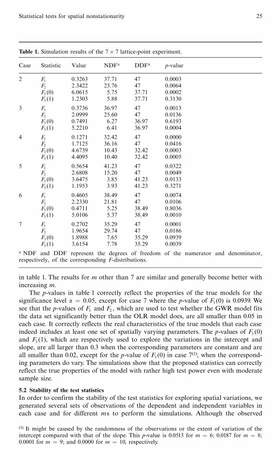
The p-values in table 1 correctly reflect the properties of the true models for thesignificance level a � 0:05, except for case 7 where the p-value of F3 (0) is 0.0939. Wesee that the p-values of F1 and F2 , which are used to test whether the GWR model fitsthe data set significantly better than the OLR model does, are all smaller than 0.05 ineach case. It correctly reflects the real characteristics of the true models that each caseindeed includes at least one set of spatially varying parameters. The p-values of F3 (0)and F3 (1), which are respectively used to explore the variations in the intercept andslope, are all larger than 0.3 when the corresponding parameters are constant and areall smaller than 0.02, except for the p-value of F3 (0) in case 7(1), when the correspond-ing parameters do vary. The simulations show that the proposed statistics can correctlyreflect the true properties of the model with rather high test power even with moderatesample size.

5.2 Stability of the test statisticsIn order to confirm the stability of the test statistics for exploring spatial variations, wegenerated several sets of observations of the dependent and independent variables ineach case and for different ms to perform the simulations. Although the observed

Table 1. Simulation results of the 7� 7 lattice-point experiment.

Case Statistic Value NDFa DDFa p-value

2 F1 0.3263 37.71 47 0.0003F2 2.3422 23.76 47 0.0064F3 (0) 6.0615 5.75 37.71 0.0002F3 (1) 1.2303 5.88 37.71 0.3130

3 F1 0.3736 36.97 47 0.0013F2 2.0999 25.60 47 0.0136F3 (0) 0.7491 6.27 36.97 0.6193F3 (1) 5.2210 6.41 36.97 0.0004

4 F1 0.1271 32.42 47 0.0000F2 1.7125 36.16 47 0.0416F3 (0) 4.6739 10.43 32.42 0.0003F3 (1) 4.4095 10.40 32.42 0.0005

5 F1 0.5654 41.23 47 0.0322F2 2.6808 15.20 47 0.0049F3 (0) 3.6475 3.85 41.23 0.0133F3 (1) 1.1953 3.93 41.23 0.3271

6 F1 0.4605 38.49 47 0.0074F2 2.2330 21.81 47 0.0106F3 (0) 0.4711 5.25 38.49 0.8036F3 (1) 5.0106 5.37 38.49 0.0010

7 F1 0.2702 35.29 47 0.0001F2 1.9654 29.74 47 0.0186F3 (0) 1.8988 7.65 35.29 0.0939F3 (1) 3.6154 7.78 35.29 0.0039

a NDF and DDF represent the degrees of freedom of the numerator and denominator,respectively, of the corresponding F-distributions.

(1) It might be caused by the randomness of the observations or the extent of variation of theintercept compared with that of the slope. This p-value is 0.0513 for m � 6; 0.0187 for m � 8;0.0001 for m � 9; and 0.0000 for m � 10, respectively.

Statistical tests for spatial nonstationarity 25

values of the test statistics, the degrees of freedom of the corresponding approximateddistributions, and the p-values vary from one set of observations to another, the resultsare all similar to those reported in table 1, and the difference between the p-values ofthe statistics corresponding to the varying parameters and nonvarying parameterssituations is large enough to support our claim that they correctly reflect the propertiesof the true models under some specified significance levels.

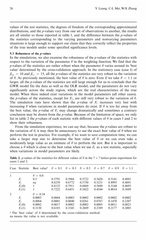
5.3 Robustness of the p-valuesIn the simulations, we also examine the robustness of the p-values of the statistics withrespect to the variation of the parameter y in the weighting function. We find that thep-values of the statistics are rather robust when the parameter y varies around its `bestvalue' determined by the cross-validation approach. In the stationary case (case 1) ofbi 0 � 10 and bi 1 � 15, all the p-values of the statistics are very robust to the variationof y. As previously mentioned, the best value of y is zero. Even if we take y � 1:1 orlarger, all the p-values of the statistics are still large enough for us to conclude that theGWR model fits the data as well as the OLR model, and the parameters do not varysignificantly across the study region, which are the real characteristics of the truemodel. When there indeed exist variations in the model parameters (all other cases),the p-values of the statistics, except for F2 , are still very robust to the variation of y.The simulation runs have shown that the p-value of F2 increases very fast withincreasing y when variations in model parameters do exist. If y is too far away fromthe best value, the p-value of F2 may change dramatically and sometimes a contraryconclusion may be drawn from the p-value. Because of the limitation of space, we onlylist in table 2 the p-values of each statistic with different values of y in cases 1 and 2 toshow their robustness.

From the simulation experience, we can say that, because the p-values are robust tothe variation of y, it may then be unnecessary to use the exact best value of y when weperform the test in practice. For example, if we want to save computation time, we cantake a larger step size to determine the best value of y or we can even take amoderately large value as an estimate of y to perform the test. But it is important tochoose a y which is close to the best value when we use F2 as a test statistic, especiallywhen variations in model parameters are likely.

Table 2. p-values of the statistics for different values of y in the 7� 7 lattice-point experiment forcases 1 and 2.

Case Statistic Best valuea y � 0:1 y � 0:3 y � 0:5 y � 0:7 y � 0:9 y � 1:1

1 y � 0:0F1 0.5 0.5791 0.5968 0.5722 0.5420 0.5141 0.4881F2 na 0.8239 0.6772 0.5750 0.5231 0.4995 0.4891F3 (0) 1 0.8125 0.7911 0.6869 0.5849 0.5144 0.4695F3 (1) 1 0.7222 0.6451 0.5422 0.4544 0.4014 0.3689

2 y � 0:34F1 0.0003 0.0064 0.0003 0.0002 0.0002 0.0002 0.0002F2 0.0064 0.0001 0.0040 0.0261 0.0767 0.1470 0.2207F3 (0) 0.0002 0.0017 0.0002 0.0002 0.0005 0.0011 0.0021F3 (1) 0.3130 0.6185 0.3345 0.2689 0.2389 0.2177 0.2003

a The `best value' of y determined by the cross-validation method.na means the value is not available.

26 Y Leung, C-L Mei,W-X Zhang

6 PredictionAlthough the GWR technique is used mainly for exploring spatial nonstationarity ofthe parameters, prediction is still an important aspect in regression analysis. For theGWR model, solution of the prediction problem is straightforward. In this section, theprediction method based on the GWR model is discussed and an approximatedconfidence interval for the true value of the dependent variable at a new location isestablished.

If a GWR model can describe a given data set well, we can use it to predict the truevalue of the dependent variable given the observations of the independent variables ata new point in the study area. Let (x01 x02 .:: x0p ) be an observation of the independentvariables at new location p0 and xT

0 � (1 x01 x02 .:: x0p ). Then the predicted value fory0 (the true value of the dependent variable at p0 ) is

y0 � xT0 b� p0 � , (69)

where

b� p0 � � �XTW� p0 �X�ÿ1XTW� p0 �Y , (70)

and W( p0 ) is known at this moment because the parameter in it has been determinedin the model calibration process and the distances from p0 to other points where thedata are observed are also known once the point p0 is given.

The next stage is to construct a confidence interval for y0 . As pointed out pre-viously, a local fitting technique tends to find a low-bias estimate.We assume that y0 isan unbiased estimator of E( y0 ), that is,

E� y0 � � E� y0 � . (71)

We know from equation (69) and (70) that y0 is not related to y0. Therefore, y0 and y0are independent and we have

var�y0 ÿ y0 � � var� y0 � � var� y0 �� varfxT

0 �XTW� p0 �X�ÿ1XTW� p0 �Y g � s 2

� xT0 �XTW� p0 �X�ÿ1XTW� p0 �var�Y �W� p0 �X�XTW� p0 �X�ÿ1x0 � s 2

� f1� xT0 �XTW� p0 �X�ÿ1XTW2� p0 �X�XTW� p0 �X�ÿ1x0gs 2 . (72)

For simplicity, let

S� p0 � � xT0 �XTW� p0 �X�ÿ1XTW2� p0 �X�XTW� p0 �X�ÿ1x0 . (73)

Under the assumption made in equation (71) and the fact that y0 and y0 are normallydistributed, we obtain

y0 ÿ y0

s�1� S� p0 ��1=2� N�0, 1� . (74)

Also, from section 3.1 we know that the distribution of the statistic d 21 s

2=d2s2 can be

approximated by a w 2 distribution with d 21=d2 degrees of freedom. So, the distribution

of the statistic

T � y0 ÿ y0

s�1� S� p0 ��1=2(75)

can be approximated by a t-distribution with d 21=d2 degrees of freedom, where s 2

is defined by equation (21). Given a confidence level a, we write ta2(d 2

1=d2 � as the

Statistical tests for spatial nonstationarity 27

upper 100( a2) percentage point. Thus an approximated confidence interval of y0 with

confidence 1ÿ a is obtained as follows:

y0 � s�1� S� p0 ��1=2ta2

�d 21

d2

�. (76)

7 ConclusionThe GWR model appears to be a useful means to explore variation of the slope betweenthe dependent variable and the independent variables over space. To fill the theoreticalgap in the literature, we have proposed in this paper some statistical testing methods bywhich the goodness of fit of the GWR model can be evaluated in comparison with theOLR model, and the variation of the parameters over space can be determined.We havealso formulated a procedure for choosing significant independent variables from a largenumber of candidate independent variables for the model. Based on the theoreticalresults, we further investigated the prediction issue of the GWR model and constructedan approximate confidence interval of the true value of the dependent variable.

Because of the complexity of parameter estimation in the GWR model, it seems tobe a difficult task to find the exact distributions of the proposed statistics. Also, if wetake account of the fact that the parameter in the weighting function is determined bythe cross-validation approach and is, therefore, related to the observations, this willmake it more difficult to find the exact distributions of the testing statistics. So, from apractical point of view, finding approximated distributions is a feasible way to solvethis kind of problem. We have thus chosen one simple but accurate method to approx-imate the distribution of the quadratic form with normal variables and positive semi-definite matrix, and the distributions of the other proposed statistics. The simplicity incomputation is apparent. The simulation results have shown that the test power of theproposed statistics is rather high and their p-values are rather robust to the variation ofthe parameter in the weighting matrix. Nevertheless, more simulations with certainstructures in the x-variables still need to be performed in further studies in order tounderstand the generality of the proposed approximation methods in more complexenvironments. Furthermore, although the proposed approximations are sensible, it isalso worthwhile carrying out further research to find the exact distributions of theproposed test statistics. Based on the exact distribution theory of quadratic forms innormal variables (for example, see Imhof, 1961) which has recently been used in the testfor spatial autocorrelation (Tiefelsdorf and Boots, 1995; Hepple, 1998), it might bepossible to use this line of thinking to derive the exact p-values for the proposedstatistics in this paper. If this possibility can be confirmed, it could then provide auseful way of checking the validity of our approximation methods. However, it isobvious that the computation overhead will be considerable.

Although some further studies are still needed on this topic, with the presenttheoretical investigation, not only does the GWR model allow complex spatial varia-tions in parameters to be identified, mapped, and modeled, but we can also make itpossible to perform the significance test in a conventional statistical manner.

Acknowledgement. This project is supported by the earmarked grant CUHK 4037/97H of theHong Kong Research Grants Council.

ReferencesAnselin L, 1988 Spatial Econometrics: Methods and Models (Kluwer Academic, Dordrecht)Anselin L,1990,` Spatial dependence and spatial structural instability in applied regression analysis''

Journal of Regional Science 30 185 ^ 207Bowman AW, 1984, `An alternative method of cross-validation for the smoothing of density

estimate'' Biometrika 71 353 ^ 360

28 Y Leung, C-L Mei,W-X Zhang

Brunsdon C F, 1995, ` Estimating probability surfaces for geographical point data: an adaptivekernel algorithm'' Computers and Geosciences 21 877 ^ 894

Brunsdon C, Fotheringham A S, CharltonM,1996, ` Geographically weighted regression: a methodfor exploring spatial nonstationarity'' Geographical Analysis 28 281 ^ 298

Brunsdon C, Fotheringham A S, Charlton M, 1997, ` Geographical instability in linear regressionmodellingöa preliminary investigation'', in New Techniques and Technologies for Statistics II(IOS Press, Amsterdam) pp 149 ^ 158

Casetti E, 1972, ` Generating models by the expansion method: applications to geographicalresearch'' Geographical Analysis 4 81 ^ 91

Casetti E, 1982, ` Drift analysis of regression analysis: an application to the investigation of fertilitydevelopment relations''Modeling and Simulation 13 961 ^ 966

Casetti E, 1986, ` The dual expansion method: an application for evaluating the effects of populationgrowth on development'' IEEE Transactions on Systems, Man and Cybernetics 16 29 ^ 39

CharltonM, FotheringhamAS, BrunsdonC,1997,` The geographyof relationships: an investigationof spatial non-stationarity'', inSpatialAnalysisofBiodemographicDataEds J-P Bocquet-Appel,D Courgeau, D Pumain (John Libbey Eurotext, Montrouge) pp 23 ^ 47

Cleveland W S, 1979, ` Robust locally weighted regression and smoothing scatter-plots'' Journalof the American Statistical Association 74 829 ^ 836

ClevelandWS, Devlin S J, 1988,``Locally weighted regression: an approach to regression analysis bylocal fitting'' Journal of the American Statistical Association 83 596 ^ 610

Cleveland W S, Devlin S J, Grosse E, 1988, ` Regression by local fitting: methods, properties andcomputational algorithms'' Journal of Econometrics 37 87 ^ 114

Dobson A J, 1990 An Introduction to Generalized Linear Models (Chapman and Hall, London)Foster S A, Gorr W L, 1986, `An adaptive filter for estimating spatially-varying parameters:

application to modelling police hours spent in response to calls for service''ManagementScience 32 878 ^ 889

Fotheringham A S, 1997, ` Trends in quantitative methods I: stressing the local'' Progress inHuman Geography 21 88 ^ 96

Fotheringham A S, Pitts T C, 1995, ` Directional variation in distance-decay'' Environment andPlanning A 27 715 ^ 729

Fotheringham A S, Charlton M, Brunsdon C, 1996, ` The geography of parameter space: aninvestigation into spatial non-stationarity'' International Journal of Geographical InformationSystems 10 605 ^ 627

Fotheringham A S, Charlton M, Brunsdon C, 1997a, ` Measuring spatial variations in relationshipswith geographically weighted regression'', in Recent Developments in Spatial AnalysisEds M M Fischer, A Getis (Springer, London) pp 60 ^ 82

Fotheringham A S, Charlton M, Brunsdon C, 1997b, ` Two techniques for exploring non-stationarity in geographical data'' Geographical Systems 4 59 ^ 82

Gorr W L, Olligschlaeger A M, 1994, ``Weighted spatial adaptive filtering: Monte Carlo studiesand application to illicit drug market modelling'' Geographical Analysis 26 67 ^ 87

Hepple LW, 1998, ` Exact testing for spatial autocorrelation among regression residuals''Environment and Planning A 30 85 ^ 109

Hocking R R, 1996 Methods and Applications of Linear Models (JohnWiley, NewYork)Imhof J P, 1961, ` Computing the distribution of quadratic forms in normal variables''Biometrika 48

419 ^ 426Johnson N L, Kotz A B, 1970 Continuous Univariate Distributions (JohnWiley, NewYork)Jones J P, Casetti E, 1992 Applications of the Expansion Method (Routledge, London)Neter J,WassermanW, Kutner M H, 1989 Applied Linear Regression Models 2nd edition (Irwin,

Homewood, IL)Openshaw S, 1993, ` Exploratory space ^ time-attribute pattern analysis'', in Spatial Analysis and

GIS Eds A S Fotheringham, P A Rogerson (Taylor and Francis, London) pp 147 ^ 163SolomonH, StephensMA,1977,` Distribution of a sum ofweighted chi-square variables''Journal of

the American Statistical Association 72 881 ^ 885Solomon H, Stephens M A, 1978, `Approximations to density functions using Pearson curves''

Journal of the American Statistical Association 73 153 ^ 160Stuart A, Ord J K, 1994 Kendall's Advanced Theory of Statistics.Volume 1, Distribution Theory

6th edition (Edward Arnold, London)Tiefelsdorf M, Boots B, 1995, ` The exact distribution of Moran's I '' Environment and Planning A

27 985 ^ 999Wand M P, Jones M C, 1995 Kernel Smoothing (Chapman and Hall, London)

Statistical tests for spatial nonstationarity 29

APPENDIX AThe variance of RSSg=s

2

From equation (22),

RSSg

s 2��EEs

�T�Iÿ L�T�Iÿ L� EE

s, (A1)

where EE=s � N(0, I), and (Iÿ L)T(Iÿ L) is a real symmetric and positive semidefinitematrix. According to the theory of matrix algebra, there exists an orthogonal matrix Pof order n such that

PT�Iÿ L�T�Iÿ L�P � K � diag�l1, l2 , .:: , ln � , (A2)

where K is a diagonal matrix having the eigenvalues, l1, l2 , .:: , ln , of the matrix(Iÿ L)T(Iÿ L) in its main diagonal. Let

g � �Z1 Z2 .:: Zn �T � PT EEs. (A3)

According to the properties of multivariate normal distribution, Z1, Z2 , .:: , Zn areindependent identically distributed (iid) random variables with common distributionN(0, 1). On the other hand, under the orthogonal transformation (A3), we obtain

RSSg

s 2� gTPT�Iÿ L�T�Iÿ L�Pg

� gTKg

�Xni � 1

li Z2i . (A4)

It is well know that Z 2i (i � 1, 2, .:: , n) are iid random variables with common w 2

distribution with one degree of freedom. Therefore var(Z 2i ) � 2, and

var�RSSg

s 2

��Xni � 1

l 2i var�Z 2

i � � 2Xni � 1

l 2i . (A5)

We know from the theory of matrix algebra that l 21 , l

22 , .:: , l

2n are eigenvalues of the

matrix [(Iÿ L)T(Iÿ L)]2. Therefore

var�RSSg

s 2

�� 2 tr��Iÿ L�T�Iÿ L��2 � 2d2 . (A6)

30 Y Leung, C-L Mei,W-X Zhang

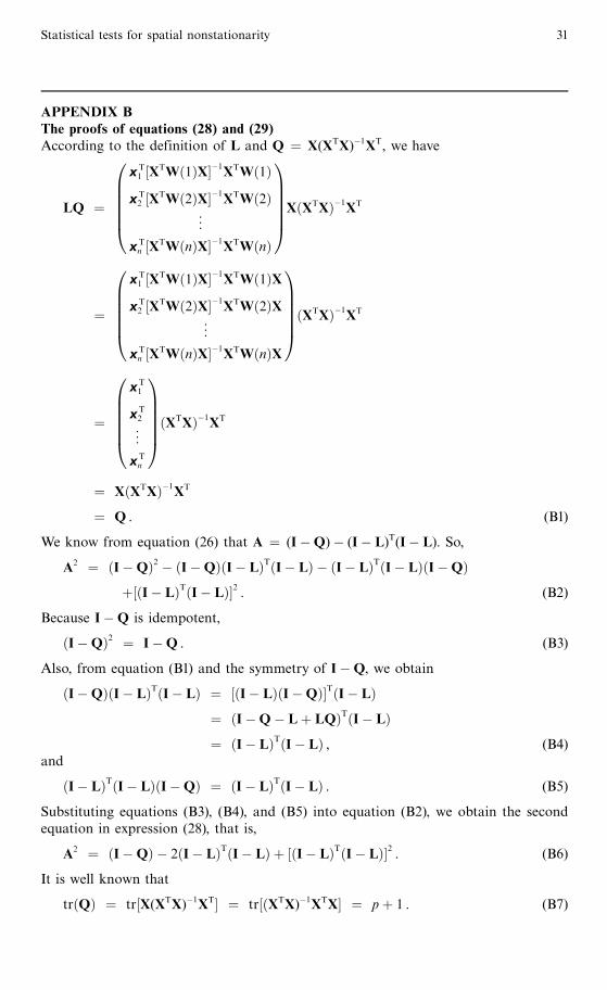
APPENDIX BThe proofs of equations (28) and (29)According to the definition of L and Q � X(XTX)ÿ1XT, we have

LQ �

xT1 �XTW�1�X�ÿ1XTW�1�

xT2 �XTW�2�X�ÿ1XTW�2�

..

.

xTn �XTW�n�X�ÿ1XTW�n�

0BBBBB@

1CCCCCAX�XTX�ÿ1XT

�

xT1 �XTW�1�X�ÿ1XTW�1�X

xT2 �XTW�2�X�ÿ1XTW�2�X

..

.

xTn �XTW�n�X�ÿ1XTW�n�X

0BBBBB@

1CCCCCA�XTX�ÿ1XT

�

xT1

xT2

..

.

xTn

0BBBBB@

1CCCCCA�XTX�ÿ1XT

� X�XTX�ÿ1XT

� Q . (B1)

We know from equation (26) that A � (IÿQ)ÿ (Iÿ L)T(Iÿ L). So,

A2 � �IÿQ�2 ÿ �IÿQ��Iÿ L�T�Iÿ L� ÿ �Iÿ L�T�Iÿ L��IÿQ����Iÿ L�T�Iÿ L��2 . (B2)

Because IÿQ is idempotent,

�IÿQ�2 � IÿQ . (B3)

Also, from equation (B1) and the symmetry of IÿQ, we obtain

�IÿQ��Iÿ L�T�Iÿ L� � ��Iÿ L��IÿQ��T�Iÿ L�� �IÿQÿ L� LQ�T�Iÿ L�� �Iÿ L�T�Iÿ L� , (B4)

and

�Iÿ L�T�Iÿ L��IÿQ� � �Iÿ L�T�Iÿ L� . (B5)

Substituting equations (B3), (B4), and (B5) into equation (B2), we obtain the secondequation in expression (28), that is,

A2 � �IÿQ� ÿ 2�Iÿ L�T�Iÿ L� � ��Iÿ L�T�Iÿ L��2 . (B6)

It is well known that

tr�Q� � tr�X(XTX)ÿ1XT� � tr��XTX)ÿ1XTX� � p� 1 . (B7)

Statistical tests for spatial nonstationarity 31

Therefore

tr�A� � tr��IÿQ� ÿ �Iÿ L�T�Iÿ L��� nÿ pÿ 1ÿ d1 ,

tr�A2 � � trf�IÿQ� ÿ 2�Iÿ L�T�Iÿ L� � ��Iÿ L�T�Iÿ L��2g� nÿ pÿ 1ÿ 2d1 � d2 ,

8>>>><>>>>: (B8)

where di � tr[(Iÿ L)T(Iÿ L)] i (i � 1, 2).

ß 2000 a Pion publication printed in Great Britain

32 Y Leung, C-L Mei,W-X Zhang

All in-text references underlined in blue are linked to publications on ResearchGate, letting you access and read them immediately.