Statistical reconstruction of two-phase random mediaengweb.swan.ac.uk/...CAS_Statistical_Reconstruction_of_Two-Phase_Random... · phase composite materials with random morphology,

Computers and Structures 137 (2014) 78–92

Contents lists available at SciVerse ScienceDirect

Computers and Structures

journal homepage: www.elsevier .com/locate/compstruc

Statistical reconstruction of two-phase random media

0045-7949/$ - see front matter � 2013 Elsevier Ltd. All rights reserved.http://dx.doi.org/10.1016/j.compstruc.2013.03.019

⇑ Corresponding author. Tel.: +44 (0) 1792 602256; fax: +44 (0) 1792 295676.E-mail address: [email protected] (C.F. Li).

J.W. Feng a, C.F. Li a,⇑, S. Cen b,c, D.R.J. Owen a

a Civil & Computational Engineering Centre, College of Engineering, Swansea University, United Kingdomb Department of Engineering Mechanics, School of Aerospace, Tsinghua University, Beijing, Chinac Key Laboratory of Applied Mechanics, School of Aerospace, Tsinghua University, Beijing, China

a r t i c l e i n f o a b s t r a c t

Article history:Received 20 July 2012Accepted 24 March 2013Available online 25 April 2013

Keywords:Composite materialRandom microstructureSample reconstructionNon-Gaussian fieldFFT

A robust and efficient algorithm is proposed to reconstruct two-phase composite materials with randommorphology, according to given samples or given statistical characteristics. The new method is based onnonlinear transformation of Gaussian random fields, where the correlation of the underlying Gaussianfield is determined explicitly rather than through iterative methods. The reconstructed media can meetthe binary-valued marginal probability distribution function and the two point correlation function of thereference media. The new method, whose main computation is completed using fast Fourier transform(FFT), is highly efficient and particularly suitable for reconstructing large size random media or a largenumber of samples. Its feasibility and performance are examined through a series of practical exampleswith comparisons to other state-of-the-art methods in random media reconstruction.

� 2013 Elsevier Ltd. All rights reserved.

1. Introduction IðxÞ ¼0; if the material at x is in black phase

�: ð1Þ

Multi-phase random media such as rocks, concrete, alloy andcomposite materials are ubiquitous in the natural environmentand engineering. Their mechanical, thermal and electrical etc.properties exhibit a strong random nature with discontinuitieson the interfaces between different phases. The responses of mul-ti-phase random media subjected to force, thermal or other type ofloading are often of great interest to engineers and researchers, andsuch responses should be analyzed in the sense of statistics due tothe inherent heterogeneity. At present, Monte Carlo methods re-main the most popular and versatile approach for simulating therandomness of multi-phase random media and estimating theirstochastic responses. The effectiveness of Monte Carlo methods re-lies largely on rapid reconstruction of large amounts of samplesthat can accurately represent the diversity and variation of thepractical random media under simulation.

The main focus of this work is on the reconstruction of two-phase composite materials with random morphology, based onstatistical characteristics derived from a few measured samples.The proposed reconstruction method is general and applicable toother types of random media as well, and instead of using the term‘‘composite’’, we will use the general term ‘‘random media’’ for theremainder of the paper.

For a two-phase (black & white) random medium D, the indicatorfunction I(x), "x 2 D is defined as

1; if the material at x is in white phase

Due to the random nature of phase distribution, the indicator func-tion is often treated in the context of probability as a binary valuedrandom field, denoted by I(x, x) where x indicates a basic randomevent.

In practice, the random field I(x, x) is often assumed to be sta-tionary (also termed as statistically homogeneous in [1–3]) up tothe second order, so that its mean l and variance r2 are invariantwhen shifted in space. In addition, the autocorrelation function be-tween points x and x + s depends only on the relative position s ofthe two points, i.e.

RIðsÞ ¼E½ðIðx;xÞ � lÞðIðxþ s;xÞ � lÞ�

r2 ; 8x; ð2Þ

where E() is the expectation operator. The range of RI(s) is �1 6RI(s) 6 1 (Schwarz inequality).

Another assumption of I(x, x) is ergodicity. That is, the ensem-ble average of statistical parameters can be derived by the spaceaverage of these parameters over a sufficiently large sample.

Given a few, or even only one, realizations of the random media,the task of reconstruction is to extract statistical parameters (l, r2

and RI(s) etc.) regarding the random field I(x, x) and generate sam-ples that obey the same statistics as the reference realizations.

2. Overview

2.1. Related work

Over the past few decades, random media reconstruction hasattracted growing attention from both academia and industry, in

http://crossmark.crossref.org/dialog/?doi=10.1016/j.compstruc.2013.03.019&domain=pdf

http://dx.doi.org/10.1016/j.compstruc.2013.03.019

mailto:[email protected]

http://dx.doi.org/10.1016/j.compstruc.2013.03.019

http://www.sciencedirect.com/science/journal/00457949

http://www.elsevier.com/locate/compstruc

J.W. Feng et al. / Computers and Structures 137 (2014) 78–92 79

particular in the fields of composite materials, geostatistics andcomputational mechanics. To date, there are four main categoriesof reconstruction methods: the random set method, the stochasticoptimization method, the maximum entropy method and the iter-ative nonlinear transformation method.

The random set method [4–6] is based on Boolean operations(union, intersection, dilation, erosion, et al. [7]) of random sets.This method is fast but it is limited to a few types of randommedia with relatively simple morphology, e.g. composites withsphere or polygon inclusions or Voronoi cell structure. For exam-ple, if the inclusion phase is spheres, their centers can be gener-ated following a Poisson distribution; the radius can be similarlyassumed to obey certain probability distribution; and adjacentspheres need to be trimmed if they overlap. However, for com-posites with complicated structures, e.g. amorphous phases, therandom set objects are difficult to locate and operate, leading todeterioration in efficiency. In short, the random set method is fastand effective for certain types of random media, but is not a uni-versal method.

Yeong and Torquato [1,8] introduced a simulated annealingmethod for generating digitalized random media realizations.Given a scanned image of the target random medium, this methodstarts from an initial configuration satisfying the volume fraction,and for the simulated image it successively performs randomexchanges of pixels with different colors to minimize certain‘‘energy’’ that measures the difference in correlation function,two-point cluster function [9] or n-point correlation function [10]etc. between the reference image and the simulated image. If theenergy decreases after the exchange, the new configuration is con-sidered superior to the old one, and the exchange is accepted. If theenergy increases after the exchange, the new configuration is con-sidered possible to be a transitional state from ‘‘local optimum’’ to‘‘global optimum’’, and hence the exchange is accepted with aprobability, which depends on the energy of the old and the newconfigurations and the annealing temperature [1]. Recently, sev-eral other stochastic optimization approaches were developed toovercome the low efficiency of the simulated annealing method,including genetic algorithm, Tabu-list and hybrid optimizationmethods [3,11]. The stochastic optimization method is perhapsthe most flexible method for reconstructing random media sam-ples, and it allows a wide range of statistical characteristics to beincorporated in sample generation. Its disadvantage is the expen-sive computational burden when large samples (either in size orin number) are required.

In the maximum entropy method [10,12,13], random media aremodeled as Markov random fields. The joint probability distribu-tion of Markov random fields is the Gibbs distribution [14], whichis exactly the probability distribution that maximizes the entropyunder expectation-type confinements (e.g. l, r2, RI(s), etc)[15,16]. The explicit formation of the Gibbs distribution cannot beobtained because it is an infinite dimensional function. Thus, Mar-kov chain Monte Carlo (MCMC) methods [17] are employed to sam-ple from the Gibbs distribution, for which the Metropolis–Hastingsalgorithm [18,19] (a random walk MCMC method) has been a pop-ular choice. Similar to the stochastic optimization method, whichcan be viewed as a special type of the Metropolis–Hastings algo-rithm [19,20], a large number of random walk steps are oftenrequired to achieve the equilibrium distribution status of theMarkov chain. For practical use, the maximum entropy method iscriticized to be even slower than the stochastic optimization meth-od, and not suitable for large size problems [3].

The nonlinear transformation of Gaussian fields has been exten-sively used in modeling multivariate distributions [21,22]. Themarginal distribution of the non-Gaussian field is met exactly,

and the covariance of the underlying Gaussian field is computednumerically to satisfy the two point covariance requirement ofthe non-Gaussian field. This approach has been employed to modeltwo-phase random media [2,23,24]. However, the relationship be-tween the covariance of the non-Gaussian field and that of theGaussian field is ignored in [23,24], while using an iterative algo-rithm the covariance function of the underlying Gaussian field iscalculated in [2]. The most costly part of the nonlinear transforma-tion approach is to determine the nonnegative definite covariancefunction (nonnegative definite covariance matrix in the discretecase) of the underlying Gaussian field. In most of the literature[2] and [25–28], the Gaussian field is constructed from an initialpower spectral density (PSD) structure and an iterative algorithmis adopted to repeatedly update the PSD of the Gaussian field in or-der to make the PSD of the non-Gaussian field meet the target, andthis can be a very slow process for practical problems. Another lim-itation of this method is that the marginal distribution and thecovariance of the non-Gaussian field need to satisfy a compatibilityrelation in advance [29].

In this paper, the relationship between the correlation of thebinary field and that of the Gaussian field is derived explicitly toavoid the costly iteration procedure commonly employed in exist-ing nonlinear transformation approaches. The compatibility rela-tion between the marginal distribution and the autocorrelation ofbinary valued fields are also rigorously investigated, and provedto be not a critical restriction. These new developments signifi-cantly improve the efficiency of sample generation, allowing thou-sands of large samples to be generated within a few minutes. Themain limitation of the method is that it does not utilize other sta-tistical characteristics (e.g. n-point correlation and lineal-pathfunction). However, numerical examples demonstrate that thenew method is suitable for a variety of types of two-phase randommedia, as two-point correlation contains considerable informationon random morphology.

2.2. Preliminary knowledge: spectral decomposition of stationaryrandom fields

The Wiener–Khinchin theorem [30,31] states that the PSD f(X)of a stationary second-order random field a(x, x) is the Fouriertransform of the corresponding autocorrelation function R(s). Ifa(x, x) is a periodical stochastic process [32,33] with a period of2N, i.e. aðx1; . . . ; xn;xÞ ¼ aðx1 þ 2N1; . . . ; xn þ 2Nn;xÞ, the discreteversion of the Wiener–Khinchin theorem can be written as [34,35]:

f ðX1; . . . XnÞ ¼XN1

s1¼�N1þ1

. . .XNn

sn¼�Nnþ1

Rðs1; . . . ; snÞe�Xn

j¼1

piNj

Xjsj

;

Xj ¼ ½�Nj þ 1;Nj� ð3Þ

Rðs1; � � � ; snÞ ¼1Q

jð2NjÞXN1

X1¼�N1þ1

� � �XNn

Xn¼�Nnþ1

f ðX1; � � �XnÞe

Xn

j¼1

piNj

Xjsj

;

sj ¼ ½�Nj þ 1;Nj� ð4Þ

where i is the imaginary unit, Nj are positive integers, the integercoordinates s1; . . . ; sn denote the space domain, the integer coordi-nates X1; . . . Xn denote the frequency domain, and f ðX1; . . . XnÞ is realand nonnegative valued due to the nonnegative definite property ofRðs1; . . . ; snÞ.

Then, a(x, x) can be represented by an orthogonal incrementprocess:

80 J.W. Feng et al. / Computers and Structures 137 (2014) 78–92

aðx1; . .. ;xn;xÞ¼Eðaðx1; . .. ;xn;xÞÞ

þ 1Qnj¼1ð2NjÞ

XN1

X1¼�N1þ1

. . .XNn

Xn¼�Nnþ1

nðX1;. . .Xn;xÞe

Xn

j¼1

piNj

Xjxj

;

xj¼½�Njþ1;Nj� ð5Þ

where nðX1; . . . Xn;xÞ are uncorrelated, complex valued randomvariables satisfying

EðnðXa1; . . . Xan;xÞÞ ¼ 0 8Xaj 2 Z½�Nj þ 1;Nj� ð6Þ

and

EðnðXa1;. . .Xan;xÞnðXb1; .. .Xbn;xÞÞ

¼Yn

j¼1

ð2NjÞf ðXa1; � ��XanÞr2 if Xaj¼Xbj;8j

0 else

8><>: 8Xaj;Xbj 2Z½�Njþ1;Nj�:

ð7Þ

Especially, if aðx1; . . . ; xn;xÞ is a Gaussian random field, thennðX1; . . . Xn;xÞ are all independent complex Gaussian randomvariables.

The Wiener–Khinchin theorem, which is a second order statisti-cal decomposition method, plays an important role in the analysisof stationary Gaussian fields as Gaussian fields are completelydetermined by their first two statistical moments. However, fornon-Gaussian random fields, it is difficult to directly generate sam-ples because the uncorrelated random variables nðX1; . . . Xn;xÞ arenot independent and their joint probability distribution is un-known a priori.

3. Nonlinear transformation of Gaussian fields

Let G(x, x) be a stationary Gaussian field with zero mean andunit variance, and let RG(s) denote its autocorrelation function.The Gaussian field G(x, x) is uniquely determined by RG(s). Themarginal distribution of G(x, x) can be expressed as

FGðyÞ ¼12

1þ erfyffiffiffi2p� ��

ð8Þ

where erf() denotes the error function.To reconstruct the two-phase random medium defined by I(x,

x) in Eq. (1), we aim to find a transformation of G(x, x) such thatRG(s) can be explicitly specified to give the transformed Gaussianfield the same mean, variance, covariance (or autocorrelation)and marginal distribution as I(x, x). Let p0 denote the volume frac-tion of the black phase. It is then trivial to obtain the mean and var-iance of I(x, x) as

l ¼ 1� p0; ð9Þ

r2 ¼ p0ð1� p0Þ: ð10Þ

Define a transformation function T(y) as

TðyÞ ¼0 if y 6 F�1

G ðp0Þ1 if y > F�1

G ðp0Þ

(ð11Þ

where F�1G ðp0Þ is the separation point at which the distribution func-

tion FG(y) takes the value of p0. Let

I�ðx;xÞ ¼ TðGðx;xÞÞ: ð12Þ

It is easy to verify that the transformed random field I⁄(x, x) is sta-tionary and has the same marginal distribution, mean and varianceas I(x, x). The next step is to determine RG(s) so that I⁄(x, x) followsthe same autocorrelation RI(s). Once RG(s) is determined, it isstraightforward to generate samples of G(x, x) following theWiener–Khinchin theorem (3)–(7), which can be further trans-formed to produce samples of I(x, x) .

3.1. The relationship between autocorrelations RG(s) and RI(s)

For any two points x1 and x2 = x1 + s in the medium, the auto-correlation function of the transformed two-phase random med-ium I⁄(x, x) can be computed by substituting Eq. (12) into Eq.(2), i.e.

R�I ðsÞ ¼E½ðTðGðx1;xÞÞ � lÞðTðGðx2;xÞÞ � lÞ�

r2

¼Z þ1

�1

Z þ1

�1

ðTðy1Þ � lÞðTðy2Þ � lÞr2 fg2ðy1; y2;RGðsÞÞdy1dy2

ð13Þ

where

fg2ðy1; y2;RGðsÞÞ ¼1

2pffiffiffiffiffiffiffiffiffiffiffiffiffiffiffiffiffiffiffiffiffiffiffi1� RGðsÞ2

q

� exp�1

2ð1� RGðsÞ2Þðy2

1 þ y22 � 2RGðsÞy1y2Þ

!

ð14Þ

is the joint probability density function (PDF) of a standard bivariateGaussian distribution with zero mean, unit variance and autocorre-lation RGðsÞ .

Following Eq. (11), the integrand ðTðy1Þ�lÞðTðy2Þ�lÞr2 in Eq. (13) can be

computed as

ðTðy1Þ � lÞðTðy2Þ � lÞr2

¼

ð1� p0Þ=p0 if y1 2 �1; F�1G ðp0Þ

i�; y2 2 ð�1; F�1

G ðp0ÞÞ

�1 if y1 2 �1; F�1G ðp0Þ

i�; y2 2 ðF

�1G ðp0Þ;1Þ

�1 if y1 2 ðF�1G ðp0Þ;1Þ; y2 2 �1; F�1

G ðp0Þi�

p0=ð1� p0Þ if y1 2 ðF�1G ðp0Þ;1Þ; y2 2 ðF�1

G ðp0Þ;1Þ

8>>>>>>><>>>>>>>:

:ð15Þ

Substituting Eqs. (15) into (13) yields

R�I ðsÞ ¼ �1þ 1p0

Z F�1G ðp0Þ

�1

Z F�1G ðp0Þ

�1fg2ðy1; y2;RGðsÞÞdy1dy2

þ 11� p0

Z þ1

F�1G ðp0Þ

Z þ1

F�1G ðp0Þ

fg2ðy1; y2;RGðsÞÞdy1dy2: ð16Þ

Due to the symmetry of fg2ðy1; y2;RGðsÞÞ (14), i.e. fg2ðy1; y2;RGðsÞÞ ¼fg2ð�y1;�y2;RGðsÞÞ, the autocorrelation R�I ðsÞ can be further simpli-fied into

R�I ðsÞ ¼ �1þ 1p0

Z F�1G ðp0Þ

�1

Z F�1G ðp0Þ


þ 11� p0

Z �F�1G ðp0Þ

�1

Z �F�1G ðp0Þ


¼ �1þ 1p0

Fg2ðF�1G ðp0Þ; F�1

G ðp0Þ;RGðsÞÞ

þ 11� p0

Fg2ð�F�1G ðp0Þ;�F�1

G ðp0Þ;RGðsÞÞ ð17Þ

where

Fg2ðy1; y2;RGðsÞÞ ¼Z y1

�1

Z y1

�1fg2ðz1; z2;RGðsÞÞdz1dz2 ð18Þ

is the cumulative distribution function corresponding to the PDFfg2(y1, y2, RG(s)).

In Eq. (17), the relationship between R�I ðsÞ and RG(s) depends onthe volume fraction p0. Due to the symmetry of the PDF fg2(y1, y2,RG(s)), it is straightforward to prove that


R�I ðs;p0Þ ¼ R�I ðs;1� p0Þ: ð19Þ

For a fixed volume fraction p0, Eq. (17) explicitly expressesR�I ðsÞ, the autocorrelation of the transformed two-phase randommedia, as a nonlinear function of RG(s), the autocorrelation of theunderlying Gaussian random field. Given the value of R�I ðsÞ, thecorresponding RG(s) can be solved, at least in principle, throughan iterative solver. It is proved in the following section that R�I ðsÞis monotonic with respect to RG(s). Hence, the solution of RG(s)can be significantly simplified through precomputation.

3.2. Compatibility relation between marginal distribution andautocorrelation

Following Eq. (17), the derivative of R�I ðsÞ with respect to RG(s)can be expressed as

−1 −0.5 0 0.5 1−1

−0.5

0

0.5

1

Fig. 1. Precomputed R�I ðsÞ � RGðsÞ curves.

Fig. 2. Comparison 1, image size 400 � 400 pixels. (a) The reference random media sampmethod in [1]; (c) a random media sample directly generated by our simulated annealingreconstructed by the iterative nonlinear transformation method; (f) a random media sa

dR�I ðsÞdRGðsÞ

¼ 1p0

Z F�1G ðp0Þ

�1

Z F�1G ðp0Þ

�1

dfg2ðy1; y2;RGðsÞÞdRGðsÞ

dy1dy2

þ 11� p0

Z �F�1G ðp0Þ

�1

Z �F�1G ðp0Þ

�1


dy1dy2 ð20Þ

where


¼ �RGðsÞðy21 þ y2

2Þ þ ðRGðsÞ2 þ 1Þy1y2 þ RGðsÞð1� RGðsÞ2Þð1� RGðsÞ2Þ2

� fg2ðy1; y2;RGðsÞÞ: ð21Þ

It can be computed that

Z z

�1

Z z

�1

dfg2ðy1;y2;RGðsÞÞdRGðsÞ

dy1dy2 ¼exp � z2

1þRGðsÞ

� 2p

ffiffiffiffiffiffiffiffiffiffiffiffiffiffiffiffiffiffiffiffiffiffi1�RGðsÞ2

q 8z2 ½�1;þ1�:

ð22ÞThus, the derivative (20) can be simplified as

dR�I ðsÞdRGðsÞ

¼ 1p0þ 1

1� p0

� � exp � ðF�1G ðp0ÞÞ2

1þRGðsÞ

� 2p

ffiffiffiffiffiffiffiffiffiffiffiffiffiffiffiffiffiffiffiffiffiffiffi1� RGðsÞ2

q � 0: ð23Þ

Eq. (23) implies that R�I ðsÞ is monotonically increasing with respectto RG(s). Hence, the range of R�I ðsÞ can be determined as:

maxðR�I ðsÞÞ ¼ limRGðsÞ!1

Z þ1

�1

Z þ1

�1


� fg2ðy1; y2;RGðsÞÞdy1dy2 ¼ 1; ð24Þ

minðR�I ðsÞÞ ¼ limRGðsÞ!�1

Z þ1

�1

Z þ1

�1


� fg2ðy1; y2;RGðsÞÞdy1dy2 ¼ �minðp0;1� p0Þmaxðp0;1� p0Þ

: ð25Þ

le from [1]; (b) the random media sample reconstructed by the simulated annealingcode; (d) the final sample after median filtering of (c); (e) a random media sample

mple reconstructed by the proposed method.


The above equations set the upper and lower limits of the autocor-relation R�I ðsÞ, which depend on the volume fraction p0. They form anecessary condition for reconstructing the target random mediumthrough the proposed nonlinear transformation of the Gaussianfield. That is, a two-phase random medium with volume fractionp0 and autocorrelation RI(s) can be reconstructed only if

RIðsÞ 2 � minðp0 ;1�p0Þmaxðp0 ;1�p0Þ

;1h i

. Note that, for practical random media with

irregular structures, the autocorrelation functions are almost al-ways above zero [9]. Hence, conditions (24)–(25) do not form a seri-ous restriction for the proposed method.

Fig. 3. Comparison 2, image size 400 � 400 pixels. (a) The reference random media sampmethod in [1]; (c) a random media sample directly generated by our simulated annealinreconstructed by the iterative nonlinear transformation method; (f) a random media sa

(a)

0 20 40 60 80 100−0.2

0

0.2

0.4

0.6

0.8

comparison1

the reference sample

simulated annealing method

iterative nonlinear transformation method

the proposed method

Fig. 4. Autocorrelation functions of the samples in the first comparison. (a) The autocorrela

3.3. Computational issues

Given the autocorrelation RI(s) of the target two-phase randommedium, to solve the autocorrelation RG(s) of the underlyingGaussian random field from the nonlinear Eq. (17) is potentiallytime consuming, if an iterative solver has to be adopted. Notingthat the relationship between R�I ðsÞ and RG(s) is monotonic, onecan precompute the function curve between R�I ðsÞ and RG(s) to savethe costly procedure of solving nonlinear equations. An example isshown in Fig. 1, where according to Eq. (17), the RGðsÞ ! R�I ðsÞcurves are computed for five volume fractions p0 ¼ 0:1;

le from [1]; (b) the random media sample reconstructed by the simulated annealingg code; (d) the final sample after median filtering of (c); (e) a random media samplemple reconstructed by the proposed method.

(b)

0 20 40 60 80 100−0.2

0

0.2

0.4

0.6

0.8

comparison1




the proposed method

tion along the horizontal direction; (b) the autocorrelation along the vertical direction.

(b)(a)

0 20 40 60 80 100−0.2

0

0.2

0.4

0.6

0.8

comparison2




the proposed method

0 20 40 60 80 100−0.2

0

0.2

0.4

0.6

0.8

comparison2




the proposed method

Fig. 5. Autocorrelation functions of the samples in the second comparison. (a) The autocorrelation along the horizontal direction; (b) the autocorrelation along the vertical direction.

0 1 2 3 4 5

x 104

0.4

0.6

0.8

1

Iteration Number

comparison1

0 1 2 3 4 5

x 104

0

0.5

1

Iteration Number

comparison2

Fig. 6. Convergence curves of the simulated annealing method.

0 5 10 15 200.2

0.3

0.4

0.5

Iteration Number

comparison1

0 5 10 15 200

0.2

0.4

Iteration Number

comparison2

Fig. 7. Convergence curves of the iterative nonlinear transformation method.


0:2; . . . ;0:5. Due to the symmetry relation in Eq. (19), theRGðsÞ ! R�I ðsÞ curves for p0 ¼ 0:6;0:7; . . . ;0:9 are symmetric. Thus,given the volume fraction p0 and the target autocorrelation RI(s),the corresponding autocorrelation RG(s) for the underlying Gauss-ian field can be readily obtained from these precomputed curvesthrough interpolation. Doing so avoids the expensive solution pro-cedure of the nonlinear RGðsÞ ! R�I ðsÞ equation, and can signifi-cantly accelerate sample reconstruction.

In the discrete case, function RG(s) can be expressed as a covari-ance matrix with unit diagonal entries and the absolute values ofoff diagonal entries less than one. Due to numerical approximation,the resulting matrix RG(s) may contain a few small negative eigen-values, violating the nonnegative definite requirement for a covari-ance matrix. Hence, a ‘‘nearest correlation matrix’’ [36–38] shouldbe constructed, which is a common practice for multivariate anal-ysis. To do this, we compute the PSD of RG(s) (see Eq. (3)) and setthe negative PSD entries to zero, after which the truncated PSD istransformed back following Eq. (4) to form a nonnegative definitecovariance matrix, ready for use on the Gaussian field.

4. Summary of the algorithm

The algorithm framework of the proposed sample generationmethod is summarized below.

Given a reference sample I(x, x), count the volume fraction p0

and estimate its autocorrelation function RI(s) through FFT(fast Fourier transform) of the sample spectrum. This is astandard practice of random signal processing, for whichdetailed description can be found in [39,40] and [41]. Note:the random medium is assumed with a 2N periodicboundary as shown in Eqs. (3) and (4). The period 2N islarger than the size of the random medium and selected asa power of 2 to enhance the efficiency of FFT, thus paddingwith 0 is required [39,40].

For the measured volume fraction p0, plot the R�I ðsÞ � RGðsÞcurve according to Eq. (17). The result is monotonic andexample curves are shown in Fig. 1.

Construct the covariance matrix of the underlying Gaussianfield, by registering the R�I ðsÞ � RGðsÞ curve with themeasured autocorrelation RI(s) of the target two-phaserandom medium.

Generate Gaussian field samples G(x, x), by using the spectraldecomposition method (3)–(7). This step is performed withFFT.

Generate samples of I(x, x) through the nonlineartransformation (11).

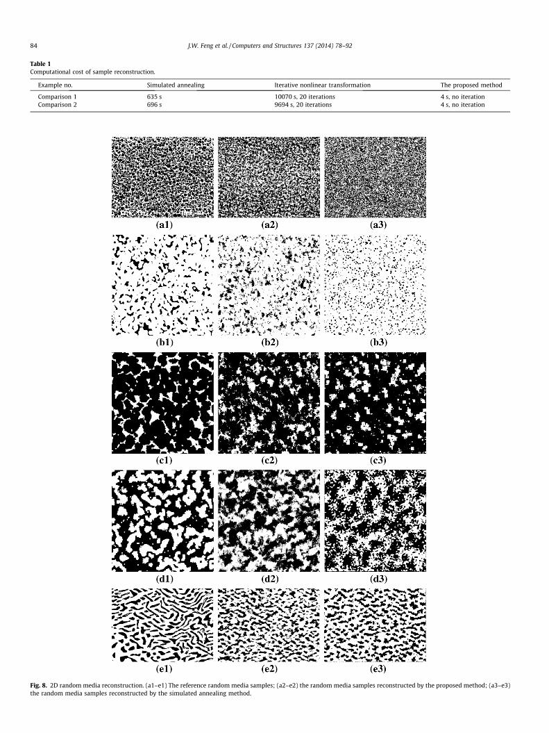
Fig. 8. 2D random media reconstruction. (a1–e1) The reference random media samples; (a2–e2) the random media samples reconstructed by the proposed method; (a3–e3)the random media samples reconstructed by the simulated annealing method.

Table 1Computational cost of sample reconstruction.

Example no. Simulated annealing Iterative nonlinear transformation The proposed method

Comparison 1 635 s 10070 s, 20 iterations 4 s, no iterationComparison 2 696 s 9694 s, 20 iterations 4 s, no iteration



The main computational cost of the proposed algorithm is the
FFT operation involved in step 4, whose computational complexityis log L proportional to the reconstructed sample size L. This highcomputational efficiency allows large sample sets (in terms of bothsample size and sample number) to be reconstructed on a commod-ity computer with moderate cost. The efficiency and accuracy of theproposed method are demonstrated by a number of examples in thenext section with comparisons to other state-of-the-art methods.
A free MATLAB� code of the proposed method is available uponrequest.

5. Examples

A number of examples are presented in this section to demon-strate the performance of the proposed method. First, the newmethod is compared with other state-of-the-art methods in the lit-erature, including the simulated annealing method [1] and the iter-ative nonlinear transformation method [26,28]. The random setmethod [4–6] and the maximum entropy method [10,12,13] arenot chosen for comparison, because the former is limited to afew special geometries, and the latter has high computational

(a

(b

0 10 20 30 40 50

0

0.2

0.4

0.6

0.8

1

2D random medium a

a1,the reference sample

a2,the proposed method

a3,simulated annealing method

0 10 20 30 40 50

0

0.2

0.4

0.6

0.8

1

2D random medium b

b1,the reference sample

b2,the proposed method

b3,simulated annealing method

Fig. 9. Autocorrelation functions of the 2D random media samples in Fig. 8. Left: the auvertical direction.

and implementation complexity. After the comparison, the newmethod is applied to a wide range of different random media todemonstrate its accuracy and applicability. Finally, large-scale 3Dcases are considered, and the new method is used to reconstruct3D samples for nuclear graphite Gilsocarbon measured fromthree-dimensional X-ray scanning.

All examples are simulated on a PC with an Intel Core i73.40 GHz processor and 16 GB memory.

5.1. Comparison

To help examine the performance of the proposed method, wehave also implemented the simulated annealing method [1] andthe iterative nonlinear transformation method [26,28]. For com-parison, we took two random media samples from [1], and recon-structed the associated samples using three different methods.Shown in Fig. 2(a) and (b) are a random media example and areconstructed sample taken from [1]. Fig. 2(c) and (d) is a samplereconstructed using our own implementation of the simulatedannealing method and for fair comparison, we adopted the samealgorithmic parameters as [1]. As the pixel exchanges are operatedon disks with a diameter of 17 pixels, the direct reconstruction

)

)

0 10 20 30 40 50

0

0.2

0.4

0.6

0.8

1

2D random medium a



a3,simulated annealing method

0 10 20 30 40 50

0

0.2

0.4

0.6

0.8

1

2D random medium b



b3,simulated annealing method

tocorrelations along the horizontal direction; right: the autocorrelations along the

(c)

0 50 100 150 200

0

0.2

0.4

0.6

0.8

1

2D random medium c

c1,the reference sample

c2,the proposed method

c3,simulated annealing method

0 50 100 150 200

0

0.2

0.4

0.6

0.8

1

2D random medium c

c1,the reference sample


c3,simulated annealing method

(d)

(e)

0 50 100 150 200

0

0.2

0.4

0.6

0.8

1

2D random medium d

d1,the reference sample

d2,the proposed method

d3,simulated annealing method

0 50 100 150 200

0

0.2

0.4

0.6

0.8

1

2D random medium d

d1,the reference sample


d3,simulated annealing method

0 100 200 300 400

0

0.2

0.4

0.6

0.8

1

2D random medium e

e1,the reference sample

e2,the proposed method

e3,simulated annealing method

0 50 100 150 200−0.2

0

0.2

0.4

0.6

0.8

2D random medium e

e1,the reference sample

e2,the proposed method

e3,simulated annealing method

Fig. 9. (continued)


(Fig. 2(c)) inevitably contains ‘‘salt and pepper’’ noises [10], whichare removed by 2D median filtering to produce the reconstructedsample (Fig. 2(d)). Fig. 2(e)–(f) are two samples reconstructedusing the iterative nonlinear transformation method and our newmethod, respectively. For a random media sample with differentmorphology, a similar comparison is presented in Fig. 3.

Comparing the simulated annealing results in Figs. 2(b) and (d)and 3(b) and (d), it can be seen that our implementation produces

similar results as the original work in [1]. To further examine theaccuracy of the different methods, the autocorrelation functionscalculated from Figs. 2(d)–(f) and 3(d)–(f) are plotted in Figs. 4and 5 respectively, where Figs. 4(a) and 5(a) show the autocorrela-tions along the horizontal direction, and Figs. 4(b) and 5(b) showthe autocorrelations along the vertical direction. It can be seen thatall three methods achieve similar levels of accuracy in the sense ofautocorrelation.


Both the simulated annealing method and the iterative nonlin-ear transformation method require repeatedly comparing the auto-correlations of the target random field and the reconstructedrandom field. To retain the nonnegative definite property of theautocorrelation, the comparison is usually performed throughcomparing the PSD f(X) in Eq. (3). Let ft(X) and fc(X) denote respec-tively the PSD of the target random field and the reconstructed ran-dom field, and define the error function e as:

e ¼

ffiffiffiffiffiffiffiffiffiffiffiffiffiffiffiffiffiffiffiffiffiffiffiffiffiffiffiffiffiffiffiffiffiffiffiffiffiPðfcðXÞ � ftðXÞÞ2

qffiffiffiffiffiffiffiffiffiffiffiffiffiffiffiffiffiffiP

ftðXÞ2q ; ð26Þ

where the sum operation is performed over all discretized frequen-cies. In the simulated annealing method, the function e is taken as

Table 2Performance data for 2D random media reconstruction.

Random media no. a b

Image size (pixel � pixel) 564 � 710 436 �CPU time cost of the proposed method (s) 0.023 0.010CPU time cost of simulated annealing (s) 3474 1826p0 0.5226 0.144Measured bounds of RI(s) [�0.0416,1] [�0.0Compatibility bounds of RI(s) [�0.9136,1] [�0.1

Fig. 10. 3D random media reconstruction. (a1–d1) The reference random media samp

the energy function and a pixel exchange is accepted if e decreases;and vice versa. In the iterative nonlinear transformation method,the function e is used as the stopping criterion [28], and the itera-tion is terminated if e is reduced below a given threshold. The maincomputational cost in the simulated annealing method and the iter-ative nonlinear transformation method arise from the repeatedcomputation of fc(X). For the simulated annealing method, fc(X) iscomputed after each pixel exchange step, through FFT of the recon-structed image [39]. For the iterative nonlinear transformationmethod, fc(X) is computed in each iteration step as the FFT of theautocorrelation function of the reconstructed sample, which is cal-culated through a probability integral of the underlying Gaussianfield [28].

Shown in Fig. 6 are the convergence curves for the simulatedannealing method, and shown in Fig. 7 are the convergence curves

c d e

438 685 � 684 682 � 682 657 � 9090.029 0.025 0.0352951 5022 3926

2 0.8085 0.5451 0.3484344,1] [�0.0535,1] [�0.0796,1] [�0.1794,1]686,1] [�0.2369,1] [�0.8345,1] [�0.5348,1]

les; (a2–d2) the random media samples reconstructed by the proposed method.

Fig. 10. (continued)


for the iterative nonlinear transformation method. The computa-tional efficiencies for all three methods are listed in Table 1, inwhich the CPU time is recorded for the reconstruction of a singlesample. It is noted that for multiple sample reconstruction, the to-tal time cost will increases proportionally using the simulatedannealing approach, while for the iterative nonlinear transforma-tion method and the proposed method, the cost of additional sam-ple reconstruction is negligible. It can be seen from Table 1 that theproposed method is significantly faster than existing methods. Thevery large efficiency improvement is due to the fact that the rela-tionship between the target binary valued random field and theunderlying Gaussian field is explicitly determined, such that theGaussian fields and the associated random media samples can bedirectly reconstructed without costly iterations.

Table 3Performance data for 3D random media reconstruction.

Random media no. a

3D media size (pixel � pixel � pixel) 512 � 512 � 512p0 0.5627CPU time cost (s) 27Measured bounds of RI(s) [�0.1017,1]Predicated compatibility bounds of RI(s) [�0.7772,1]

5.2. Two-dimensional random media reconstruction

Five 2D random media with different morphologies are consid-ered in this example, and for comparison, they are reconstructedusing the proposed and the simulated annealing method. Thereconstruction results are shown in Fig. 8, in which the first col-umn shows the reference random media, the second column showsthe samples reconstructed with the proposed method, and thethird column shows the de-noised samples reconstructed usingthe simulated annealing method. It can be seen that the new meth-od is effective for the reconstruction of a wide range of randommedia with different morphologies. To examine the accuracy, theautocorrelation functions are plotted in Fig. 9, in which the auto-correlations along the horizontal direction are shown on the left

b c d

512 � 512 � 512 512 � 512 � 512 512 � 512 � 5120.9222 0.5 0.2527 27 27[�0.0568,1] (0, 1] (0, 1][�0.0844,1] [�1, 1] [�0.3333,1]


and the autocorrelations along the vertical direction are shown onthe right. The autocorrelation comparison confirms that both theproposed method and the simulated annealing method can achievegood approximation to the target random media, while the pro-posed method exhibits slightly better accuracy. The reconstructiondoes have some limitations, causing small but visible differencesbetween the original and the reconstructed media, which will befurther investigated in Section 6.

(a)

(b)

(c)

(d)

0 50 100 150 200 250 300

0

0.2

0.4

0.6

0.8

1

3D random medium a



0 50 100 150

0

0.2

0.4

0.6

0.8

1

3D random

0 50 100 150 200 250 300

0

0.2

0.4

0.6

0.8

1

3D random medium b



0 50 100 150

0

0.2

0.4

0.6

0.8

1

3D random

0 10 20 30 40 50

0

0.2

0.4

0.6

0.8

1

3D random medium c

c1,the target autocorrelation


0 10 20

0

0.2

0.4

0.6

0.8

1

3D random

0 5 10 15 20

0

0.2

0.4

0.6

0.8

1

3D random medium d

d1,the target autocorrelation


0 10 20

0

0.2

0.4

0.6

0.8

1

3D random

Fig. 11. Autocorrelation functions of the 3D random media samples in Fig. 10. Left: the auRight: the autocorrelation along the z direction.

The performance data of these 2D examples are listed in Table2. For the proposed method, the CPU time listed in the table isthe per-sample time cost averaged over 1000 sample reconstruc-tions. For the simulated annealing method, the CPU time is re-corded for a single sample reconstruction, and it will increaseproportionally if multiple samples are reconstructed. It can be seenthat the proposed method is four orders faster than the simulatedannealing method. The volume fraction and the measured

200 250 300

medium a



0 50 100 150 200 250 300

0

0.2

0.4

0.6

0.8

1

3D random medium a



200 250 300

medium b



0 50 100 150 200 250 300

0

0.2

0.4

0.6

0.8

1

3D random medium b



30 40 50

medium c



0 10 20 30 40 50

0

0.2

0.4

0.6

0.8

1

3D random medium c



30 40 50

medium d



0 20 40 60 80 100

0

0.2

0.4

0.6

0.8

1

3D random medium d



tocorrelation along the x direction; center: the autocorrelation along the y direction;


autocorrelation function are also listed in the table together withthe theoretical compatibility bound predicted by our method (seeEqs. (23), (24)). Given a reference random media sample, the pre-dicted compatibility bounds allow a user to determine in priorwhether samples can be reconstructed through nonlinear transfor-mation of Gaussian fields, without tedious trial and error attempts.

5.3. Three-dimensional random media reconstruction

The benefits from the high computational efficiency of the pro-posed method can also be used to reconstruct large-size 3D ran-dom media samples. Statistical characteristics of a 3D randommedium can be derived from its 2D slices [8,42–44]. Especially, ifthe 3D random medium is isotropic, a single 2D slice is sufficientto obtain all the statistical information required. Four randommedia samples are considered in this example, as shown inFig. 10, where the reference random media are shown on the leftand the corresponding reconstructed random media samples areshown on the right. Fig. 10(a) and (b) are samples of nuclear graph-ite Gilsocarbon [45], an isotropic graphite material with porousmicrostructure. Nuclear graphite Gilsocarbon is widely used asin-core structures of advanced gas-cooled reactors in the UK, andthese 3D samples are obtained through three-dimensional X-rayscans. Fig. 10(c) and (d) are two theoretical random media modelsspecified by their statistical characteristics, i.e. the volume fraction

Fig. 12. A failure case for 2D random medium reconstruction. (a) The reference randomethod; (c) a random medium sample reconstructed by the simulated annealing metho

(a)

0 5 10 15 20

0

0.2

0.4

0.6

0.8

1


the proposed method


Fig. 13. Autocorrelation functions of the 2D random media in Fig. 12. (a) The autocorrdirection.

and the autocorrelation function. The four reference random mediasamples have very different morphologies, and their volume frac-tions and autocorrelations are listed in Table 3. The reconstructionresults shown in Fig. 10(e)–(h) demonstrate that the proposedmethod can successfully generate large-size 3D random mediasamples that conform to the given references.

The accuracy of the reconstruction is examined in Fig. 11through the autocorrelation function. In Fig. 11, the first, secondand last columns show the autocorrelation functions along thex-axis, y-axis and z-axis, respectively. A good reconstruction accu-racy is observed in all four examples. The performance data arelisted in Table 3. All four random media have the same size,512 � 512 � 512 pixels, and the sample is reconstructed in around27 s. The measured bound of autocorrelation and the predictedcompatibility bound are also listed in Table 3, and they can be usedto determine a priori if the sample can be successfully recon-structed through the proposed method.

6. Limitation discussion

The first- and second- order statistical moments cannot com-pletely characterize a general random field. Thus, the random med-ia reconstructed using the proposed method can only be treated asan approximation of the original random medium sample, and theyshare the same statistical features measured by the expectation

m medium sample; (b) a random medium sample reconstructed by the proposedd.

(b)

0 5 10 15 20

0

0.2

0.4

0.6

0.8

1


the proposed method


elations along the horizontal direction; (b) the autocorrelations along the vertical

;


and auto-correlation functions. We tested our method on a widerange of practical random media with different types of randompatterns, and the proposed method is found to produce goodreconstructions in most cases. However, failure cases are observedfor random media with structured and continuous patterns. A typ-ical failure case is shown in Fig. 12, where (a) is the reference med-ium sample and (b) and (c) are the reconstruction samples usingthe proposed method and the simulated annealing methodrespectively.

The reconstructed samples shown in Fig. 12(b) and (c) areclearly different from the original sample shown in Fig. 12(a). Mea-sured by expectation, the volume fraction of all three samples areidentical. To investigate the difference, we plot the autocorrelationfunctions in Fig. 13, where (a) shows the autocorrelation measuredalong the horizontal direction and (b) shows the autocorrelationmeasured along the vertical direction. It can be seen that all threesamples have very similar second-order statistics. The reconstruc-tion failed because the autocorrelation is not able to completelycharacterize a non-Gaussian field. Thus it is necessary to seek forother measures to identify the morphological difference amongthe three random media in Fig. 12.

Higher order statistics [46] is a category of methods for testingnon-Gaussianity. One widely used higher order statistics measureis higher order moments [47], which are higher order generaliza-

τ

τ

1θ

2θ

1ρ

2ρ2τ

1τ

x

y

o

Fig. 14. A calculation path for three-point correlation under polar coordinatesystem.

(a)

0 50 100 150 200 250 300 350

0

0.2

0.4

0.6

0.8

1

the reference samplethe proposed methodsimulated annealing method

Fig. 15. Three-point correlations of the random media in Fig. 12. (a) Is computed alongq2 = 2 and h1 = 0�.

tions of the first and second order statistical moments. Thethree-point correlation R3I(s1, s2) of the stationary real randomfield I(x, x) is defined as [48–50]:

R3Iðs1; s2Þ ¼E½ðIðx;xÞ � lÞðIðxþ s1;xÞ � lÞðIðxþ s2;xÞ � lÞ�

E½ðIðx;xÞ � lÞ3�; 8x

ð27Þ

where s1 and s2 are the relative displacements of the three points:x, x + s1 and x + s2. Due to the stationary assumption, R3I(s1, s2) de-pends only on s1 and s2, rather than x. The three-point correlation isa third order statistical moment, and up to N-point correlation func-tions can be defined in a similar manner as Eq. (27).

To better examine the 2D random media in Fig. 12 using thethree-point correlation R3I(s1, s2), we represent s1 and s2 in a polarcoordinate system as (q1, h1) and (q2, h2), where qi denotes the dis-tance to the origin and hi the angle measured from a fixed direc-tion. For a direct graphical demonstration, the measured R3I(s1,s2) is only shown along some specific paths. Specifically, q1, h1

and q2 are fixed, while h2 is altered from 0� to 360� as shown inFig. 14. The three-point correlations for all three samples inFig. 12 are plotted in Fig. 15.

As shown in Fig. 15, the three samples in Fig. 12(a)–(c) exhibitdistinct statistical features in the sense of three-point correlation.Non-negligible differences may also exist in other higher order cor-relations (e.g. 4-point correlation, 5-point correlation, etc.). Theproposed method, utilizing only the marginal probability distribu-tion (p0) and the first two order moments, do not produce a uniqueand ‘‘exact’’ solution. The accuracy of the proposed method de-pends on how much information regarding the morphology arecontained by the first two order moments. Higher order statisticsoffers a tool for detecting the information omitted by the firsttwo order moments [48–51] and thus could be applied to make arough judgement in advance for the reconstruction quality of theproposed method.

It is worth to note that higher order statistics is an active yetimmature technique. The challenges of higher order statistics in-clude: higher dimensions, requiring much more data, oversensitiveto outliers. However, to efficiently incorporate higher order statis-tics for random media reconstruction is not within the scope of thispaper.

(b)

0 50 100 150 200 250 300 350

0

0.2

0.4

0.6

0.8

1

the reference samplethe proposed methodsimulated annealing method

the path of q1 = 1, q2 = 4 and h1 = 0�, and (b) is computed along the path of q1 = 2,


7. Conclusion

A highly efficient method is developed for reconstructing two-phase composite materials with random morphology. It can beused for Monte Carlo simulations which require rapid reconstruc-tion of large amounts of samples according to statistical character-istics derived from a few measured samples (reference samples).The new method is based on nonlinear transformation of Gaussianrandom fields. The explicitly reconstructed media are able to meetthe binary-valued marginal probability distribution function andthe two point correlation function of the reference media. Thenew method has the following advantages:

� It is thousands of times faster than the simulated annealingmethod, which is considered as the benchmark method forrandom media reconstruction. Unlike the simulated anneal-ing method, where the simulation parameters need to bedetermined empirically (e.g. shape and size for pixel blockexchange, annealing temperature and median filter et.),the proposed method is easy to implement and requiresonly the reference media sample as the input.

� Though the joint probability function of all points is neededto uniquely determine a random field, the marginal distri-bution plus covariance can offer considerable informationfor the morphology of practical random media. The pro-posed method shows sound reconstruction results for vari-ous types of 2D and 3D random media, as demonstrated bythe examples.

It is possible to extend the proposed approach to multi-phaserandom media, for which the simulated annealing method is com-putationally prohibitive. It is also possible to combine the proposedmethod with other statistical reconstruction techniques to incor-porate higher order statistical measures. These important aspectswill be pursued in future work.

Acknowledgements

The authors would like to thank British Council and ChineseScholarship Council for the support through the Sino-UK HigherEducation Research Partnership for PhD Studies, the Royal Acad-emy of Engineering for support from the Research Exchanges withChina and Indian Award, the Natural Science Foundation of China(No. 11272181), and the Specialized Research Fund for the Doc-toral Program of Higher Education of China (No. 20120002110080).

References

[1] Yeong CLY, Torquato S. Reconstructing random media. Phys Rev E1998;57:495–506.

[2] Koutsourelakis PS, Deodatis G. Simulation of multidimensional binary randomfields with application to modeling of two-phase random media. J Eng MechASCE 2006;132:619–31.

[3] Patelli E, Schueller G. On optimization techniques to reconstructmicrostructures of random heterogeneous media. Comput Mater Sci2009;45:536–49.

[4] Jeulin D. Random texture models for material structures. Stat Comput2000;10:121–32.

[5] Liu WK, Siad L, Tian R, Lee S, Lee D, Yin XL, et al. Complexity science ofmultiscale materials via stochastic computations. Int J Numer Methods Eng2009;80:932–78.

[6] Ostoja-Starzewski M. Random field models of heterogeneous materials. Int JSolids Struct 1998;35:2429–55.

[7] Molchanov IS. Theory of random sets. Springer Verlag; 2005.[8] Yeong CLY, Torquato S. Reconstructing random media. II. Three-dimensional

media from two-dimensiomal cuts. Phys Rev E 1998;58:224–33.[9] Jiao Y, Stillinger FH, Torquato S. Modeling heterogeneous materials via two-

point correlation functions. II. Algorithmic details and applications. Phys Rev E2008;77.

[10] Graham-Brady L, Xu XF. Stochastic morphological modeling of randommultiphase materials. J Appl Mech Trans ASME 2008;75.

[11] Patelli E, Schuëller GI. Computational optimization strategies for thesimulation of random media and components. Comput Optim Appl 2012:1–29.

[12] Sankaran S, Zabaras N. A maximum entropy approach for property predictionof random microstructures. Acta Mater 2006;54:2265–76.

[13] Koutsourelakis PS. Probabilistic characterization and simulation of multi-phase random media. Prob Eng Mech 2006;21:227–34.

[14] Kindermann R, Snell JL, Society AM. Markov random fields and theirapplications. American Mathematical Society Providence, RI; 1980.

[15] Jaynes ET. Information theory and statistical mechanics. Stat Phys BrandeisLect 1963;3:160–85.

[16] Jaynes ET. Information theory and statistical mechanics. II. Phys Rev1957;108:171.

[17] Gilks WR, Richardson S, Spiegelhalter DJ. Markov chain Monte Carlo inpractice. Chapman & Hall/CRC; 1996.

[18] Metropolis N, Rosenbluth AW, Rosenbluth MN, Teller AH, Teller E. Equation ofstate calculations by fast computing machines. J Chem Phys 1953;21:1087.

[19] Chib S, Greenberg E. Understanding the metropolis-hastings algorithm. AmStat 1995:327–35.

[20] Geyer CJ, Thompson EA. Annealing Markov chain Monte Carlo withapplications to ancestral inference. J Am Stat Assoc 1995:909–20.

[21] Song PXK. Multivariate dispersion models generated from Gaussian copula.Scand J Stat 2000;27:305–20.

[22] Grigoriu M. Simulation of stationary non-Gaussian translation processes. J EngMech ASCE 1998;124:121–6.

[23] Roberts AP, Teubner M. Transport properties of heterogeneous materialsderived from Gaussian random fields: bounds and simulation. Phys Rev E1995;51:4141–54.

[24] Berk NF. Scattering properties of the leveled-wave model of randommorphologies. Phys Rev A 1991;44:5069–79.

[25] Yamazaki F, Shinozuka M. Digital generation of non-Gaussian stochastic fields.J Eng Mech ASCE 1988;114:1183–97.

[26] Deodatis G, Micaletti RC. Simulation of highly skewed non-Gaussian stochasticprocesses. J Eng Mech ASCE 2001;127:1284–95.

[27] Popescu R, Deodatis G, Prevost JH. Simulation of homogeneous nonGaussianstochastic vector fields. Prob Eng Mech 1998;13:1–13.

[28] Shields MD, Deodatis G, Bocchini P. A simple and efficient methodology toapproximate a general non-Gaussian stationary stochastic process by atranslation process. Prob Eng Mech 2011;26:511–9.

[29] Grigoriu M. Existence and construction of translation models for stationarynon-Gaussian processes. Prob Eng Mech 2009;24:545–51.

[30] Grimmett GR, Stirzaker DR. Probability and random processes. 3ed. Oxford: Oxford university press; 2001.

[31] Priestley MB. Spectral analysis and time series. London: Academic Press; 1981.[32] Koopmans LH. The spectral analysis of time series. Academic Press; 1995.[33] Mallat SG. A wavelet tour of signal processing. Academic Press; 1999.[34] Li CF, Feng YT, Owen DRJ, Davies IM. Fourier representation of random media

fields in stochastic finite element modelling. Eng Comput 2006;23:794–817.[35] Li CF, Feng YT, Owen DRJ, Li DF, Davis IM. A Fourier-Karhunen-Loeve

discretization scheme for stationary random material properties in SFEM. IntJ Numer Methods Eng 2008;73:1942–65.

[36] Higham NJ. Computing the nearest correlation matrix – a problem fromfinance. IMA J Numer Anal 2002;22:329–43.

[37] Qi HD, Sun DF. A quadratically convergent Newton method for computing thenearest correlation matrix. SIAM J Matrix Anal Appl 2006;28:360–85.

[38] Borsdorf R, Higham NJ. A preconditioned Newton algorithm for the nearestcorrelation matrix. IMA J Numer Anal 2010;30:94–107.

[39] Beauchamp KG, Yuen C. Digital methods for signalanalysis. London: Routledge; 1979.

[40] Shanmugan KS, Breipohl AM. Random signals: detection, estimation, and dataanalysis. New York: John Wiley & Sons; 1988.

[41] Otnes RK, Enochson L. Applied time series analysis. New York: John Wiley &Sons; 1978.

[42] Roberts AP. Statistical reconstruction of three-dimensional porous media fromtwo-dimensional images. Phys Rev E 1997;56:3203–12.

[43] Talukdar MS, Torsaeter O, Ioannidis MA. Stochastic reconstruction ofparticulate media from two-dimensional images. J Colloid Interface Sci2002;248:419–28.

[44] Ioannidis MA, Chatzis I. On the geometry and topology of 3D stochastic porousmedia. J Colloid Interface Sci 2000;229:323–34.

[45] Wang HT, Hall G, Yu SY, Yao ZH. Numerical simulation of graphite propertiesusing X-ray tomography and fast multipole boundary element method. CMESComput Model Eng Sci 2008;37:153–74.

[46] Stuart A, Ord K. Kendall’s advanced theory of statistics: distribution theory. 6ed. London: Charles Griffin; 1994.

[47] Lukacs E, Characteristic functions: Griffin London 1960.[48] Mendel JM. Tutorial on higher-order statistics (spectra) in signal-processing

and system-theory – theoretical results and some applications. Proc IEEE1991;79:278–305.

[49] Nikias CL, Raghuveer MR. Bispectrum estimation – a digital signal-processingframework. Proc IEEE 1987;75:869–91.

[50] Nikias CL, Mendel JM. Signal processing with higher-order spectra. IEEE SignalProcess Mag 1993;10:10–37.

[51] Collis WB, White PR, Hammond JK. Higher-order spectra: the bispectrum andtrispectrum. Mech Syst Signal Process 1998;12:375–94.

Documents

Statistical reconstruction of two-phase random mediaengweb.swan.ac.uk/...CAS_Statistical_Reconstruction_of_Two-Phase_Random... · phase composite materials with random morphology,