Statistical Quality Control by R.B. Clough – UNH M. E. Henrie - UAA

Statistical Quality Control


by R.B. Clough – UNHM. E. Henrie - UAA

The Right Statistical Tools


Basic Statistics

Descriptive Statistics A straightforward presentation of

facts. A survey or summary of a population in which all data are known.

Inferential Statistics Drawing conclusions about a

population from a random sample


Inferential Statistics Inferential statistics is a valuable tool because it allows us to

look at a small sample size and make statements on the whole population.

Samples must be pulled RANDOMLY from a population so that the sample truly represents the population. Every unit in a population must have a equal chance of being selected for the sample to be truly random.

The distribution or shape of the data is important to know for analytical purposes.

The most common distribution is the bell shaped or normal distribution.

Parameters can be estimated from sample statistics. Two of the most common parameters are the mean and standard deviation.

The mean (or average, denoted by μ) measures central tendency

This is estimated by the sample mean or xbar. The standard deviation (σ ) measures the spread of the data

and is estimated by the sample standard deviation


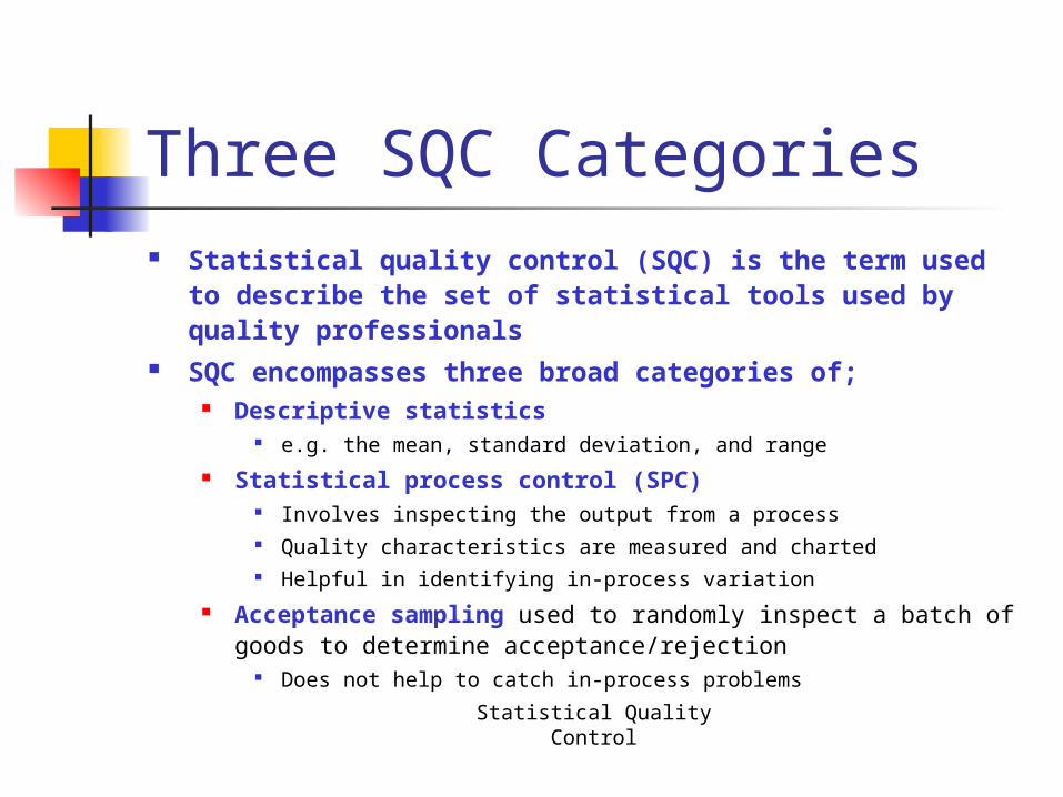
Three SQC Categories Statistical quality control (SQC) is the term used to

describe the set of statistical tools used by quality professionals

SQC encompasses three broad categories of; Descriptive statistics

e.g. the mean, standard deviation, and range Statistical process control (SPC)

Involves inspecting the output from a process Quality characteristics are measured and charted Helpful in identifying in-process variation

Acceptance sampling used to randomly inspect a batch of goods to determine acceptance/rejection

Does not help to catch in-process problems


Sources of Variation Variation exists in all processes. Variation can be categorized as either;

Common or Random causes of variation, or Random causes that we cannot identify Unavoidable e.g. slight differences in process variables like diameter,

weight, service time, temperature

Assignable causes of variation Causes can be identified and eliminated e.g. poor employee training, worn tool, machine needing repair


Traditional Statistical Tools Descriptive Statistics

include The Mean- measure of

central tendency

The Range- difference between largest/smallest observations in a set of data

Standard Deviation measures the amount of data dispersion around mean

Distribution of Data shape Normal or bell shaped or Skewed

n

xx

n

1ii

1n

Xxσ

n

1i

2

i


Distribution of Data Normal

distributions

Skewed distribution

© Wiley 2010

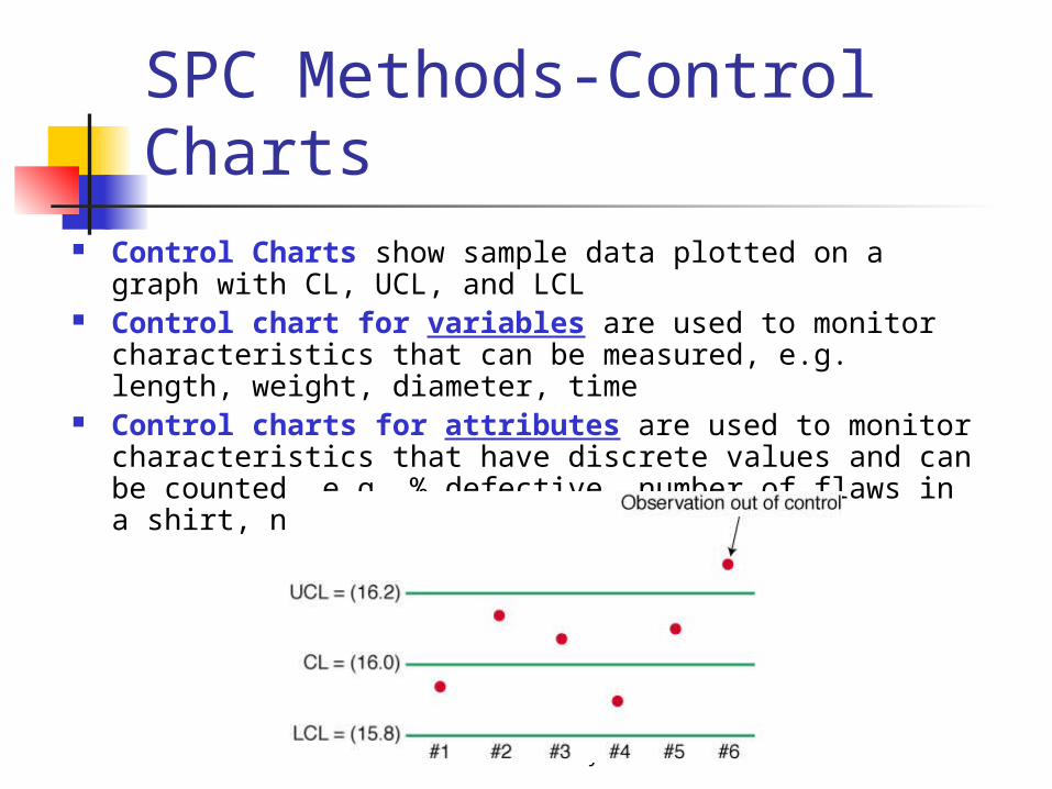
SPC Methods-Control Charts

Control Charts show sample data plotted on a graph with CL, UCL, and LCL

Control chart for variables are used to monitor characteristics that can be measured, e.g. length, weight, diameter, time

Control charts for attributes are used to monitor characteristics that have discrete values and can be counted, e.g. % defective, number of flaws in a shirt, number of broken eggs in a box

Analysis of Patterns on Control Charts

When do you have a problem with your process? One or more points outside of the control limits A run of at least seven points (up, down or above

or below center line) Two or three consecutive points outside the 2-

sigma warning limits, but still inside the control limits

Four or five consecutive points beyond the 1-sigma limits

An unusual or nonrandom pattern in the data

From Douglas C. Montgomery “Introduction to Statistical Quality Control”


Setting Control Limits Percentage of values

under normal curve

Control limits balance

risks like Type I error

Hypothesis Tests Results of hypothesis tests fall into

one of four scenarios:


Type I Error OK

OK Type II Error

Type I and Type II Error ART and BAF

Type I - ART (Alpha, Reject Ho

when true)

Type II - BAF (Beta, Accept Ho

when false)


Jury Trial vs. Hypothesis Test

© Wiley 2007

Defendant isInnocent

Jury Trial Hypothesis Test

Assumption

Standard of Proof

Evidence

Decision

Beyond areasonable doubt

Null hypothesisis true

Facts presentedat trial

Fail to reject assumption (not guilty)

orreject (guilty)

Determined by

Summary statistics

Fail to reject H0

orReject H0 in favor

of Ha

Context? What does it mean to make a type I error

here? Convict an innocent person of a crime.

What does it mean to make a type II error? Fail to convict a guilty person.

What do we usually say about type I and type II error rates in this context?


Control Charts for Variables

Use x-bar and R-bar charts together

Used to monitor different variables

X-bar & R-bar Charts reveal different problems

In statistical control on one chart, out of control on the other chart? OK?


Control Charts for Variables Use x-bar charts to monitor the

changes in the mean of a process (central tendencies)

Use R-bar charts to monitor the dispersion or variability of the process

System can show acceptable central tendencies but unacceptable variability or

System can show acceptable variability but unacceptable central tendencies

Graphical Analysis“A picture is worth a thousand words.”

Graphical analysis is the first step in analyzing your data. Examples: Distribution (histogram, dotplot,

boxplot) Time Series plot for trending I-chart (for Individual data points) Normality Cpk (when applicable) graph

(Minitab)Statistical Quality Control

Dotplot of Tensile Test Data


80757065605550CONTROL

Dotplot of CONTROL

Time Series Plot


70635649423528211471

80

75

70

65

60

55

50

Index

CO

NTR

OL

Time Series Plot of CONTROL

Individuals (I) Chart


71645750433629221581

85

80

75

70

65

60

55

50

Observation

Indiv

idual V

alu

e _X=71.72

UCL=82.74

LCL=60.69

1

1

1

11

1

1

I Chart of CONTROL

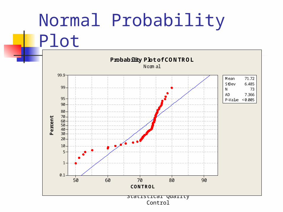
Normal Probability Plot


9080706050

99.9

99

95

90

80706050403020

10

5

1

0.1

CONTROL

Perc

ent

Mean 71.72StDev 6.485N 73AD 7.366P-Value <0.005

Probability Plot of CONTROLNormal

Cpk Graph (Minitab)


847872666054

LSL USL

LSL 65Target *USL 85Sample Mean 71.7151Sample N 73StDev(Within) 3.67538StDev(Overall) 6.4853

Process Data

Cp 0.91CPL 0.61CPU 1.20Cpk 0.61

Pp 0.51PPL 0.35PPU 0.68Ppk 0.35Cpm *

Overall Capability

Potential (Within) Capability

PPM < LSL 123287.67PPM > USL 0.00PPM Total 123287.67

Observed PerformancePPM < LSL 33846.99PPM > USL 150.42PPM Total 33997.41

Exp. Within PerformancePPM < LSL 150234.16PPM > USL 20257.02PPM Total 170491.18

Exp. Overall Performance

WithinOverall

Process Capability of CONTROL

Confidence Statements A confidence statement is used to state the

level of quality of manufactured product. Whether it is dimensional or pass/fail data, confidence statements can help to state the quality level achieved by a process in relation to the specification.

When the true means and standard deviations are not known, estimates of these parameters such as sample standard deviations and sample means are used to make confidence statements based on tolerance limits using either binomial probabilities or k-factors.

There are three types of confidence statements that are primarily used.


Confidence Statements 1. Attribute data confidence statements are used

to state the quality level when data is of a pass/fail type. A binomial probability is used to calculate a 95% confidence statement that at least x% of the population will pass the required specification.

2. Two sided confidence statements are used to describe the quality level of data that has an upper and lower specification limit. The data is assumed to come from a normally distributed population. A two sided tolerance limit table is used for determining probability levels for percent of population. This probability is stated as a 95% confidence that at least x% of the population will be within the specification.


Confidence Statements 3. One sided confidence statements are used to

describe the quality level of data that has either a maximum or minimum specification limit. As with the two sided confidence statement the data is assumed to be from a normally distributed population. A one sided tolerance limit table is used for the probability levels for percent of population in this case. This probability is stated as a 95% confidence that at least x% of the population will be either above the minimum specification or below the maximum specification.


Confidence StatementsFor confidence that data is greater than min specSample mean – K*(sample sd) = min spec

xbar- Ks = min- Ks = min - xbarK = (xbar - min)/s

For confidence that data is less than max specSample mean + K*(sample sd) = max spec

xbar + Ks = maxKs = max - xbar

K = (max - xbar)/s

For two sided tolerance limit both calculations should be made and lowest k-factor compared with table value.


Confidence Statements


Confidence Statements


In the case of attribute data sample size will determine the level that is reached with a confidence statement. The higher the sample size used (with zero or minimal failures), the higher the percent of population is when stating the confidence.

Below is a chart showing how sample sizes can effect the 95% confidence statements:

Percent of Population Defects Sample Size 90 0 30 95 0 60 99 0 300

99.9 0 3,000 99.99 0 30,000

99.999 0 300,000

Sample Size The following simple formula may be used to estimate

sample size (for any distribution) to determine a sample mean, or average, when estimates of the standard deviation are known.


2

22

B

szn

n represents the sample size to be calculated

z represents the table value for the specified confidence desired (i.e., z %)90( = 1.65, z %)95( = 1.96, z %)99( = 2.58)

s represents the estimated standard deviation

B represents the bound of the error of estimation, or ½ of the

desired range of accuracy, e.g., if you desire accuracy of x ± 3 psi, then B = 3 psi.

Sample Size The following simple formula may be used to estimate

sample size to determine a proportion (fraction) defective.

n= p (1-p) (z / B)Where:


n represents the sample size to be calculated.

p represents the estimate of the population fraction defective. If no estimate of p is available, assume worst case of p = 0.5.

z represents the table value for the specified confidence desired (i.e., z %)90( ) = 1.65, z %)95( = 1.96, z %)99( - 2.58).

B represents the bound of the error of estimation, or ½ of the desired range of accuracy, e.g., if you desire accuracy of p ± 0.002.

Sample Size

Example: An engineer wants to estimate a sample size to determine the proportion of unacceptable attributes that may be present in a manufacturing process, e.g., the number of molded components with flash present on the parting line.

If a known history of scrap is already present in a similar product, then that proportion can be used.

If the expected proportion is unknown, then you should use the worst case, or 0.5 as your estimated proportion.

Let’s say the engineer does not know the proportion and uses 0.5 as the estimate.

He/she wants to know at 95% confidence what the sample size should be and is willing to be accurate within ± 0.1.

n = 0.5 (0.5) (1.96/0.1) = 96.04 or rounded up, 97


Process CapabilityProcess Capability Study is an approach to determine the

inherent variability of each process, sub-process, and piece of equipment.

This study provides a method to compare the relationship between the variability of the process and the tolerance range to assure that the process is capable of achieving the tolerance window.

Typically process capability studies occur in five stages; (1) process characterization, (2) metrology characterization, (3) capability determination, (4) optimization or reduction of variability, and (5) preventive control.

The two standard methods for measuring process capability are Cp and CpK.


Process Capability Cp: Process Cp is a numeric index that represents the

inherent capability of a process to meet the requirements of the tolerance range without respect to centeredness. It represents precision, and is calculated as follows:


6

LSLUSLCp

Where:

USL= The Upper Specification Limit

LSL = The Lower Specification Limit

σ = The population standard deviation

Process Capability Cp represents the precision, but not the

accuracy of the process in respect to the tolerance window.


High Accuracy but low precision

High Precision but low Accuracy

Process Capability The 6 is estimated from the process, and

is more accurate as the sample size gets larger.

Decisions about process capability may not be valid with data from a single run, and when possible, should be based on data from 2 or more runs.

Cp is only valid when the distribution of the data is statistically normal.

Outliers, bimodal tendencies and skewness may lower the Cp value.


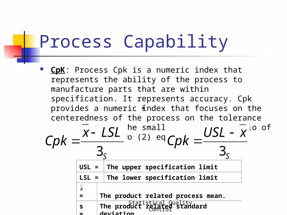
Process Capability CpK: Process Cpk is a numeric index that represents

the ability of the process to manufacture parts that are within specification. It represents accuracy. Cpk provides a numeric index that focuses on the centeredness of the process on the tolerance window. Cpk is the smallest resulting ratio of the following two (2) equations:


S

LSLxCpk

3

S

xUSLCpk

3

USL = The upper specification limit

LSL = The lower specification limit

= The product related process mean.

s = The product related standard deviation

xxx

x

Process Capability A machine or process is sometimes referred to as

being capable when its Cpk has a minimum value of one (1.00) and when process stability has been proven.

A Cpk equal to one (1.00) implies that 99.73% of the product is within specification limits, provided that the process is stable. However, it should be noted that if the machine capability is only 1.0, it will be impossible to maintain a Cpk of 1.0 or higher.

The goal should be a Cp as high as possible. It is possible for a process to have a high Cp, but a low

Cpk, if the process is not centered in the tolerance window. A Cpk of 1.33 or higher should be targeted.


CpK A CpK of 1.33 means that the difference

between the mean and specification limit is 4σ (since 1.33 is 4/3).

With a CpK of 1.33, 99.994% of the product is within the within specification.

Similarly a CpK of 2.0 is 6σ between the mean and specification limit (since 2.0 is 6/3).

With a CpK of 2.0 99.9999998% of the product is within specification.



Acceptance Sampling Definition: the third branch of SQC refers to the

process of randomly inspecting a certain number of items from a lot or batch in order to decide whether to accept or reject the entire batch

Different from SPC because acceptance sampling is performed either before or after the process rather than during

Sampling before typically is done to supplier material Sampling after involves sampling finished items before

shipment or finished components prior to assembly Used where inspection is expensive, volume is

high, or inspection is destructive


Acceptance Sampling Plans Goal of Acceptance Sampling plans is to determine the

criteria for acceptance or rejection based on: Size of the lot (N)

Size of the sample (n)

Number of defects above which a lot will be rejected (c)

Level of confidence we wish to attain

There are single, double, and multiple sampling plans Which one to use is based on cost involved, time consumed, and

cost of passing on a defective item

Can be used on either variable or attribute measures,

but more commonly used for attributes

Acceptance Sampling Plans

ANSI/ASQC Z1.4 (Attribute or P/F Data)

ANSI/ASQC Z1.9 (Variable Data) C=0 (Attribute, reject on 1) MIL STD 1235C (Continuous

Production)


Sample Size Calculation –Z 1.4

© Wiley 2007

Sampling Plan for Normal Inspection

© Wiley 2007

AQL Inspector’s Rule

© Wiley 2007

AQL Inspector’s Rule

© Wiley 2007

Accept/Reject

Sample Size


Acceptance Sampling Plans

• As mentioned acceptance sampling can reject “good” lots and accept “bad” lots. More formally:

Producers risk refers to the probability of rejecting a good lot. In order to calculate this probability there must be a numerical definition as to what constitutes “good”

– AQL (Acceptable Quality Limit) - the numerical definition of a good lot. The ANSI/ASQC standard describes AQL as “the maximum percentage or proportion of nonconforming items or number of nonconformities in a batch that can be considered satisfactory as a process average”

• Consumers Risk refers to the probability of accepting a bad lot where:– LTPD (Lot Tolerance Percent Defective) - the numerical definition of a bad lot

described by the ANSI/ASQC standard as “the percentage or proportion of nonconforming items or noncomformities in a batch for which the customer wishes the probability of acceptance to be a specified low value.

Acceptance Sampling

© Wiley 2007

0

0.2

0.4

0.6

0.8

1

1.2

Prob

abili

ty o

f Acc

epta

nce

Percent Defective

OC Curve

LTPDAQL

Producers Risk

Consumers Risk


Implications for Managers How much and how often to inspect?

Consider product cost and product volume Consider process stability Consider lot size

Where to inspect? Inbound materials Finished products Prior to costly processing

Which tools to use? Control charts are best used for in-process production Acceptance sampling is best used for

inbound/outbound


SQC Across the Organization SQC requires input from other organizational

functions, influences their success, and are actually used in designing and evaluating their tasks

Marketing – provides information on current and future quality standards

Finance – responsible for placing financial values on SQC efforts

Human resources – the role of workers change with SQC implementation. Requires workers with right skills

Information systems – makes SQC information accessible for all.

Quality Control

© Wiley 2007

Documents

Statistical Quality Control by R.B. Clough – UNH M. E. Henrie - UAA