Statistical properties of aftershock rate decay: Implications for the assessment of continuing activity

Acta Geophysica vol. 59, no. 4, Aug. 2011, pp. 748-769

DOI: 10.2478/s11600-011-0016-2

________________________________________________ © 2011 Institute of Geophysics, Polish Academy of Sciences

Statistical Properties of Aftershock Rate Decay: Implications for the Assessment

of Continuing Activity

Aggeliki ADAMAKI1, Eleftheria E. PAPADIMITRIOU1, George M. TSAKLIDIS2, and Vassilios KARAKOSTAS1

1Geophysics Department, Aristotle University of Thessaloniki, Thessaloniki, Greece e-mails: [email protected], [email protected], [email protected]

2Department of Statistics and Operational Research, Aristotle University of Thessaloniki, Thessaloniki, Greece

e-mail: [email protected]

A b s t r a c t

Aftershock rates seem to follow a power law decay, but the assess-ment of the aftershock frequency immediately after an earthquake, as well as during the evolution of a seismic excitation remains a demand for the imminent seismic hazard. The purpose of this work is to study the temporal distribution of triggered earthquakes in short time scales fol-lowing a strong event, and thus a multiple seismic sequence was chosen for this purpose. Statistical models are applied to the 1981 Corinth Gulf sequence, comprising three strong (M = 6.7, M = 6.5, and M = 6.3) events between 24 February and 4 March. The non-homogeneous Pois-son process outperforms the simple Poisson process in order to model the aftershock sequence, whereas the Weibull process is more appropriate to capture the features of the short-term behavior, but not the most proper for describing the seismicity in long term. The aftershock data defines a smooth curve of the declining rate and a long-tail theoretical model is more appropriate to fit the data than a rapidly declining exponential func-tion, as supported by the quantitative results derived from the survival function. An autoregressive model is also applied to the seismic se-quence, shedding more light on the stationarity of the time series.

Key words: aftershock rate changes, decay forecasting, Greece.

STATISTICAL PROPERTIES OF AFTERSHOCK RATE DECAY

749

1. INTRODUCTION Given the threat posed by aftershocks in an area already hit by a strong main shock, it is of paramount importance for seismic hazard assessment purposes to model the expected occurrence rate of the aftershock sequences. The strongest aftershocks oftentimes occur late after the main event, and for this reason the time window selected for this purpose in the current paper is long enough compared with what is usually defined as aftershock period, that is, a period of several weeks or months. It is commonly accepted that aftershock activity, meaning activity significantly higher than before the main shock occurrence, lasts for years and even decades, and that an aftershock produced at any time may be large (Lomnitz 1966).

Several researchers focus on the application of the probability theory in seismic sequences in order to study the temporal and spatial distribution of induced seismicity that follows a strong earthquake, starting from the well- known Omori law for aftershocks describing the power law decay of seis-micity after an earthquake. A useful tool for the statistical analysis of this kind of data is a point process which can be used to model random events in time. Several point-process models have been proposed (Vere-Jones 1992, Ogata 1999, among others) in which each point represents the time and place of an event and several attempts have been made to assess the seismicity rate changes caused by a strong event. A simple approach to the phenomenon is to consider a homogeneous process, taking into account the previous seis-micity (Toda et al. 1998, 2002), which underestimates the rate changes (Marsan 2003, Felzer et al. 2003). In these cases, the homogeneous process is not directly applicable and data heterogeneity is removed using decluster-ing techniques (Matthews and Reasenberg 1988, Kilb et al. 2000, Gomberg et al. 2001, Wyss and Wiemer 2000). On the other hand, the aftershocks are a considerable part of a seismic sequence, including important information about changes in the seismicity rate and for this reason significant research devoted to the modeling of aftershock occurrence and its impact to the re-gional seismicity has been done.

A homogeneous Poisson process was tested by Wyss and Toya (2000) as the point process that can describe the earthquake occurrence characterized by a constant rate in time scale of decades. The authors did not use any dec-lustering techniques, although some of these methods yield to a homogene-ous Poisson process (Gardner and Knopoff 1974, Reasenberg 1985). They also used the chi-square test, splitting the data into groups of a fixed number of events. The result was to reject the null hypothesis for the homogeneous Poisson process only in a small percentage of the cases.

Marsan (2003) tested three seismic sequences to assess rate changes caused by a strong earthquake. He observed that over a period of 100 days

A. ADAMAKI et al.

750

after the main shock it was not easy to observe the phenomenon of seismic quiescence. Of course, in long-time scales it is even more difficult to proper-ly assess whether the rate changes are due to a previous strong event or not. Firstly, a Poisson process with rate λ(t) is introduced, which can be either constant (homogeneous Poisson process) or given as a function of time, whereas the second case is a non-homogeneous Poisson process. In this work a power law model (Utsu 1970) was also tested, which is a generaliza-tion of the model of Ogata and Shimazaki (1984) and Woessner et al. (2004). Finally, an autoregressive model was applied, which led to a syste-matic overestimation of future values of the seismicity rate during the after-shock sequences. Marsan and Nalbant (2005) analyzed the steps of the method that has to be followed in order to estimate the parameters of several models and then correlated the results with the observed changes in Coulomb stress.

Ogata (2005a, b) also investigated a point process model (Daley and Vere-Jones 2003) which introduces the seismicity rate as a function of the form λθ(t) (where θ stands for the characterizing parameters of the rate),

Fig. 1. Main seismotectonic properties of the Aegean and the surrounding area: NAF – North Anatolian Fault, NAT – North Aegean Trough, CTF – Cephalonia Transform Fault, and RTF – Rhodes Transform Fault. Rectangle indicates the study area. Colour version of this figure is available in electronic edition only.


751

depending on time, t. The rate λθ(t) depends not only on the elapsed time (as for example, the modified Omori law) but also on the occurrence times and the size of previous events. In order to test the fitting quality of the model in each seismic sequence, the cumulative number of earthquakes is compared to the theoretical values estimated from the models.

The purpose of this article is to use earthquake statistics to investigate whether we may use part of the data comprising a seismic sequence, in order to evaluate the temporal evolution of the imminent seismic activity. In order to perform this investigation, it is necessary to seek for the appropriate statis-tical tools. Our objective is to capture the main features of an aftershock se-quence through a number of appropriate approaches.

Considering the seismic sequences as stochastic point processes, three statistical models were chosen to apply to a multiplet that occurred in 1981 in the Corinth Gulf (shown by a rectangle in Fig. 1), a rapidly extended half graben which has experienced several destructive earthquakes both in histor-ical times and the recent decades. As in most relevant investigations, the spa-tial distribution of aftershocks was considered stationary in time, and changes in the rate at which events occur is explored, not where they occur. After defining the model parameters, tests were performed in order to show whether they are supported by the data.

2. METHODOLOGY Estimation of the seismicity rate changes caused by a strong earthquake is based upon the assumption that the earthquake occurrence can be described by stochastic processes, e.g., a Poisson point process. A Poisson distribution is a discrete probability distribution expressing the probability for the occurrence of a certain number of events occurring during a specific time interval, when the average occurrence rate is known and these events are independent of the time of the last event. Knowing that the expected number of occurrences within the specific time interval is equal to λ, the probability of having exactly k-occurrences is given by

( ) ,!

k ef kk

λλλ−

= (1)

where k ∈ N, giving the number of occurrences, λ ≥ 0, and λ ∈ R represent-ing the expected number of observations within the given time period. Equa-tion (1) represents the probability mass function of a Poisson distribution. The cumulative density function is given by

0

( ) .!

ik

i

F k ei

λ λλ −

=

= ∑ (2)

A. ADAMAKI et al.

752

A Poisson distribution is used to describe a phenomenon that can be as-sumed as a Poisson process. A discrete process, {Ν(t), t ≥ 0}, where N(t) ∈ N is called a Poisson process with rate λ, λ > 0, if

it is Ν(0) = 0, when t = 0, the number of occurrences within each time interval Δt is indepen-

dent of the number of occurrences within any other irrelevant time interval, the number of events occurring within any time interval of length t

can be approached by the Poisson distribution with mean value λ × t. Assuming times, s and s + t , we get

{ } ( )( ) ( ) , 0 .!

nt tP N t s N s n e n

nλ λ−+ − = = ≥ (3)

If the rate parameter is time-dependent, λ(t), then the expected number of events of the Poisson process in the time interval [t, t + δ] is given by

[ , ] ( )d .t

t

t t s sδ

λ δ λ+

+ = ∫ (4)

The Poisson process can be defined by the seismicity rate λ(t) coming up from the time period [0, Τ] under study and the observed earthquake times, ti , i.e., the realizations of this Poisson process.

It is known that the waiting times (inter-arrival times) of a Poisson process are exponentially distributed. The probability density function of the exponential distribution is given by

11 for 0( )

0 for 0

xe x

f xx

μ

μ μ

−⎧≥⎪= ⎨

⎪ <⎩

(5)

where μ is the scale parameter of the distribution and is the reciprocal of the Poisson parameter, λ. The expected survival duration of the system, i.e., the mean inter-arrival time of subsequent events, is equal to μ.

A Poisson process with constant rate λ, i.e., a time-independent rate, is known as a homogeneous Poisson process. In this case, the waiting times of the point process are exponentially distributed with a mean μ = 1/λ. The ex-pected number of earthquakes in any interval of length t equals λ × t, and the probability that there are exactly n-occurrences in this interval is given by

( )( ) , 0, 1, 2,... .!

nt tP n t e n

nλ λλ −= = (6)

By replacing the constant λ with a function λ(t), which gives the rate of earthquakes at time, t, the process becomes a non-homogeneous Poisson


753

process. In this case, the number of earthquakes in any interval is time de-pendent, and the mean rate in an interval [t, t + Δt] is given by eq. (4). The probability that there are exactly n-occurrences within the specific interval is then given by

( , )[ , ]

[ , ]( ) , 0, 1, 2,... .!

nt t t

t t tt t tP n n e n

nλ λ− +Δ

+Δ

+ Δ= = = (7)

Two functions expressing the rate λ(t) are tested in the present study, namely

( ) a btt eλ += (8) and 1( ) b bt a btλ − −= , (9)

both selected because they allow the rate decaying as time passes. More spe-cifically, the rate function λ(t) given by eq. (8) decays rapidly to zero while λ(t) given by eq. (9) may decay smoothly to 0 (by a suitable choice of the parameters).

In order to apply those models to the data of a seismic sequence, a spe-cific region must be selected, with dimensions a few times larger than the main rupture length. Determining the study area, the threshold magnitude must be defined to ensure the completeness of the data set. The next step is to define the duration of the earthquake catalog, which depends on the pur-pose of the specific study. Naming T0 the time of the main shock occurrence, the catalog expands within the intervals [0, T0] and [T0, T], where T is lo-cated several days after T0. The lengths of the time intervals between con-secutive events occurring at times ti (t0 = T0) are computed and their distribution is tested using the chi-square test; in our case the null hypothesis is that the inter-arrival times are exponentially distributed. This fact is tested separately for consecutive sub-intervals of the data set periods [0, T0] and [T0, T]. If the null hypothesis is accepted for a tested sub-interval, then the number of occurrences in this sub-interval follows a Poisson distribution with a specific constant rate parameter (homogeneous Poisson process). The data in each sub-interval are divided into groups (cells) based on the lengths of the inter-arrival times and the expected frequencies are estimated for each group of inter-arrival times. In order to apply the chi-square test, attention is paid in defining the groups such that the expected frequency in each group is greater than 5.

Especially for the period [T0, T], since the aftershock rate over the first few days after the main shock (which is very high compared with the rate in the previous time interval [0, T0]) is characterized by strong changes, (differ-ent) constant rates are assumed over short sub-intervals of [T0, T]. Thus, the

A. ADAMAKI et al.

754

interval [T0, T] is divided into short intervals [Ti-1, Ti], i ∈ N+, each one tested for its homogeneity as a Poisson process with a rate parameter, λi (using the chi-square test). Note that each λi is computed taking into consideration the number of events in the respective sub-interval [Ti-1, Ti], which is not neces-sarily equal for all sub-intervals. The set {λi , [(Ti-1 + Ti)/2]}, i ∈ N+, is then used as the input data set to fit a selected curve λ(t) that best describes the evolution of the seismicity rate within the entire period [T0, T]. In the present study a rate function of the form λ(t) = ea + bt is fitted to the data set {λi , [(Ti-1 + Ti)/2]}, i ∈ N+, where the parameters a and b are estimated by the least squares’ method.

Finally, the non-homogeneous Poisson process is assumed to have a rate function of the form λ(t) = a–b btb–1; the parameters a and b are estimated by the maximum likelihood method using the time of occurrence, ti , of each earthquake. This rate function can be an increasing or decreasing function, according to whether b > 1 or b < 1, respectively. Based on the form of λ(t), the aforementioned process is named a process with a Weibull hazard rate or simply a Weibull process. The special case of b = 1 leads to a constant ha-zard rate, which corresponds to the exponential case characterized by the memoryless property. The maximum likelihood estimators for a and b are given by

1/ 1

1

, ,ln( / )

nb n

n ii

t na bn t t

−

=

= =

∑ (10)

where n stands for the number of data and ti denotes the time of occurrence of the i-th earthquake, i = 1, 2, …, n.

One more way to model the sequence of earthquakes is to consider a random variable Z(t), representing the number of earthquake occurrences at any time, t. The set {Z(t)} constitutes a time series, i.e., a family of stochastic processes. The model which is fitted to the data is the autoregressive model of order p, p ∈ N+, abbreviated as AR(p). The AR(p) model assumes that

1

,P

t i t i ti

Z Z aφ −=

= +∑ (11)

where φi are the unknown parameters and at is a white noise function with a zero mean and variance σ2. The time series is considered to be stationary. Then the parameters φi can be estimated using several methods, e.g., the Yule–Walker equations, which constitute a set of linear equations relating the un-known parameters with the autocorrelations. Then

1 1 2 2 ... ,p p p pρ φ ρ φ ρ φ− −= + + + (12)


755

where the coefficients ρi , i = 1, 2, …, p – 1, stand for the autocorrelations which describe the correlations of the values of the process against a time-shifted version of themselves.

The aforementioned methodologies concerning the Poisson processes and the AR(p) model are explained in detail in Section 4.

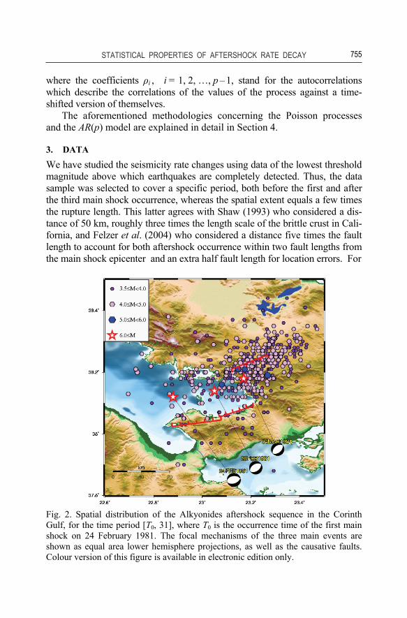
3. DATA We have studied the seismicity rate changes using data of the lowest threshold magnitude above which earthquakes are completely detected. Thus, the data sample was selected to cover a specific period, both before the first and after the third main shock occurrence, whereas the spatial extent equals a few times the rupture length. This latter agrees with Shaw (1993) who considered a dis-tance of 50 km, roughly three times the length scale of the brittle crust in Cali-fornia, and Felzer et al. (2004) who considered a distance five times the fault length to account for both aftershock occurrence within two fault lengths from the main shock epicenter and an extra half fault length for location errors. For

Fig. 2. Spatial distribution of the Alkyonides aftershock sequence in the Corinth Gulf, for the time period [T0, 31], where T0 is the occurrence time of the first main shock on 24 February 1981. The focal mechanisms of the three main events are shown as equal area lower hemisphere projections, as well as the causative faults. Colour version of this figure is available in electronic edition only.

A. ADAMAKI et al.

756

the area of Greece, Karakostas (2009) has found that the pre-stress area, namely the preparation area of an incoming strong event, is rather equal to three times the fault length.

It is now widely accepted that many earthquakes are triggered by their preceding counterparts: not only aftershocks by the main shocks of the se-quence they belong, but also stronger events by smaller ones. In this respect, we decided to go back in time and investigate any possible indication for the first main shock occurrence, from the behavior of small magnitude seismici-ty. The data were taken from the Greek National Seismological Network and were compiled from the bulletins of the Central Seismological Station of Geophysics Department of the Aristotle University of Thessaloniki (http://geophysics.geo.auth.gr/ss/). The completeness of the data set was checked using the Gutenberg–Richter relation and the minimum magnitude above which the sample is complete was found equal to 3.5. The catalog is separated into two parts, with the first period covering the interval from 1979 up to the occurrence time of the first main shock (set as T0). This was chosen long enough to give an adequate data set (116 events) so that the simplest time-invariant model could be applied on these data. The second period lasts for 1040 days since T0 (784 earthquakes with M ≥ 3.5) and was used for the application of the time-dependent models. Both periods concern the area of the Corinth Gulf, shown in Fig. 2.

4. RESULTS The application of the methodology presented in the previous section to the aforementioned seismic sequence and the corresponding data set is analyzed, starting with the assumption that the earthquake number within a given time interval can be modeled as a Poisson random variable of mean rate, λ. The simplest approach, namely the homogeneous Poisson model, which assumes constant rate, λ, is first applied. Plotting the cumulative number of earthquakes against time, reveals that the activity before the first main shock can be mod-eled as a homogeneous Poisson process (Fig. 3), since the slope of the curve representing the cumulative number of earthquakes is relatively constant. The goodness of fit of the homogeneous Poisson model to the data is tested by means of the chi-square test, in order to find out whether it is reasonable or not to assume that this part of the sequence can be modeled as a homogeneous process. The null hypothesis, H0, is that the inter-arrival times are exponen-tially distributed and therefore the point process is a homogeneous Poisson process. Several subsequent periods were tested, always being long enough in order to have the appropriate number of data for using the chi-square test.

For each case the value of the parameter μ of the exponential distribution was firstly estimated, using the inter-arrival times of the earthquakes and the


757

Fig. 3. Cumulative number of earthquakes against time in the area of the Corinth Gulf, for the time interval from 1 January 1979 to 31 December 1983. Colour ver-sion of this figure is available in electronic edition only.

maximum likelihood method. The data set was divided into 3 cells (i.e., 1 degree of freedom) and the expected frequencies were found; then they were used to get the chi-square statistic, χ2. The critical value, x2

, for our case (1 de-gree of freedom and the significance level equal to 0.025) is equal to 5.02 and thus H0 is accepted when χ2 is lower than this value. Finally, in each of the subsequent periods the seismicity rate, λ, was estimated using the maximum likelihood method, leading to values with no significant numerical deviations.

For example, for the two time intervals with (common) right endpoint T0 and lengths equal to 251 and 391 days, the values of the seismicity rates are found to be λ1 = 0.1434 and λ2 = 0.1458, respectively, which are very close to each other as well as to the slope of the curve representing the cumulative number of earthquakes for the period [0, T0], see Fig. 3. Table 1 summarizes the results of the chi-square test for the two periods tested here. A simple

Table 1 The results of chi-square test applied to the data

preceding the first strong event of the earthquake sequence

Time interval Observations Statistical χ2 μ λ

[–251, Τ0] 36 1.4968 6.9570 0.1434 [–391, Τ0] 57 3.9310 6.8542 0.1458

Explanations: μ – value of the exponential distributions of the inter-arrival times, λ – seismicity rate of the respective Poisson distributions. Critical value x2 = 5.02, d.f. = 1, a = 0.025.

A. ADAMAKI et al.

758

Fig. 4. Simulation of the homogeneous poisson process (light dashed line) with rate: (a) λ1 = 0.1434 estimated from the data of the interval of 251 days before the first strong earthquake, and (b) λ2 = 0.1458 estimated from the data of the last 391 days before T0. The real data curve is shown with a thick solid line. Colour version of this figure is available in electronic edition only.

algorithm, which uses a random number generator of the exponential distribu-tion for the theoretical inter-arrival times, is then used in order to model the above two homogeneous parts using the previous values of the seismicity rate. This simulation is presented in Fig. 4, where the real data curve is very close to the theoretical one, pointing to an adequate fitting of the model as the seis-micity rate in this part is characterized by linearity.

As it is shown in Fig. 3, the seismicity rate changes cannot be assumed to be constant for the period following T0, i.e., the occurrence time of the first main shock. In order to model the events of this time interval, it is necessary to introduce a non-homogeneous Poisson process, where the rate λ is no longer constant in time and constitutes a function of time, λ(t). A non-homogeneous Poisson process can be divided in subsequent homogeneous processes of short length, each one characterized by a specific rate, λi. The time interval of the aftershock sequence then splits into subsequent shorter time intervals that are tested for their homogeneity using the chi-square test and the rates λi are estimated using the events of each interval. Based on this method, the data of the first month of the aftershock sequence are divided into 16 intervals with rates λi in order to have the appropriate number of data in each interval to test the null hypothesis. Table 2 summarizes the results of the test for the 16 subsequent time periods. The seismicity rates are plotted against time in Fig. 5. Generally, it is observed that the values of λi decrease as time passes for both periods that follow the strong earthquakes of the se-quence. It is remarkable in this part that the rate λ increases just before the occurrence time of the third strong event. This is shown in the marked area


759

Table 2 The results of chi-square test applied to the data

preceding the first strong event of the earthquake sequence

Time interval Observations Statistical χ2 μ λ

(0, 0.15] 31 0.7542 0.0046 206.6667 (0.15, 0.3] 29 1.4461 0.0053 193.3333 (0.3, 0.6] 35 1.2113 0.0113 116.6667 (0.6, 1] 31 0.7029 0.0094 77.5000 (1, 2] 33 0.5434 0.0308 33.0000 (2, 3] 20 2.8833 0.0450 20.0000 (3, 6] 28 4.8783 0.1086 9.3333 (6, 8.045] 25 0.2228 0.0842 12.5000 (8.045, 8.15] 36 0.2572 0.0026 234.3750 (8.15, 8.5] 40 0.2363 0.0087 114.2857 (8.5, 9] 21 1.1854 0.0222 42.0000 (9, 11] 34 1.6289 0.0591 17.0000 (11, 14] 31 2.8419 0.0976 10.3333 (14, 17] 25 0.2782 0.1078 8.3333 (17, 22] 32 1.1051 0.1607 6.4000 (22, 31] 30 0.8960 0.2945 3.3333

Explanations: μ – value of the exponential distributions of the inter-arrival times, λ – seismicity rate of the respective Poisson distributions. Critical value x2 = 5.02, d.f. = 1, a = 0.025.

of the plot in Fig. 5 and constitutes a first indication of foreshock activity increase before the third main event.

Because of the fact that the characteristic rate decrease is interrupted by the occurrence of a strong earthquake almost eight days after the first one, the statistical models are applied to two different periods, the one that fol-lows time T0 (time where the first two strong events occurred) and the second one following the third strong earthquake of the sequence. For each short time interval, the Poisson rate parameter corresponds to the center of the interval (as shown in Fig. 6).

Figure 6 gives evidence to assume that the declining seismicity rate tends to an exponential decaying mode. In order to model the time dependence of the seismicity rate, the form given by eq. (8) is first tested. In this case, the least-squares method is used to estimate the values of the parameters a and b

A. ADAMAKI et al.

760

Fig. 5. Occurrence rates, λi, plotted versus time for the time period [T0, 31], which continuously decay up to the 6th day. The area marked with rectangle shows the in-creasing rate λ8 of the last homogeneous Poisson process just before the occurrence time of the third strong event of the sequence. After that, the rate abruptly increases, incorporating the first day aftershocks, and then again decreases towards the values observed before T0. Colour version of this figure is available in electronic edition only.

Fig. 6. The polygonal chain (dashed line) connects the values of the Poisson rate pa-rameter corresponding to the center of its interval: (a) during the time period [T0, 8], and (b) for 23 days after the occurrence of the third strong event of the sequence. Colour version of this figure is available in electronic edition only.

of the theoretical exponential curve expressed by ea + bt. Using the initial seven values of the Poisson rate parameters, the theoretical curve is obtained as shown in Fig. 7a, giving the visual results of the model. Besides this qual-


761

Fig. 7. Time series of the sequence (thick line) and simulation curve (thin line). Aftershock rate is given as estimated in Fig. 5. The theoretical curve ea + bt is fitted on the polygonal chains of Fig. 6, using the least-squares method: (a) during the time period [T0, 8], and (b) for 17 days after the occurrence of the third strong event of the sequence. Colour version of this figure is available in electronic edition only.

itative analysis, we also need quantitative results in order to test the goodness of fit. The survival function is then used to estimate the probability of having more than 125 events during the first day of the aftershock sequence and comes up equal to 0.63, whereas the observed number of data is equal to 126. There are 33 events during the second day, and according to the model the probability of having more than 30 events is equal to 0.64. During the third day, however, 20 events occurred, while the model yields the probability of having more than 15 events approximately equal to zero. Thus the model un-derestimates the number of events during the third day, and this can be verified to hold also for the days that follow.

Using the data of the second part of the aftershock sequence (Figs. 6b and 7b) the results are similar to the previous ones of the first part of the se-quence. It is inappropriate then to use the specific exponential form of the Poisson rate λ in order to model the process for longer periods than those of the first few days. For example, using the a and b values as estimated from the six values of the rate parameter shown in Fig. 7b, the survival function is estimated for several time intervals. During the ninth day of the sequence, the probability of having more than 95 earthquakes is found to be equal to 0.66 and the events were 97. During the day that follows, the probability of having more than 5 events is equal to 0.68 but the observed number of earth-quakes is larger (i.e., 16) showing that the model underestimates the real process with a faster onset of the power law decay.

The exponential form cannot be used for longer periods. Thus we next adopt a Weibull form to express the rate function. Integration of λ(t) within

A. ADAMAKI et al.

762

specific time intervals yields the estimated earthquake number which can be then compared to the observed number of the data. Furthermore, the estima-tion of the survival function for each interval can give the probability of hav-ing more than a specific number of events, which can be useful while trying to forecast the evolution of the earthquake generation. As it is shown in the previous section, the parameters a and b are calculated using the maximum likelihood method for various data sets. Figure 8 shows the theoretical and the observed cumulative number of earthquakes during the periods that fol-low the first and the last strong event of the sequence. Taking more data into account, the theoretical curve resulting from the Weibull process approaches the observed data curve providing a better approximation to the real process. In the two marked areas shown in Fig. 8, the best fit of the modeled to the observed curve is shown. By estimating the parameters from the data of the first six days that follow the first strong event, the probability of having more than 205 events within this time interval is found to be 0.69 and the real data are equal to 207. The model provides a good approach, so the next step is to estimate the process during the days that follow. For the eighth day of the sequence the probability of expecting more than 12 earthquakes is equal to 0.58, while the real number is 12. As time passes the model turns out to overestimate the expected number of earthquakes.

Fig. 8. Cumulative number of earthquakes for the Weibull-rates case for different datasets concerning the time periods [T0, 1], [T0, 2], [T0, 3], [T0, 6], and [T0, 8] for the curves named as Fit1, Fit2, Fit3, Fit4, and Fit5, respectively. The thick solid line represents the observed cumulative number of events. Colour version of this figure is available in electronic edition only.


763

Fig. 9. Cumulative number of earthquakes for the Weibull-rates case for different datasets concerning the time periods with lengths equal to 1, 2, 3, 4, 5, and 23 days after the occurrence of the third strong earthquake of the sequence, for the curves named as Fit1, Fit2, Fit3, Fit4, Fit5, and Fit6, respectively. The thick solid line represents the observed cumulative number of events. Colour version of this figure is available in electronic edition only.

The same procedure is presented for the data of the time period that fol-lows the third strong event almost eight days after the first one. In Figure 9 it is obvious that the theoretical curve coming up from the data of the first 5 days fits well the data for a long period. Using the survival function, the probability of having more than 145 earthquakes during this interval is esti-mated to be equal to 0.66 and the observed number of data is equal to 150. By extrapolating the rate λ(t) during the day that follows, the estimated num-ber of events comes close to the observed (which is equal to 12) and the probability of having more than 10 earthquakes comes up equal to 0.57. It is then safe to assume that this model provides a better approximation to the real process than the model with intensity rate λ(t) = ea + bt, and can be used for assessing the continuing seismic activity.

The models applied so far, besides giving additional information about the seismic sequence and its temporal evolution, cannot always yield to the efficient simulation of the seismic behavior. Therefore, the autoregressive model, AR(p), was chosen as a typical statistical tool to analyze the data of the time series of the seismic sequence in order to achieve prediction of its future values. For the application it is necessary to use part of the data to cal-culate the model parameters, and then using these parameters to proceed to the

A. ADAMAKI et al.

764

Fig. 10: (a) Sample autocorrelation function (ACF), and (b) sample partial autocor-relation function (PACF) for the time period [T0, 5.5]. Lags correspond to the num-ber of the elements of the ACF and PACF that are estimated, and horizontal lines show the bounds of the appropriate values. Colour version of this figure is available in electronic edition only.

Fig. 11. Simulation of the autoregressive model (solid line) compared to the real time series (line with crosses) for the time period [T0, 9]. Colour version of this fig-ure is available in electronic edition only.

estimations for the evolving process. In Figure 10 the correlograms show the partial autocorrelation coefficients as well as the autocorrelation function, estimated using the data of the first 5.5 days following T0. The form of the autocorrelation function in this figure testifies the stationarity of the time se-ries, which is a precondition for the application of the autoregressive


765

model. Next, by taking the partial autocorrelation coefficients into account, we conclude that the order p of the model is equal to 2. The next step is to use the Yule–Walker equations to estimate the parameters φi of the model. According to this, the model equation becomes zt = 0.6187 × zt–1 + 0.2063 × zt–2 and Fig. 11 presents a simulation of the AR(2) model. Com-parison of the resulted pattern to the observed time series demonstrates that the model leads to a systematic overestimation of the aftershock sequence.

Fig. 12: (a) Sample autocorrelation function (ACF), and (b) sample partial autocor-relation function (PACF) for the five days interval just after the occurrence of the third strong earthquake. Lags correspond to the number of the elements of the ACF and PACF that are estimated, and the horizontal lines show the bounds of the appro-priate values. Colour version of this figure is available in electronic edition only.

Fig. 13. Simulation of the autoregressive model (solid line) compared to the real time series (line with crosses) for 23 days after the occurrence of the third strong earthquake. Colour version of this figure is available in electronic edition only.

A. ADAMAKI et al.

766

The autoregressive model is then applied to the data of the sequence that follows the third strong earthquake. The results are similar to the previous ones. The estimation of the autocorrelation function gives evidence for the stationarity of the time series while the partial autocorrelation coefficients indicate that the model is of order 2 (Fig. 12). Using the data of the first five days, the Yule–Walker equations lead to zt = 0.6692 × zt–1 + 0.0343 × zt–2 (Fig. 13). The model does not fit well the data because the main part of the estimated curve lies above the respective curve of the observed values. 5. DISCUSSION AND CONCLUSIONS Aftershock activity constitutes one of the largest risks in the aftermath of an earthquake. Aftershocks shake already weakened structures, and if an after-shock is closer to a population center than the original rupture it may cause even more severe local shaking. In our case the second main shock occurred a few hours after and closer to populated areas than the first one, and thus con-tributed mostly to the calamities caused during the first hours of the seismic excitation, whereas the third main shock that occurred on 4 March (M = 6.3) caused substantially more damage in an area intact from the first two main shocks, which are associated with the north-dipping faults located along the southern coastline. For this third main event our analysis revealed a short-term relative quiescence, which is occasionally observed before a large aftershock the rupture of which extends beyond the source of the main event (Matsu’ura 1986, Ogata 2001). This is the case of our studied sequence, concerning in particular the third main shock occurrence.

Our aim was to apply models that would enable us to assimilate the actual seismicity rate, whereas on the other hand to detect anomalous tem-poral deviation of the modeled occurrence rate from the actual one. The models we applied ignored the spatial factor, which could be taken into ac-count with a parallel approximation. In our approach it is assumed that the values of the parameters do not change spatially, even though it is not effi-cient to demonstrate that the differences resulted with changing the study area or magnitude threshold, will not be significant. It is documented that the spatial and temporal distribution of aftershocks is separable into a depen-dence on space and a dependence on time (Shaw 1993).

In order to study the short-term triggered seismicity, three statistical models were applied to the data. We have started with a Poisson process in an attempt to simulate seismicity behavior both before the first main shock and after the third main shock occurrence. The earthquake sequence was initially divided into two parts, one before the first strong event, T0, and the other one after T0. In order to apply the homogeneous Poisson model to the first part, the chi-square test was used for several periods. The values of the seismicity rate, λ, calculated from the data of each of these sub-intervals did


767

not differ significantly and the whole preceding time period could be considered as a homogeneous Poisson process of constant seismicity rate. The second part of the sequence was also divided in subsequent sub-intervals with different seismicity rates. The null hypothesis of the exponential distribution of time intervals was verified for all the cases and it was observed that the value of λ8 corresponding to the eighth sub-interval, just before the third strong earthquake of the sequence, is greater than the preceding values and therefore the seismicity rate shows a slight increase during the seventh day after the first main shock of the sequence.

In order to study the temporal distribution of the aftershocks, a non-homogeneous Poisson model was chosen with the seismicity rate depending on time according to eq. (8), where the parameters a and b can let the rate decrease or increase as time passes. The initial values of the seismicity rate affected the estimation of the parameters a and b. Using the data from the first six days (just before the observed increasing of the seismicity rate) where the rate is considerably reduced, the survival function was estimated for several intervals giving the probability of having a specific number of events in each case. The specific model can be applied only for the first two days, and decreases rapidly to zero due to the exponential rate, λ(t), for both periods before and after the third strong event of the sequence.

In the application of the Weibull process, the seismicity rate assumes the form of eq. (9). The values of the two parameters were estimated using the maximum likelihood method and several data sets. In each case, the expected number of earthquakes for certain periods was estimated and compared to the data of the real process using the cumulative function λ(t). Mapping the theoretical curve and the observed cumulative number of earthquakes in the same plot versus time, there were periods after the first earthquake that the two curves were close and the expected number of earthquakes gave a good approximation of the real process.

Finally, the earthquake sequence was tested via time series analysis, us-ing the autoregressive model of the second order, AR(2), which means that the number of earthquakes at some time intervals was supposed to depend linearly on the number of the earthquakes of the two preceding time inter-vals. The data analysis showed that the AR(2) model fits adequately the data but cannot contribute to our effort of estimating future rate changes (syste-matic overestimation).

Acknowledgmen t s . The authors would like to express their gratitude to the two anonymous referees for their valuable comments. This work was greatly improved from the editorial assistance of Professor N. Limnios. Geophysics Department contribution No. 783.

A. ADAMAKI et al.

768

R e f e r e n c e s

Daley, D.J., and D. Vere-Jones (2003), An Introduction to the Theory of Point Proc-esses, Vol. 1, Elementary Theory and Methods, 2nd ed., Springer, New York, 469 pp.

Felzer, K.R., R.E. Abercrombie, and E.E. Brodsky (2003), Testing the stress shadow hypothesis, Eos Trans. AGU 84, 46, Abstract S31A-04.

Felzer, K.R., R.E. Abercrombie, and G. Ekström (2004), A common origin for after-shocks, foreshocks, and multiplets, Bull. Seismol. Soc. Am. 94, 1, 88-98, DOI: 10.1785/0120030069.

Gardner, J.K., and L. Knopoff (1974), Is the sequence of earthquakes in Southern California, with aftershocks removed, Poissonian?, Bull. Seismol. Soc. Am. 64, 5, 1363-1367.

Gomberg, J., P.A. Reasenberg, P. Bodin, and R.A. Harris (2001), Earthquake trig-gering by seismic waves following the Landers and Hector Mine earth-quakes, Nature 411, 462-466, DOI: 10.1038/35078053.

Karakostas, V. (2009), Seismicity patterns before strong earthquakes in Greece, Acta Geophys. 57, 2, 367-386, DOI: 10.2478s11600-009-0004-y.

Kilb, D., J. Gomberg, and P. Bodin (2000), Triggering of earthquake aftershocks by dynamic stresses, Nature 408, 570-574, DOI: 10.1038/35046046.

Lomnitz, C. (1966), Magnitude stability in earthquake sequences, Bull. Seismol. Soc. Am. 56, 1, 247-249.

Marsan, D. (2003), Triggering of seismicity at short timescales following Califor-nian earthquakes, J. Geophys. Res. 108, B5, 2266, DOI: 10.1029/ 2002JB001946.

Marsan, D., and S.S. Nalbant (2005), Methods for measuring seismicity rate changes: A review and a study of how the Mw 7.3 Landers earthquake affected the aftershock sequence of the Mw 6.1 Joshua Tree earthquake, Pure Appl. Geophys. 162, 6-7, 1151-1185, DOI: 10.1007/s00024-004-2665-4.

Matsu’ura, R.S. (1986), Precursory quiescence and recovery of aftershock activities before some large aftershocks, Bull. Earthq. Res. Inst. Univ. Tokyo 61, 1-65.

Matthews, M.V., and P.A. Reasenberg (1988), Statistical methods for investigating quiescence and other temporal seismicity patterns, Pure Appl. Geophys. 126, 2-4, 357-372, DOI: 10.1007/BF00879003.

Ogata, Y. (1999), Seismicity analysis through point-process modeling: A review, Pure Appl. Geophys. 155, 2-4, 471-507, DOI: 10.1007/s000240050275.

Ogata, Y. (2001), Increased probability of large earthquakes near aftershock regions with relative quiescence, J. Geophys. Res. 106, B5, 8729-8744, DOI: 10.1029/2000JB900400.

Ogata, Y. (2005a), Detection of anomalous seismicity as a stress change sensor, J. Geophys. Res. 110, B05S06, DOI: 10.1029/2004JB003245.


769

Ogata, Y. (2005b), Synchronous seismicity changes in and around the northern Japan preceding the 2003 Tokachi-oki earthquake of M8.0, J. Geophys. Res. 110, B08305, DOI: 10.1029/2004JB003323.

Ogata, Y., and K. Shimazaki (1984), Transition from aftershock to normal activity: The 1965 Rat Islands earthquake aftershock sequence, Bull. Seismol. Soc. Am. 74, 5, 1757-1765.

Reasenberg, P. (1985), Second-order moment of central California seismicity, 1969-1982, J. Geophys. Res. 90, 5479-5495, DOI: 10.1029/JB090iB07p05479.

Shaw, B.E. (1993), Generalized Omori law for aftershocks and foreshocks from a simple dynamics, Geophys. Res. Lett. 20, 10, 907-910, DOI: 10.1029/ 93GL01058.

Toda, S., R.S. Stein, P.A. Reasenberg, J.H. Dieterich, and A. Yoshida (1998), Stress transferred by the 1995 Mw = 6.9 Kobe, Japan, shock: Effect on aftershocks and future earthquake probabilities, J. Geophys. Res. 103, B10, 24543-24565, DOI: 10.1029/98JB00765.

Toda, S., R.S. Stein, and T. Sagiya (2002), Evidence from the AD 2000 Izu islands earthquake swarm that stressing rate governs seismicity, Nature 419, 58-61, DOI: 10.1038/nature00997.

Utsu, T. (1970), Aftershocks and earthquake statistics (II): Further investigation of aftershocks and other earthquake sequences based on a new classification of earthquake sequences, J. Fac. Sci. Hokkaido Univ., Ser. VII 3, 4, 197-266.

Vere-Jones, D. (1992), Statistical methods for the description and display of earth-quake catalogs. In: A. Walden and P. Guttorp (eds.), Statistics in the Envi-ronmental and Earth Sciences, Edward Arnold Publisher, London, 220-246.

Woessner, J., E. Hauksson, S. Wiemer, and S. Neukomm (2004), The 1997 Kago-shima (Japan) earthquake doublet: A quantitative analysis of aftershock rate changes, Geophys. Res. Lett. 31, L03605, DOI: 10.1029/ 2003GL018858.

Wyss, M., and Y. Toya (2000), Is background seismicity produced at a stationary Poissonian rate?, Bull. Seismol. Soc. Am. 90, 5, 1174-1187, DOI: 10.1785/ 0119990158.

Wyss, M., and S. Wiemer (2000), Change in the probability for earthquakes in southern California due to the Landers magnitude 7.3 earthquake, Science 290, 5495, 1334-1338, DOI: 10.1126/science.290.5495.1334.

Received 16 December 2010 Received in revised form 17 March 2011

Accepted 18 March 2011

Documents

Statistical properties of aftershock rate decay: Implications for the assessment of continuing activity