Statistical Process Control - TuxFamilyfrichard.tuxfamily.org/wp-content/uploads/2018/03/spc.pdf”Statistical Process Control” F. Richard SPC 2. Introduction A process always ﬂuctuate,

Statistical Process Control

F. Richard1

1Institut P’UPR-3346 CNRS

Dpt ”Fluides, Thermique, Combustion”France

Institut des Risques Industriels Assurantiels et Financiers

Universite de Poitiers

F. Richard SPC 1

Introduction to”Statistical Process Control”

F. Richard SPC 2

Introduction

A process always fluctuate, but it doesn’t mean that this process isunstable

Variability of process = Enemy of the qualityTo maintain the process less variable as possible⇒ Improve the quality

A stable process will always derive in function of time (becomeunstable) without any actions on it

F. Richard SPC 3

Introduction

”The objective of SPC is to detect drifts of a process beforegenerating some consequences on the quality of the product”

Consistency between qualitysystem, methods and

strategy=

”Customer satisfaction”

F. Richard SPC 4

Variability & Quality

Process variability

”Natural” variability⇒ generated by common causes

”Stable” process

”Natural” variability + ”Unnatural” variability (drift)⇒ generated by common causes + special causes

”Unstable” process

F. Richard SPC 5


SPC : Objectives

Detect the presence of unnatural variability amoung thenatural variabilityDetect the special causes associated to the unnatural variabilityRemove the special causes⇒ Stable process

F. Richard SPC 6


Process Variability=

impossible to reach 1 unique objective !

”We can not determine the intrinsic variability of a process. But wecan only have a vision of its variability throught the variability of the

quality caracteristics” of the product

F. Richard SPC 7


The customer gives some ”tolerance values to technicalspecifications” in order to take into account the processvariability

L = 10+−0.1mm ⇒ L ∈ [9.9; 10.1]

Lower Tolerance (LT ) : 9.9UpperTolerance (UT ) : 10.1

Conclusion :

If the lenght of the mechanical part is in the range of tolerances, thepart is accepted

F. Richard SPC 8


Difference between parts 1 et 2 for the customer ?Parts are good have not the same quality !

Loss function of Taguchi

Target : It is the ”perfect” value, the value to reach !

F. Richard SPC 9


Quality decrease as soon as we move away from the target, why ?

Answer : The quality of a product is the combinaison of manyquality features !

Example :

Product : PenGeneral quality feature : The writing stressTechnical quality feature : ∅ ball, ∅ hole

F. Richard SPC 10


F. Richard SPC 11


CapabilityIntrinsic variability of process (natural variability)

Example :

Comparison of 2 processes following the same objective

F. Richard SPC 12


Natural variations⇒ generated by Common causes

Unnatural variations⇒ generated by Special causes

Common causes

Sources of variation due to chance are more or less important inprocesses

(sources of variations not removable)

All of the common causes make intrinsic variability of theprocess

Example :

Gap in a kinematic chain of a deviceDefects of the process...

F. Richard SPC 13


Special causes

Those are known causes, often irregular and unsteady

Example :

Drift of a toolBad proceeding...

2 types of special causes :

Those that deal with the position of the value monitoredThose that deal with the deviation and also modify the capabilityof the process

F. Richard SPC 14


F. Richard SPC 15


F. Richard SPC 16


F. Richard SPC 17


Methods to detect special causes

Diagram of Ishikawa

5 M :

- Manpower- Material- Environment

- Machine- Method- Measure (6 M)

F. Richard SPC 18


The vision of the variability of the process=

Variability of the process + variability of the measure

”The variability of measure doesn’t change the deviation sold tocustomer but only the picture we have of it”

2 ways to manage a process :

Management by tolerancesA ”bad” part is waited before to adjust the process⇒ Parts already manufactured are controled (we look

backward)

F. Richard SPC 19


Management by natural limitsA gap could be identify before producing a ”bad” part⇒ we control the quality of products we will manufacture (we

look forward)

2 concepts :

Control cardsCapability

F. Richard SPC 20

Natural limits

Process management by the natural limits”Control card”

Natural limits : target+−3σ

Part n1 : not on target but in the natural limits⇒ Do not need some adjusments

Part n2 : outside of natural limits⇒ high probability process is not centered on target (need to

be adjust)F. Richard SPC 21

Management by natural limits or tolerances ?

F. Richard SPC 22

Management by natural limits or tolerances ?

Cas n1 : Capable process

The part is in tolerances but outside of natural limits

Management by tolerances : The production is carried onManagement by natural limits : The operator conclude theprocess is not centered and adjust it

Cas n2 : Non capable process

The part is out of tolerances but in the natural limits

Management by tolerances : The operator conclude theprocess is not centered but it is not the caseManagement by natural limits : The operator conclude theprocess is not capable to reach the objective

F. Richard SPC 23

Why taking samples ?

A measure adds 2 effects :

The gap of settings of the process related to the target(systematic)

The gap of settings of the process related to deviation of theprocess (random)

F. Richard SPC 24


Efficient management of a process

”Separate the deviation to the drift (offsetting regarding to the target)”

Make easier the identification of special causes that generatedeviation or offsetting

Sample & Average

”Deviation on samples averages is less important than those onindividual values”

Working on averages ”removes” the deviation effect⇒We could detect the process offset easier

F. Richard SPC 25


From above example, the probability to detect offset is about 40%upper by managing the process with the average compared to

manage the process by individual values

F. Richard SPC 26

Control cards

Control cards : objectives

Control cards (Shewhart) allow to follow at the same time the 2effects of the variability of a process :

The deviationThe offset

F. Richard SPC 27

Control cards

F. Richard SPC 28

Control cards

1. Define

Chose caracteristic of quality to follow by control cards

Caracteristic of quality significant for the customer

History of the bad quality of the caracteristic⇒We follow the quality caracteristics that generate problems

If some caracteristics are correlated, one of them is only followed

Help to chose : Matrix of impact

F. Richard SPC 29

Control cards

2. Measure

Capability of the measure toolIt is a fullt study

Process MonitoringControl card without plotting the limitsDuring this step, all causes of variability are removed just bymonitoring (visual) the process⇒ The capability of the process is determined

Central trend indicatorCentering of the process is monitored regarding to the target

Deviation indicatorThe deviation of the process is monitored (capability)

F. Richard SPC 30

Control cards

2. Measure

Samples with a size n and a frequency f are taken. Central trend anddeviation indicators are monitored in function of time

F. Richard SPC 31

Control cards

2. Measure

Samples sizeThe higher n is, the more small drifts could be detected and theless the β risk is (probability to not detect a gap while there is)

Sampling frequency

F. Richard SPC 32

Control cards2. Measure

ObjectiveHave a good process variability without doing continuousanalysis

RuleThe frequency of corrective actions must be at least 4 timeslower than the sampling frequency

3. Analyse

Calcul of the capability : 2 possible cases

- The process is capable ⇒ Management is made by using controlcards- The process is not capable ⇒ Management is made by usingcontrol cards and steps 5 et 6 are done (reduction of deviation)

F. Richard SPC 33

Control cards

3. Analyse

Construction control cards (X/S)

X ech =1n

n∑i=1

Xi (Average of sample)

S =

√√√√ 1n − 1

n∑i=1

(Xi − X ech)2 (Standard deviation of sample)

LSCX = target+A3S (Upper limit of control card X )

LICX = target−A3S (Lower limit of control card X )

F. Richard SPC 34

Control cards

3. Analyse

LSCS = B4S (Upper limit of control card S)

LICS = B3S (Lower limit of control card S)

S =1k

n∑i=1

Si k : samples number

A3,B3,B4 : parameters depend of n (table)

4. Control

Interpretation of cards- Average card : monitoring of the gap- Standard deviation card : monitoring of the dispersion

F. Richard SPC 35

Control cards

4. Control

Dividing cards into 6 equal zones⇒ Do the Nelson test

Making decision on production regarding results of the Nelsontest and capability rating

F. Richard SPC 36

Control cards

4. Control

F. Richard SPC 37

Control cards

4. Control

F. Richard SPC 38

Control cards4. Control

F. Richard SPC 39

Control cards

7. Standardize

Decrease the control frequency as the process variabilitydecrease⇒ Control give not value added to the product (cost money)

F. Richard SPC 40

Process capability

”The capability of a process corresponds to the variation of itselfwhen it is assigned only by common causes

The capability is the performance of the process when it is controledby a statistic point of view”

Is the process able to make the product regarding tospecifications ?

2 types of capability :

Long term capabilityPerformance indicator of process held on all the customer holder⇒ Give a picture of the quality given to the customer

F. Richard SPC 41

Process capability

Short term capabilityPerformance indicator of process held at a given time t while theproduction is on⇒ Decision indicator (action on process)

TI TS

cible

6S

Processus non capable

TI TS

cible

6S

Processus capable

IT IT

σ σ

F. Richard SPC 42

Process capability

Pp =IT

6σlt(Long term Capability)

Cp =IT

6σct(Short term Capability)

Pp is calculated on long term⇒ Take into account on short term

disperions + set point change

Calculated over a big part of all theproducts built⇒ donne a good indication of the

production quality

Pp ≥ 1.33

F. Richard SPC 43

Process capability

Note :

TI TS

cible

6

ITTI TS

6

IT

σ σ

In the 2 cases, Pp > 1 except for the case n2 because some noncompliant products will be build

Indicators Pp et Cp do not consider set point drift

Indicator Pp do not give a picture of the intrinsic performance ofthe process

F. Richard SPC 44

Process capability

Ppk = min[

TS − X3σlt

;X − TI

3σlt

]Indicator Ppk consider the set point drift⇒ Give a picture of the real performance of the process

If Pp = Ppk : le process is on the target⇒ The difference between Pp et Ppk gives informations on

bad adjustmentIndicators Cpk et Ppk take into account the bad set pointregarding the target but consider the same weight in calculs(Loss function of Taguchi shows that it is not the case)

F. Richard SPC 45

Process capability

Cpm =IT

6√σ2

ct + (X − cible)2Ppm =

IT

6√σ2

lt + (X − cible)2

cible

k élevé

L=k(X-cible)²

X

L

F. Richard SPC 46

Demonstration du concept de MSP

F. Richard SPC 47

probabilites kesako ??!Theorie des probabilites

”Analyse mathematique des phenomenes dans lesquels le hasardintervient”

La theorie des probabilites est liee a l’etude d’experiences dontle resultat est indetermine et soumis au hasard

Experience (epreuve) aleatoire

”Experience ou la connaissance des conditions experimentales nepermet pas de predire le resultat avec certitude”

Lorsque l’experience est repetee sous des conditionsapparemment identiques, le resultat est differentResultats sont ”differents” 6= quelconques⇒ Ils forment un ensemble bien determine qui caracterise

l’experience

F. Richard SPC 48

probabilites kesako ??!

Univers de l’experience aleatoire

Ensemble des resultats possibles (ensemble fondamental)

Variable aleatoire

Variable associee a une experience aleatoire dont le resultat estincertain

Les resultats d’une experience aleatoire forment un ensemblebien determine caracterisant l’experience⇒ Distribution de probabilite (loi de probabilite)

F. Richard SPC 49


Expérience aléatoire

X : VA loi de probabilité

Expérience aléatoire

Modélisation d’un phénomène aléatoire

∼

F. Richard SPC 50


Probabilite : Definition n1

”La probabilite d’un evenement A est definie comme etant le rapportdu nombre de cas favorables a la realisation de A au nombre total de

cas possibles(supposes tous ”egalement” possible, equiprobable)

Problemes :

Suppose que l’on ait deja definit le terme ”probabilite” (definitiondu terme ”equiprobable”)

Ne s’applique que pour des evenements equiprobables

Ne s’applique que pour des cas finis

F. Richard SPC 51


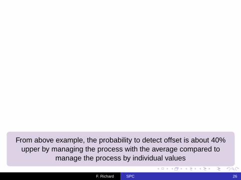
Probabilite : Definition n2

On se base sur la notion d’experience aleatoire (EA)EA repetable sous des conditions identiques (definition)⇒ On peut evaluer la frequence a laquelle l’evenement A se

realise en comptant le nombre de fois ou A s’est realise au termede n repetitions de l’experience aleatoireOn definit la frequence observee de A comme le rapport entre lenbre de realisation de A sur le nbre de repetitionsOn s’attend a ce que ces frequences observees different demoins en moins entre elles au fur et a mesure que le nombre derepetitions augmententOn peut definir une frequence theorique (probabilite)

P(A) = limn→∞f (A)

F. Richard SPC 52

Structure mathematique associee a la notion deprobabiliteAxiomatique de Kolmogorov

La probabilite associee a tout evenement est un nombre positifou nul et inferieur ou egal a 1

0 ≤ P(A) ≤ 1

La probabilite associee a l’ensemble des evenements d’uneexperience aleatoire est

P(Ω) = 1

Pour tout couple (A,B) d’evenement incompatible, la probabilitede la reunion de ces evenements est egale a la somme desprobabilite de A et B

P(A ∪ B) = P(A) + P(B)

F. Richard SPC 53

Structure mathematique associee a la notion deprobabilite

Axiomatique de Kolmogorov

Generalisation :

Si les evenements Aj (j denombrable) forment une suitedenombrable d’evenements incompatibles 2 a 2 :

P(∪jAj) =∑

j

P(Aj)

Experience aleatoire⇒ X : VA ∼ loi de probabilite

Exemple :

Lance de piece de monnaie (pile,face) : jeu de hasardX : pile, face ∼ loi de Bernouilli

F. Richard SPC 54

Structure mathematique associee a la notion deprobabilite

f (x) =

p si x = 1

1− p si x = 00 sinon

p : probabilite d’obtenir pile ou face

Si on lance n fois la piece (on realise n fois l’experiencealeatoire), on peut determiner la frequence de pile

fpile =

∑pilen P(x = pile) = limn→∞f (x = pile) = 0.5

Probabilite FrequenceExperience aleatoire Realisation d’expe. aleatoireVA Variable statistiqueLoi de probabilite Distribution statistiqueEsperence mathematique Moyenne arithmetiqueVariance Variance

F. Richard SPC 55

Theoreme central limite

”Toute somme (ou moyenne) de variables aleatoires independantesidentiquements distribuees (idd) tend vers une variable aleatoire

gaussienne(pour un nombre de VA tendant vers l’infini)”

”Independance”⇒ Les evenements aleatoires (ou VA) n’ont aucun influence l’un

sur l’autre

Exemple : lance de piece de monnaie. Le 1er lance n’a aucuneinfluence sur le 2eme lance

”Identiquement distribue”⇒ De meme loi parente

F. Richard SPC 56


Generalisation du theoreme central limite

Ce theoreme peut s’appliquer pour des VA independantes de loi deprobabilite differentes sous certaines conditions⇒ Conditions qui s’assurent qu’aucunes VA n’exercent 1

influence significativement plus importante (conditions de Lindeberget Lyapounov)

Exemple d’application du theoreme :

Experience aleatoire : trajet en voiture travail / domicile⇒ VA : X : tps de parcours, E(X ) = m, V (X ) = σ2

Realisation n fois de l’experience aleatoire⇒ nVA(X1,X2, ...Xn)

Yn =n∑

i=1

Xi ∼ N(nm;σ√

n) Yn =1n

n∑i=1

Xi ∼ N(

m;σ√n

)F. Richard SPC 57


X1,X2, ...,Xn independantes car de nombreux facteurs independantsentrainent la variation de la VA (meteo, feux rouges ...)

Application a la statistique mathematique

Experience aleatoire : Realisation d’1 piece mecanique⇒ VA : X : longueur de piece

Population (taille N)

IndividuX : loi de probabilité

2 paramètres : E(X)=m, V(X)=

Echantillon

(n-échantillon de taille n)

(X1,X2,...,Xn) n VA idd (vécteur aléatoire)

σ2

F. Richard SPC 58


Operateur, variation TC ... sont les facteurs independantsagissant sur la VA

Xn =1n

n∑i=1

Xi (moyenne d ′echantillonnage)

Xn ∼ N(

m,σ√n

)

F. Richard SPC 59

Loi normale

”La VA X suit une loi normale de parametres m (esperencemathematique) et σ2 (variance) si elle admet une densite de

probabilite f (x)”

f (x) =1

σ√

2πexp

[− 1

2

(x −mσ

)2]f(x)

x

X ∼ N(m, σ2)

Proprietes :

Loi symetriqueLoi ne dependant que de 2 parametres, m et σ

F. Richard SPC 60

Loi normale

f (x) =ddx

F (x) F (x) : fonction de repartition

F (x) = P(X ≤ x) =

∫ x

−∞f (x)dx

∫ +∞

−∞f (x)dx = 1

La fonction de repartition represente la probabilite que la VA Xait une valeur inferieure ou egale a une valeur x

F. Richard SPC 61

Loi normalef(x)

xF(x)

F(x)=1

x

1/σ√

2π

m − σ m m + σ

F (x) represente l’aire de la surfacesituee sous la courbe f (x) pour lesabscisses inferieures ou egale a x

Les points d’inflexion des 2 courbes se situent aux abscisses(m − σ) et (m + σ)

Le maximum de la courbe f (x) est de 1/σ√

2π et correspond aun abscisse de m

F. Richard SPC 62

Loi normale

L’ecart type σ a un effet ”concentrateur” de la courbe f (x)autour de m

E(X ) = m V (X ) = σ2 E(X ) = m = mode = mediane

Pour 1 variable continue :

E(X ) =

∫ +∞

−∞xf (x)dx

V (X ) =

∫ +∞

−∞

(x−E(x)

)2

f (x)dx

V (X ) = E[(

X−E(X )

)2]= E(X 2)−E(x)2 (formule de Konig)

F. Richard SPC 63

Loi normale

E(X n) =

∫ +∞

−∞xnf (x)dx (moment d ′ordre n)

E[(

X − E(X )

)n]=

∫ +∞

−∞

(x − E(x)

)n

f (x)dx

Criteres de normalite :

f(x)

x

99.74%

95%

68%

Abscisses exprimees enunite reduite (en nombred’ecarts types)

F. Richard SPC 64

Loi normale

Toutes les observations sont groupees autour de l’esperencemathematique de la facon suivante :

50% ∈ [m − 23σ; m + 2

3σ]

68% ∈ [m − σ; m + σ]

95% ∈ [m − 2σ; m + 2σ]

99.74% ∈ [m − 3σ; m + 3σ]

Demonstration

F. Richard SPC 65

Loi normale centree reduite

Exemple :

Etude de la repartition des notes a un exam des etudiants de L3(processus gaussien)⇒ Loi normale N(m, σ2)

On peut calculer m et σ car la population est de taille reduite

X =1n

∑Xi S2 =

1n

∑(Xi−X )2

f(x)

x

99.74%

xm-3S m+3S

F. Richard SPC 66


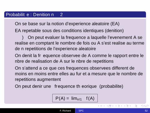
Le processus est gaussien, donc je peux verifier que 99.74% desnotes des etudiants se situent entre les valeurs (X − 3S) et (X + 3S)

Autre interpretation :

Si je prends au hasard un etudiant, j’ai 99.74% de chance que sanote se situe dans l’intervalle [X − 3S; X + 3S]

P(X−3S ≤ X ≤ X +3S) = 0.9974

2 cas possibles :

Je peux determiner 1 probabilite pour 1 intervalle donneJe peux determiner 1 intervalle pour une probabilite donnee

F. Richard SPC 67

Loi normale centree reduitef(x)

x

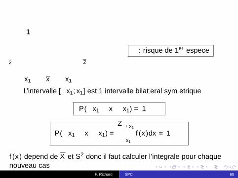
α : risque de 1er espece

1− α

α2

α2

−x1 x x1

L’intervalle [−x1; x1] est 1 intervalle bilateral symetrique

P(−x1 ≤ x ≤ x1) = 1− α

P(−x1 ≤ x ≤ x1) =

∫ +x1

−x1

f (x)dx = 1− α

f (x) depend de X et S2 donc il faut calculer l’integrale pour chaquenouveau cas

F. Richard SPC 68


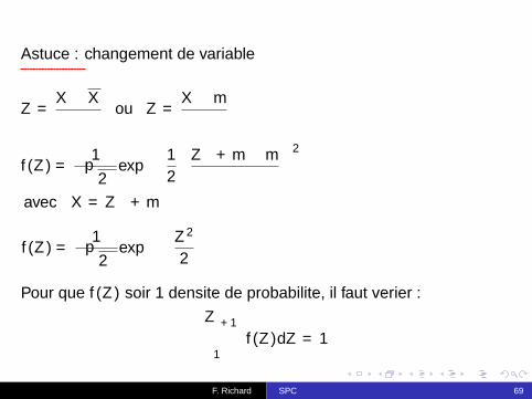
Astuce : changement de variable

Z =X − Xσ

ou Z =X −mσ

f (Z ) =1

σ√

2πexp

[−1

2

(Zσ + m −m

σ

)2]avec X = Zσ + m

f (Z ) =1

σ√

2πexp

[− Z 2

2

]Pour que f (Z ) soir 1 densite de probabilite, il faut verifier :∫ +∞

−∞f (Z )dZ = 1

F. Richard SPC 69

Loi normale centree reduite∫ +∞

−∞

1σ√

2πexp

[−Z 2

2

]=

1σ√

2π

∫ +∞

−∞exp

[− Z 2

2

]︸︷︷︸

integrale de gauss =√

2π∫ +∞

−∞f (Z )dZ =

1σ

On multiplie donc f (Z ) par σ pour verifier la relation :

∫ +∞

−∞f (Z )dZ = 1 ⇒ f (Z ) =

1√2π

exp[−Z 2

2

]On montre que :

E(Z ) = 0 V (Z = 1) Z ∼ N(0; 1) (loi normale centree reduite)

F. Richard SPC 70


Z =X −mσ

Z est 1 fonction pivotale car sa loi de probabilite N(0; 1) nedepend d’aucun parametres

f(z)

z

α2

α2

a b

P(a ≤ Z ≤ b) =

∫ b

af (Z )dZ = 1− α

∫ b

af (Z )dZ ⇒ table loi normale centree reduite

a et b dependent de αF. Richard SPC 71


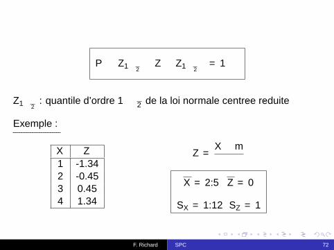
P(−Z1−α

2≤ Z ≤ Z1−α

2

)= 1−α

Z1−α2

: quantile d’ordre 1− α2 de la loi normale centree reduite

Exemple :

X Z1 -1.342 -0.453 0.454 1.34

Z =X −mσ

X = 2.5 Z = 0

SX = 1.12 SZ = 1

F. Richard SPC 72


X =14

(1 + 2 + 3 + 4

)= 2.5

SX =

√14

((1− 2.5)2 + (2− 2.5)2 + (3− 2.5)2 + (4− 2.5)2

)= 1.12

Z =14

(−1.34−0.45+1.34+0.45

)= 0

SX =

√14

((−1.34)2 + (−0.45)2 + (1.34)2 + (0.45)2

)= 1

F. Richard SPC 73

Intervalles de confiance

Soit 1 population de taille N :

On defini 1 VA X sur cette population ayant 1 loi de probabilitede parametres E(X ) = m et V (X ) = σ2

On defini 1 n-echantillon (X1,X2, ...,Xn), soit n VA idd

On defini 1 nouvelle VA, Xn : moyenne d’echantillonnage

Xn =1n

n∑i=1

Xi Xn ∼ N(m, σn) Xn ∼ N(

m,σ√n

)

Xn ∼ N(

m,σ√n

): distribution d’echantillonnage

F. Richard SPC 74


Si on s’interesse a la distribution statistique de la moyenne Xn detous les echantillons possibles de tailles n, cette distribution, appelee

distribution d’echantillonnage tend vers 1 loi normale N(m, σ√n )

1 objectif : Estimer m et σ (de la population)

Xn =1n

n∑i=1

Xi : estimateur sans biais de m

S2c =

1n − 1

n∑i=1

(Xi − Xn)2 : estimateur sans biais de m

F. Richard SPC 75


2 methodes d’estimation :

Estimation ponctuelleOn ne prend qu’un echantillon de taille n parmis tous lesechantillons possibles⇒ On introduit donc une ”erreur d’echantillonnage”

Estimation par intervalle de confiance

f(x)

x-x xx n

σn

Avec σn =σ√n

P(−X ≤ Xn ≤ X ) = 1−α

F. Richard SPC 76


∫ +x

−xf (x)dx = 1− α pour α fixe

f (x) depend de m et de σ ⇒ Changement de variable

Z =Xn −mσn

∼ N(0; 1) σn =σ√n

P(− Z1−α

2≤ Z ≤ Z1−α

2

)= 1− α

P(− Z1−α

2≤ Xn −m

σ

√n ≤ Z1−α

2

)= 1− α

P(

Xn−σ√n

Z1−α2≤ m ≤ Xn+

σ√n

Z1−α2

)= 1−α

F. Richard SPC 77


Si σ connu

P(

m ∈[Xn−

σ√n

Z1−α2

; Xn+σ√n

Z1−α2

])= 1−α

Si σ inconnu

T =Xn −mSn/√

n∼ T (n − 1)

La fonction pivotale T suit 1 loi de student a (n − 1) degre deliberte

S2n =

1n − 1

∑(Xi − Xn)2

F. Richard SPC 78


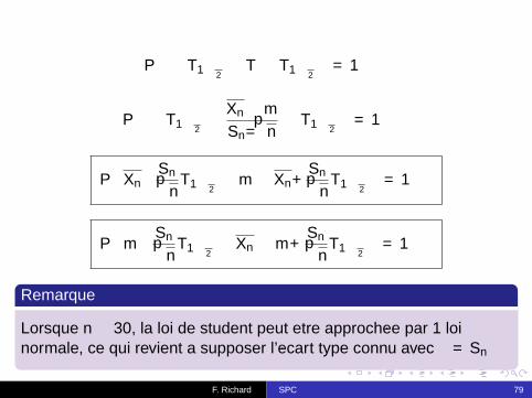
P(− T1−α

2≤ T ≤ T1−α

2

)= 1− α

P(− T1−α

2≤ Xn −m

Sn/√

n≤ T1−α

2

)= 1− α

P(

Xn−Sn√

nT1−α

2≤ m ≤ Xn+

Sn√n

T1−α2

)= 1−α

P(

m− Sn√n

T1−α2≤ Xn ≤ m+

Sn√n

T1−α2

)= 1−α

Remarque

Lorsque n ≥ 30, la loi de student peut etre approchee par 1 loinormale, ce qui revient a supposer l’ecart type connu avec σ = Sn

F. Richard SPC 79

Analogie avec les cartes de controle

L’objectif d’un processus c’est que sa population d’individus soitcentree sur la cible (cahier des charge)

m = cible

Xn represente donc la moyenne de la carateristique de qualitesur un echantillon de n individusClassiquement les limites de controle correspondent a l’intervalle

cible+−3σn

ce qui correspond implicitement a α = 0.0026

Les differentes constantes correspondent au terme suivant :

T1−α/2/√

n

F. Richard SPC 80

Efficacite d’une carte de controle

L’efficacite d’une carte de controle est l’efficacite a detecter undereglage

Il existe 2 risques decisionnel quant a la conclusion d’un dereglageou non

Le risque α (risque de 1er espece) de conclure a 1 dereglagealors qu’il n’y en a pas

Le risque β (risque de 2eme espece) de ne pas detecter 1dereglage alors qu’il y en a 1

F. Richard SPC 81


limite supérieure

de contrôle

limite inférieure

de contrôle

A B C

σσ√n

α2

α2

z1−α/2σ√n z1−α/2

σ√n

kσ

z1−α/2σ√n

β

zβ σ√n

F. Richard SPC 82


A : Valeur cible

B : Limite de controle (des moyennes)

C : Position du centrage du processus⇒ Le decentrage est de kσ

kσ = z1−α2

σ√n

+ zβσ√n

zβ = k√

n − z1−α2

C’est l’equation de la courbe d’efficacite

F. Richard SPC 83

Demonstration : E(X ) = m

f (x) =1

σ√

2πexp

[−1

2

(x −mσ

)2]

f ′(x) =

(1

σ√

2πexp

[−1

2

(x −mσ

)2])′

=1

σ√

2π

[−x −m

σ2 exp(−1

2

(x −mσ

)2)]

f ′(x) = −x −mσ2 f (x)

F. Richard SPC 84

Demonstration : E(X ) = m

E(X ) =

∫ +∞

−∞xf (x)dx ; posons x = σ2 x −m

σ2 +m

E(X ) =

∫ +∞

−∞

(σ2 x −m

σ2 +m)

f (x)dx

E(X ) = σ2∫ +∞

−∞

(x −mσ2

)f (x)dx︸︷︷︸

I1

+ m∫ +∞

−∞f (x)dx︸︷︷︸

I2

I1 = σ2∫ +∞

−∞−f ′(x)dx = −σ2

[f (x)

]+∞−∞

= −σ2[f (+∞)−f (−∞)

]= 0−0 = 0

I2 = m

F. Richard SPC 85

Demonstration : V (X ) = σ2

V (X ) = E(X 2)−E(X )2 = E(X 2)−m2

E(X 2) =

∫ +∞

−∞x2f (x)dx

Calculons E(X n) :

E(X n) =

∫ +∞

−∞xnf (x)dx

Posons :

x = σ2 x −mσ2 +m ; xn = x .xn−1

xn =

(σ2 x −m

σ2 + m)

xn−1

F. Richard SPC 86


E(X n) =

∫ +∞

−∞

(σ2 x −m

σ2 +m)

xn−1f (x)dx

=

∫ +∞

−∞σ2 x −m

σ2 xn−1f (x)dx︸︷︷︸I1

+

∫ +∞

−∞mxn−1f (x)dx︸︷︷︸

I2Calcul de I1 :

Rappel :∫ b

au′(x)v(x)dx =

[u(x)v(x)

]b

a−∫ b

au(x)v ′(x)dx

I1 = σ2∫ +∞

−∞xn−1︸︷︷︸

v

.

′x −mσ2 f (x)︸︷︷︸

u

dx

F. Richard SPC 87


v = xn−1 v ′ = (n − 1)xn−2

u′ = x−mσ2 f (x) = −f ′(x) u = −f (x)

I1 = σ2[−f (x)xn−1

]+∞−∞−σ2

∫ +∞

−∞(n−1)xn−2.−f (x)dx

= 0+σ2(n−1)

∫ +∞

−∞xn−2f (x)dx

= σ2(n − 1)E(X n−2)

I2 = mE(X n−1)

E(X n) = (n − 1)σ2E(X n−2) + mE(X n−1)

F. Richard SPC 88


V (X ) = E(X 2)−E(X )2 = E(X 2)−m2

E(X 2) = σ2E(X 0)+mE(X ) = σ2+m2

V (X ) = σ2

Retour

F. Richard SPC 89

Documents

Statistical Process Control - TuxFamilyfrichard.tuxfamily.org/wp-content/uploads/2018/03/spc.pdf”Statistical Process Control” F. Richard SPC 2. Introduction A process always ﬂuctuate,