www.elsevier.com/locate/ynimg

NeuroImage 22 (2004) 503–520

Statistical parametric mapping for event-related potentials (II):

a hierarchical temporal model

Stefan J. Kiebel* and Karl J. Friston

Functional Imaging Laboratory, Institute of Neurology, Wellcome Department of Imaging Neuroscience, London WC1N 3BG, UK

Received 16 October 2003; revised 7 February 2004; accepted 12 February 2004

In this paper, we describe a temporal model for event-related potentials

(ERP) in the context of statistical parametric mapping (SPM). In brief,

we project channel data onto a two-dimensional scalp surface or into

three-dimensional brain space using some appropriate inverse solution.

We then treat the spatiotemporal data in a mass-univariate fashion.

This implicitly factorises the model into spatial and temporal

components. The key contribution of this paper is the use of

observation models that afford an explicit distinction between

observation error and variation in the expression of ERPs. This

distinction is created by employing a two-level hierarchical model, in

which the first level models the ERP effects within-subject and trial

type, while the second models differences in ERP expression among

trial types and subjects. By bringing the analysis of ERP data into a

classical hierarchical (i.e., mixed effects) framework, many apparently

disparate approaches (e.g., conventional P300 analyses and time-

frequency analyses of stimulus-locked oscillations) can be reconciled

within the same estimation and inference procedure. Inference

proceeds in the normal way using t or F statistics to test for effects

that are localised in peristimulus time or in some time– frequency

window. The use of F statistics is an important generalisation of

classical approaches, because it allows one to test for effects that lie in a

multidimensional subspace (i.e., of unknown but constrained form). We

describe the analysis procedures, the underlying theory and compare

its performance to established techniques.

D 2004 Elsevier Inc. All rights reserved.

Keywords: Statistical parametric mapping; Event-related potentials;

Temporal model

Introduction

Electroencephalography (EEG) measures voltage changes on the

scalp induced by underlying neuronal activity. The EEG is thought

to be caused by postsynaptic potential changes in cortical pyramidal

neurons (Lopes da Silva and van Rotterdam, 1982). An important

1053-8119/$ - see front matter D 2004 Elsevier Inc. All rights reserved.

doi:10.1016/j.neuroimage.2004.02.013

* Corresponding author. Functional Imaging Laboratory, Institute of

Neurology, Wellcome Department of Imaging Neuroscience, 12 Queen

Square, London WC1N 3BG, UK. Fax: +44-20-7813-1420.

E-mail address: skiebel@fil.ion.ucl.ac.uk (S.J. Kiebel).

Available online on ScienceDirect (www.sciencedirect.com.)

application of EEG is to assess differences among responses to

different stimuli. Traditionally, one distinguishes between some

stimulus-locked component and a residual (error) process. The

stimulus-locked component is called the event-related potential

(ERP). Often, because of a low signal-to-noise ratio, one measures

several responses to estimate the average ERP, i.e., the common

component of all ERPs with respect to a given stimulus type.

In cognitive neuroscience, the analysis of multisubject-averaged

ERP data is well established. For example, guidelines for recording

standards and publication criteria are described in Picton et al.

(2000). In an ERP study, one analyses ERPs of several subjects

under several trial types (conditions). The analysis proceeds, at

each channel, by estimating a contrast or linear compound of the

ERP for each subject. Typically, these linear combinations are

averages over peristimulus time windows. The statistical test of

differences among these subject-specific, trial type-specific con-

trasts is based on an analysis of variance (ANOVA) with appro-

priate corrections for nonsphericity. This or a similar procedure

represents the conventional ERP analysis.

Another, more recent, analysis procedure is based on time–

frequency decomposition. Here, the hypotheses relate to power in

a specific frequency range within a peristimulus time window.

This kind of analysis is often used on single trial data to

characterise induced responses (non-time-locked), but can also

be applied to averaged ERP data (Tallon-Baudry et al., 1998). The

approach usually involves a continuous or discrete wavelet

transform. The wavelet transform has also been used to reduce

the ERP to one or a few wavelet parameters that capture,

parsimoniously, the differences among trial types or groups of

subjects. Some authors have used wavelet parameter estimates in a

descriptive fashion (Thakor et al., 1993) or have derived statistics

as the basis of inferences about ERP differences (Basar et al.,

1999; Trejo and Shensa, 1999).

Both the conventional and time–frequency analyses have been

used to detect and make classical inferences about differences,

between either trial types or groups of subjects. In this paper, we

show that both analyses can proceed within a unified statistical

framework using the same model. We propose a two-level hierar-

chical linear model as a general observation model for ERP data. In

this model, conventional and time–frequency hypotheses can be

tested using single- or multidimensional contrasts. The ensuing

statistics are either t- or F-distributed, where the degrees of freedom

S.J. Kiebel, K.J. Friston / NeuroImage 22 (2004) 503–520504

are adjusted for nonsphericity. As an alternative to t- or F-statistics

based on ordinary least squares, one can use the nonsphericity

estimate to whiten the data and derive maximum-likelihood esti-

mators. Inferences can be made at both levels of the model, resulting

either in a fixed effects or random effects analysis. In addition to

covering established characterisations, we will give examples of

other useful contrasts that arise naturally from our framework, that

do not conform to conventional or time–frequency analyses.

In the hierarchical model, the first level describes an obser-

vation model for multiple ERPs. The second level models the

first-level parameters over subjects and trial types. These contain

the differences or treatment effects one hopes to elicit by

experimental design. Critically, to derive valid statistics at the

second-level, one has to estimate the associated error covariance.

It transpires that one can choose the observation model, at the

first-level, to finesse nonsphericity estimation at the second. We

will illustrate this using a discrete wavelet transform at the first

level. The wavelet transform has two important features. The first

is that it decomposes the ERP in the time–frequency domain,

which gives a sparse representation of its salient features. The

second is that the wavelet transform affords an efficient error

Fig. 1. Example temporal matrices. (a) Full wavelet transform (Daubechies 4) in

Daubechies 4 set. We removed the two highest scales from the full wavelet transfo

matrix X (1) for two subjects with two conditions each.

covariance estimation at the second level. However, we stress that

other useful (linear) transforms like the Fourier transform can also

be used in the two-level approach. The approach described here

pertains to the analysis of single voxel data. We assume that the

error covariance matrix, at the second level, is known. In a

subsequent communication, we will describe the estimation

procedure in a mass-univariate setting (i.e., to spatially recon-

structed ERP data).

This paper comprises three sections. In the first, we describe the

mathematical basis of hierarchical models, paying special attention

to the formulation of conventional analyses within this framework.

In the second section, we provide worked examples using simu-

lated and real data to demonstrate the use and flexibility of our

approach. We conclude with a discussion of how this procedure

relates to other analyses in the literature.

Hierarchical models

This section establishes the temporal model that is used, in

various forms, in the next section. This is a two-level hierarchical

design matrix form. (b) Truncated wavelet matrix X t generated using the

rm giving 64 wavelet regressors out of a potential 256. (c) First-level design

Fig. 2. Example of first-level covariance components Qk(1). We modelled

four ERPs (from an experiment with two subjects with two trial types each).

Each component models the variance of a single ERP.

S.J. Kiebel, K.J. Friston / NeuroImage 22 (2004) 503–520 505

model (where we estimate model parameters in a two-stage

procedure, see below).

The model is

y ¼ X ð1Þbð1Þ þ �ð1Þ

bð1Þ ¼ X ð2Þbð2Þ þ �ð2Þ ð1Þ

where y is the data vector, X (1) and X (2) are design matrices, b (1)

and b(2) are parameter vectors, and �(1) and �(2) are normally

distributed error vectors. The data y comprises stacked ERPs yij,

where i = 1,. . ., Nsubjects, j = 1,. . .,Ntypes. Nsubjects is the number of

subjects and Ntypes is the number of trial types.

First-level model specification

The model at the first level is described by the design matrix

X ð1Þ ¼ INsubjectsNtypes� X t ð2Þ

and the error covariance matrix

Cð1Þ ¼ diagðkð1ÞÞ � Ct ð3Þ

where X t is the Nbins � Np matrix that models the temporal

components of a single ERP. The operator diag(�) returns a matrix

with the vector argument on its main diagonal and zeros elsewhere.

The observation error covariance matrix C (1) can be decomposed

into ERP-specific components weighted by variance parameters

kk(1), where k = 1,. . .,NsubjectsNtypes (see below).

The matrix X t can represent any linear transform of the ERPs.

Here, we consider a wavelet transform. The wavelet transform

enables the decomposition of the data into time–frequency com-

ponents. An excellent and intuitive introduction to the wavelet

transform can be found in Gershenfeld (1998). A more rigorous

treatment is provided by Strang and Nguyen (1996). In our

implementation, we use an explicit matrix representation, which

is a sequence of multiplications of filter and permutation matrices

(Gershenfeld, 1998; Press et al., 1992). The matrix representation

allows us to formulate the wavelet model as a design matrix.

Moreover, as illustrated by the SPM package for the analysis of

functional magnetic resonance imaging (fMRI) data, the design

matrix can be portrayed as an image to provide an intuitive

understanding of the model.

In this paper, we use the Daubechies wavelets of order 4

(Daub4) (Daubechies, 1992). This wavelet transform is one of the

more commonly used in the literature. The Daub4 transform is an

orthogonal wavelet transform with compact support. The implicit

transform is framed in terms of parameter estimation within the

hierarchical model. An example of the temporal matrix X t and an

associated first-level design matrix is shown in Fig. 1.

If X (1) is square, i.e., if we use a nontruncated wavelet transform,

the covariance matrix of �(1), C (1), cannot be estimated and Eq. (1)

ceases to be an observation model. Otherwise, if Np < Nbins, �(1) is

assumed to be normally distributed with �(1) f N(0,C (1)).

The matrix C (1) can be decomposed into between-ERP compo-

nents (e.g., different levels of observation noise denoted by kk(1)) and

the within-ERP component C t (Eq. (3)). For simplicity, we will

assume homogeneous variance over peristimulus time and within

subject with zero covariances; that is, the measurement error in each

ERP is assumed to be white noise with ERP-specific variance so that

C t = INbins. This white-noise assumption can be motivated by

assuming that the physiologically mediated within-ERP noise is

dominated by the measurement noise. In our model, random

physiological effects reside in �(2) (see below and Summary and

discussion). This gives us components Qkt , k = 1,. . .,NsubjectsNtypes

(c.f. companion paper, Eqs. (3) and (4)). These are ordered in a block

diagonal fashion so that

Cð1Þ ¼X

k

kð1Þk Qtk ð4Þ

¼ diagðkð1ÞÞ � INbinsð5Þ

¼ diagðkð1ÞÞ � Ct ð6Þ

An example of first-level covariance components is shown in Fig. 2.

The vector k(1) has lengthNsubjectsNtypes and consists of the first-level

variance parameters k(1) = k1(1),. . .,k(1)NsubjectsNtypes

. This means that the

observation noise variance can be different for each subject and

condition.

Second-level model specification

The second-level design matrix X (2) models the first-level

parameters over subjects,

X ð2Þ ¼ X d � INpð7Þ

and

Cð2Þ ¼XN dcomp

l

XNpcomp

m

kð2Þlm ðQdl � Qp

mÞ ð8Þ

where the experimental design matrix X d encodes subject- and trial-

type-specific treatment effects. The second-level error covariance

S.J. Kiebel, K.J. Friston / Neuro506

matrix C (2) is modelled using a linear mixture of covariance

components. As for the design matrix X (2), C (2) can be decomposed

into design-specific components Q d (e.g., within-subject correla-

tions) and physiological error Qp. Although this (physiological)

random effect is treated as ‘error’, from the point of view of the

statistical model, it could well represent highly structured variation

in event-related processes. The error sources are modelled using

Ncompd Ncomp

p components. These components are weighted by var-

iance parameters klm(2) .

Using X d to generate the second-level design matrix provides a

general approach that can embrace many different experimental

designs, e.g., modelling condition-specific effects or group compar-

isons. An example of X (2) based on X d = 1Nsubjects� INtypes

(a simple

averaging matrix that averages over subjects across trial types) is

shown in Fig. 3. (1N denotes a column vector of ones of length N).

The physiological error components Qmp are generally nonspher-

ical, even with the reparameterisation implicit in wavelet trans-

forms, because of intersubject variation in the way ERPs are

expressed. A prominent feature of intersubject error is that its

variance changes with peristimulus time. For example, at presti-

mulus time points, low error variances prevail, whereas the

variance increases around phasic components like the N1 and then

decreases again. This sort of nonsphericity is probably due to

latency variations and other mechanisms that shape neuronal

transients. Any model, for the second-level error, needs to capture

this nonstationary variance and attending correlation structure. This

is not a simple task, because one does not usually have enough

observations to estimate a highly parameterised model of the error

at a single voxel. There are two principled approaches to this

covariance component estimation issue. The first is to use prior

knowledge about the ERPs’ structure to reduce the number of first-

level parameters and associated covariance parameters at the

second level. The second is to compute precise empirical estimates

using data from other voxels. In this paper, we assume that we

know the structure of the error covariance matrix at the second

level, C(2), and defer the description of its estimation for spatially

extended ERP data, using the second approach, to a subsequent

communication.

Fig. 3. Example of second-level design matrix X (2) for two subjects with

two trial types. This design matrix models the trial type-specific averages.

At the first level, each trial type is modelled using Np = 64 wavelet

regressors.

Hierarchies and empirical Bayes

An important aspect of hierarchical observation models is that

they lend themselves to an empirical Bayesian interpretation. In

the current model, the second-level error matrix C(2) is equivalent

to the prior covariance of the parameters b(1) at the first level

(Friston et al., 2002), i.e.

Cð2Þ ¼ Covð�ð2ÞÞ ¼ Covðbð1ÞÞ ð9Þ

This means C (2) can be regarded as describing intersubject

variability, or as placing prior constraints on the subject-specific

estimate of b (1). Although not pursued here, this perspective on

C (2) leads to a parametric empirical Bayes approach in which C (2)

can be used as a shrinkage prior on conditional estimates of b (1).

See Friston et al. (2002) for details. In this paper, we are interested

in estimating b (2) as opposed to b (1). Because there are no priors

on the second-level parameters, conditional and maximum-likeli-

hood estimates reduce to the same thing and the empirical Bayes

perspective can be discounted. However, the notion of treating

C (2) as a prior covariance has implications for the choice of X t. We

will return to this in the discussion.

Estimation

After model specification (Eqs. (1)– (8)), we estimate the

parameters using maximum likelihood (ML) or ordinary least

squares (OLS). Variance parameter estimates are obtained using

restricted maximum likelihood (ReML). To render the method

computationally efficient, a two-stage procedure can be used

(Holmes and Friston, 1998): This entails (i) estimating the first-

level parameters for each subject and trial type and taking the

ensuing estimates b (1) to the second level. (ii) At the second level,

we compute ML or OLS estimates of b (2) and ReML estimates of

k(2). We can do this in two distinct stages because X t (Eq. (2)) is the

same for all subjects and trial types. For ML estimators at the

second level, we would require kk1(1) c kk2

(1) for any pair of ERPs k1and k2 (Eq. (4)). When modelling inhomogeneous variances over

subjects, at the first level, the two-stage procedure remains valid but

the ensuing generalised least-squares estimators are no longer ML.

However, we expect that the deviation from the ML estimates is

small compared to the typically observed between-subject variabil-

ity at the second level. In this paper, we use OLS estimates to enable

a more direct comparison with conventional approaches. However,

in practice, ML estimates are preferable, because they are more

precise and lead to more sensitive inferences.

Inference—contrasts

After parameter estimation, the next step is to make inferences

about specific effects. In a classical setting, this proceeds using

contrast vectors (or matrices) that specify null hypotheses (H0).

After parameter estimation, we derive a statistic that tests H0. If the

associated P value is small enough, one can reject H0. In this

section, we describe the generation and use of contrasts. In the next

section, we will deal with statistical inference, i.e., the estimation

of the P value associated with the contrast.

An introduction to contrasts in the context of linear models is

given in Poline et al. (2004). A contrast is a linear combination of

parameter estimates that defines a specific null hypothesis about

the parameters. Within our model, the parameters are wavelet

Image 22 (2004) 503–520

S.J. Kiebel, K.J. Friston / NeuroImage 22 (2004) 503–520 507

coefficients. However, it is not always intuitively obvious how null

hypotheses can be specified in wavelet space. This problem can be

solved by formulating contrast weights in peristimulus time or in

the (peristimulus) time–frequency domain and projecting them to

the second level.

Generation of second-level contrast vectors

Because we are dealing with a hierarchical observation model,

the contrast vector factorises into two terms c(2) = cd � cw. The

vector cd prescribes the comparison at the level of the experimental

design (e.g., [�1 1]T to compare the two trial types in the examples

above). This component specifies which ERPs should be tested.

The second component cw specifies what aspect of the ERP we are

interested in. This is usually some ERP component that is restricted

Fig. 4. Creating contrasts at the second level, where the hypothesis is specified ov

terms of design; right: hypothesis in terms of what ERP features exhibit the desi

in time–frequency. The simplest example would be a peristimulus

time window defined by a vector w with wi = 1 within the window

and wi = 0 elsewhere. The within-ERP contrast weights cw are

defined by w through

cwT ¼ w�X t

cð2Þ ¼ cd � cw ð10Þ

where w� is the generalised inverse of w. For a simple time

window, w�yi is the average of the ith ERP in the window

(Fig. 4). More generally, w will be a matrix spanning a subspace

of Xt that is restricted to a time–frequency window.

The contrast c(2)T

b(2) can then be tested in the usual way by

forming t- or F-statistics (see next subsection). This projection

procedure is general in the sense that it factorises the second-level

er two subjects with two ERPs each (window averages). Left: hypothesis in

gn effect.

Fig. 5. Example of a two-dimensional contrast component, see text for description. Left: hypothesis w in measurement space; right: contrast component cw in

wavelet space.

S.J. Kiebel, K.J. Friston / NeuroImage 22 (2004) 503–520508

contrast vector c(2) into two components cd and cw. A change in the

question at either the design level or at the level of the ERP can

then be implemented by changing a single component. For

example, more elaborate hypotheses like interactions in factorial

designs can be specified by adjusting cd. To test other time–

frequency windows, one only needs to change cw.

Note that, throughout the paper, our working assumption is

that the basis set X t captures most of the interesting variability

in ERP data. This is true for the basis sets and the data

analysed in this paper. However, if X t misses too much of the

experimentally induced variance, contrasts at the second level

become difficult to interpret, because their projection back onto

measurement space may not conform to what was required

(i.e., w p X tX t�w).

Second-level contrast matrices

Specifying hypotheses in this way can be generalised in a useful

and powerful way by allowing w to be a Nbins � Ncon matrix. This

leads to multidimensional second-level contrasts. For example, in

Fig. 6. Example of a two-dimensional time–frequency wmatrix. Top: matrix w in m

fMRI, contrast matrices are useful when testing for responses

mediated by haemodynamic response functions (HRF) of unknown

form. In this case, the haemodynamic response function is mod-

elled by basis functions (the principal response shape and two first

partial derivatives; Friston, 2002). One can then form a three-

column contrast matrix that tests for any effect spanned by

regressors formed from the three basis functions.

For ERP data, the same principle can be used to test for effects

that are modelled by multiple columns in w. A simple example,

which builds upon the window averaging approach described

above, is to test for effects distributed over multiple windows. In

the simplest case, instead of testing for a single window, we can

test for any effect in two or more neighbouring time windows.

Fig. 5 shows two columns of the resulting matrix w.

Importantly, this approach allows for a large range of tests in the

time–frequency domain. Contrast matrices are particularly useful

for testing frequency-specific subspaces. Suppose we want to test

for the expression of power at a given frequency in a particular

peristimulus time window. This can be achieved by using a matrix

w with two columns that comprises two modulated sinusoids with

easurement space for a single ERP. Bottom: associated cw in wavelet space.

S.J. Kiebel, K.J. Friston / NeuroImage 22 (2004) 503–520 509

p/2 relative phase. The modulation can be any window function

(e.g., a Gaussian) centered on the peristimulus time of interest. Such

a time–frequency contrast matrix is shown in Fig. 6.

The notion of factorising hypothesis specification into a design

component and an ERP component is at the heart of the generalisa-

tion of classical approaches proposed in this paper. Normally, in

conventional analysis, the ERP component is completely predeter-

mined by the window averaging applied to the data. In our

application, this averaging represents one of many hypotheses that

could have been tested, possibly jointly, and is specified through the

second-level contrast. Operationally, this means the user has to

specify the design contrast and the ERP contrast separately, the

latter in observation space. A potentially useful and flexible way of

specifying the ERP component is in terms of a time–frequency

Fig. 7. Creating time–frequency contrast matrices at the second level, where the

hypothesis in terms of design, i.e., the average over two trial types; right: hypothe

any activity around time bin 50, in the frequency band between 1 and 28 Hz. Eight

used to generate the second-level contrast matrix c(2).

window (see Fig. 7). This allows the user to test for any response that

lies within certain peristimulus time and frequency bounds. A

temporally long, frequency-restricted window would implicitly test

for stimulus-locked transients in a prespecified frequency band. In

contradistinction, a short window, covering multiple frequencies,

would test for a temporally localised shape of unspecified form or

frequency.

Critically, in the limiting case that the window includes only the

lowest frequency (i.e., constant term), the resulting contrast is one-

dimensional and conforms to the temporal window. This is exactly

the same as the classical time-window averaging approach. In

short, multidimensional contrasts admit hypotheses about time–

frequency effects that subsume the classical testing procedure. This

is illustrated graphically in Fig. 7, which should be compared to

hypothesis is specified as a rectangle in the time– frequency domain. Left:

sis in the ERP time–frequency domain. The hypothesis is whether there is

contrast vectors cw are left after orthogonalisation (see text). These are then

S.J. Kiebel, K.J. Friston / NeuroImage 22 (2004) 503–520510

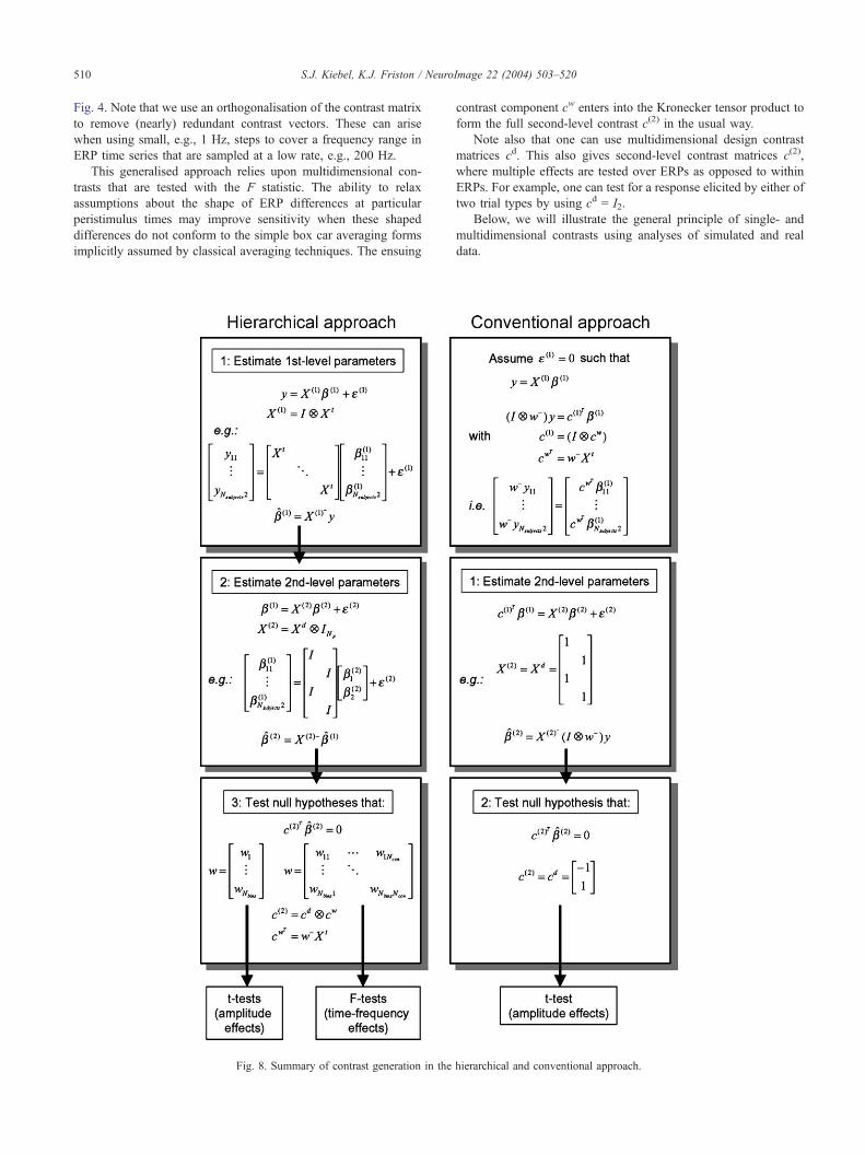
Fig. 4. Note that we use an orthogonalisation of the contrast matrix

to remove (nearly) redundant contrast vectors. These can arise

when using small, e.g., 1 Hz, steps to cover a frequency range in

ERP time series that are sampled at a low rate, e.g., 200 Hz.

This generalised approach relies upon multidimensional con-

trasts that are tested with the F statistic. The ability to relax

assumptions about the shape of ERP differences at particular

peristimulus times may improve sensitivity when these shaped

differences do not conform to the simple box car averaging forms

implicitly assumed by classical averaging techniques. The ensuing

Fig. 8. Summary of contrast generation in the

contrast component cw enters into the Kronecker tensor product to

form the full second-level contrast c(2) in the usual way.

Note also that one can use multidimensional design contrast

matrices cd. This also gives second-level contrast matrices c(2),

where multiple effects are tested over ERPs as opposed to within

ERPs. For example, one can test for a response elicited by either of

two trial types by using cd = I2.

Below, we will illustrate the general principle of single- and

multidimensional contrasts using analyses of simulated and real

data.

hierarchical and conventional approach.

Fig. 9. Real and simulated ERPs. Left: 16 randomly chosen ERPs out of 54 at channel PO8. Right: 16 simulated ERPs generated by using a covariance matrix

S.J. Kiebel, K.J. Friston / NeuroImage 22 (2004) 503–520 511

Inference—statistics

Having specified second-level contrasts, we can make infer-

ences using the estimated parameters. Note that a second-level

contrast specifies a random effects analysis. In this subsection, we

describe the formation of t and F statistics to test null hypotheses

about these contrasts.

The t statistic is given by

t ¼ cð2ÞT

bð2Þ

ˆStdðcð2ÞT bð2ÞÞð11Þ

where c(2) is a second-level contrast vector and ˆStd denotes the

estimated standard deviation. The parameters can be estimated

using generalised least squares to give ML estimators. Their

standard deviation is estimated in the usual way using ReML

based on real data (see text).

Fig. 10. Comparison of P values on null data using a conventional and

hierarchical model. The inter-ERP variability of the synthetic data was

derived from real data (see text). Results are displayed on a log– log scale.

Dashed line: P values required for an exact test, Dotted line: conventional

analysis. Solid line: hierarchical model.

variance component estimators (Friston et al., 2002). However,

because this paper uses OLS estimators, we are obliged to use a

Satterthwaite approximation to compute effective degrees of free-

dom (Worsley and Friston, 1995; Kiebel et al., 2003). P values can

then be computed using the cumulative density function (CDF) of

the null distribution of the sampled t value.

When using a contrast matrix (or vector), one implicitly defines

a reduced model. In the context of nested models, the F statistic is

used to compare the corresponding sum of squares:

F ¼ bð1ÞTM bð1Þ

bð1ÞT Rbð1Þm2m1

fFm1;m2 ð12Þ

where M = R0 � R, R = I � X (2)X (2)� is the residual forming

matrix of the full model. Matrix R0 is the residual forming matrix

of the reduced model, where R0 = X(2)c0(2) and c0

(2) = I � c(2)c(2)�I.

The degrees of freedom m1 and m2 are estimated using a Sat-

terthwaite approximation. P values can be derived from the CDF of

the null distribution of F.1

In summary, this section has described how to formulate a two-

level hierarchical model with multiple covariance components,

estimate model parameters, specify contrasts and estimate P

values. In the following, we will deal with the conventional model

for ERP data. This model is a special, if trivial, case of the

hierarchical two-level model. We will then compare conventional

and hierarchical analysis procedures using simulated and real ERP

data.

The conventional model

In classical ERP research, one assumes that each single trial

comprises the ERP and some (usually white) normally distributed

measurement noise. Under these assumptions, a natural estimator

for the ERP of subject i and trial type j, yij, is the average of all

single trials yijn, n = 1,. . .,Ntrials, i.e., yij = 1/Ntrials S1Ntrialsyijn. Given

ERP estimates for each subject i and each trial type j, one then

computes contrasts w�yij, e.g., the average over a peristimulus time

window. These contrasts then enter an analysis of variance

(ANOVA). The ensuing nonsphericity, i.e., inequality of variances

1 The square of the t statistic is an F statistic. Therefore, in SPM, the t

statistic provides for one-tailed tests only.

Fig. 12. Comparison of P values on synthetic data using a conventional and

two-level model. The data was generated as described in the text. The data

contained ERP differences (an N170 component as shown in Fig. 11),

which we tested for. Dashed line: P values under null hypothesis. Dotted

line: conventional model. Solid line: two-level model.

S.J. Kiebel, K.J. Friston / NeuroImage 22 (2004) 503–520512

of each trial type or covariance between them, is usually accom-

modated using a Greenhouse–Geisser correction. This correction

approximates the null distribution of the F statistic by adjusting the

effective degrees of freedom. An example of such an analysis can

be found in Henson et al. (2003) and is the quasi standard in the

experimental ERP literature.

It is useful to formulate the conventional approach in terms of

the two-level model. We can implement averaging over a peristi-

mulus time window for all subjects and trial types as a contrast

matrix c(1) = INsubjectsNtypes� w�T. As above, wi = 1 for peristimulus

times in the window and wi = 0 at all other times. The implicit

model can be expressed mathematically as

y ¼ X ð1Þbð1Þ

¼ bð1Þ

cð1ÞT

bð1Þ ¼ X ð2Þbð2Þ þ �ð2Þ ð13Þ

where X (1) is the identity matrix and X (2) = X d � I1 = X d. As

above (Eq. (7)) the matrix X d encodes experimental design

variables. The amplitude difference between trial types is assessed

using a second-level contrast c(2) = cd = [�1 1]T. Note here that

there is no partitioning of the response into the observation noise

and the physiological ERP variability. This means the conventional

model assumes �(1) = 0 and the two-level model reduces to a one-

level model.

This is the first key difference between the conventional and

the hierarchical model. The second is that the conventional

model only passes a single contrast per ERP to the second level.

This means that, in the conventional model, each hypothesis test

is based on a separate model specification and estimation pro-

cedure. In contrast, the hierarchical model parameters are only

estimated once. A family of hypotheses can then be tested at the

second level without model refitting. The conventional approach

precludes this because only contrasts of first-level parameters are

taken to the second level. As will be illustrated in the next

section, the two-level model enables us to test hypotheses that

could never be tested in a conventional analysis. Furthermore,

the conventional approach precludes hypothesis tests for treat-

Fig. 11. Signal component used for simulations. This component is the

fourth eigenvector of the sample data covariance matrix of 54 ERPs.

ment effects that span several dimensions (e.g., time–frequency

analyses).

The fundamental differences between the hierarchical and

nonhierarchical (i.e., conventional) procedures are summarised in

Fig. 8.

Illustrative analyses

In this section, we apply the hierarchical and conventional

methods to synthetic and real data. The synthetic data were

designed to show that the hierarchical approach gives valid tests

and retains sensitivity. Furthermore, we will demonstrate contrasts

that can only be used in a hierarchical context. Analyses of real

data are provided to illustrate the operational details, particularly

contrast specification.

Synthetic data

Synthetic data were constructed by sampling ERPs from a

normal distribution whose moments were based on real ERP data.

We selected a channel, PO8, which showed a N170 component in

response to face stimuli (Henson et al., 2003). We used 18 subjects

with three trial types giving 54 ERPs of length 256 sampled at 200

Hz. We computed the grand mean ERP and the singular value

decomposition (SVD) of the sample residual covariance matrix.

ERP data were simulated by drawing from the empirically defined

multivariate Gaussian distribution with the sampled ERP mean.

The covariance was computed using only the first 15 eigenvectors

of the sampled covariance matrix. This corresponds to components

Qp in Eq. (8). The restriction to the principal components of ERP

variability biased the nonspherical variation, in simulated data,

towards physiological as opposed to measurement sources of

variance. In Fig. 9, we compare 16 randomly selected ERPs with

Fig. 13. Time– frequency two-column contrast matrix to test for evoked power, at 40 Hz, averaged over two trial types. The modulating Gaussian is centered at

stimulus onset and has a FWHM of 75 ms.

2 We used a precise estimate based on data from all channels.

S.J. Kiebel, K.J. Friston / NeuroImage 22 (2004) 503–520 513

16 simulated ERPs. One can see clearly that the simulated data

show many features of real ERPs. More importantly, the residual

covariance structure of the simulated data is roughly the same as of

real ERPs (not shown).

In the following, we use these data for assessing the speci-

ficity and sensitivity of our approach in relation to conventional

analyses.

Each synthetic epoch consisted of 256 time points. Each

simulation comprised six subjects with two trial types each giving

12 single-channel ERPs. For each set of simulations, we generated

104 data sets. In the first two simulations, we assess specificity and

establish that the hierarchical and conventional approaches are

valid. In the second set of simulations, we show that our approach

is sensitive to a differential signal typically tested for by conven-

tional analyses. In the third set of simulations, we use multidimen-

sional contrasts to test for evoked power, in a time–frequency

window, over two trial types. In the final set of simulations, we

illustrate how one can use a two-dimensional contrast to test for

biphasic signals.

Specificity

In the first set of simulations, we generated synthetic data as

described above. We tested for a difference in ERP amplitude over

150–190 ms between the two trial types, over six subjects (note

that this difference has zero expectation in the simulated data, i.e.,

there is no differential ERP signal). This peristimulus time window

contains the N170 component (see also Fig. 17). As described

above, the N170 hypothesis can be specified in measurement space

by a vector w = 1 within the peristimulus time window and w = 0 at

other times.

For the conventional analysis, we computed 12 ERP-specific

first-level contrasts c(1)Ty, where c(1) = I12 � w�. The second-level

design matrix X(2) = X d = 1Nsubjects� I2 implemented a simple

averaging over subjects enabling a two-sample t test. We tested for

an amplitude difference between the trial types using the second-

level contrast vector [�1 1]T.

For the hierarchical approach, we used, at the first level, a full

(eight scales) wavelet decomposition (Daubechies 4) and removed

the two highest scales. This implements a truncation based on the

prior assumption that the signal subspace does not span the highest

two scales. All first-level parameter estimates b(1) were brought to

the second level. The second-level contrast vector was [�1 1]T� cw

(Eq. (10)).

We modelled the observation error (Eq. (4)) as homogeneous

over the six subjects. At the second level, we assumed the error

covariance matrix to be known.2

The results of the simulations are shown in Fig. 10 as a P–P

plot. In this plot, lines above the identity represent invalid, or

capricious performance, regions below the identity represent con-

servative performance. Both methods returned P values that are

very close to the distribution necessary for an exact and valid test.

Sensitivity

In the second set of simulations, we generated synthetic data

using the procedure described above. However, we added a

differential signal to the ERPs of the second trial type. This signal

conformed to a N170 component. The shape of the signal was

taken from the fourth eigenvector of the sample data covariance

matrix. This eigenvector captured the form of the N170 component

(Fig. 11). In all simulations, we added this signal to the simulated

ERPs of one trial type so that we generated a differential signal

Fig. 14. Distribution of P values for null data testing for power at 40 Hz

averaged over two trial types. The data was generated as described in the

text. Results are displayed on a log– log plot. Dashed line: P values

required for an exact test. Solid line: two-level model.

S.J. Kiebel, K.J. Friston / Neuro514

between trial types. The amplitude of this signal was 40% of the

estimated average amplitude of the N170. We used the same model

and contrasts as in the first set of simulations; that is, we tested for

a difference in amplitude between trial types in the 150–190 ms

time window. In Fig. 12, the P–P plot shows that both approaches

give roughly the same sensitivity to this signal. The hierarchical

approach seems to result in slightly more sensitive results, but this

might be due to the Satterthwaite approximation for a single

variance parameter (Kiebel et al., 2003).

Fig. 15. Contrast generating vectors in measurement space. These vectors are used

or 170 ms.

Contrast matrices and time–frequency contrasts

In these simulations, we illustrate hypothesis testing in the

time–frequency domain. We asked whether the power, of evoked

oscillations at 40 Hz, averaged over two trial types, in a given

peristimulus time window is greater than chance expectation. To

generate second-level contrasts, we specified matrix w (Eq. (10)) as

two modulated sinusoids in measurement space (cf. Fig. 6). Both

sinusoids had a frequency of 40 Hz, where one was phase shifted by

p/2. The sinusoids were windowed with a Gaussian centered at 0 ms

in peristimulus time, i.e. at stimulus onset, with a full width at half

maximum (FWHM) of 75 ms. This hypothesis was chosen, because

we wish to assess the specificity of the resulting test (see below). To

average over trial types, we used cd = [1 1]T (Eq. (10)). The ensuing

columns of c(2) = cd � cw are shown in Fig. 13. This way of testing

for evoked oscillations is quite general and can be extended to test

not only a specific frequency, but frequency ranges by using pairs of

windowed sinusoids to cover the frequencies required (Fig. 7).

We used simulated data to assess the specificity of inferences

using the F statistic (Eq. (12)). To ensure the data conformed to the

null hypothesis, we sampled simulated data, for this set of

simulations only, from a multivariate normal distribution with zero

mean. The results are shown in Fig. 14 and indicate valid and exact

tests. This example demonstrates the utility of the two-level model

because this analysis is precluded by the conventional approach

(i.e., there is no single contrast vector c(1) that can be used to test

for evoked oscillations of unknown phase).

In this subsection we have introduced the use of multidimen-

sional contrasts to test for evoked frequency-specific oscillations at

a particular peristimulus time. In applying this contrast to null data

(no average ERP difference), we hope to have established its

validity by showing the false-positive rate conforms to its nominal

value. In a later section, we will use a similar contrast to test a

time–frequency hypothesis in real data that did evidence signifi-

cant power in the alpha band.

Image 22 (2004) 503–520

to test for a difference between trial types in either a component around 100

Fig. 16. Distribution of P values when testing for a biphasic signal with the

conventional and the two-level model. With the conventional model, we

used three different contrasts to show that one cannot completely capture the

biphasic signal with a single contrast vector. Dashed line: P values under the

null hypothesis. Green line: two-level model. The other lines show the P

values from the conventional model testing for a change in component 1

(red), in component 2 (blue), and a change in their average (magenta).

S.J. Kiebel, K.J. Friston / NeuroImage 22 (2004) 503–520 515

Other multidimensional contrasts

In this last set of simulations, we illustrate another application

that is precluded by the conventional approach. We test for the

difference, in a compound signal, between two trial types. The

signal of interest consists of two components, the first (early)

centered around 100 ms, the second (late) around 170 ms. The

difference (between trial types) could be expressed in either or both

components. In this case, a single contrast vector will not be

optimally sensitive, because we have no prior knowledge about the

relative contribution of the two component differences. Differences

of unknown form like these can be assessed using a two-column

Fig. 17. Preprocessed single-channel ERP data as a function of peristimulus

time. Blue: ERPs of trial type 1 (unfamiliar faces); red: ERPs of trial type 2

(scrambled faces).

contrast matrix cw. Each column supports one of the components in

peristimulus time. In measurement space, we can specify each

component in terms of a standard averaging window, or some other

user-specified shape. Here, we chose a Gaussian form for

w (Fig. 15). The test for any difference in the amplitudes of the

Gaussians is implemented by defining cd = [�1 1]T and computing

the second-level contrast c(2) = cd � cw. This principle can be

generalised to more components by adding more Gaussians to the

matrix w. The F statistic provides an overall test for any difference

expressed over the components of w. The nature and form of any

significant difference is characterised by the contrast of parameter

estimates.

We generated synthetic data using the procedure described

above. We added differential signal that consisted of a biphasic

signal (a mixture of two Gaussians). The amplitudes of the two

Gaussians were drawn independently from a Gaussian distribution

with zero mean and variance 4. The signal to noise ratio (SNR) is

0.47 (c.f. Fig. 17).

In Fig. 16, we show the results of the simulations. For each of

the 104 data sets, we tested the hypothesis of any difference, in

either component, using the F statistic (Eq. (12)). For the conven-

tional approach, we used three different single-dimensional con-

trasts for a two-tailed test based on the F statistic. Two of these

tested for a difference in a single component, and the third tested

for a mean difference over both components. These tests show the

sensitivity one can hope for with the conventional approach. The

hierarchical model with a two-dimensional contrast leads to a test

that is at least as sensitive as the most sensitive test based on the

conventional model. This is because the alternative hypothesis

spans both dimensions of the real treatment effect.

Applications to real ERP data

Here, we describe an analysis of (real) ERP time series using

the conventional and hierarchical models. The hypotheses tested

below were chosen because they illustrate many of the procedural

details and concepts of the two-level approach.

The data were acquired during a memory study, which involved

the presentation of faces and scrambled faces to 18 subjects

(Henson et al., 2003).

Fig. 19. Time– frequency representation of the averaged power of

multisubject ERP data at channel PO8 between 6 and 20 Hz over

peristimulus time.

Fig. 18. Fitted back-projected data, in measurement space, from the conventional and hierarchical model. (Left) Conventional model; (right) two-level model.

o-level model shows a jagged shape because of the truncated wavelet transform.

S.J. Kiebel, K.J. Friston / NeuroImage 22 (2004) 503–520516

An ERP analysis

The EEG was recorded from 29 silver/silver chloride electrodes

using an elasticised cap (Falk Minow Easycap ‘‘montage 10’’,

http://www.easycap.de/easycap/), plus an electrode on each mas-

toid. Recordings were made with reference to a mid-frontal

electrode and algebraically re-referenced. Impedances were nearly

always less than 5 K V. Vertical and horizontal electro-oculograms

(EOG) were recorded from electrode pairs situated above and

below the right eye and on the outer canthi. EEG and EOG were

amplified with a bandwidth of 0.03–30 Hz (3 dB points) and

digitised (12 bit) at 200 Hz. The recording epochs began 100 ms

before stimulus onset (baseline) and lasted 1280 ms.

The data were preprocessed using SPM2 and ERP-specific

extensions. All preprocessing functions are implemented either as

Matlab (Matlab 6.5, The MathWorks) or C routines. Trials that

contained blinks, horizontal or nonblink eye movements, A/D

saturation, or EEG drifts were rejected from visual inspection

without knowledge of trial types. Trials were averaged according

to two trial types. The first comprised unfamiliar faces, the second

scrambled faces. See Henson et al. (2003) for a detailed description

of the experimental design. All ERP waveforms were based on a

minimum of 60% artefact-free trials per trial type (approximately

25 on average). The average waveforms were low-pass-filtered to

20.7 Hz using a zero-phase-shift filter. Each of the 36 ERPs (two

trial types per subject) had 256 data points.

Solid lines: trial type 1; dashed line: trial type 2. The fitted data from the tw

Fig. 20. Images of the contrast components used for testing the power at 10 Hz aro

contrast matrix c(2) with cd = [1 1]T.

From these ERP data, we selected one channel, Easycap site 41,

corresponding approximately to PO8 in the extended 10–20

system. This channel was shown in Henson et al. (2003) to

demonstrate a significant differential response between trial types.

The preprocessed single channel data are shown in Fig. 17.

We were interested in a difference between trial types around 170

ms in peristimulus time. A difference in ERP amplitude around this

time indicates a difference in the N170 component (Bentin and

Golland, 2002). The expression of this component can be tested with

a contrast that expresses the amplitude difference in a window from

150 to 190 ms. The corresponding within-ERP component w was

generated as illustrated in Fig. 4. The second-level contrast vector

c(2) was obtained by computing cd � cw (Fig. 8).

We used the Daubechies 4 wavelet transform with eight scales,

with truncation of the three highest scales. This gave five scales

with 32 wavelet parameters per trial type, i.e., 64 parameters at the

second level. Note that the band-pass filter (see above) applied to

the data should be, strictly speaking, incorporated into the model.

This could be done with premultiplication of the first-level equa-

tion with a filter matrix or, alternatively, by adding some discrete

cosine or Fourier transform regressors to the temporal design

matrix X t.

After OLS parameter and ReML variance parameter estimation,

we computed the t value (Eq. (11)) and effective degrees of

freedom as t = 3.80 and m = 49.07. The corresponding P value

was P = 2.0 � 10�4.

und 170 ms. Left: two-column matrix w. Right: corresponding second-level

S.J. Kiebel, K.J. Friston / Neuro

For the conventional analysis, we used the contrast matrix c(1) =

I36 � w�. We analysed the resulting 36 contrasts, at the second

level, using a two sample t test (Xd = 118 �I2 and c(2) = [�1 1]T).

This gave a t statistic (t = 3.59) with m = 27.99, where we allowed

for unequal variances and between trial-type covariance. The

corresponding P value was 6.2 � 10�4. The fitted trial type-

specific responses, for both models, are shown in Fig. 18 after

projecting the second-level parameter estimates, averaged over

subjects, back onto peristimulus time. One can see clearly the

differential response. The fitted data from the two-level model

shows a jagged appearance, especially around high-frequency

peaks like the N170. This is due to the truncation of the wavelet

transform from 256 to 32 parameters.

A time–frequency analysis

The second hypothesis we tested pertained to power evoked at a

specific frequency, in a particular peristimulus time window. We

tested whether there was greater power, at 10 Hz, averaged over the

two conditions, in a poststimulus time window centered on 170

ms.3 This hypothesis was tested using contrasts based on two

modulated sinusoids in measurement space.

To illustrate the time–frequency structure of the data, we

estimated ERP power, averaged over both trial types, using the

continuous Morlet wavelet transform (Fig. 19). The data consisted

of 36 ERPs. This shows clearly the excess of alpha power around

150–200 ms. Note that the Morlet transform is a continuous

wavelet transform. This means we cannot use it directly in the

present framework, because it has more wavelet coefficients than

data points. However, it is well-suited to describe the time–

frequency structure of time series (Kronland-Martinet et al.,

1987; Tallon-Baudry and Bertrand, 1999). The Morlet wavelet

consists of two sinusoids that are modulated by a Gaussian

window. The wavelet at frequency f0 is defined as w(t) =

exp (�t2/(2r2t)) exp(2ipf0t), with rt = z0/(2pf0); that is, the user-

specified factor z0 fixes the ratio between the temporal variance of

the Gaussian and the frequency f0.

We used the same two-level model (and its parameter estimates)

as in the previous subsection. The modulated sinusoids (see the

simulated data section) were projected to form the second-level

contrast matrix c(2) (Eq. (10) and Fig. 20). We tested the hypothesis

of evoked alpha, at 170 ms, using the F statistic (Eq. (12)). The

resulting F value was 7.13 with effective degrees of freedom of

1.31 and 49.07, giving a P value of 5.9�� 10�3 and rendering the

effect significant. Note that we cannot test this hypothesis in a

conventional ERP framework.

Summary and discussion

We have described a temporal model adopted by SPM for ERP

data. The model pertains to voxel/channel data. To analyse time

series of source-reconstructed ERP images, one needs a spatial

model, which will be described in a future communication. The

methods described here are implemented in Matlab software

compatible with the SPM2 distribution and will be an integral part

of future SPM releases.

3 With the two-level model, such a test is about stimulus-locked

oscillations in evoked responses. Induced oscillations require a slightly

different approach (see Summary and discussion).

Two-level models

Our temporal model conforms to a two-level hierarchical linear

model with normally distributed error. The response variable

consists of concatenated ERP data for one location. At the first

level, the design matrix is based on an orthogonal wavelet set. The

error at the first level (observation error) is assumed to be white. At

the second level, we model changes in wavelet parameters caused

by design and nonsphericity induced by between-subject variabil-

ity in the expression of ERPs and experimental design.

In the examples used to demonstrate the approach, the param-

eters were estimated using OLS and ReML in a two-stage

procedure. Inference proceeds using second-level contrasts,

corresponding to random effects analyses. This scheme can be

adapted to ML and ReML estimates using weighted least-squares

as described elsewhere (Friston et al., 2002). We used OLS

parameter estimates to make the comparison with classical proce-

dures more direct. Statistics that use OLS estimates entail an

adjustment to the degrees of freedom. The usual choice for this

adjustment is based on the Satterthwaite approximation (c.f.

Greenhouse–Geisser), which we also used for the estimation of

null distributions. Had we used ML estimates, this adjustment

would not have been necessary.

Conventional contrasts

The two-level model was validated using synthetic data. For

real data and conventional hypotheses (like differences in time

window averages), we found that one obtains roughly the same

sensitivity as in a conventional analysis. This is because both

approaches have to estimate the same thing, the variance of the

tested contrasts. The conventional approach simplifies the non-

sphericity structure of the second-level error terms because only

one physiological measurement [contrast] from each ERP enters

the second level. In the two-level model, one solves the same

problem in two steps. First, one models and estimates the non-

sphericity of the second-level error covariance matrix. Second, one

forms a contrast of second-level parameters and estimates its

variance by reference to the estimated nonsphericity. Ideally, both

approaches should lead to the same specificity and our simulations

showed that to be the case.

Is the two-level approach better than the conventional approach?

The conventional approach pays a price for reducing the non-

sphericity structure to a single number. The first disadvantage is

that only one contrast per ERP is modelled at the second level. Any

inferences about responses that span multiple contrast vectors,

within-ERP, are precluded. As shown above, this limitation can

be severe. For example, time–frequency hypotheses cannot be

tested. In contradistinction, the two-level model subsumes not only

conventional ERP analyses, but also enables simple time–frequen-

cy analyses. This is achieved by allowing for multidimensional

contrast components cw (Eq. (10)) so that one can test for treatment

effects that encompass more than one dimension. Inference about

these effects are made using the F statistic. Other inferences that

are precluded by the conventional approach comprise tests for

response components whose form is not known. We illustrated this

by testing for compound signal differences. The use of the contrast

matrix enlarges the range of tests that are available. In short, the

two-level model embraces not only the conventional analysis, but

Image 22 (2004) 503–520 517

S.J. Kiebel, K.J. Friston / NeuroImage 22 (2004) 503–520518

also time–frequency analyses and analyses based on other linear

transforms (e.g. the Fourier transform, see below).

The second disadvantage of the conventional model is less

severe, but can be limiting in practice. In the two-level model, all

parameters are estimated once. After this, any hypothesis can be

tested at the second level. This is unlike many other methods

described in the literature, where one typically specifies one model

to test one hypothesis. In other words, each hypothesis requires a

reparameterisation and estimation of the full model. In our frame-

work, all inferences about effects in time or in time–frequency are

made using the same model and estimators. In practice, this is

computationally expedient, because contrast estimation is fast,

given the parameter estimates.

Random and fixed-effects analysis

The two-level hierarchical linear model makes an explicit

distinction between measurement noise and physiological variation

over trial types and subjects. This error partitioning allows one to

perform either fixed-effects or random-effects analyses, based on

contrasts at the first or at the second level. Although we assume

that trial-to-trial variability is small in relation to measurement

noise, note that the conventional approach does not allow for a

fixed-effects analysis at all. For example, we could never make

inferences about effects within a single ERP. This is because the

conventional model (Eq. (13)) does not have any observation error.

Wavelets and other transforms

In principle, the two-level model can use any linear transfor-

mation X t (Eq. (2)) at the first level. It is useful if this transform is

orthogonal. An orthogonal X (1) provides for a computationally

efficient parameter estimation, because X (1)� = X (1)T. Alternative

basis sets include the Fourier transform (FT) and the discrete

cosine transform (DCT) (Gonzalez and Wintz, 1987). Both trans-

forms are similar, because they are expressed as sinusoids with full

support over the time course of an ERP. The advantage of the

wavelet transform, in relation to the FT and DCT, is that the

modelling of the second-level nonsphericity is potentially simpler

and can rest on a parsimonious parameterisation. This is because

one can make assumptions about wavelet coefficients at specific

peristimulus times. For example, one can assume that high-scale

wavelet parameters before stimulus onset are effectively zero. Such

(local) assumptions cannot be modelled with the FT or DCT

because their bases are not localised in time.

One could use any orthogonal discrete wavelet transform. There

is no restriction to the Daubechies 4 basis set. We used this specific

wavelet transform as a proof of concept, but it may transpire that

other wavelet transforms, or the use of overcomplete wavelet

dictionaries (Mallat and Zhang, 1993), are more suited for the

analysis of ERPs. Estimation with overcomplete bases can be

finessed, in hierarchical models, by empirical Bayes.

Bayes and the first-level design matrix

The estimation of the second-level nonsphericity will be de-

ferred to a subsequent paper. However, its central role in the

current framework cannot be overstated. It is this nonsphericity

that is required to model, jointly, all ERP parameters at the second

level. It is the physiological component of C (2) that embodies the

between-subject variability in the expression of the ERPs, against

which we test measured differences in evoked responses. Inference

depends upon estimating or knowing the variance parameters

related to components Qp (Eq. (8)). However, as mentioned above,

C (2) can also be regarded as a prior on the first-level parameters.

This is important from the point of view of empirical Bayes or

conditional estimators. Furthermore, the form of components Qp

can be used to produce more refined and informed reparameterisa-

tions of the ERP implicit in the first-level design matrix component

X t. The construction of informed basis functions has proved to be

useful for neuroimaging data (Kiebel et al., 2000). In this context,

the optimal basis set corresponds to principal eigenvectors of the

prior covariance of the response variable given by X tCpX t T, where

Cp is the between-subject and within-ERP error covariance matrix.

Note also that this reparameterisation diagonalises the nonspher-

icity structure at the second level leading to efficient and simple

ReML estimation of the associated variance components. We will

be pursuing these and related issues in a subsequent communica-

tion, using empirical estimators of the between-subject variation in

ERP expression.

Multilevel hierarchical models

We have chosen to start with averaged ERP data as the

measured response variable. We have done this so that our

extension can be easily related to conventional analyses of ERP

data. A full hierarchical observation model for ERPs would, strictly

speaking, require a level that was subordinate to the two already

discussed. The parameters at this level of the model correspond to

the expectations over multiple realisations of each trial type and

correspond to the data vector y above. The implication for the

current observation model is that our supposed first-level error

covariance comprises a mixture of measurement noise and trial-to-

trial variation in the expression of ERPs (within-trial type). For

simplicity, we have assumed, in this paper, the former dominates to

render the error correlations the identity matrix.

However, the main reason for focussing on two-level hierar-

chical models is that the lowest level, modelling realisations of the

same trial type, can be usefully divorced from the higher levels

dealt with in this paper. This is because we can replace the simple

linear average, of multiple trials, with any arbitrary nonlinear

transformation, to form the response variable y. We can do this

because the random effects at our highest level are between

subjects and, irrespective of the transformation generating y, will

still conform to parametric assumptions. There are several nonlin-

ear transformations that could be employed. The most obvious

transformations are those based on time–frequency analyses to

derive either the magnitude or phase, as a function of peristimulus

time. Using nonlinear transformations in this way allows us to

make inferences about induced oscillations that are not phase-

locked to stimulus onset. These inferences would proceed by

replacing the linear average of ERPs in y with the average

magnitude or power at a particularly frequency for each time

bin. In this instance, we are effectively using a three-level model

where the lowest level is nonlinear and the observations are

generated by a process whose mean power is specified, but with

random phase. By divorcing this nonlinear level from supraordi-

nate linear levels, we can use the multistage estimation procedure

to approximate a fully nonlinear analysis. Treating estimates of

power or amplitude as new response variables, in a linear model, is

very closely related to several new analysis procedures that have

been introduced recently. Before reviewing a few of these, it is

S.J. Kiebel, K.J. Friston / NeuroImage 22 (2004) 503–520 519

worth noting that other nonlinear transforms can be applied to the

raw data such as instantaneous phase or coherence with extrinsic

reference functions (c.f. Gross et al., 2001).

Comparison to other methods

Here we focus on three examples of recently proposed proce-

dures. One of these is used to analyse differences in power between

groups. The other two rest on analyzing the time-dependent

changes in power or phase following a stimulus. As mentioned

above, this involves replacing the average ERP in the response or

data-vector y with the average power or phase. This enables

inferences about induced oscillations, as opposed to stimulus-

locked oscillations that would be tested for using time–frequency

contrasts and the F statistic as above.

The methods are (i) the time–frequency analysis of single-trial

ERP data described in Tallon-Baudry et al. (1998); (ii) the

frequency analysis of source reconstructed magnetoencephalogra-

phy (MEG) data (Barnes and Hillebrand, 2003); and (iii) an

analysis of Fourier-transformed EEG data (Bosch-Bayard et al.,

2001). All three approaches illustrate potentially powerful appli-

cations within a hierarchical framework. They rest upon a temporal

linear observation model whose estimated parameters are tested, at

the supraordinate level, using some statistic.

Tallon-Baudry

Tallon-Baudry et al. (1998) analyse single trial data in which

they show that there is a significant change, between trial types, in

the power of the frequency band between 24 and 60 Hz within

various peristimulus time windows (induced oscillations). The

authors suggest that these changes, and their specific topography,

indicate that c-band activity is necessary for representing a visual

object in short-term memory. In channel space, they use a contin-

uous wavelet transform (Morlet) to compute a time–frequency

decomposition of each trial. From the wavelet coefficients, they

compute the power at all frequencies and peristimulus time points

and average these over single trials within trial type. The power

estimates are baseline corrected by subtracting, at each frequency,

the estimates at prestimulus time points. Finally, for each subject,

they average power within a time–frequency window of interest

and make an inference about the difference between power

averages between two trial types. They use the Wilcoxon test to

make inferences about power differences/interactions.

Barnes

Barnes and Hillebrand (2003) developed a technique to test for

the significance of power differences (in a time–frequency win-

dow) over single trials. Critically, the analysis was performed in a

mass–univariate fashion, i.e., at each voxel, so that significant

effects can be localised. Changes in specific frequency bands are

interpreted as event-related desynchronisation (Pfurtscheller and

Lopes da Silva, 1999). They use a beam-forming technique (Van

Veen et al., 1997) to project MEG data into brain space. Contrasts

vectors are used to specify time–frequency windows. The differ-

ence in power between two trial types, over subjects, is assessed

using a two-sample t test. The ensuing P values are corrected for

multiple comparisons by using results from Random Field theory

(Worsley et al., 1999). As in the previous case, this analysis is in

the framework of a three-level model, where the data y are

instantaneous power.

Bosch-Bayard

Bosch-Bayard et al. (2001) described an approach that builds

upon aweightedminimum-norm inverse solution (Valdes-Sosa et al.,

1996). For a single subject, after source reconstruction, one esti-

mates, at each voxel, the power spectrum in normalised brain space.

The authors used this technique on 276 subjects to construct a

normative data base covering ages 5–97 years. One aim of this study

was to relate pathological changes in power spectra of a single

subject to normative (age-matched) spectra. Importantly, this was

done at each voxel in brain space so that changes can be localised.

The computed P values were corrected for multiple comparisons by

using the Random Field theory (Worsley et al., 1996).

The statistic was formed as the log of the power in a frequency

range normalised by the power estimate in an age-matched group

of subjects. The authors assumed a normal null distribution instead

of a t distribution because of the large number of subjects involved.

This analysis can be formulated as a two-level model, where the

input to the subject-specific first level are the estimated log-trans-

formed power spectra. The model at the first level would simply

average the log-spectra over sessions. At the second-level, one can

make inferences, using the t- or F-statistic, about power differences

between groups or trial types.

All these examples rest upon the analysis of (time-dependent)

power at a particular frequency. It is, of course, possible to include

all frequencies, following a time-frequency analysis, in the con-

catenated response variable y. This would involve adding a further

factor to the Kronecker tensor product used to form the design

matrices and covariance components. This extra factor would be

frequency. An exciting possibility here is the use of multidimen-

sional contrasts at the first or second level to look for induced

oscillations that spanned multiple frequencies.

Conclusion

We have described a hierarchical observation model and

associated inference procedures for the analysis of ERP data. This

model is a generalisation of existing analysis techniques that rests

upon standard estimation and classical inference methods. The

most important aspect of this generalisation is that all the param-

eters pertaining to an ERP enter the observation model at the

between-subject or second level. This is in contrast to conventional

approaches where a single aspect (contrast of first-level ERP

estimators) enters the second level. The advantage of including

multiple parameters at the second level is twofold. First, hypoth-

eses that span multiple response components can be tested. A

special and important case of these are time–frequency analyses.

However, as we have tried to indicate in the examples above, there

are many other multicomponent hypotheses that can be specified

when the exact form of differences among ERPs is unknown.

The advantage of using a transform X t with low dimensionality

(e.g., a truncated wavelet or Fourier transform) is that second-level

contrasts can be potentially estimated with greater precision. This

increased precision, reflected in elevated degrees of freedom,

results in a greater sensitivity or power.

The advantages of modelling ERPs as opposed to single

contrasts, at the second level, rest upon a proper characterisation

S.J. Kiebel, K.J. Friston / NeuroImage 22 (2004) 503–520520

of the nonsphericity among the error terms. This nonsphericity

includes the variability in the expression of ERPs over subjects and

any nonsphericity induced by the experimental design. Conven-

tional analyses do not have to worry about the former because only

a single contrast per ERP enters the second level. The modelling of

second-level nonsphericity and estimation of the associated vari-

ance parameters can be greatly simplified by an appropriate

reparameterisation of the ERP expressed as a function of peristi-

mulus time. In this paper, we have focussed on the use of the

wavelet transform that allows the number of parameters and

variance parameters to be reduced dramatically, while retaining a

good model for the ERP. The finessing of nonsphericity specifi-

cation and estimation is a key motivation for the hierarchical nature

of the models described above.

Acknowledgments

The Wellcome Trust funded this work. We would like to thank

Marcia Bennett for help in preparing this manuscript, and Rik

Henson and Will Penny for helpful discussions.

References

Barnes, G., Hillebrand, A., 2003. Statistical flattening of MEG beamformer

images. Hum. Brain Mapp. 18, 1–12.

Basar, E., Demiralp, T., Schuermann, M., Basar-Eroglu, C., Ademoglu, A.,

1999. Oscillatory brain dynamics, wavelet analysis, and cognition.

Brain Lang 66, 146–183.

Bentin, S., Golland, Y., 2002.Meaningful processing of meaningless stimuli:

the influence of perceptual experience on early visual processing of faces.

Cognition 86, B1–B14.

Bosch-Bayard, J., Valdes-Sosa, P., Virues-Alba, T., Aubert-Vazquez, E.,

John, E., Harmony, T., Riera-Diaz, J., Trujillo-Barreto, N., 2001. 3D

statistical parametric mapping of EEG source spectra by means of var-

iable resolution electromagnetic tomography (VARETA). Clin. Electro-

encephalogr. 32, 47–61.

Daubechies, I., 1992. Ten Lectures on Wavelets. SIAM, Philadelphia.

Friston, K.J., 2002. Bayesian estimation of dynamical systems: an applica-

tion to fMRI. NeuroImage 16, 512–530.

Friston, K.J., Penny, W.D., Phillips, C., Kiebel, S.J., Hinton, G., Ashburner,

J., 2002. Classical and Bayesian inference in neuroimaging: theory.

NeuroImage 16, 465–483.

Gershenfeld, N., 1998. The Nature of Mathematical Modeling. Cambridge

Univ. Press, Cambridge.

Gonzalez, R.C., Wintz, P., 1987. Digital Image Processing, second ed.

Addison-Wesley Publishing Company, Reading, MA.

Gross, J., Kujala, J., Hamalainen, M., Timmermann, L., Schnitzler, A.,

Salmelin, R., 2001. Dynamic imaging of coherent sources: studying

neural interactions in the human brain. Proc. Natl. Acad. Sci. U. S. A.

98, 694–699.

Henson, R.N., Goshen-Gottstein, Y., Ganel, T., Otten, L.J., Quayle, A.,

Rugg, M.D., 2003. Electrophysiological and haemodynamic correlates

of face perception, recognition and priming. Cereb. Cortex 13, 793–805.

Holmes, A.P., Friston, K.J., 1998. Generalizability, random effects and

population inference. NeuroImage, S754.

Kiebel, S., Goebel, R., Friston, K., 2000. Anatomically informed basis

functions. NeuroImage 11, 656–667.

Kiebel, S.J., Glaser, D.E., Friston, K.J., 2003. A heuristic for the degrees of

freedom of statistics based on multiple hyperparameters. NeuroImage

20, 591–600.

Kronland-Martinet, R., Morlet, J., Grossmann, A., 1987. Analysis of sound

patterns through wavelet transforms. Int. J. Pattern Recogn. Artif. Intell.

1, 273–302.

Lopes da Silva, F., van Rotterdam, A., 1982. Biophysical aspects of EEG

and MEG generation. In: Niedermayer, E., da Silva, F.L. (Eds.), Elec-

troencephalography. Urban & Schwarzenberg, Muenchen, pp. 15–26.

Mallat, S., Zhang, Z., 1993. Matching pursuits with time– frequency dic-

tionaries. IEEE Trans. Signal Process. 41, 3397–3415.

Pfurtscheller, G., Lopes da Silva, F., 1999. Event-related EEG/MEG syn-

chronization and desynchronization: basic principles. Clin. Neurophy-

siol. 110, 1842–1857.

Picton, T., Bentin, S., Berg, P., Donchin, E., Hillyard, S., Johnson, R.,

Miller, G., Ritter, W., Ruchkin, D., Rugg, M., Taylor, M., 2000. Guide-

lines for using human event-related potentials to study cognition: record-

ing standards and publication criteria. Psychophysiology 37, 127–152.

Poline, J.-P., Kherif, F., Penny, W., 2004. Human Brain Function, Chapter

38, second ed. Academic Press, Elsevier, London.

Press, W.H., Teukolsky, S.A., Vetterling, W.T., Flannery, B.P., 1992. Nu-

merical Recipes in C, second ed. Cambridge Univ. Press, Cambridge.

Strang, G., Nguyen, T., 1996. Wavelets and Filter Banks. Wellesley-Cam-

bridge Press, Wellesley.

Tallon-Baudry, C., Bertrand, O., 1999. Oscillatory gamma activity in

humans and its role in object representation. Trends Cogn. Sci. 3,

151–162.

Tallon-Baudry, C., Bertrand, O., Peronnet, F., Pernier, J., 1998. Induced

gamma-band activity during the delay of a visual short-term memory

task in humans. J. Neurosci. 18, 4244–4254.

Thakor, N.V., Xin-Rong, G., Yi-Chun, S., Hanley, D.F., 1993. Multireso-

lution wavelet analysis of evoked potentials. IEEE Trans. Biomed. Eng.

40, 1085–1094.

Trejo, L.J., Shensa, M.J., 1999. Feature extraction of event-related poten-

tials using wavelets: an application to human performance monitoring.

Brain Lang. 66, 89–107.

Valdes-Sosa, P., Garcia, F., Casanova, R., 1996. Variable resolution elec-

tromagnetic tomography. In: Wood, C. (Ed.), Proceedings of the 10th

International Conference on Biomagnetism.

Van Veen, B., Van Drongelen, W., Yuchtman, M., Suzuki, A., 1997. Lo-

calization of brain electric activity via linearly constrained minimum

variance spatial filtering. IEEE Trans. Biomed. Eng. 44, 867–880.

Worsley, K.J., Friston, K.J., 1995. Analysis of fMRI time-series revisited—

again. NeuroImage 2, 173–181.

Worsley, K.J., Marett, S., Neelin, P., Vandal, A., Friston, K., Evans, A.,

1996. A unified statistical approach for determining significant signals

in images of cerebral activation. Hum. Brain Mapp. 4, 58–73.

Worsley, K., Andermann, M., Koulis, T., MacDonald, D., Evans, A.,

1999. Detecting changes in nonisotropic images. Hum. Brain Mapp.

8, 98–101.