STATISTICAL MODELLING OF CURRENT PROFILES FOR A RISER RELIABILITY

DESIGN

Ignace D. Mendoume Minko Marc Prevosto Gilbert Damy

Ifremer Ifremer Ifremer

Centre de Brest Centre de Brest Centre de Brest

Proceedings of the ASME 27th International Conference on Offshore Mechanics and Arctic Engineering OMAE2008

June 15-20, 2008, Estoril, Portugal

OMAE2008-57933

ABSTRACT

In the design of risers, current profiles modelling is of greatimportance. In this paper, various aspects to derive a reliablestatistical modelling of currents profiles are considered. First, thereduction of current profiles is treated by mean of the EOF (Em-pirical and Orthogonal Function) method. In contrast to otherstudies that have utilized this technique, the information of di-rection is considered. Secondly, we propose a technique basedon B-splines smoothing to identify time series of the differenttime scales. This can be of utility for a better understandingof some specific events or to improve numerical models. Finally,the efficiency and accuracy of the proposed approach is studiedby comparing measured current profiles with those reconstructedfrom EOF method, by mean of extreme value analysis, using twosimple criteria. The first one is based on static calculation andthe second is derived from a VIV analysis.

INTRODUCTION

Marine structures in the ocean are exposed to forces includinghydrostatic pressure, wind, wave and current effect. These en-vironmental loads vary in both time and space. For deep waterstructures, like mooring lines and risers, current forces are im-portant. Hence, a study of spatial statistics of current velocityand derivation of different time scales corresponding to variousphysical processes can be of interest in the design of risers.

The large amount of data provided by ADCPs represents anopportunity to test different analysis techniques. However, thisamount of data cannot be directly used as input in riser designapproaches.

When one is involved in the design of structures like risers, themain problem is how to include the variability of current flow inriser design techniques ?

Several questions related to the above general problem can beidentified. Among them, the two following require a particular

attention in this study. The first one is how can we reduce theinformation contained in the data to a few parameters ? In otherwords, is it possible to conserve the most important characteris-tics on such observations using a description space with a lowerdimension ? From a statistical point of view, we want to constructa ”statistical” model for data. Whereas, from a physical point ofview, we are concerned with the identification of the differentphysical processes or time scales, including general circulation,inertial, tidal and the residue components.

The second question related to the use of current profiles datafor the design of risers, is how can we use the statistical modellingprovided to answer the first question in probabilistic approaches ?Such question aims at validating approximations obtained by thestatistical modelling using simplified approaches. This validationprocedure is carried out by mean of extreme value analysis usingtwo simple criteria. The first one is based on static calculus andthe second is derived from a VIV analysis.

In order to provide a response to the first question, several so-lutions have been proposed in the literature. The first approachproposed, referred to the traditional method, consists in trea-ting each depth level independently. Unfortunately, it was shownthat this method doesn’t provide appropriate results in deep wa-ter (see Jeans et al (2002)) and it doesn’t take into account thevertical coherence of current profiles. In order to take into ac-count the vertical coherence of current profiles, several authors,for example Forristall and Cooper (1997), Jeans et al (2002), Me-ling and Eik (2002)), have used the empirical orthogonal function(EOF) method.

EOF, also called Principal Component Analysis (PCA), is atechnique for simplifying data sets, by reducing multidimensionaldata sets to lower dimensions for analysis. More precisely, EOFis a linear transformation that transforms the data to new coor-dinate system such that the greatest variance by any projectionof the data comes to lie on the first coordinate (called the firstEOF), the second greatest variance on the second coordinate, byprojecting the residue, and so on. Then, we expect that, most of

1 Copyright © 2008 by ASME

the variance in the data set can be explained by only few EOFs.As we can see, the EOF method is of interest only if the num-

ber of modes obtained is as small as possible. When this conditionis not satisfied, other approaches for reducing data must be found.One approach consists in first identify the different time scalesand second use the EOF method on each time scales. Indeed,currents are superposition of different physical processes which,studied independently, can provide simplified models. Moreover,advantage of having the different time scales can be a way of sup-plementing measured data sets by those from numerical modelsor a way to improve numerical models.

Neves and Soares (2004) used this approach in case of the tidalcurrent components. The whole current field was filtered keepingonly the frequency bands corresponding to the main semidiurnaland long period tidal bands. The Fast Fourier Transform (FFT)method was adopted to estimate the current time series powerspectra. This analysis was carried out using measured data fromwest of the Shetland Islands. However, in many available databasethere are a large number of missing values. In that case, the useof the FFT method can be inappropriate. Methods such as Wave-let transform (WT), smoothing splines or recently the EmpiricalModal Decomposition (EMD) method proposed by Huang et al

(1998) can be applied in this contexte. The avantage of the lasttwo methods is that they work well with missing data and permitto follow fluctuations inside a time scale without considerationsof frequency band filtering. Moreover, they are also independentof the time series. However, one of the problem with the EMDmethod is that the number of modes is fixed by the method. Asa consequence, in this study the processing of the time series forthe decomposition of the total current time series in the differenttime scales will be obtained by the use of cubic smoothing splinesmethod for which the number of time scales can be fixed.

Other approaches for reducing data, which consist in first grou-ping the profiles into bins on the basis of current magnitude anddirection, and second, choosing a single averaged or a more se-vere profile to represent each of the bins, have been developed.As a criteria for constructing bins, Lambrakos et al (2005) pro-posed first to perform a simplified and computationally efficientVIV analysis of the full set of profiles and then sorted the profilesinto bins by the dominant excitation mode. This criteria requiresknowledge of the riser system, including its configuration.

Even though this method is simple to use, it is computationallytime consuming. So, in this study, the EOF method is adoptedto analyse current profiles data.

This paper presents results from analysis carried out with datacollected at the site of Girassol in West Africa.

BACKGROUND

EOF method

The essence of the EOF/PCA is briefly summarized as follows :let V (t, z) denote the value of a variable V at a time instant tand depth z, the EOF will reduce it to

V (t, z) =N

∑

k=1

αk(t)φk(z) (1)

in which, φj .φk = δjk, that is the φk’s form an orthogonal basis.Thus the element of this basis are the EOFs. Two methods existfor deriving the EOFs of time series. The first constructs a cova-riance matrix, R, from measurements and the EOFs are obtained

by solving the eigenvalue problem

Rφk = λkφk (2)

In the above equation, the eigenvalues λk are the variancesin the various modes, and the sum of eigenvalues gives the totalvariance of the data. Hence, λk/

∑N

j=1λj represents the contri-

bution of each EOFs.The second approach uses Singular Value Decomposition

(SVD) of the measurements or data matrix [V (z, t)]. Hence, wehave

[V (t, z)] = XSY ∗ (3)

where S is a diagonal matrix whose elements are singular valuesand X and Y are unitary matrices . Each of the singular valuesrepresents the contribution of each EOF (corresponding to thecolumns of the matrix Y ) to the original data.

Observe that the covariance matrix is defined by

R = [V (t, z)]∗[V (t, z)] (4)

It is straightforward to see that the columns of Y are the φksand the singular values on the diagonal of S are the square rootsof the λks.

Recall that, the principal relevance of EOF method appearswhen the singular values or eigenvalues of the modes rapidly de-crease , the variance being concentrated in a small number ofmodes. In this case the matrix of original data can be reconstruc-ted using only few modes. The error of this approximation canbe quantified by

ε =

∑

t||V (t, z) − V̂ (t, z)||22∑

t||V (t, z)||22

(5)

where V̂ (t, z) =∑n

k=1αk(t)φk(z) represents an approximation of

the original data V (t, z) and n� N

Smoothing spline

The non-parametric estimation by smoothing spline has beenwidely repeated in the literature. Wahba (1990) and Green andSilverman (1994) for example, provide a detailed presentation ofthe subject.

In its principle, smoothing spline minimizes

pN

∑

k=0

[v(k∆t) − s(k∆t)]2 + (1 − p)

∫ N∆t

0

∣

∣

∣

∣

d2s(t)

dt2

∣

∣

∣

∣

2

dt (6)

where v(k∆t) and s(k∆t) are, for a fixed level z, the originaland smoothed sampled time series respectively. The function s(t)is a cubic smoothing spline, with nodes corresponding to eachsampling times k∆t. In this study, the smoothing parameter p ischosen in function of the desired time scale of smoothing.

Let now present how the smoothing processing work. We wantto find a unique function s1(t) which minimizes the Eq. 6. Thisfunction is the one which best match the original time series v(t).Hence, we have : v(t) = s1(t)+Rv(t), where Rv(t) is obtained af-ter subtracting the original time series and the smoothed functions1(t).

The main idea is that Rv(t) is treated as the new data andsubjected to the same procedure as described above. Then weobtain Rv(t) = s2(t) + R2v(t). This procedure can be repeatedon all functions RNv(t) and the result is

v(t) =N

∑

k=1

sk(t) +RN+1v(t) (7)

2 Copyright © 2008 by ASME

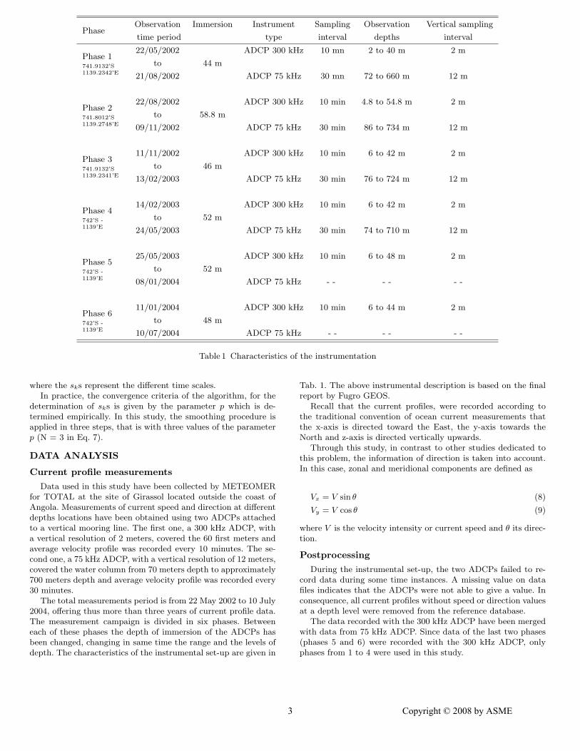
PhaseObservation Immersion Instrument Sampling Observation Vertical sampling

time period type interval depths interval

Phase 1741.9132’S

1139.2342’E

22/05/2002 ADCP 300 kHz 10 mn 2 to 40 m 2 m

to 44 m

21/08/2002 ADCP 75 kHz 30 mn 72 to 660 m 12 m

Phase 2741.8012’S

1139.2748’E

22/08/2002 ADCP 300 kHz 10 min 4.8 to 54.8 m 2 m

to 58.8 m

09/11/2002 ADCP 75 kHz 30 min 86 to 734 m 12 m

Phase 3741.9132’S

1139.2341’E

11/11/2002 ADCP 300 kHz 10 min 6 to 42 m 2 m

to 46 m

13/02/2003 ADCP 75 kHz 30 min 76 to 724 m 12 m

Phase 4742’S -

1139’E

14/02/2003 ADCP 300 kHz 10 min 6 to 42 m 2 m

to 52 m

24/05/2003 ADCP 75 kHz 30 min 74 to 710 m 12 m

Phase 5742’S -

1139’E

25/05/2003 ADCP 300 kHz 10 min 6 to 48 m 2 m

to 52 m

08/01/2004 ADCP 75 kHz - - - - - -

Phase 6742’S -

1139’E

11/01/2004 ADCP 300 kHz 10 min 6 to 44 m 2 m

to 48 m

10/07/2004 ADCP 75 kHz - - - - - -

Table 1 Characteristics of the instrumentation

where the sks represent the different time scales.In practice, the convergence criteria of the algorithm, for the

determination of sks is given by the parameter p which is de-termined empirically. In this study, the smoothing procedure isapplied in three steps, that is with three values of the parameterp (N = 3 in Eq. 7).

DATA ANALYSIS

Current profile measurements

Data used in this study have been collected by METEOMERfor TOTAL at the site of Girassol located outside the coast ofAngola. Measurements of current speed and direction at differentdepths locations have been obtained using two ADCPs attachedto a vertical mooring line. The first one, a 300 kHz ADCP, witha vertical resolution of 2 meters, covered the 60 first meters andaverage velocity profile was recorded every 10 minutes. The se-cond one, a 75 kHz ADCP, with a vertical resolution of 12 meters,covered the water column from 70 meters depth to approximately700 meters depth and average velocity profile was recorded every30 minutes.

The total measurements period is from 22 May 2002 to 10 July2004, offering thus more than three years of current profile data.The measurement campaign is divided in six phases. Betweeneach of these phases the depth of immersion of the ADCPs hasbeen changed, changing in same time the range and the levels ofdepth. The characteristics of the instrumental set-up are given in

Tab. 1. The above instrumental description is based on the finalreport by Fugro GEOS.

Recall that the current profiles, were recorded according tothe traditional convention of ocean current measurements thatthe x-axis is directed toward the East, the y-axis towards theNorth and z-axis is directed vertically upwards.

Through this study, in contrast to other studies dedicated tothis problem, the information of direction is taken into account.In this case, zonal and meridional components are defined as

Vx = V sin θ (8)

Vy = V cos θ (9)

where V is the velocity intensity or current speed and θ its direc-tion.

Postprocessing

During the instrumental set-up, the two ADCPs failed to re-cord data during some time instances. A missing value on datafiles indicates that the ADCPs were not able to give a value. Inconsequence, all current profiles without speed or direction valuesat a depth level were removed from the reference database.

The data recorded with the 300 kHz ADCP have been mergedwith data from 75 kHz ADCP. Since data of the last two phases(phases 5 and 6) were recorded with the 300 kHz ADCP, onlyphases from 1 to 4 were used in this study.

3 Copyright © 2008 by ASME

N % of total variance % of cumulative variances Residue (%)AD LL UL AD LL UL AD LL+UL

1 53.26 56.98 68.44 53.26 56.98 68.44 52.80 42.652 19.79 24.57 18.48 73.05 81.56 86.93 35.27 24.593 12.33 7.03 7.21 85.39 88.59 94.14 24.34 18.254 7.42 5.73 3.11 92.82 94.33 97.26 17.76 14.765 4.75 3.07 1.78 97.57 97.40 99.04 13.55 12.83

Table 2 EOF approximation. AD : All Data, LL : Lower Layer, UL : Upper Layer

Observing Tab. 1, we can see that each phase doesn’t corres-pond to the same depth of immersion of the instrumentation andas we have seen previously, the averaging period was 10 minutesfor the 300 kHz ADCP and 30 minutes for the 75 kHz ADCP.Hence, in order to have a common range in time and space foreach phase we need to interpolate data. Data from the the 300kHz ADCP were resampled with a time increment of 10 minutesand space increment of 2 meters form 6 to 40 meters (18 levels).Whereas those from the 75 kHz ADCP have been interpolatedfrom 88 to 652 meters with a constant step of 12 meters (48levels).

The maximum current speed in the reconstructed data file isfound to be close to 0.76 m/s, which occurred at depth of 22 mbelow mean sea-level (MSL) on 16 February 2003 at 17 :30 GMT.The maximum in the lower water column is close to 0.38 m/s at148 m below MSL.

Fig 1 shows different types of current profiles, correspondingto a current profile for which the average is greater than 0.20m/s. For each figure, the red star is the extremity of 6 m depthcurrent vector and the black dot points the extremities of theother current vectors. The left view is a 3D view of the profilewith a current vector each 2 meters in the upper layer and 12meters in lower layer. The middle view is the modulus (intensityor current speed) of each current vector. The right view is a topview of the first, where the origin of the current vector is indicatedby the black star.

0 0|V(z)| V(x,y;z)

This first visual analysis of the current profiles shows the com-plexity of current along the depth. However, we can observe thatcurrent speed generally decreases with depth and current direc-tion is highly variable near the surface.

EOF analysis on current data

The EOF method described above has been applied to themeasured current velocity data. Before applying the EOF tech-nique data was first transformed into two components : a North-South (N-S) component and an East-West (E-W) component.The results are shown in Tab. 2. One can observe how EOF me-thod can reduce the volume of data, since about 93% of the va-riance can be explained by the first four modes with a residue εequal to 17%.

The first three EOFs are plotted in Figs. 2, 3 and 4. The firstEOF is stronger in the upper layer than in the lower layer andit is very close to an unidirectional profile. Whereas, the secondand the third EOFs are sheared profiles with a rotating profilein the upper layer. The observations above confirm what we haveobserved graphically (see Fig. 1), that is the current flow in theupper layer is different from the flow of the lower layer. So, whenwe analyse separately the two layers, see Tab. 2, we observe thatthree EOFs are necessary in order to take into account morethan 94% of the total variance in the upper layer, whereas fourEOFs are needed in the lower layer. These results show that thedecomposition using each layer doesn’t simplify the complexityof the current profiles.

|V(z)| V(x,y;z)

−1 0 1−1

01

−700

−600

−500

−400

−300

−200

−100

dept

h (m

)

0 0.5 1−700

−600

−500

−400

−300

−200

−100

speed (m/s)

dept

h (m

)

−0.2 −0.1 0 0.1−1

−0.8

−0.6

−0.4

−0.2

0

0.2

0.4

Vx speed (m/s)

Vy s

peed

(m

/s)

Fig. 1 Current profile no 628

−0.500.5

−0.50

0.5

−700

−600

−500

−400

−300

−200

−100

0

dept

h (m

)

0 0.2 0.4−700

−600

−500

−400

−300

−200

−100

0

speed (m/s)

dept

h (m

)

0 0.05 0.1

−0.2

−0.1

0

0.1

0.2

0.3

0.4

Vx speed (m/s)

Vy s

peed

(m

/s)

Fig. 2 First EOF profile

4 Copyright © 2008 by ASME

−0.500.5

−0.50

0.5

−700

−600

−500

−400

−300

−200

−100

0

dept

h (m

)

0 0.1 0.2−700

−600

−500

−400

−300

−200

−100

0

speed (m/s)

dept

h (m

)

|V(z)|

−0.1 0 0.1

−0.4

−0.2

0

0.2

0.4

0.6

Vx speed (m/s)

Vy s

peed

(m/s

)

V(x,y;z)

Fig. 3 Second EOF profile

−0.50

0.5

−0.50

0.5

−700

−600

−500

−400

−300

−200

−100

0

dept

h (m

)

0 0.2 0.4−700

−600

−500

−400

−300

−200

−100

0

speed (m/s)

dept

h (m

)

|V(z)|

−0.2 0 0.2

−0.8

−0.6

−0.4

−0.2

0

0.2

0.4

0.6

0.8

Vx speed (m/s)

Vy s

peed

(m/s

)

V(x,y;z)

Fig. 4 Third EOF profile

Current time scales

As mentioned earlier, another part of the difficulty in the mo-delling of current profiles comes from the superposition of variousphysical processes of circulation, which occur at different timescales.

The few results hereafter show some characteristics of the timescales of the entire column water. They have been obtained withlevel 88 meters under the surface.

The observation of the covariance functions for zonal and meri-dional components, Fig 5 top, shows clearly different time scales.A very low process, with a period approximately equal to 90days, corresponding to the general circulation. A second with aperiodicity of approximately 3.5 days, represent the inertial cur-rents and a last one, Fig 5, bottom, with a period of 0.5 day(semi-duirnal tide). Inertial and tide periodicity can be verifiedby the theory. In case of the inertial currents the period is givenby formula 12/sin(latitude), which gives here 3.7 days. Observealso that the inertial component correlation vanishes with timelags, which is not the case with the tidal component as it is a

5

periodical phenomena.By plotting the spectral density, Fig 7, we can see in detail the

tidal components : diurnal sun and moon tides with respectiveperiods of 1 day-1 and 0.93 day-1 and semidiurnal sun and moontides with periods 2 day-1 and 1.93 day-1.

0 10 20 30 40 50 60 70 80 90 100−2

0

2

4

6x 10

−3 Current N−S & E−W components (depth 88 )

lag (day)

Cu

rre

nt co

va

ria

nce

(m

2/s

2) E−W

N−S

0 5 10 15 20 25 30−2

0

2

4

6x 10

−3

lag (day)

Cu

rre

nt co

va

ria

nce

(m

2/s

2)

Fig. 5 Covariance functions, N-S and E-W components

0 0.5 1 1.5 2 2.50

0.5

1

1.5

2

2.5

3

3.5

4Current N−S component (depth 88 )

frequency (day−1)

powe

r spe

ctral

dens

ity

Fig. 6 Spectral density, N-S component

0 0.5 1 1.5 2 2.50

0.5

1

1.5

2

2.5

3

3.5

4Current E−W component (88 m)

frequency (day−1)

powe

r spe

ctral

dens

ity

Fig. 7 Spectral density, E-W component

Copyright © 2008 by ASME

The processing of the current time series decomposition in thedifferent time scales is obtained using cubic smoothing splines asdescribed above. The smoothing parameter values used for thethree times scales are : p1 = 1.10−7, p2 = 2.10−4, p3 = 2.10−1.All the time series at the different time scales are given in Fig. 8.The first is the global circulation, the second inertial component,the third tidal component and the last the residue. The spectraldensity of the residue given for high frequency bands in Fig. 9,shows that it is close to white noise.

The use of the EOF method on each time scales have shownthat the number of EOF modes retained is approximately thesame when using the original data. So the complexity of the cur-rent profiles is not simplify when decomposing in time scales.

−0.5

0

0.5

(m/s

)

Current N−S decomposition (depth 88)

−0.5

0

0.5

(m/s

)

−0.5

0

0.5

(m/s

)

02/05 02/06 02/07 02/09 02/10 02/11 03/01 03/02 03/03 03/05 03/06−0.5

0

0.5

date (yy/mm)

(m/s

)

Fig. 8 Time series of different time scales

10 12 14 16 18 20 22 240

1

2

3

4

5

6

7x 10

−3 Current N−S component (depth 88)

frequency (day−1)

powe

r spe

ctral

dens

ity

Fig. 9 Spectral density of the residue for high frequency

6

PROBABILISTIC METHODS FOR CURRENT

PROFILES

The aim of this section is to evaluate the accuracy of the EOFmodelling. To do this two simplified approaches or criteria areconsidered. The first one is based on static calculus of the toptension (horizontal component) and the second is derived from amodal analysis used in a simplified VIV analysis. The compari-son criterion is carried out from extreme distributions calculatedfor all measured current profiles and compared with results fromEOF profiles.

More Precisely, we want to calculate the distribution functiondefined by

IP (G(V (t, z)) > g) (10)

where G, defined by the two above criteria, is determined fromeach measured current profiles in the original data set and eachcurrent profiles from EOF approximation based upon four EOFsmodes.

Practically, from each current profiles in the original data,[V (t, z)], The function G is calculated. Once the function G iscalculated, the inverse cumulative distribution function or thecumulative distribution function is empirically determined. Thesame procedure is applied to each current profiles from the re-constructed matrix [V̂ (t, z)] obtained using four EOFs.

This analysis requires the construction of a riser model. Thestudied case is a flexible riser tensioned at the top, whose themain characteristics are listed in Tab. 3.

Parameters

Model length 658 mOuter diameter 340 mmMass of riser 210 kg/m

Young’s Modulus 4.4 109 NBottom tension 0.3 106 N

Top tension 1.0656 106 N

Table 3 Main characteristics of the riser model considered

Vortex induced vibrations is a resonant response to fluctua-ting lift forces due to alternate vortex shedding in the flow pastthe riser. It is generally acknowledged that significant VIV occurwhen the reduced velocity Vr = Vc/Dfs, where Vc is the cur-rent velocity, D the riser outer diameter and fs the frequency ofone of the riser flexural eigenmodes, is in the range [4, 10] with amaximum response for Vr around 6.

Let V minr and V max

r be respectively the minimum and maxi-mum current values at all levels in the full database. The lowestpotentially excited eigenfrequency is fmin

s = 4D/V maxr , and the

highest is fmaxs = 10D/V min

r . Using the DeeplinesTM riser model,we compute the eigenfrequencies fi that fall within the interval[fmin

s , fmaxs ].

For a given current profile, referring to an appropriate VIVamplitude versus Vr curve, we compute the amplitude obtainedat each level and for each eigenmode ψi of the corresponding ei-genfrequency fi. This taken as a measure of the contribution ofeach level to the excitation of eigenmode ψi. The contributionsfrom all current levels to each eigenmode ψi are summed up. The

Copyright © 2008 by ASME

riser is supposed to respond on the eigenmode for which the sumof the contributions from all current levels, regardless of direc-tion, is maximum. The VIV criteria is an estimate of the fatiguerate based on previously computed excitation level, multiplied bya factor related to the modal deflection maximum curvature. Fur-ther developments are to be achieved later to ensure this approachis consistent with widely accepted methods such as DeepVIVTM

or Shear7TM.The results are shown in Figs. 10 and 11. In these figures the

estimated cumulative distribution function (CDF), based uponmeasured current profiles and four EOFs are plotted on a Gumbelplot. Since we are interested in extreme values, only values withhigh probability are considered.

Concerning the first criteria, one can observe (see Fig. 10)that current profiles based upon 4 EOFs, for a probability of 0.9,overestimate the top tension in order of 17%. Whereas, for thesecond criteria (see Fig. 11) EOF approximation underestimatesthe VIV criteria in order of 5%.

When observing the above results it is surprising that withthe first criteria four EOFs overestimate the top tension whereasusing the second criteria four EOFs cause underestimation of theamplitude of the excited modes. At this stage, there no reasonthat can explain this fact. So in order to ensure conservatismfurther developments may be achieved.

In case of the VIV criteria a study of Meling et al (2002) hasshown that by increasing the number of EOF modes one canpasses from a non-conservative state to a conservative state.

1000 1200 1400 1600 1800 2000 2200 2400 2600

0.90

0.96

0.99

0.999

0.9999

Top tension (N)

P[F(

v(t,z)

) ≤ f]

Gumbel Probability Plot

Measured dataEOF approximation

Fig. 10 Distribution of the top tension (Gumbel plot)

0.16 0.18 0.2 0.22 0.24 0.26 0.28

0.90

0.96

0.99

0.999

0.9999

Amplitude of VIV (m)

P[F(

v(t,z)

) ≤ f]

Gumbel Probability Plot

Measured dataEOF approximation

Fig. 11 Distribution of the VIV amplitude mode (Gumbelplot)

ACKNOWLEDGEMENTS

Total is acknowledged for its contribution to the funding ofthis work and for the permission to publish the results of thepresent study.

CONCLUSION

This paper deals with statistical modelling of current profilesfor risers design. This work is based on current profiles measure-ments from the site of Girassol in West Africa. Various aspects toderive reliable statistical modelling of current profiles have beenconsidered. First, using the whole data (speed and direction), theEOF approach has been used to reduce current profiles. It hasbeen shown that only four EOFs, representing 93% of the totalvariance, are necessary to represent the original current profiles.Considering separately the upper and the lower layer, the firstfour modes contributed more than 97% of the total variance inthe upper layer of the water column. In the lower layer, theyrepresent approximately 94% of the total variance. Secondly, theidentification of time series of different time scales by mean ofcubic splines has been presented. Even though this method isdifficult in parametrization, it is of great interest in data withmissing values. The use of EOF method with each time scale donot improve the results, that is the number of EOFs consideredis approximately the same when we use the original data.

Different probabilistic approaches for riser design can becombined with EOF analysis. In this study, the EOF modellinghas been validated through extreme distributions using twosimplified criteria. The first is based on static calculus and thesecond is derived from a VIV analysis. We found with the lastcriteria that the error made is in order of 5% whereas, with thefirst criteria the error is about 17%.

Recall that this work is a part of a global project which consistsin using results from EOF analysis of current profiles in reliabi-lity approaches such as, FORM (First Order Reliability Method),SORM (Second Order Reliability Method) and Monte Carlo si-mulations. These last methods involve first the determination ofthe climatology of current profile (marginales or joint distribu-tions of coefficients) which is difficult to determine when the num-ber of coefficients is higher. So the use of the EOF method allowus, instead of working in a dimension space equal to the numberof depth level (that is 66), to work on a dimension space equal tothe number of considered EOFs (that is 4), showing in the sametime the efficiency gained by using EOF method.

7 Copyright © 2008 by ASME

REFERENCES

[1] Jeans, G., Grant, C., and Feld, G., 2002, ”Improved CurrentProfile Criteria for Deepwater Riser Design”, Journal of Off-shore Mechanics and Arctic Engineering, vol 125, pp. 221-224.

[2] Forristall, G. Z., and Cooper, C. K., 1997, ”Design CurrentProfiles Using Empirical Orthogonal Function (EOF) and In-verse FORM Methods”, Proceedings of the 29th Annual Off-shore Technology Conference, OTC 8267, Houston, Texas.

[3] Meling, T. S., Eik, K. J., and Nygaard, E., 2002, ”An As-sessment of EOF Current Scatter Diagrams with Respect toRiser VIV Fatigue Damage”, Proceedings of the 21st Interna-tional Conference of Offshore Mechanics and Arctic Enginee-ring, OMAE2002-28062, Oslo, Norway.

[4] Neves, S. N., and Soares, C. G., 2004, ”Modelling Tidal Cur-rent Profiles by Means of Empirical Orthogonal Functions”,Proceedings of OMAE Speciality Conference on Integrity ofFloating Production, Storage & Offloading (FPSO) Systems,OMAE-FPSO’O4-0044, Houston, Texas.

[5] Lambrakos, K. F., Sidarta, D. E., Thompson, H. M., Steen,A., and Burke, R.W., 2005, ”Method for Reducing a LargeNumber of Current Profiles to a Small Subset for Riser VIVAnalysis”, Proceedings of the 21st International Conferenceof Offshore Mechanics and Arctic Engineering, OMAE2005-67279, Halkidiki, Greece.

[6] Huang, N. E., Shen, Z., Long, S. R., Wu, M. C., Shih, H. H.,Zheng, Q., Yen, N.-C., Tung, C. C., and Liu, H. H., 1998, ”TheEmpirical Mode Decomposition and the Hilbert Spectrum forNonlinear and Non-Stationary Time Series Analysis”, Proc.R. Soc. Lond. A, 454, pp. 903-995.

[7] Wahba, G., 1990, ”Splines Models for Observational Data”,SIAM.

[8] Green, P., and Silverman, B., 1994, ”Nonparametric Regres-sion and Generalized Linear Models : a Roughness PenaltyApproach”, Chapman and Hall.

8 Copyright © 2008 by ASME