Statistical Modeling of Spot Instance Prices inPublic Cloud Environments

Bahman Javadi∗, Ruppa K. Thulasiram†, and Rajkumar Buyya∗∗ Cloud Computing and Distributed Systems (CLOUDS) Laboratory

Dept. of Computer Science and Software Eng., The University of Melbourne, Australia

Email: bahmanj, raj@csse.unimelb.edu.au† Computational Financial Derivatives (CFD) Laboratory

Department of Computer Science, University of Manitoba, Winnipeg, Canada

Email: tulsi@cs.umanitoba.ca

Abstract—The surge in demand for utilizing public Cloudresources has introduced many trade-offs between price, per-formance and recently reliability. Amazon’s Spot Instances (SIs)create a competitive bidding option for the public Cloud usersat lower prices without providing reliability on services. Itis generally believed that SIs reduce monetary cost to theCloud users, however it appears from the literature that theircharacteristics have not been explored and reported. We believethat characterization of SIs is fundamental in the design ofstochastic scheduling algorithms and fault tolerant mechanismsin public Cloud environments for spot market. In this paper, wehave done a comprehensive analysis of SIs based on one yearprice history in four data centers of Amazon’s EC2. For thispurpose, we have analyzed all different types of SIs in terms ofspot price and the inter-price time (time between price changes)and determined the time dynamics for spot price in hour-in-dayand day-of-week. Moreover, we have proposed a statistical modelthat fits well these two data series. The results reveal that we areable to model spot price dynamics as well as the inter-price timeof each SI by the mixture of Gaussians distribution with threeor four components. The proposed model is validated throughextensive simulations, which demonstrate that our model exhibitsa good degree of accuracy under realistic working conditions.

Keywords-Cloud Computing; Spot Price; Statistical Model;

I. INTRODUCTION

Due to the surge in demand for using utility computing

systems like public Cloud resources, many trade-offs between

price and performance have emerged. One particular type

of Cloud service, which is known as Infrastructure-as-as-

Service (IaaS) provides raw computing with different capacity

and storage in the form of Virtual Machines (VMs) with

various prices on a pay-as-you-go basis. For instance, Amazon

provides on-demand and reserved VM instances, which are

associated with a fixed set price [13]. However, Amazon can

increase or decrease these prices based on their own local

policy. There are 64 different types of instances with various

capacities and prices under two operating systems (i.e. 32

for Linux and 32 for Windows) which are made available by

Amazon in four data centers as illustrated in Table I (sorted

by their prices). In this Table, the prices are given for Linux

operating system and the instances labeled with ’m1’, ’m2’,

and ’c1’ are standard, high-memory, and high-CPU instances,

respectively.

In December 2009, Amazon released a new type of in-

stances called Spot Instance (SI) to sell the idle time of

Amazon’s EC2 data centers [3]. The price of an SI, spot price,

depends on the type of instance as well as VM demand within

each data center. In fact, spot instances are an alternative to

other two classes of instances which offer a low price but less

reliable and competitive bidding option for the public Cloud

users. Therefore, another aspect, reliability, has been added to

the existing trade-offs to make utility computing systems more

challenging than ever.In order to utilize SIs, the Cloud users provide a bid which is

the maximum price to be paid for an hour of usage. Whenever

the current price of an SI is equal or less than the user bid,

the instance is made available to the user. If the price of an SI

becomes higher than the user’s bid, out-of-bid event (failure),

the VM(s) will be terminated by Amazon automatically and

user does not pay for any partial hour. However, if the user

terminates the running VM(s), she has to pay for the full hour.

Amazon charges users per hour by the market price of the SI

at the time of VM creation.There are a limited number of works on how to utilize SIs

to decrease the monetary cost of utility computing for Cloud

users [12], [14]. However, a thorough statistical analysis and

modeling of SIs have not been appeared in the literature, the

focus of our research in this study. In this paper, we provide

a comprehensive analysis of all SIs in terms of spot price

and the inter-price time (time between price changes) in four

Amazon’s data centers (i.e. us-west, us-east, eu-west, and ap-

southeast). Moreover, we propose a statistical model to capture

the volatile spot prices in Amazon’s data centers. The main

contributions of this paper are as follows:

• We provide statistical analysis for all SIs in Amazon’s

EC2 data centers. We also determine the time correlation

in spot price in terms of hour-in-day and day-of-week.

• We model spot price and the inter-price time of each

SI with the mixture of Gaussians distribution. A model

calibration algorithm is also proposed to deal with an

observed price trend in the real price history.

• We validate and verify the accuracy of our proposed

model through simulation under realistic working con-

ditions.

2011 Fourth IEEE International Conference on Utility and Cloud Computing

978-0-7695-4592-9/11 $26.00 © 2011 IEEE

DOI 10.1109/UCC.2011.37

219

TABLE IPRICES OF ON-DEMAND INSTANCES IN DIFFERENT DATA CENTERS OF AMAZON (PRICES GIVEN IN CENTS).

Instances us-west us-east eu-west ap-southeast EC2 Compute Unit Memory (GB) Storage (GB)m1.small 9.5 8.5 9.5 9.5 1 1.7 160c1.medium 19 17 19 19 5 1.7 350m1.large 38 34 38 38 4 7.5 850m2.xlarge 57 50 57 57 6.5 17.1 420m1.xlarge 76 68 76 76 8 15 1690c1.xlarge 76 68 76 76 20 7 1690m2.2xlarge 114 100 14 114 13 34.2 850m2.4xlarge 228 200 228 228 26 68.4 1690

We believe that results of this research would significantly

helpful in the design of stochastic scheduling algorithms and

fault tolerant mechanisms (e.g. checkpointing and replication

algorithms) for spot market in public Cloud environments.

Moreover, this model can be used by other IaaS Cloud

providers that look forward to offer such a service in the near

future.

The paper is structured as follows. In Section II, we describe

the processes that we model in this paper. We discuss related

work in Section III. We examine the pattern of spot price in

Section IV. In Section V, we present the global statistics for

all SIs. We then illustrate distribution fitting for spot price and

the inter-price time in Section VI. In Section VII, we propose

an algorithm for model calibration. We discuss the validation

of the proposed models through simulation in Section VIII.

In Section IX, we summarize our contributions and describe

future directions.

II. MODELING APPROACH

In this section, we describe two variables that we are going

to analyze and model. In Amazon’s data centers, SIs have two

variables (i.e. spot price and inter-price time) specified by the

Cloud provider and one variable (user’s bid) determined by

users. In this study, we focus on the analysis and modeling

of spot price and the inter-price time as two highly volatile

system variables. These variables are illustrated in Figure 1

where Pi is the price of an SI at time ti. So, the inter-price

time is defined as Ti = ti+1− ti. Therefore, the time series of

spot price (Pi) and the inter-price time (Ti) are analyzed and

modeled in the following sections.

Fig. 1. Spot price and the inter-price time of Spot instances.

The traces that we use in this study are one year price

history of all Amazon SIs from the first of February 2010

to mid-February 2011. We use the first 10-month (Feb-2010

to Nov-2010) in the modeling process. These 10-month traces

along with the last 2-month are used for the model validation

purpose. The spot price history is freely provided by Amazon

per SI for each data center and also available through other

third-parties such as [1]. We do not use data prior to February

2010 due to an algorithm issue reported in [2] for prices.

Moreover, we only use the SIs with Linux operating systems

from all data centers. Due to space limitation as well as

similarity of the results, we present our findings for only one

data center (i.e. eu-west). Interested readers can refer to the

extended version of this paper [9] for more discussions about

other data centers.

III. RELATED WORK

To the best of our knowledge, this is the first work to ana-

lyze and model spot instances in public Cloud environments.

However, there are some papers which investigated the usage

of SIs to decrease the monetary cost of utility computing.

Yi et al. [14] introduced some checkpointing mechanisms

for reducing cost of SIs. They used the real price history of

EC2 spot instances and showed how the adaptive checkpoint-

ing schemes could decrease the monetary cost and improve

the job completion times. In [4], a decision model for the

optimization of performance, cost and reliability under SLA

constraints while using SIs is proposed. They used the real

price history and workload models to demonstrate how their

proposed model can be used to bid optimally on SIs to reach

different objective with desired levels of confidences.

Chohan et al. in [6] proposed a method to utilize the SIs

to speed up the MapReduce tasks. They provided a Markov

chain to predict the expected lifetime of an SI. They concluded

that having a fault tolerant mechanism is essential to run

MapReduce jobs on SIs. Also, in [12], authors proposed a

hybrid Cloud architecture to lease the SIs to manage peak

loads of a local cluster. They proposed some provisioning

policies and investigated the utilization of SIs compared to

on-demand instances in terms of monetary cost saving and

number of deadline violations.

Although the current literature shows that SIs are good

alternative for on-demand or reserve instances in terms of

monetary cost, the characteristics of SIs are not clear to users

and researchers in the community. Hence, for this research

we propose to devise a statistical model for SIs for better

understanding of the price mechanisms in Amazon’s data

centers.

220

(a) Hour-in-day (b) Day-of-week

Fig. 2. Patterns of spot price in eu-west data center.

IV. PATTERNS OF SPOT PRICE

In this section, we examine hour-in-day and day-of-week

time dynamics for the price of different SIs in eu-west data

center. We use the same approach as [11] to show how the

price of one SI changes each hour in the day or each day of

the week. As we have the price history in GMT time zone,

we adjusted the local time for the time zone. This adjustment

could reveal the dependency of spot price on the local time

of a data center. In Figure 2(a), we create eight 3-hour time

slots per day, and determine the average price of each SI in

each time slot over all days. Then, we normalized this average

by the maximum average price over all days. Note that the

frequency of 3-hour sampling could be increased to 1-hour

sampling with 24 time slots in a day. However, it would only

increase the sample size without shedding much light on the

price dynamics, since spot price in Amazon’s data centers are

changing at the earliest every 2-3 hours (see Section V).

In Figure 2(b), we applied the same procedure to obtain the

average price over seven 24-hours time slots within a week.

In Figure 2(a), we can see that the y-axis is in the range of

[0.98 1.0] where there is an increasing trend over the first-half

of each day ([0 12]) and decreasing trend in spot price during

the second-half of each day for all SIs in this data center.

The y-axis in Figure 2(b) has wider range of [0.91 1.0]

for eu-west data center1. As it is observable from this plot,

we can not find any specific pattern for spot price, except

the decreasing in prices on weekends. However, for other

Amazon’s data centers, we see more clear patterns in day

of the week where on Tuesday we have the maximum price

for almost all SIs in those data centers. Moreover, the lowest

price are on Saturday, but on Sunday we again observe the

increasing in price for all SIs. These facts are more pronounced

in us-east and ap-southeast data centers [9].

1For other data centers, this range is narrower ([0.95 1.0]).

V. GLOBAL STATISTICS AND ANALYSIS

In the following, we analyze the price history of different

SIs in eu-west data center. We inspect the basic statistics

of the traces in terms of spot price in Table II; and in

terms of the inter-price time in Table III. The statistics in

the tables are mean, trimmed mean (the mean value after

discarding 10% of extreme values), median, standard deviation

(Std), coefficient of variance (CV), interquartile range (IQR),

maximum, minimum, skewness (the third moment), kurtosis

(the forth moment) and number of samples.

These tables show three types of descriptive statistics.

Statistics of the first type (mean, median, trimmed mean)

reveal the central tendency of the distributions. Statistics of

the second type (CV, IQR, minimum, maximum) reflect the

spread of the distributions. Statistics of the third type (kurtosis,

skewness) represent the shape of the distributions.

First of all, we find that on average the price of SIs can

be as low as 44% of on-demand instances (this percentage

is 38%, for us-east data center which is the cheapest data

center). This expresses that there are some opportunities in

reducing monetary cost of utility computing at the cost of

unreliability. Moreover, the maximum price of some SIs (like

m1.large) is bigger than the price of corresponding on-demand

instance (specially in us-east data center). Thus, even if the

users’ bid is as high as the on-demand prices, we may still

have a probability of out-of-bid events.

The results in these tables reveal that the ratios between

the mean and the median for spot price and the inter-price

time of SIs are close to 1 for each trace. This indicates

that Gaussian distribution might be a good option for the

model. However, the skewness and kurtosis values show that

the underlying distributions are right-skewed and short-tailed.

Therefore, Gaussian distribution may not be a representative

model to use and a better distribution is in order.

221

TABLE IISTATISTICS FOR SPOT PRICE IN EU-WEST DATA CENTER (VALUES GIVEN IN CENTS).

Instances Mean TrMean Median Std CV IQR Max Min Skewness Kurtosis No.m1.small 4.00 4.00 4.00 0.19 0.05 0.20 9.50 3.80 9.44 242.97 3702c1.medium 8.00 8.00 8.00 0.27 0.03 0.40 10.10 7.60 0.28 3.91 3812m1.large 16.04 16.02 16.10 0.85 0.05 1.00 50.00 15.20 21.55 792.41 3875m2.xlarge 24.04 24.03 24.10 1.03 0.04 1.40 57.10 22.80 12.91 387.69 3763m1.xlarge 32.05 32.01 32.10 1.60 0.05 2.00 76.00 30.40 15.34 415.47 3917c1.xlarge 32.04 32.03 32.10 1.07 0.03 2.00 45.00 30.40 0.54 8.27 3658m2.2xlarge 56.04 56.04 56.20 1.83 0.03 3.42 76.00 53.20 0.25 4.99 4001m2.4xlarge 112.08 112.08 112.50 3.62 0.03 6.80 150.00 106.40 0.21 4.55 3912

TABLE IIISTATISTICS FOR THE INTER-PRICE TIME IN EU-WEST DATA CENTER (VALUES GIVEN IN HOURS).

Instances Mean TrMean Median Std CV IQR Max Min Skewness Kurtosis No.m1.small 1.96 1.61 1.35 2.66 1.35 0.30 109.08 0.02 19.94 727.54 3701c1.medium 1.91 1.59 1.34 1.86 0.97 0.32 22.81 0.02 4.53 30.63 3811m1.large 1.88 1.57 1.33 1.79 0.95 0.31 30.94 0.02 5.02 42.02 3874m2.xlarge 1.79 1.53 1.34 1.56 0.87 0.30 22.83 0.02 4.93 38.54 3762m1.xlarge 1.86 1.58 1.34 1.78 0.96 0.31 38.20 0.02 7.34 101.43 3916c1.xlarge 1.99 1.56 1.34 7.22 3.63 0.30 378.19 0.02 44.38 2169.40 3657m2.2xlarge 1.82 1.55 1.33 1.60 0.88 0.31 29.02 0.02 5.11 45.75 4000m2.4xlarge 1.86 1.58 1.34 1.71 0.92 0.31 26.51 0.02 5.20 44.28 3911

Additionally, we can observe that the inter-price time is

more variable than spot price due to higher values of coef-

ficient of variance. Also, analysis of the trimmed mean con-

firmed that inter-price time has greater variability. Therefore,

we may need distributions with higher degrees of freedom, to

model the inter-price time for these traces. It is worth noting

that the minimum inter-price time is almost one hour in all

data centers except eu-west which is about a few minutes and

can be seen in Table III). Moreover, in eu-west data center,

the set price of SIs are stable on average for less than two

hours, where for other data centers this duration is about 2-

3 hours [9]. This is the justification of 3-hour time slots to

examine patterns of spot price in Figure 2(a).

VI. DISTRIBUTION FITTING

After global statistical analysis, we first inspect the Proba-

bility Density Function (PDF) of spot price and the inter-price

time. Then, we conduct parameter fitting for the Mixture of

Gaussians (MoG) distribution by the expectation maximization

(EM) algorithm to model both time series. We considered

other distributions, such as Weibull, Normal, Log-normal

and Gamma distributions as well. However, the mixture of

Gaussians distribution shows the better fit with respect to

others [9].

A. Probability Densities

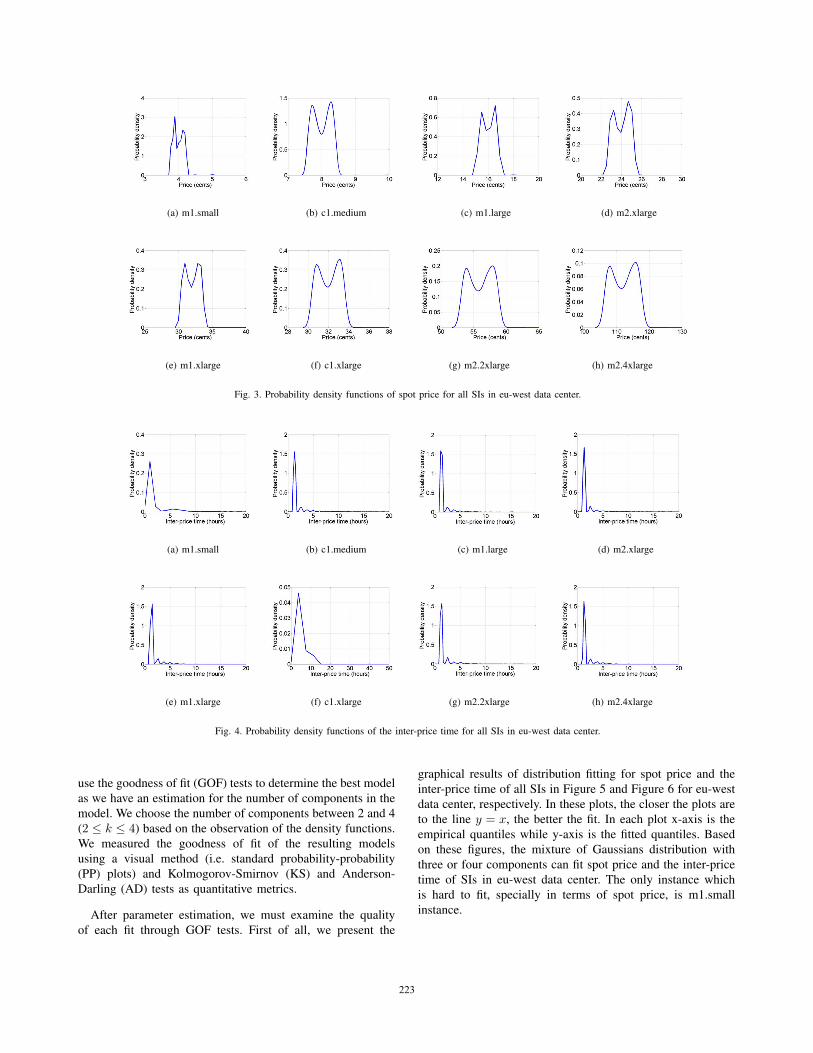
The PDFs of spot price of each SI in eu-west data center

are depicted in Figure 3. We can easily observe bi-modality in

the probability density functions. Moreover, the price distri-

bution of all SIs, except m1.small, are almost symmetric. The

exception for m1.small is possibly because of diverse usage

patterns of this instance as the cheapest resource in each data

center.

The PDFs of the inter-price time for each SI in eu-west

are represented in Figure 4. Obviously, there is a single

dominant mode (peak) in the density functions when compared

to (nearly) equal peaks in the PDFs of spot price. Most of SIs

have the peak around two hours, which confirm the results

of the previous section (see Mean column in Table III). The

reason for the very sharp peak in these density functions

is investigated in Section VII. Observation from the plotted

density functions of both time series, our decision to propose

a mixture of Gaussians distribution as a good candidate for

approximating such density shapes is further strengthened.

B. Parameter Estimation and Goodness of Fit Tests

In this section, we conduct parameter fitting for the mixture

of Gaussians distribution with k components, which is defined

as follows:

cdf(x; k, �p, �μ, �σ2) =

k∑i=1

pi2

(1 + erf(

x− μi

σi

√2)

)(1)

where �μ, �σ2, and �p are the vector of mean, variance and

probability of components with k items. Also, erf() is the

error function, which is defined as follows:

erf(x) =2√π

∫ x

0

e−t2dt (2)

To maximize the data likelihood in terms of parameters �μand �σ2 where k is given a priori, we adopt the expectation

maximization (EM) algorithm, which is a general maximum

likelihood estimation. Parameter fitting was done using Model

Based Clustering (MBC), which is introduced by Fraley and

Raftery [7]. MBC is a methodological framework that can be

used for data clustering as well as (multi)variate density esti-

mation. One assumption is that data has several components

each of which is generated by a probability distribution. Model

Based Clustering uses Bayesian model selection to choose the

best model in terms of number of components. In contrast, we

222

(a) m1.small (b) c1.medium (c) m1.large (d) m2.xlarge

(e) m1.xlarge (f) c1.xlarge (g) m2.2xlarge (h) m2.4xlarge

Fig. 3. Probability density functions of spot price for all SIs in eu-west data center.

(a) m1.small (b) c1.medium (c) m1.large (d) m2.xlarge

(e) m1.xlarge (f) c1.xlarge (g) m2.2xlarge (h) m2.4xlarge

Fig. 4. Probability density functions of the inter-price time for all SIs in eu-west data center.

use the goodness of fit (GOF) tests to determine the best model

as we have an estimation for the number of components in the

model. We choose the number of components between 2 and 4

(2 ≤ k ≤ 4) based on the observation of the density functions.

We measured the goodness of fit of the resulting models

using a visual method (i.e. standard probability-probability

(PP) plots) and Kolmogorov-Smirnov (KS) and Anderson-

Darling (AD) tests as quantitative metrics.

After parameter estimation, we must examine the quality

of each fit through GOF tests. First of all, we present the

graphical results of distribution fitting for spot price and the

inter-price time of all SIs in Figure 5 and Figure 6 for eu-west

data center, respectively. In these plots, the closer the plots are

to the line y = x, the better the fit. In each plot x-axis is the

empirical quantiles while y-axis is the fitted quantiles. Based

on these figures, the mixture of Gaussians distribution with

three or four components can fit spot price and the inter-price

time of SIs in eu-west data center. The only instance which

is hard to fit, specially in terms of spot price, is m1.small

instance.

223

(a) m1.small (b) c1.medium

(c) m1.large (d) m2.xlarge

(e) m1.xlarge (f) c1.xlarge

(g) m2.2xlarge (h) m2.4xlarge

Fig. 5. PP-plots of spot price in eu-west for mixture of Gaussians (k = 2, k = 3, k = 4). X-axis: empirical quantiles, and Y-axis: fitted quantiles.

To be more quantitative, we also report the p-values of

two GOF tests (i.e. KS and AD tests). We randomly select

a subsample of 50 of each trace and compute the p-values

iteratively for 1000 times and finally obtain the average p-

value. This method is similar to the one used by the authors

in [10].

The results of GOF tests are listed in Table IV and Table V

for spot price and the inter-price time in eu-west, respectively.

Moreover, in each row the best fits are highlighted. In some

cases, we have two winners as there is one best fit per

each GOF test. These quantitative results strongly confirm the

graphical results of the PP-plots. The p-values in the first row

of Table IV express that spot price of m1.small instance is

hard to fit, even with four components. This is the case for

other data centers as well, specially for us-east data center [9].

As the number of parameters in the MoG distribution is

3k + 1 (see Equation 1), so we have a trade-off between

accuracy and complexity of the model. With fewer compo-

nents, the analysis becomes simpler that gives reasonably

good fit to spot price and inter-price time with a compromise

of accuracy to some extent. This would significanly help

in understanding the data series on the first step. With this

understanding a model to better fit the data series with many

TABLE IVP-VALUES RESULTING FROM KS AND AD TESTS FOR SPOT PRICE.

Instances MoG (k = 2) MoG (k = 3) MoG (k = 4)m1.small 0.016 0.791 0.017 0.789 0.053 0.803c1.medium 0.211 0.779 0.217 0.791 0.224 0.790m1.large 0.113 0.678 0.319 0.752 0.354 0.754m2.xlarge 0.139 0.616 0.356 0.721 0.415 0.734m1.xlarge 0.134 0.570 0.369 0.708 0.431 0.706c1.xlarge 0.394 0.681 0.444 0.705 0.421 0.707m2.2xlarge 0.420 0.648 0.469 0.682 0.450 0.672m2.4xlarge 0.429 0.617 0.463 0.637 0.476 0.653

components can be designed. Hence, for the sake of simplicity

and homogeneity, in the rest of this paper we choose the model

with three components (k = 3) for both spot price and the

inter-price time for further analysis. The set of parameters for

MoG distributions for spot price and the inter-price time for

2 ≤ k ≤ 4 in all data centers are reported in [9].

VII. MODEL CALIBRATION

In this section, we look into the time evolution of spot

price and the inter-price time, which potentially can lead us to

obtain a more accurate model. For this purpose, we examine

the scatter plot of spot price and the inter-price time during

224

(a) m1.small (b) c1.medium

(c) m1.large (d) m2.xlarge

(e) m1.xlarge (f) c1.xlarge

(g) m2.2xlarge (h) m2.4xlarge

Fig. 6. PP-plots of the inter-price time in eu-west for mixture of Gaussians (k = 2, k = 3, k = 4). X-axis: empirical quantiles, and Y-axis: fitted quantiles.

Algorithm 1: Model Calibration Algorithm

Input: Traceinst, k

Output: CalDate,−−−−−→RCmps

1 Ts ← Traceinst.start.time;2 Te ← Traceinst.end.time;3 n← Sizeof(Traceinst);

4−−−→index← (c1, c2, . . . , cn) ci ∈ {1, . . . , k};

5−−→date← (d1, d2, . . . , dn) di ∈ {Ts . . . Te};

6 qa,b ← probability of component a in month b;

7−→Q ← {qa,b|a ∈ {1, . . . , k}, b ∈ {Ts . . . Te}};

8−→Qm ← {qf,e|qf,e < q0, qf,e ∈ −→Q};

9−−−→Cmps← {g|qg,h ∈ −→Qm};

10−−−−−→RCmps← {1, . . . , k} − −−−→Cmps ;

11 m← min{h|qg,h ∈ −→Qm};12 //Traceinst(m) is the trace for month m;13 Tms ← Traceinst(m).start.time;14 Tme ← Traceinst(m).end.time;15 z ← Sizeof(Traceinst(m));

16−−−−→Sindex← (c′1, c

′2, . . . , c

′z) c′i ∈ {1, . . . , k};

17−−−→Sdate← (d′1, d

′2, . . . , d

′z) d′i ∈ {Tms . . . Tme};

18 t← max{rl|−−−−→Sindex(rl) == g, l ∈ {1, . . . , z}};19 CalDate← −−−→Sdate(t);

TABLE VP-VALUES RESULTING FROM KS AND AD TESTS FOR THE INTER-PRICE.

Instances MoG (k = 2) MoG (k = 3) MoG (k = 4)m1.small 0.347 0.476 0.415 0.592 0.489 0.627c1.medium 0.382 0.546 0.390 0.566 0.380 0.566m1.large 0.390 0.552 0.387 0.573 0.400 0.574m2.xlarge 0.389 0.556 0.393 0.566 0.405 0.585m1.xlarge 0.369 0.526 0.391 0.564 0.406 0.581c1.xlarge 0.221 0.319 0.399 0.561 0.467 0.602m2.2xlarge 0.376 0.532 0.426 0.570 0.463 0.610m2.4xlarge 0.368 0.529 0.383 0.569 0.395 0.573

February 2010 till November 2010. Due to space limitation,

we just present the plots for m2.4xlarge instance. The results

are consistent for other instance types within the data center.

Figure 7(a) depicts the scatter plot of spot price for

m2.4xlarge in eu-west data center for the duration of the price

history. As it can be seen in this figure, there is no clear

correlation in spot price where they are evenly distributed in

a specific range (this range depends on the type of instances).

However, congestion of spot price is increased after mid-July

and this is the case for all SIs in eu-west data center. To

confirm this observation, we examine the scatter plot of the

inter-price time for this SI in Figure 7(b). We observe that

225

(a) Scatter plot of spot price for m2.4xlarge.

(b) Scatter plot along with the components’ distribution ofthe inter-price time for m2.4xlarge.

Fig. 7. Scatter plot of spot price and the inter-price time for m2.4xlarge.

inter-price time become suddenly shorter after mid-July. That

means, the frequency of changing price is increased while

spot price remains bounded within a small price range. The

inspection of other SIs within the data center reveals the same

result. This is also the reason of very sharp peak in density

functions of the inter-price time in Figure 4.

This trend is possibly due to some fine tunings made by

Amazon in their pricing algorithm. It is worth noting that

the same issue has been observed in other Amazon’s EC2

data centers in different dates. In us-east it happened in

August 2010, and in us-west and ap-southeast in January 2011

(Figures are plotted in [9]).

Focusing on the scatter plot of the inter-price time (MoG

model for k = 3) presented in Figure 7(b), we can see

that after mid-July only one component (i.e. component 3)

remains and other components collapsed to a small band.

As this observation is consistent over all SIs, we propose a

model calibration algorithm (Algorithm 1) to find the date

of collapsing (which is called calibration date) as well as

remaining component(s).

TABLE VITHE RESULTS OF MODEL CALIBRATION IN EU-WEST (k = 3).

Instances Calibration Dates Remaining Componentsm1.small 24-July 3c1.medium 15-July 1m1.large 15-July 3m2.xlarge 13-July 1m1.xlarge 23-July 1c1.xlarge 23-July 1m2.2xlarge 23-July 1,2m2.4xlarge 15-July 3

The algorithm needs the trace of the inter-price time of an

SI (Traceinst) and the number of components (k). The result

of mixture of Gaussians model with k components is−−−→index.

Also,−−→date is a vector, each element of which correspond

to each item of−−−→index. At first, the algorithm computes the

probability of each component in each month in the whole

trace and after that finds a list (−→Qm) where the probability

of one or more components is less than q0 (line 4-8). q0is a threshold value and we define it as low as 0.01 (i.e.

q0 = 0.01). The components that are not in this list are

remaining components (−−−−−→RCmps in line 10). The first month

in the list of−→Qm is the calibration month, called m (line 11).

Finally, the last occurrence of the component(s) in month mwould be the calibration date (CalDate), which is obtained

in line 13-19.

The results of applying this algorithm for all SIs in eu-west

data center are presented in Table VI where all calibration

dates are in July. Moreover, for all SIs, except m2.2xlarge,

only one out of three components remains after the calibration

date.

The last step of the model calibration is probability adjust-

ment where the probability of remaining component(s) must be

scaled up to one. This adjustment can be done by the following

formula:

pj =pj∑∀i

pii, j ∈ −−−−−→RCmps (3)

In other words, in the calibrated model for each SI, we just

change the probability of remaining component(s) after the

calibration date. In the following section, we investigate the

accuracy of the calibrated model with respect to the real price

history as well as the non-calibrated model.

VIII. MODEL VALIDATION

In order to validate the proposed model, we implemented

a discrete event simulator using CloudSim [5]. The simulator

uses the model or the price history traces to run the input

workload. We consider the case where the user requests for

one VM from one type of SI and runs whole jobs on that VM.

The total monetary cost of running the workload on an SI is

the parameter to be considered.

A. Simulation Setup

The workload that we use in our experiments is the work-

load traces from LCG Grid which is taken from the Grid

226

(a) m1.small (b) c1.medium (c) m1.large (d) m2.xlarge

(e) m1.xlarge (f) c1.xlarge (g) m2.2xlarge (h) m2.4xlarge

Fig. 8. Model validation for all SIs in eu-west for the modeling traces (Feb-2010 to Nov-2010).

Workloads Archive [8]. We use the first 1000 jobs of this

trace as the input workload for the experiments which is long

enough to reflect the behavior of spot price for different SIs.

We assume that one EC2 compute unit is equivalent of a

CPU core with capacity of 1000 MIPS2. As such, the selected

workload needs about two weeks (≈ 400 hours) to complete

on a single m1.small instance. For other instance types we

consider the linear speedup with the computing capacity in

terms of EC2 compute unit which are listed in Table I. For

each experiment, the results are collected for 50 simulation

rounds.

Moreover, we assume a very high user’s bid for each sim-

ulation (for example on-demand price) where we do not have

any out-of-bid event in the execution of the given workload.

We use the model with three components (k = 3) for both spot

price and the inter-price time to show the trade off-between

accuracy and complexity. In our experiments, the results of

the simulations are accurate with a confidence level of 95%.

B. Results and Discussions

In the following, we present the results of two different

set of experiments. First, we discuss the results of model

validation where we have the price history that was included

in the modeling process (i.e. Feb-2010 to Nov-2010). Second,

we report the results from model validation using a new price

history which was not included in the modeling process. The

new price history is from December 2010 till mid-February

2011.

2Amazon mentioned that one EC2 compute unit has equivalent CPUcapacity of a 1.0-1.2 GHZ 2007 Opteron or 2007 Xeon processor [3].

Figure 8 shows the model validation results where the

probability density functions of the total monetary cost to run

the given workload have been plotted for all types of SIs.

In each plot, Trace, Model-Cal, and Model-nCal refer to the

result of using the real price history, the model after calibration

and the model before calibration, respectively. Based on these

Figures, the proposed models match the real trace simulations

with a high degree of accuracy, specially for the calibrated

models. As we can see in these plots, in all cases the calibrated

models are the better match with the trace simulations. As

we expect, there are discrepancies in the model and trace

simulation results for m1.small instance. However, the mean

total cost for running the given workload for all SIs is very

accurate where the maximum relative error is less than 3% for

both calibrated and non-calibrated model, respectively.

Additionally, we report the model validation results where

we use the new price history from December 2010 to mid-

February 2011 to see the quality of the models for the future

traces. The result of the simulations for the new price history

are plotted in Figure 9. The results reveal that our models

with three components still conform to the trace simulation

results, except for m1.small instance. As mentioned earlier,

spot price for m1.small instance is hard to fit and this is the

reason of this inaccuracy. This means that for m1.small, we

should use the model with more components (e.g. k = 4) to

get the better accuracy. The calibrated models again match

better with the trace simulations in comparison to the non-

calibrated models for all SIs. Besides, the maximum relative

error of the mean total cost for all SIs is less than 4% for both

calibrated and non-calibrated model. Therefore, the proposed

models are accurate enough for the new price history as well.

227

(a) m1.small (b) c1.medium (c) m1.large (d) m2.xlarge

(e) m1.xlarge (f) c1.xlarge (g) m2.2xlarge (h) m2.4xlarge

Fig. 9. Model validation for all SIs in eu-west for the new traces (Dec-2010 to mid-Feb-2011).

IX. CONCLUSIONS

We considered the problem of discovering models for Spot

Instances in Amazon’s EC2 data centers for spot price and

the inter-price time. The main motivation behind this is to

explore characterization of SIs that is essential in the design

of stochastic scheduling algorithms and fault tolerant mecha-

nisms (e.g. checkpointing and replication algorithms) in Cloud

environments for spot market. We studied the price patterns of

the Amazon’s data centers for a one year period and provided

a global statistical analysis to get a better understanding of

these patterns. Based on this understanding and observed bi-

modality in probability densities, we proposed a model with

mixture of Gaussians distribution with 3 or 4 components for

eight different types of SIs. The proposed model is validated

through simulations, which reveals that our model predicts the

total price of running jobs on spot instances with a good degree

of accuracy. We believe that the proposed model are helpful

for researchers and users of spot Instances in Amazon’s EC2

data centers as well as other IaaS Cloud providers that look

forward to offer such a service in the near future.

In future work, we intend to consider the user’s bid as

another parameter and investigate how it can affect the dis-

tribution of failures. Moreover, we would like to design a

brokering solution to utilize different types of Cloud resources

to optimize the monetary cost as well as job completion time.

REFERENCES

[1] Cloud exchange website. http://cloudexchange.org/.[2] Amazon Inc. Amazon Discussion Forums. https://forums.aws.amazon.

com.[3] Amazon Inc. Amazon Elastic Compute Cloud (Amazon EC2). http:

//aws.amazon.com/ec2.

[4] A. Andrzejak, D. Kondo, and S. Yi. Decision model for cloudcomputing under SLA constraints. In 18th IEEE/ACM InternationalSymposium on Modelling, Analysis and Simulation of Computer andTelecommunication Systems (MASCOTS), pages 257–266, 2010.

[5] R. N. Calheiros, R. Ranjan, A. Beloglazov, C. A. F. De Rose, andR. Buyya. CloudSim: a toolkit for modeling and simulation of cloudcomputing environments and evaluation of resource provisioning algo-rithms. Software: Practice and Experience, 41(1):23–50, 2011.

[6] N. Chohan, C. Castillo, M. Spreitzer, M. Steinder, A. Tantawi, andC. Krintz. See spot run: using spot instances for MapReduce workflows.In the 2nd USENIX conference on Hot topics in cloud computing,HotCloud’10, pages 7–7, 2010.

[7] C. Fraley and A. E. Raftery. Model-based clustering, discriminantanalysis, and density estimation. Journal of the American StatisticalAssociation, 97(458):611–631, 2002.

[8] A. Iosup, H. Li, M. Jan, S. Anoep, C. Dumitrescu, L. Wolters, andD. H. J. Epema. The Grid Workloads Archive. Future GenerationComputer Systems, 24(7):672–686, 2008.

[9] B. Javadi and R. Buyya. Comprehensive statistical analysis andmodeling of spot instances in public Cloud environments. Research Re-port CLOUDS-TR-2011-1, Cloud Computing and Distributed SystemsLaboratory, The University of Melbourne, March 2011.

[10] B. Javadi, D. Kondo, J.-M. Vincent, and D. P. Anderson. Miningfor statistical availability models in large-scale distributed systems: Anempirical study of SETI@home. In 17th IEEE/ACM InternationalSymposium on Modelling, Analysis and Simulation of Computer andTelecommunication Systems (MASCOTS), pages 1–10, 2009.

[11] D. Kondo, A. Andrzejak, and D. P. Anderson. On correlated availabilityin internet distributed systems. In 9th IEEE/ACM International Confer-ence on Grid Computing (Grid 2008), pages 276–283, 2008.

[12] M. Mattess, C. Vecchiola, and R. Buyya. Managing peak loads byleasing cloud infrastructure services from a spot market. In 12thIEEE International Conference on High Performance Computing andCommunications, pages 180–188, 2010.

[13] J. Varia. Cloud Computing: Principles and Paradigms, chapter 18: BestPractices in Architecting Cloud Applications in the AWS Cloud, pages459–490. Wiley Press, 2011.

[14] S. Yi, D. Kondo, and A. Andrzejak. Reducing costs of spot instancesvia checkpointing in the amazon elastic compute cloud. In 3rd IEEEInternational Conference on Cloud Computing, pages 236 –243, 2010.

228