Embed Size (px)
Citation preview

Statistical methods to support medical decision-making on
patient positioning for breast irradiation
Ph.D. Thesis
Doctoral School of Interdisciplinary Medicine, University of Szeged
Ferenc Rárosi, M.Sc.
Department of Medical Physics and Informatics, University of Szeged
Supervisors:
Dr. Krisztina Boda, Ph.D.
Dr. Tibor Nyári, Ph.D., D.Sc.
Department of Medical Physics and Informatics, University of Szeged
Szeged, 2020

“An approximate answer to the right problem is worth a good deal more
than an exact answer to an approximate problem.”
– John Tukey
“To consult the statistician after an experiment is finished is often merely
to ask him to conduct a post mortem examination. He can perhaps say
what the experiment died of.”
– Sir Ronald Fisher

1
Abbreviations ................................................................................................................................................ 4
1. Introduction ............................................................................................................................................... 6
1.1. The breast irradiation positioning problem ........................................................................................ 7
1.2. Aims ................................................................................................................................................... 7
2. Methods ..................................................................................................................................................... 9
2.1. Commonly used simple prediction models ........................................................................................ 9
2.1.1. Linear regression ......................................................................................................................... 9
2.1.2. Logistic regression..................................................................................................................... 10
2.2. Measures to evaluate the predictive power of classification methods .............................................. 11
2.2.1. Classical measures ..................................................................................................................... 11
2.2.2. ROC analysis ............................................................................................................................. 11
2.2.3. Brier score ................................................................................................................................. 12
2.2.4. Decision curve analysis (DCA) ................................................................................................. 13
2.2.4.1. A novel measure: net benefit .............................................................................................. 13
2.2.4.2. Decision curves and ‘non-probability outcomes’ ............................................................... 15
2.3. On breast radiation treatment positioning (application) ................................................................... 16
2.3.1. Dataset and candidate predictors ............................................................................................... 16
2.3.2. Outcome (dependent variable) LAD mean dose difference ...................................................... 16
2.3.3. Random cross-validation ........................................................................................................... 17
2.3.4. Bland–Altman method for measuring agreement ...................................................................... 17
2.3.5. Kolmogorov–Smirnov confidence band .................................................................................... 17
3. Results ..................................................................................................................................................... 18
3.1. Results for the behaviour of the predictors ....................................................................................... 18
3.2. Prediction models ............................................................................................................................. 20
3.2.1. Backward likelihood ratio selection model ............................................................................... 21
3.2.2. Forward likelihood ratio selection model .................................................................................. 22
3.3. Linear regression-based model ......................................................................................................... 23
3.3.1. Model diagnostics for the linear regression model .................................................................... 25
3.3.2. Model validation ........................................................................................................................ 28
3.4. A few results on decision curves for ‘non-probability outcomes’ .................................................... 29
3.4.1. Simulation 1: The shape of the decision curve depends on the transformation function chosen.
Different continuous distributions ....................................................................................................... 30
3.4.2. Simulation 2. The shape of the decision curve depends on the transformation function chosen.
Two normal distributions. ................................................................................................................... 32

2
3.4.3. Conclusion about non-probability outcomes ............................................................................. 33
3.5. Comparing our models using decision curves .................................................................................. 34
3.6. Predictor error consequences and further testing on an independent dataset of patients ................. 36
3.6.1. Predictor errors .......................................................................................................................... 37
3.6.2. Effect of predictor errors in the final prediction ........................................................................ 38
3.6.3. Empirical distribution of LAD dose with confidence bands: Dose constraints ......................... 40
3.6.4. External testing of the model ..................................................................................................... 41
4. Discussion ............................................................................................................................................... 42
5. Summary and new results ........................................................................................................................ 46
Acknowledgements ..................................................................................................................................... 47
References ................................................................................................................................................... 48

3
The thesis is based on the following publications by the author
I. Rárosi, F., Boda, K., Kahán, Z., and Varga, Z. (2019). Decision curve analysis apropos of
choice of preferable treatment positioning during breast irradiation. BMC Medical
Informatics and Decision Making 19(1), 204. IF: 2.067
II. Varga, Z., Cserháti, A., Rárosi, F., Boda, K., Gulyás, G., Együd, Z., and Kahán, Z. (2014).
Individualized positioning for maximum heart protection during breast irradiation. Acta
Oncologica 53, 58–64. IF: 2.997
III. Kahán, Z., Rárosi, F., Gaál, S., Cserháti, A., Boda, K., Darázs, B., Kószó, R., Lakosi ,F.,
Gulybán, Á., and Varga, Z. (2018). A simple clinical method for predicting the benefit of
prone vs. supine positioning in reducing heart exposure during left breast radiotherapy.
Radiotherapy and Oncology 126(3), 487–492. IF: 4.942
4
Abbreviations
AUCROC area under ROC curve
BS Brier score
CDF cumulative distribution function
CI confidence interval (typically 95% confidence level)
CT computed tomography
∆MDLAD LAD mean dose difference (primary dependent variable in this
thesis)
DCA decision curve analysis
DIBH deep inspiration breath hold
DVH dose volume histogram
EDF empirical cumulative distribution function
FN number of false negative cases
FP number of false positive cases
Gy Gray (absorbed dose measure 1 Gy=1 J/kg)
IMRT intensity-modulated radiotherapy
LAD left anterior descendent (coronary artery)
LR likelihood ratio
NB net benefit
OAR organ at risk
OLS ordinary least squares (estimation method)
Pt threshold probability
PTV planning target volume
R Pearson’s product moment correlation coefficient

5
R2 coefficient of determination (square of the Pearson correlation)
R2adj squared Pearson correlation coefficient adjusted for degrees of
freedom
ROC receiver operating characteristic
TN number of true negative cases
TP number of true positive cases
V25Gy percentage volume of the heart receiving more than 25 Gy

6
1. Introduction
Mathematical statistics is very important in all fields of empirical science. Biostatistics is the
application of mathematical statistical methods in biomedical research.
Prediction models are widely used in biomedical research and other interdisciplinary fields
of research, such as economics and engineering. If a dependent variable is continuous, then a
multiple regression model can be used, while logistic regression is employed for categorical
dependent variables. The result of a regression model is an expected value of the dependent
variable, and the result of a (binary) logistic regression is an expected probability [1]. When the
purpose is to make a decision and make predictions concerning the existence of a phenomenon,
such as an illness or the necessity of an operation, the decision is based on a carefully chosen cut-
point. The performance of a prediction model can be evaluated by comparing the decision to the
gold standard method. In most cases, we simply do not know the ‘truth’. The nearest to the truth
we have is the gold standard, so we have to regard that as the ‘truth’.
There are several measures to describe the performance of the prediction model based on the
numbers in true positive (TP), false positive (FP), true negative (TN) and false negative (FN) cases.
The well-known measures are sensitivity, specificity, positive predictive value, negative predictive
value, accuracy (proportion of all correct diagnoses) and the Youden index (i.e.
sensitivity+specificity-1). The method, which involves ROC curves, is based on the measures noted
above: we plot the sensitivity in function of 1-specificity at various threshold levels.
ROC analysis is the most commonly used method for measuring the diagnostic ability of a
prediction method or diagnostic test. The ROC method is very effective, as the performance of the
model can be measured with one number (i.e. the area under the ROC curve). However, it has the
disadvantage of equally weighing false positive and false negative decisions, whereas the
weighting of the different types of misclassifications may be important.
Andrew J. Vickers and Elena B. Elkin published a new method which not only eliminates
this weakness in the ROC method, but also introduces a completely new approach to derive a
measure called ‘net benefit’ to evaluate the clinical utility of the method [2]. The value of the net
benefit depends on the cut-point chosen. We can obtain the decision curve if we plot the net benefit
in function of the cut-point (threshold probability). Decision curves can be effectively used to
compare different prediction methods and to determine the range of the possible cut-point, where
the use of the prediction model is beneficial.

7
In this study, we apply the decision curve method to evaluate and compare our models for
the breast irradiation positioning problem.
1.1. The breast irradiation positioning problem
Radiotherapy is an effective treatment for breast cancer, but it can lead to significant late
morbidity, particularly that related to heart damage caused by radiogenic heart diseases. The goal
of radiotherapy is to irradiate the volume specified as the target volume (volume to be irradiated)
with the prescribed (planned) dose. Also, normal tissues and especially organs at risk (the organs
and tissues to be spared) should be exposed with radiation doses that are as low as possible. Our
goal was to minimize the irradiation dose to the left anterior descendent (LAD) coronary artery,
the LAD being an organ at risk. Later, we will simply call this dose value the LAD dose. The
radiotherapy can be performed in a supine or prone position. We consider the prone position
preferable if the LAD dose is smaller in that position than in the supine position, and we call the
supine position preferable if the opposite is true. The preferable position varies from patient to
patient.
A series of CT scans and therapy plans are needed in both positions (supine and prone) for
the gold standard decision on the preferable treatment position. This method is expensive (with
respect to the technology and work of physicians) and involves an extra dose of radiation for
patients. That was the motivation for creating a model to predict the preferable position and
anticipate the dose difference between the two positions using patients’ characteristics.
1.2. Aims
The aims of our interdisciplinary research project were the following:
(1) To analyse the relationship between the dependent variable (LAD mean dose
difference) and possible predictor variables and to select possible predictor variables
for model building.
(2) To develop a model-based classifier method to predict the preferable treatment
position.
(3) To evaluate the performance of the prediction models, to apply a novel method
involving decision curves to compare different prediction models (model selection),
and to carry out simulations to confirm evaluation of our models with decision curves.

8
(4) To validate the final model with random cross-validation and further test the model on
an independent dataset of patients.
(5) To investigate the possible effects of predictor measurement errors (plane miss).
(6) To apply the Kolmogorov–Smirnov method to construct a 95% confidence band for
LAD dose distribution and to determine dose constraints based on LAD dose
distribution data.
In addition, this study contains what are hoped to be interesting methods to predict the
preferable treatment position and offers ideas for further research.
Finally, the application of mathematical statistics might be a useful tool in radiation treatment
planning for left-side breast cancer patients for physicians and physicists. It is anticipated that this
thesis will aid in individual treatment positioning to minimize the heart dose of left-side breast
cancer radiotherapy.

9
2. Methods
This section deals with the commonly used prediction methods employed in this study. A
short description of the well-known classical methods is provided to facilitate comprehension
among readers less versed in statistics. Since the methods used in the thesis are known, it is clear
that a detailed methodological explanation of well-established methods should not be a goal of this
thesis. However, a few methods to evaluate the performance of a prediction model will be
described, and the relatively newer method of decision curves will be explained in greater detail,
especially decision curves for ‘non-probability outcomes’. The structure of the dataset will also be
covered after the methodological introduction.
2.1. Commonly used simple prediction models
There are many well-known classification methods in mathematical statistics used in this
thesis. A detailed description of these methods is available in numerous statistics books. Thus,
these methods are just briefly mentioned in the thesis. However, to demonstrate the application of
these methods in the field of radiotherapy and in the development of new prediction models might
be regarded as a result in itself. It is important to emphasize that these methods are not self-
developed, but their careful adaptation in the field of individualized radiotherapy can be considered
as an original contribution.
2.1.1. Linear regression
If the dependent (response) variable y is continuous, then linear regression can be used. The
outcome of the linear regression approximates the dependent variable.
�̂� = 𝑎1𝑥1 +⋯+ 𝑎𝑘𝑥𝑘 + 𝑏, (1)
where a1…ak are the regression coefficients for predictors x1…xk, respectively, and b is a
constant.
Assumptions for the linear regression model are
𝐸(𝑦|𝑥) = 𝑌(𝑥) = 𝑓(𝑥, 𝛼1… , 𝛼𝑘, 𝛽), (2)
where f is the known type of function and α1…k, β are parameters of the function (and a1…ak,
b are estimates for the real, unknown parameters α1…k, β). In the simplest case (i.e. a linear
relationship), we assume that random variable y is the sum of the linear combination of the
predictors, a constant and an error term.
𝑦 = 𝛼1𝑥1 +⋯+ 𝛼𝑘𝑥𝑘 + 𝛽 + 𝜖 (3)

10
𝑉𝑎𝑟(𝑦) = 𝑉𝑎𝑟(𝑦|𝑥1…𝑥𝑘) = 𝑐𝑜𝑛𝑠𝑡𝑎𝑛𝑡, (4)
where the conditional variance of y is constant (it does not depend on the predictor values)
or a known function of x1…xk,
the residuals are independent of each other, and
𝜀~𝑁(0, 𝜎2), (5)
the residuals follow a normal distribution.
A very detailed description of the linear regression method is available in a range of statistics
books [3-6].
2.1.2. Logistic regression
If the dependent (response) variable (Y) is binary (typically diseased and control, coded as
Y=1 and Y=0, respectively), then a binary logistic regression can be used. The outcome of the
binary logistic regression is an expected probability: �̂� = 𝑃(𝑌 = 1|𝑥1…𝑥𝑘).
𝑙𝑜𝑔𝑖𝑡(�̂�) = 𝑙𝑛�̂�
1−�̂�= 𝑎1𝑥1 +⋯+ 𝑎𝑘𝑥𝑘 + 𝑏, (6)
since
�̂� =𝑒𝑎1𝑥1+⋯+𝑎𝑘𝑥𝑘+𝑏
1+𝑒𝑎1𝑥1+⋯+𝑎𝑘𝑥𝑘+𝑏=
1
1+𝑒−(𝑎1𝑥1+⋯+𝑎𝑘𝑥𝑘+𝑏), (7)
where �̂� is the expected probability of the disease, a1…ak are the estimated coefficients for
predictors x1…xk, respectively, and b is the constant.
Assumptions for the logistic regression may not be regarded as being as strict as those for the
linear regression, but still there are plausible requirements [7].
One requirement is the independence of errors (i.e. no duplicate responses).
Another requirement is the linearity of the logit for continuous predictors (or at least a
monotonic relationship between predictor values and the logit of the outcome).
A lack of correlation between the predictors is also required, so relatively poorly correlated
predictors should be chosen to avoid multicollinearity.
Influential outliers (i.e. when the parameters/predictors suggest a different group than the real
group membership) may reduce the predictive performance of the model.
There is a sample size requirement as well. As a rule of a thumb, at least ten observations are
needed per predictor variable to avoid overfit and large standard errors of the coefficient estimates [8].

11
In this thesis, applying logistic regression-based models is extraordinarily important for
predictive performance [9]. A detailed description of logistic regression models can be read in [8, 10].
2.2. Measures to evaluate the predictive power of classification methods
2.2.1. Classical measures
The performance of a prediction model can be evaluated by comparing the decision to the
gold standard method. There are several measures to describe the performance of the prediction
model based on the numbers in TP, FP, TN and FN cases. The well-known measures are sensitivity,
specificity, positive predictive value, negative predictive value, accuracy (the proportion of all
correct diagnoses) and the Youden index (i.e. sensitivity+specificity-1).
2.2.2. ROC analysis
The method involving ROC curves is based on the classical measures noted above. Let the
horizontal axis of the coordinate system be 1-specificity and the vertical axis be sensitivity. This
coordinate system is called the ROC space. In the ROC method, we plot the sensitivity in function
of 1-specificity at various threshold levels. The ‘ideal point’ of the ROC space is the point (0,1)
because this means 100% sensitivity and 100% specificity for the same cut-point. The two extremal
ROC curves are shown in Figure 1. The one on the left refers to the best possible classification, i.e.
the perfect classification, since the curve crosses the ‘ideal’ point (0,1). The one on the right
indicates random guessing. In the right-hand one, sensitivity equals 1-specificity, which means that
the sum of sensitivity and specificity is 1 and the Youden index is a constant 0 for all possible cut-
points, which means, for example, 50% sensitivity and 50% specificity, or 100% sensitivity with
0% specificity.

12
Figure 1. Extremal ROC curves. The left-hand one refers to the perfect classification, and the right-hand one
indicates the worst possible classification (i.e. random guessing).
ROC analysis is the most commonly used method for measuring the diagnostic performance
of a test. The ROC method can be regarded as an effective method, as the performance of the model
can be measured with one number (i.e. the area under the ROC curve). However, it has the
disadvantage of equally weighting false positive and false negative decisions, whereas the
weighting of the different types of misclassifications may be important.
We can choose the optimal cut-point based on these measures. One possible method for cut-
point selection is to find the maximum value of the Youden index, and the value that maximizes
the Youden index is the cut-point. There are other methods for choosing a cut-point [10-14].
2.2.3. Brier score
The Brier score, originally introduced by Glenn W. Brier [15], is
𝐵𝑆 =1
𝑁∑ (𝑝𝑖 − 𝑜𝑖)
2𝑁𝑖=1 , (8)
and the weighted Brier score is
𝑤𝐵𝑆 =∑ 𝑤𝑖(𝑝𝑖−𝑜𝑖)
2𝑁𝑖=1
∑ 𝑤𝑖𝑁𝑖=1
, (9)
where oi is the ith outcome, pi is the ith predicted probability, and wi is the weight of the ith
item.

13
If the outcome occurs in the ith case, then oi=1; otherwise, oi=0. The Brier score measures an
average (or weighted average) of squared distances between the current outcomes and the predicted
probabilities, lower values indicating better predictive performance.
2.2.4. Decision curve analysis (DCA)
Decision curve analysis is a novel method to evaluate the performance of diagnostic tests and
a prediction model. If the outcome of a prediction model is a predicted probability, decisions are
generally based on a carefully chosen cut-point pt, above which the prediction is positive and below
which the prediction is negative. The decision curve is based on the predicted probabilities of
statistical models. The decision curve method was introduced by Andrew J. Vickers and Elena B.
Elkin. A decision curve is a plot which shows the net benefit calculated at various threshold levels [2].
Decision curves are more frequently used in biomedical studies to compare different prediction
models [16-20] or to check model performance when adding a new predictive marker [21, 22].
2.2.4.1. A novel measure: net benefit
Experts simply cannot weight outcomes based on an easily measurable parameter in a large
number of decision problems. This problem is especially true in many applications in the field of
medicine because the quantitative description of late consequences may be unknown. Still, there is
the need to weight the outcomes of decisions. Here we switch to a brief description of the decision
theory methods, and we take into account the ‘benefit’ and ‘loss’ of the decisions.
The definition of net benefit is based on the ‘utility of the prediction of the method’, originally
defined by Peirce [23] as
𝐵 =𝑝⋅𝑇𝑃−𝑙⋅𝐹𝑃
𝑇𝑃+𝐹𝑃+𝐹𝑁+𝑇𝑁=
𝑝⋅𝑇𝑃−𝑙⋅𝐹𝑃
𝑁, (10)
where p stands for the ‘profit’ (average profit) of true positive decisions, l refers to the ‘loss’
(average loss) of false positive decisions, TP, FP, TN and FN are the number of true positive, false
positive, true negative and false negative decisions, respectively, and N is the sample size.
The net benefit is defined as the benefit divided by the profit:
𝑁𝐵 =𝐵
𝑝=
𝑇𝑃
𝑁−
𝑙
𝑝
𝐹𝑃
𝑁 (11)
In other words, the net benefit is the benefit that results from the normalization of the profit.
In this aspect, the ‘loss-to-profit ratio’ is a weighting factor to give weight to the false positive
decision compared to one unit of benefit of the true positive decision. It is important to note that

14
the profit and loss are unknown in most applications and it is impossible to measure them. This is
common in the area of medical decisions. One simply cannot measure or numerically anticipate
the consequences of the true positive decision (the so-called profit of the operation, for instance)
or the consequences of the false positive decision (for example, the loss of an unnecessary
operation). That is why Vickers and Elkin suggested calculating this weighting factor (loss-to-
profit ratio) as the odds of the threshold probability. Usually, the weights of the four possible
outcomes (TP, FP, FN and TN) are not known; still, it is possible to make an acceptable assumption
of the ‘loss’-to-‘profit’ ratio.
There is an important assumption by Vickers [2]:
𝑙
𝑝≔
𝑝𝑡
1−𝑝𝑡, (12)
where pt is the threshold probability (or cut-point), above which the outcome of a probability
prediction model is labelled ‘positive’ and below which it is labelled ‘negative’.
If we accept this assumption, net benefit simplifies to
𝑁𝐵 =𝐵
𝑝=
𝑇𝑃
𝑁−
𝑝𝑡
1−𝑝𝑡
𝐹𝑃
𝑁 (13)
Decision curves
The decision curve is a curve that illustrates the net benefit in function of the threshold level
pt. Using this method, we can compare the performance of different predictive models to show
which model is more beneficial in function of the threshold probability. This method also shows
the range of threshold levels where the decision is beneficial.
An example of decision curves
An example of the decision curve can be seen in Figure 2. There are two extremal decisions.
One is to ‘treat all’ (regardless of the cut-off probability), which means we classify everybody as
positive and apply the prevention (or the treatment) to everybody. Surprisingly, this decision can
lead to net benefit, depending on the incidence of the positive status (see formula 13). Another
extremal decision is to ‘treat none’, which means that we classify everybody as negative (regardless
of the cut-off probability). This leads to a constant zero net benefit (see formula 13), and there are
no positive classifications; thus, formula 13 amounts to zero. If a prediction method cannot provide
better values of net benefit than those two extremities, then the prediction model is useless with
respect to clinical utility. We are looking for models which can provide high values of net benefit
in a large range of threshold probabilities.

15
Figure 2. Example of a decision curve. The grey line refers to ‘treat all’, while the horizontal black line indicates
‘treat none’. Models 1 to 3 can offer more net benefit than extremal decisions, but models 4–6 can provide better
values of net benefit. Models 4 to 6 are thus preferred.
This example is just meant to provide a graphic understanding. These curves will be
presented in the results section, and the models will be explained.
2.2.4.2. Decision curves and ‘non-probability outcomes’
In many applications, the result of a prediction model is not a probability estimation, but a
score or an expected value (a continuous variable in general), which we call a ‘non-probability
outcome’ in this thesis. The decision curve method is based on predicted probabilities. In order to
use DCA for a non-probability outcome, a transformation is needed. We call this transformation a
‘link function’ in this thesis.
The questionable point of this transformation is that the shape of the decision curve might
depend on the transformation function chosen.
In order to examine how the shape of the decision curve depends on the link function chosen,
random predictors were simulated from different distributions. In the first approach, two
symmetrical and two skewed distributions were generated, and each of them was examined with
each of the four transformation methods. In the second approach, two shifted normal distributions
were generated with several shift parameters. Again, the effect of the transformations was
examined on the shape of the decision curve.

16
The simulations were carried out in IBM SPSS version 24 and R version 3.3.1, and the
detailed results of these investigations can be read in section (3.4).
2.3. On breast radiation treatment positioning (application)
2.3.1. Dataset and candidate predictors
The study was approved by the institutional review board of the University of Szeged
(registration number 185/2012), and all the enrolled patients gave their written informed consent
to participate. Consecutive patients with left-side breast cancer requiring radiotherapy of the
operated breast were included throughout the study.
This interdisciplinary investigation took several years, during which time the sample size
accumulated naturally. Our dataset in the first stage consisted of 83 patients with left-side breast
cancer at the University of Szeged Department of Oncotherapy. Later, we obtained data for a
further 55 patients. I call this the second stage. Most of the calculations were carried out on the first
83 or the first and second stage dataset of 83+55=138 patients [24, 25]. Predictor errors were tested
in an additional 100 patients’ data. I call this stage 3 [26]. All the data from stages 1 to 3 was
derived from the University of Szeged Department of Oncotherapy.
External testing was carried out on data from 28 patients from Liège, which I call stage 4 [26].
The patients’ characteristics were age, body weight, body height, BMI (body mass index),
‘breast volume’ planning target volume (PTV i.e. the operated breast with safety margin), ventral
circumference, waist circumference, hip circumference, volume of the lung and volume of the
heart. The newer characteristics were: the surface area of the heart at the middle of the LAD,
labelled ‘area’ or ‘Aheart’, and the median distance between the LAD (left anterior descendent
coronary artery) and the chest wall, denoted as ‘median distance’ or ‘Dmed’.
2.3.2. Outcome (dependent variable) LAD mean dose difference
The dependent variable was characteristic of the irradiation dose based on the ‘gold standard
method’. The ‘gold standard method’ means a series of CT scans and radiation treatment plans in
both positions (the supine and prone positions). We regard this method as the most precise method
of decision-making. The primary dependent variable was the difference of the expected dose to the
LAD, supine minus prone position, denoted as ‘LAD mean dose difference’ or ‘∆MDLAD’. If the
LAD mean dose difference is positive, then the prone position is regarded as favourable; similarly,
negative difference means that the supine position is favourable. The secondary dependent variable

17
was based on the volume of the heart receiving more than 25 Gy, denoted as V25Gy. The secondary
dependent variable was the difference of V25Gy supine minus prone position, denoted as ∆V25Gy.
Although quite a few investigations have been conducted involving the secondary outcome variable
∆V25Gy, this thesis focuses on the primary outcome variable and contains the detailed results for
the primary outcome variable.
2.3.3. Random cross-validation
The internal validation was done using SPSS macros. In the first step, 1000 Bernoully-
distributed variables were generated for the random divisions of the dataset. Regression was run
for each training set, and the predictions on each appropriate test set were noted. Then the predicted
values were recoded as 0 for correct predictions, 1 for false positives (i.e. the prediction is that
supine is better and the gold standard prone is preferable) and -1 for false negatives (i.e. the
prediction is that prone is better and the gold standard supine is preferable).
2.3.4. Bland–Altman method for measuring agreement
Predictor errors were evaluated with the Bland–Altman method. This method makes it
possible to evaluate the agreement between two continuous variables described in detail in one of
the most cited publications of all time [27]. The predictors area and median distance were measured
based on a series of CT scans and based on only one CT slice in a dataset of 100 patients. This
design allowed us to make a comparison between the two methods (predictor values based on series
of CT scans and/vs only one CT scan) and 95% limits of agreements were calculated.
2.3.5. Kolmogorov–Smirnov confidence band
It was very important to investigate not just the difference in dose values, but the ‘absolute’
LAD dose values in the preferable position as well. For example, a 2 Gy LAD mean dose difference
can be a result of 2 Gy and 4 Gy doses or a result of 20 Gy and 22 Gy doses. LAD mean dose value
in the preferable position is the same as the minimum of LAD mean dose values in the prone vs.
supine positions. Therapy plans in both positions were constructed, and knowledge of the LAD
dose values in both positions made it possible to evaluate ‘absolute’ dose values as well. The
empirical cumulative distribution function (EDF) of the ‘absolute’ dose values in the preferable
position was investigated with the Kolmogorov–Smirnov method [28-30]. A 95% confidence band
for the EDF was constructed, and dose constraints were determined based on percentile estimation.

18
3. Results
In this chapter, we present the steps of model-finding, starting with an examination of
possible predictors, then results of the possible models together with model-checking, ending with
the final model and its validation.
3.1. Results for the behaviour of the predictors
Figure 3. Scatter plots to present the relationship between the different predictors and the dependent variable. A
refers to the predictor area, B shows the predictor median distance, and C illustrates the predictor BMI.

19
The first aim of this thesis is to investigate the possible relationship between the candidate
predictors and the primary dependent variable. Scatter plots and ROC curves are presented.
Figure 4. ROC curves for our predictors. A refers to the predictor area, B shows the predictor median distance, and
C illustrates the predictor BMI.
Scatter plots present the relationship between the predictors and the dependent variable (LAD
mean dose difference, ∆MDLAD). It can easily be seen that none of the predictors alone seems to
be sufficiently effective to make predictions.

20
These graphs show that it is quite challenging to make predictions based on these three
predictors. There is a relatively large overlap between the points belonging to the groups.
The performance of the predictors alone was also evaluated with ROC analysis. The results
are presented in Figure 4.
As was expected from the scatter plots, the ROC curves reflect a relatively good separation,
which is not good enough for a prediction. The best predictor is area with AUCROC=0.868, 95%
CI: 0.791, 0,944, while the predictor median distance is characterized as AUCROC=0.787, 95% CI:
0.690, 0.884. The ‘worst’ of these three predictors is BMI with AUCROC=0.740, 95% CI: 0.630,
0.850.
3.2. Prediction models
The second aim of this study is to develop a model-based classifier method to predict the
preferable treatment position. Based on the scatter plots and ROC curves, it was obvious that none
of the predictors alone can be used to make predictions, and it seemed quite challenging to predict
a preferable treatment position based on these predictors.
First of all, we would like to avoid the use of strongly correlated predictors. Strongly
correlated predictors in a multivariate model can lead to wrong parameter estimates (with large
standard errors) and wrong conclusions [8, 10]. To avoid multicollinearity in a possible
multivariate model, a hierarchical cluster analysis was performed with distance definition of the
Pearson correlation coefficient. The correlations were explored among the predictors (Figure 5),
and poorly correlated predictors were chosen for model building.

21
Figure 5. Result of a hierarchical cluster analysis (dendrogram) based on Pearson correlations.
It can be seen that PTV and BMI are strongly correlated (r=0.681, p<0.001) and BMI is easier
to measure, so the use of BMI instead of PTV seemed to be reasonable [24].
3.2.1. Backward likelihood ratio selection model
Our early models were logistic regression-based models using patients’ characteristics. The
continuous dependent variable had to be dichotomized for the logistic regression-based models.
We coded it 0 if the prone position was preferred and 1 if the supine position was preferred, based
on the gold standard method (i.e. CT series and therapy plans in both positions).
Backward and forward likelihood ratio logistic regressions were used, based on the
remaining, relatively uncorrelated variables. The backward likelihood ratio selection model
resulted in the ‘main effect model’, as it contained the predictors without interaction terms:
area + BMI + median distance.
Estimated parameters of the model
The predictor area was originally measured in mm2, but we changed it to cm2 for a similar
magnitude of parameter estimates.
Estimated coefficient S.E. p
DistanceMedianSupine -1.875 0.575 0.001
BMI 0.238 0.067 <0.001
Area_cm2 0.353 0.097 <0.001
Constant -5.357 2.001 0.007
Table 1. Estimated coefficients of the backward likelihood ratio selection logistic regression model.

22
All parameters are significant at the 1% level. Although standard errors of the parameter
estimates are rather large, the fitted model is stable and suitable for predictions.
ROC analysis for the predicted probabilities
It is possible to apply ROC analysis to the predicted values (predicted probabilities) of the
logistic regression model (main effect model). It can be seen in Figure 6 that the ROC curve is
promisingly close to the ideal curve. AUCROC: 0.906, 95% confidence interval for AUCROC: 0.854,
0.959.
Figure 6. ROC analysis results for the logistic regression predicted probabilities. Hierarchical logistic model.
3.2.2. Forward likelihood ratio selection model
A very plausible method for model building is the forward likelihood ratio (LR) model
selection.
The forward likelihood ratio selection model was not a hierarchical model, as it contained
two interaction terms, without the ‘single’ terms:
area*BMI + area*median distance
without main effects.
Although non-hierarchical models can be difficult to interpret because they can contain
interaction terms without the main effects, our goal is rather practical use than a deep interpretation
of the coefficients.
23
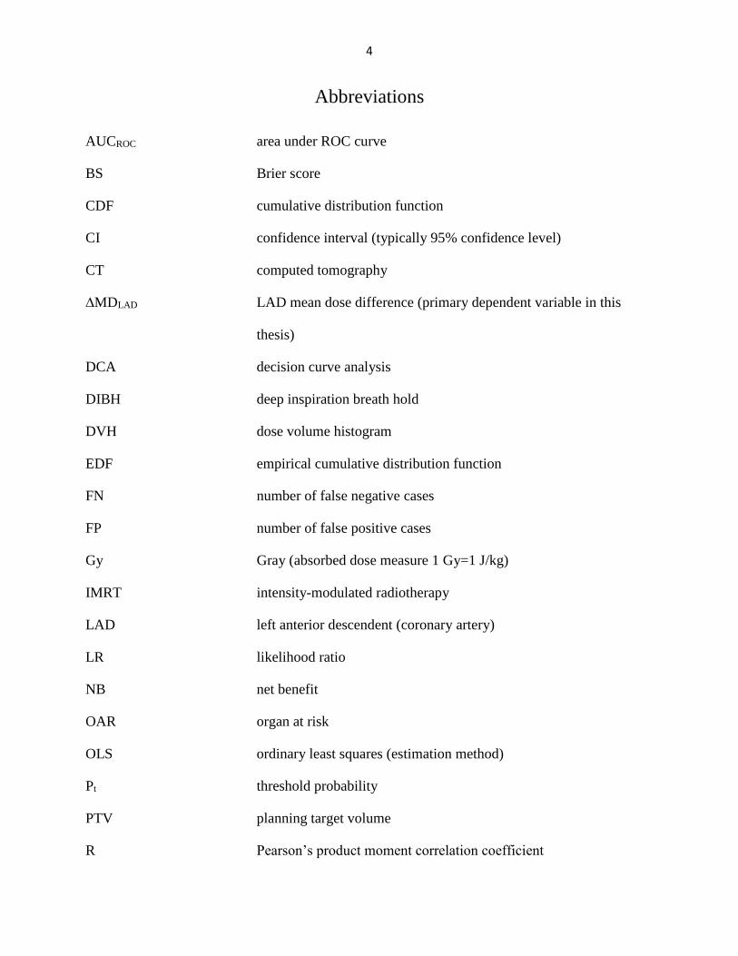
Estimated parameters and equation of the model
Estimated coefficient S.E. p
Area by DistanceMedianSupine -0.369 0.114 0.001
Area by BMI 0.033246 0.006764 <0.001
Constant -1.653 0.440 <0.001
Table 2. Estimated coefficients of the forward likelihood ratio selection logistic regression model.
A summary of the parameter estimates of this model is shown in Table 2. All parameters are
significant at the 1% level.
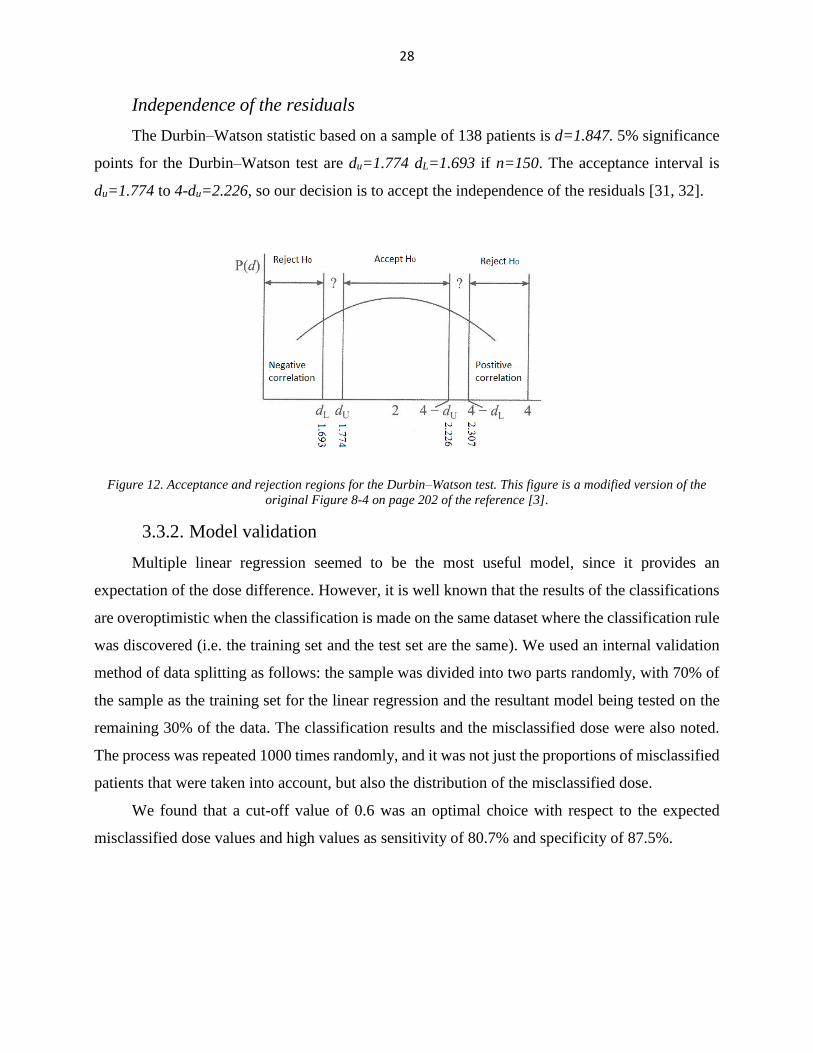
ROC analysis for the predicted probabilities
It can be seen in Figure 7 that the ROC curve is promisingly close to the ideal curve. AUCROC:
0.900 with standard error 0.027, 95% confidence interval for AUCROC: 0.848, 0.953.
Figure 7. ROC analysis results for the logistic regression of predicted probabilities. Non-hierarchical model.
3.3. Linear regression-based model
A serious weakness of logistic regression-based classification methods is that the dependent
variable is always binary. In our dataset, this would have led to a serious loss of information. The
dependent variable, LAD mean dose difference, is a continuous variable which is dichotomized by
its sign.
If we treat it as a continuous variable, the problem will be a ‘regression type’ problem. Higher
differences will be taken into account with more weight. The value of the LAD mean dose

24
difference is also expected. Knowledge of the expected dose difference is informative for physicists
and physicians involved in radiation treatment planning.
Estimated parameters of the model
Table 3 presents the estimated coefficients of the multiple linear regression.
Estimated
coefficient S.E. t-test statistic p
(Constant) -10.532 4.151 -2.537 0.012
DistanceMedianSupine -5.726 1.165 -4.917 <0.001
BMI 0.573 0.123 4.660 <0.001
Area_cm2 0.830 0.158 5.243 <0.001
Table 3. Estimated coefficients of the linear regression model.
Although standard errors of the parameter estimates were rather large, the fitted model was
useful for predictions. Almost all the coefficients of the fitted linear regression model are
significant at the 0.001 level (except the constant, which is significant at the 0.05 level).
Goodness of fit of the linear regression model
The goodness of fit of the model was examined with the following measures: the multivariate
correlation coefficient R=0.754 and the square of the adjusted multivariate correlation coefficient
R2adj=0.560.
ROC analysis for the linear regression model
It is also possible to apply ROC analysis to the linear regression model as well. We present
the result of the ROC analysis for the predicted values of the multiple linear regression model. Like
earlier logistic models, good results can be seen in Figure 8, where the ROC curve is promisingly
close to the ideal curve. AUCROC 0.903, 95% confidence interval for AUCROC: 0.850, 0.957.

25
Figure 8. ROC curve for the linear regression-based predicted values.
This result clearly shows that the regression-based method is useful for prediction.
A summary of the results of these methods is shown in Table 4.
Model AUC 95% Confidence interval for AUC Brier score
BMI (predictor only) 0.740 0.630, 0.850 0.201
Area (predictor only) 0.868 0.791, 0.944 0.151
Median distance (predictor only) 0.787 0.690, 0.884 0.189
Logistic regression (main effect model) 0.906 0.854, 0.959 0.124
Logistic regression (forward LR selection model) 0.900 0.848, 0.953 0.132
Linear regression 0.903 0.850, 0.957 0.139
Table 4. Primary classification results for the prediction models.
3.3.1. Model diagnostics for the linear regression model
Despite the promising results in the previous sections, it is crucial to investigate the
multivariate regression model in depth, especially to investigate the assumptions of the linear
regression model [3].
Distribution of the residuals
The normality of the residuals was checked graphically with a Q–Q plot and a histogram with
an estimated normal curve, which can be seen in Figure 9.

26
Figure 9. Distribution of the residuals: A. Histogram for the residuals with an estimated Gaussian (normal) density
curve; B. Q–Q plot for the residuals.
The Q–Q plot reveals no large deviations and no tendency in deviations. The linearity of the
points suggests that the residuals are normally distributed.
The Shapiro–Wilk test for normality confirms the result. The Shapiro–Wilk test results in a
p-value of p=0.592, which confirms that we have no reason to assume a different distribution than
normal.
Tendency of the residuals
The linear regression model assumes that the variance of the residuals is constant (see section
2.1.1.) The residuals might have an increasing (decreasing) or other kind of tendency in function
of the predicted values. The plot in Figure 10 clearly demonstrates that there is no overall trend for
the residuals, so the assumption of constant variance is fulfilled.

27
Figure 10. Scatter plot to present possible tendency of the residuals in function of the predicted value. The horizontal
axis shows predicted values, while the vertical axis represents residuals.
The plot for the residuals in the sequence of the data collected and the result is presented
below (Figure 11).
Figure 11. Scatter plot to present possible time-dependent tendency of the residuals. The horizontal axis shows the
ID numbers of the patients, while the vertical axis represents residuals.
It can be clearly seen that there is no overall time-dependent tendency at all.
28
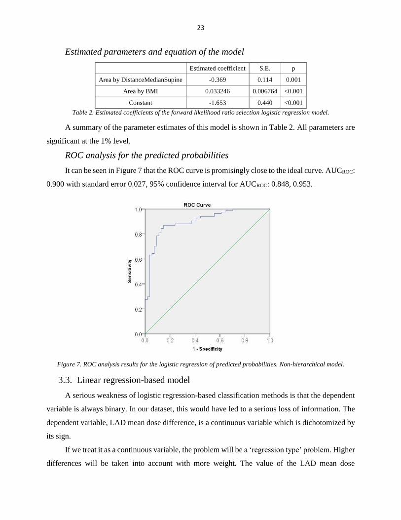
Independence of the residuals
The Durbin–Watson statistic based on a sample of 138 patients is d=1.847. 5% significance
points for the Durbin–Watson test are du=1.774 dL=1.693 if n=150. The acceptance interval is
du=1.774 to 4-du=2.226, so our decision is to accept the independence of the residuals [31, 32].
Figure 12. Acceptance and rejection regions for the Durbin–Watson test. This figure is a modified version of the
original Figure 8-4 on page 202 of the reference [3].
3.3.2. Model validation
Multiple linear regression seemed to be the most useful model, since it provides an
expectation of the dose difference. However, it is well known that the results of the classifications
are overoptimistic when the classification is made on the same dataset where the classification rule
was discovered (i.e. the training set and the test set are the same). We used an internal validation
method of data splitting as follows: the sample was divided into two parts randomly, with 70% of
the sample as the training set for the linear regression and the resultant model being tested on the
remaining 30% of the data. The classification results and the misclassified dose were also noted.
The process was repeated 1000 times randomly, and it was not just the proportions of misclassified
patients that were taken into account, but also the distribution of the misclassified dose.
We found that a cut-off value of 0.6 was an optimal choice with respect to the expected
misclassified dose values and high values as sensitivity of 80.7% and specificity of 87.5%.

29
Cut-off Sensitivity (%) Specificity (%)
Extent of wrong
estimate, decision:
prone (Gy,
mean±Sd)
Extent of wrong
estimate, decision:
supine (Gy,
mean±Sd)
-0.6 66.6 91.1 2.5±3.9 -0.7±1.0
-0.3 70.8 90.7 2.6±3.6 -0.8±1.1
0 74.4 90.0 2.4±3.4 -0.9±1.3
0.3 77.7 88.9 2.1±3.0 -1.2±1.6
0.6 80.7 87.5 1.7±2.6 -1.7±1.9
0.9 83.4 86.0 1.5±2.4 -2.0±2.2
1.2 85.4 83.6 1.1±2.3 -2.3±2.8
1.5 86.5 81.7 1.1±2.2 -3.0±3.7
1.8 86.8 79.9 1.3±2.3 -3.5±4.2
Table 5. Classification measures based on 1000 times random cross-validation. (We define supine position as
positive)
3.4. A few results on decision curves for ‘non-probability outcomes’
Our goal is to apply the decision curve method to linear regression-based predictions as well
as logistic regression-based predictions and compare our models with respect to net benefit values.
In the case of logistic regression models, the prediction is an expected probability; therefore, the
DCA can be applied directly. Linear regression results in an expected dose difference, so the
predicted value must be transformed into a range of probabilities.
The purpose of this section is to investigate how the shape of the decision curve depends on
the transformation function chosen and the probability distribution of this non-probability outcome.
These are unpublished results.
Although it is reasonable to use logistic regression to predict probabilities, there are other
plausible methods to solve this problem. In other words, there are several possible link functions
to transform the predicted scores or the expected values into probabilities. Plausible methods are,
for example, the use of the empirical cumulative distribution function (CDF) to obtain probabilities
or use an inverse logit link, probit link function or logistic regression-based probabilities.
These four transformations were chosen and examined for their effect on the shape of the
decision curve. Simulations were performed for the four transformations applied to symmetrical
and skewed probability distributions. The performance of the prediction naturally depends on the
shift of the groups, i.e. on the shift parameter between the two groups.

30
A very fundamental doubt is that the shape of the decision curve depends on the
transformation chosen. In this section, it will be confirmed that the shape of the decision curve
depends on the transformation (link function) chosen.
3.4.1. Simulation 1: The shape of the decision curve depends on the
transformation function chosen. Different continuous distributions
The first approach is the ‘regression type approach’. 10 000 random samples were simulated.
Random predictor (X) was simulated from different distributions: standard normal, uniform,
gamma and lognormal with the parameters noted below in formulae (14)...(17). We added random
residuals normally distributed with the parameters below. To construct a binary dependent variable,
a continuous dependent variable (Y) was first calculated as the sum of the predictor variable (X)
and the error term (ε).
10 000 random samples were simulated from normal (X1), uniform (X2), gamma (X3) and
lognormal (X4) distributions. The added random residuals (ε) were normally distributed with
mean=0 and SD=0.5. The four types of continuous dependent variables here are in (14), (15), (16)
and (17).
𝑌1 = 𝑋1 + 𝜀, 𝑋1~𝑁(0,1) and 𝜀~𝑁(0,0. 52) (14)
𝑌2 = 𝑋2 + 𝜀, 𝑋2~𝑈𝑛𝑖𝑓𝑜𝑟𝑚(−1,1) and 𝜀~𝑁(0,0. 52) (15)
𝑌3 = 𝑋3 + 𝜀, 𝑋3~𝐿𝑜𝑔𝑛𝑜𝑟𝑚𝑎𝑙(1,1) and 𝜀~𝑁(0,0. 52) (16)
𝑌4 = 𝑋4 + 𝜀, 𝑋4~𝐺𝑎𝑚𝑚𝑎(2,1) and 𝜀~𝑁(0,0. 52) (17)
where X has standard normal, uniform, gamma and lognormal distributions, respectively, ε
is the error term, ε has N(0,0.52) distribution, and X and ε are independent.
In the second step, two groups were formed to obtain binary dependent variables.
The continuous dependent variables (Y1…Y4) were cut at their median values to achieve a
binary response. For example, if the current value of Y1 exceeded the median value, then this case
was defined as positive; otherwise, it was defined as negative, and the ‘prevalence’ was therefore
0.5. Finally, the random predictors (X1...X4) were transformed into ‘probabilities’ using
probabilities predicted with empirical CDF (model 1), inverse logit link (model 2), probit function
(model 3) and logistic regression (model 4), and we constructed decision curves. The dependence
of the binary response on the random predictors (X1...X4) was also examined with ROC curves.
Results are shown in Figure 13. The area under the ROC curve shows a quite good separation
of the original predictors.
31
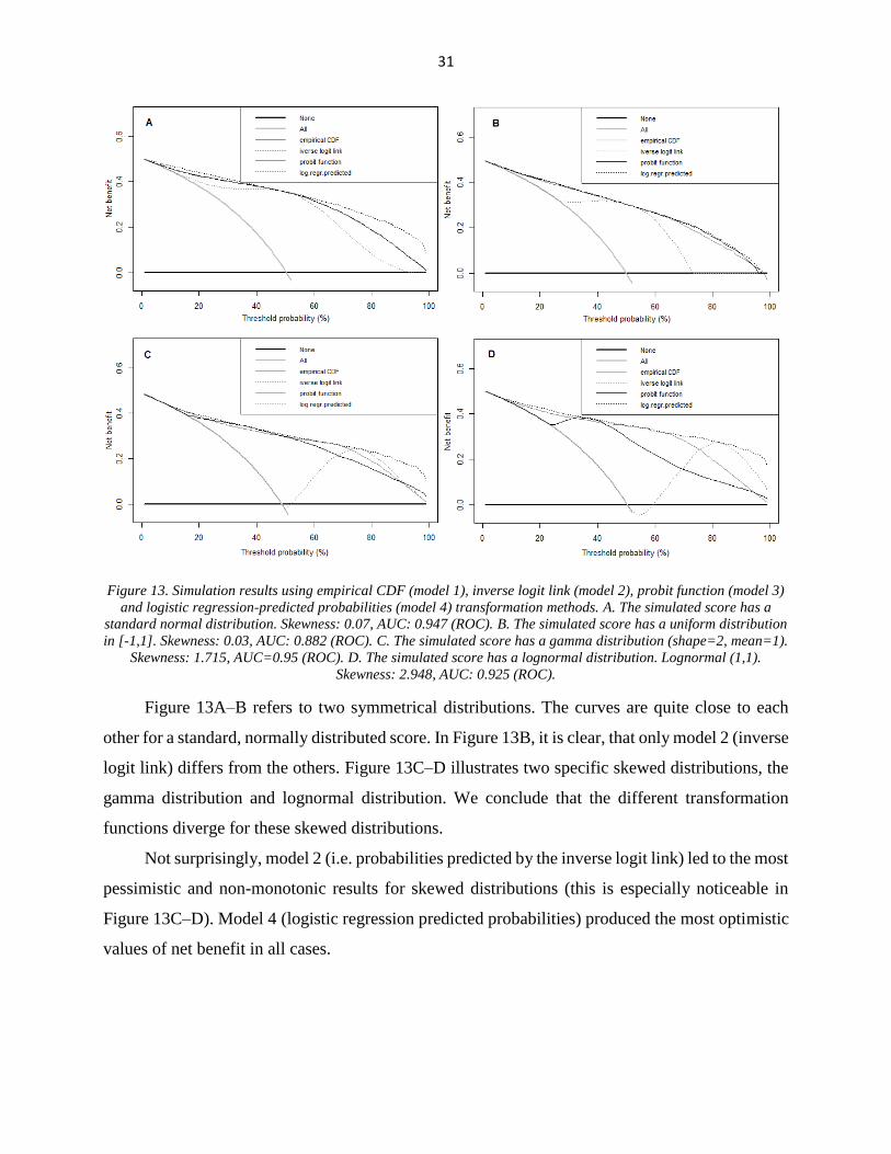
Figure 13. Simulation results using empirical CDF (model 1), inverse logit link (model 2), probit function (model 3)
and logistic regression-predicted probabilities (model 4) transformation methods. A. The simulated score has a
standard normal distribution. Skewness: 0.07, AUC: 0.947 (ROC). B. The simulated score has a uniform distribution
in [-1,1]. Skewness: 0.03, AUC: 0.882 (ROC). C. The simulated score has a gamma distribution (shape=2, mean=1).
Skewness: 1.715, AUC=0.95 (ROC). D. The simulated score has a lognormal distribution. Lognormal (1,1).
Skewness: 2.948, AUC: 0.925 (ROC).
Figure 13A–B refers to two symmetrical distributions. The curves are quite close to each
other for a standard, normally distributed score. In Figure 13B, it is clear, that only model 2 (inverse
logit link) differs from the others. Figure 13C–D illustrates two specific skewed distributions, the
gamma distribution and lognormal distribution. We conclude that the different transformation
functions diverge for these skewed distributions.
Not surprisingly, model 2 (i.e. probabilities predicted by the inverse logit link) led to the most
pessimistic and non-monotonic results for skewed distributions (this is especially noticeable in
Figure 13C–D). Model 4 (logistic regression predicted probabilities) produced the most optimistic
values of net benefit in all cases.

32
3.4.2. Simulation 2. The shape of the decision curve depends on the
transformation function chosen. Two normal distributions.
In this section, the simulated score has a standard normal distribution for group 0 (the non-
diseased or negative group) and different normal distributions (shifted) for group 1 (diseased or
positive). With this approach, we assume that the diseased group also has a normally distributed
score value, but with a different mean than the non-diseased group. The prevalence is 0.2. In this
section, the performance of the classification depends on the shift parameter between the normal
distributions.
10 000 random samples were simulated. The behaviour of the four transformation functions
was then examined. We conclude that empirical CDF (model 1), inverse logit link (model 2) and
probit function (model 3) lead to extremely low values of net benefit despite the very good
classification. This is especially noticeable in Figure 14D, where the shift parameter is 3SD
between the normal distributions, which represents a very good classification of the cases. Logistic
regression predicted probabilities produced the best values of net benefit as in section (3.4.1).
Results are shown in Figures 14A–D.

33
Figure 14. Simulation results, two normal distributions. Empirical CDF (model 1), inverse logit link (model 2),
probit function (model 3) and logistic regression predicted probabilities (model 4). A. The simulated score has a
standard normal distribution in the non-diseased group and a normal distribution with mean=0.33 and SD=1 in the
diseased group, AUC: 592 (ROC). B. The simulated score has a standard normal distribution in the non-diseased
group and a normal distribution with mean=0.5 and SD=1 in the diseased group, AUC: 0.639 (ROC). C. The
simulated score has a standard normal distribution in the non-diseased group and a normal distribution with
mean=1 and SD=1 in the diseased group, AUC: 0.762 (ROC). D. The simulated score has a standard normal
distribution in the non-diseased group and a normal distribution with mean=3 and SD=1 in the diseased group,
AUC: 0.983 (ROC).
It can be concluded based on these results that models 1–3, i.e. empirical CDF (model 1),
inverse logit link (model 2) and probit function (model 3), can lead to very low values of net benefit
even if the classification is very good and that these three transformation functions can bring about
very different results, especially for skewed distributions.
3.4.3. Conclusion about non-probability outcomes
Based on both approaches, we recommend the use of logistic regression-based probabilities
to construct the decision curve for ‘non-probability outcomes’. Our recommendation is the same
as in the R package by Vickers and Elkin [2]. We confirm that the most appropriate
transformation for such cases is logistic regression, which is used in the DecisionCurve and rmda
R packages [2, 33].

34
The decision curve method is applicable to continuous outcomes as well. There are two
approaches to this question.
Decision curves could be regarded as only applicable to probability expectations, and the
link function is part of the model that needs to be evaluated.
The link function could be regarded as part of the evaluation method, and the outcome of
the model is a score or continuous expected value.
These are two different aspects, but the conclusion is the same. We also recommend the use
of logistic regression-based probabilities to construct the decision curve for ‘non-probability
outcomes’.
3.5. Comparing our models using decision curves
The simulation results noted above allow us to evaluate the linear regression-based model
with respect to net benefit and DCA as well. The simulation results confirm the use of logistic
regression-predicted probabilities to construct decision curves for ‘non-probability outcomes’. We
examined the performance of the three best predictors alone with decision curves, and we compared
them to the models described in (3.2) and (3.3). None of the best three predictors alone was
comparable to the prediction models (Figure 15). For example, a univariate logistic regression was
applied with the independent variable BMI (and with the dependent variable preferable treatment
position, we defined supine as positive) to construct probability prediction based on the value of
BMI. In Figure 15 ‘all’ refers to ‘all positive’ (i.e. all patients treated in the supine position) and
‘none’ indicates ‘all negative’ (i.e. all patients treated in the prone position).
In our analyses, decision curves for both the logistic regression model and the linear
regression-based model were quite similar to each other; additionally, it is important that both
models led to high values of net benefit for a wide range of threshold probabilities. In other words,
it is beneficial to use these models in respect of net benefit regardless of the current threshold
probability. These results showed that these models can be used in clinical practice.

35
Figure 15. Decision curves for the three best predictors and three models. Model 1 refers to the predictor BMI,
model 2 to the predictor area, and model 3 to the predictor median distance; model 4 and model 5 are logistic
regression-based models. Model 4 is the main effect model (area+BMI+median distance), model 5 is the forward
likelihood ratio selection model, with two interaction terms (area*BMI+area*median distance), and model 6 is the
linear regression-based model.
A bootstrap method was applied to construct 95% confidence intervals for the net benefit at
various threshold levels for the main effect model. 10 000 bootstrap samples of sample size 138
were generated by Microsoft Excel. Net benefit values were calculated by definition. The 2.5%
and 97.5% percentiles of the net benefit values were calculated at each threshold level. The results
are shown in Table 6.
Threshold probability Lower bound for net benefit Upper bound for net benefit
0.1 0.564 0.573
0.2 0.496 0.547
0.3 0.450 0.527
0.4 0.423 0.517
0.5 0.391 0.507
0.6 0.319 0.467
0.7 0.256 0.435
0.8 0.210 0.435
0.9 0.000 0.333
Table 6. 95% confidence intervals for net benefit (logistic regression, main effect model) at different threshold levels.
Confidence bounds are based on 1000 bootstrap samples.

36
The differences between the logistic regression models and the multiple regression-based
model are not relevant with respect to the very similar net benefit values. All of these models led
to high values of net benefit for a wide range of possible threshold levels.
3.6. Predictor error consequences and further testing on an independent dataset
of patients
In all of the previous sections, we assumed that there are no predictor errors at all. This was
quite plausible because a series of CT scans can provide a precise way to measure the predictor
values. In this section, we introduce the predictor values based on only one CT slice. It is very
reasonable to assume that predictor values based on only one CT slice might be affected by
measurement errors.
In this section, we would like to reach two of our goals. First is the investigation of possible
predictor errors, and second is the testing of the linear regression-based model in the data for 100
more patients. We found it very important to examine the possible predictor measurement errors.
The selection of the single CT slice might have an effect on predictor values. This phenomenon
can be called a ‘plane miss’.
The author of this thesis is not an expert in CT methodology and treatment planning methods.
The selection method of the single CT slice and the ‘plane miss’ phenomenon is described in detail
in [26, 34].
At this stage (we can call it stage 3, see the description in the data section (2.3.1)), our linear
regression-based model was intended to use the predictor values area and median distance based
on only one CT slice.
If this model works well, a ‘calculator’ can be prepared to aid physicians in decision-making
in their practice [26].
Before everyday use of the calculator, it is essentially important to investigate these errors
and especially investigate their consequences in the prediction [26].

37
3.6.1. Predictor errors
The predictor errors for area and median distance are evaluated here. These predictors were
measured on the CT series (as a reference) and based on only one CT slice in the sample of 100
patients. This provides the opportunity to compare the values.
Bland–Altman plots were used for comparison; they can be found in Figure 16. 95% limits
of agreement are -5.624 cm2 to 3.902 cm2 for the predictor area and -0.829 cm to 0.783 cm for the
predictor median distance.
Figure 16. Bland–Altman plots for predictor error evaluation. A refers to the predictor area, and B illustrates the
predictor median distance. The horizontal axis represents the average for the two different measures (i.e. the CT
series vs. one CT slice), while the vertical axis shows the difference between the two measures. The red lines refer to
95% limits of agreement.
Although these predictor errors are reasonably high, we will see that the effect on the
predictions is not critical.

38
3.6.2. Effect of predictor errors in the final prediction
First, the Bland–Altman plot for the predicted values will be presented. Here we calculated
the predicted values with our ‘calculator’ (i.e. the linear regression-based model) based on the
predictor values from only one CT slice and based on the predictor values from the CT series.
Figure 17. Bland–Altman plots for prediction error evaluation. This figure compares the predictions of the linear
regression-based model (i.e. ‘calculator’) based on only one CT slice and a series of CT slices. The horizontal axis
represents the average of the predictions, while the vertical axis shows the difference between the two predictions.
Red lines refer to 95% limits of agreement.
95% limits of agreement are -6.65 Gy to 7.82 Gy. These limits define quite a long interval.
The Bland–Altman plot seems to be the most important graphic method to show agreement
between two measures [27, 35]. However, here our goal is prediction, and Figure 18 below is at
least as important as the Bland–Altman plot was. Figure 18A shows a comparison of predictions
based on a series of CT slices and based on only one CT slice, and this is equivalent to Figure 17
above, but in Figure 18B the horizontal axis refers to the prediction based on only one CT slice and
the vertical axis presents the DVH data (from radiation treatment plans). DVH data is regarded as
the gold standard to ascertain the real LAD dose difference.

39
Figure 18. Comparison of predictions. A. Linear regression-based predictions based on a single CT scan (horizontal
axis) vs. linear regression-based predictions based on a series of CT scans (vertical axis). B. Doses according to the
estimation of the simple clinical method (linear regression) based on a single CT scan (horizontal axis) vs. DVH
data (gold standard) extracted from the planning system (vertical axis). Dashed lines indicate cut-off values of 0.6
Gy. [26]
Although the Bland–Altman limits of agreement were reasonably wide, Figure 18B is
promising and most of the points are located in the 1st and 3rd quadrants, suggesting that a large
portion of the predictions will be correct as well. Table 7 contains the validation data, and it is
important to compare the second and third columns of this table to the last two. This table clearly
demonstrates that the effect of possible predictor measurement errors is not crucial in our simple
predictive tool [9].
Original patient data (double CT method)
cross-validation results
Using predictors based on only one CT
slice
Cut-off Sensitivity (%) Specificity (%) Sensitivity (%) Specificity (%)
-0.6 66.6 91.1 72.4 91.5
-0.3 70.8 90.7 75.9 91.5
0 74.4 90.0 75.9 91.5
0.3 77.7 88.9 79.3 88.7
0.6 80.7 87.5 82.8 87.3
0.9 83.4 86.0 82.8 83.1
1.2 85.4 83.6 86.2 81.7
1.5 86.5 81.7 86.2 77.5
1.8 86.8 79.9 93.1 76.1
Table 7. Classification measures for ∆MDLAD using a single discrimination threshold. Great consistency is seen
between the original cohort and the present series [26].
40
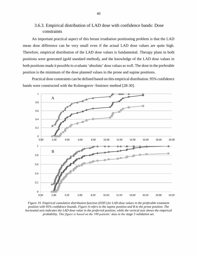
3.6.3. Empirical distribution of LAD dose with confidence bands: Dose
constraints
An important practical aspect of this breast irradiation positioning problem is that the LAD
mean dose difference can be very small even if the actual LAD dose values are quite high.
Therefore, empirical distribution of the LAD dose values is fundamental. Therapy plans in both
positions were generated (gold standard method), and the knowledge of the LAD dose values in
both positions made it possible to evaluate ‘absolute’ dose values as well. The dose in the preferable
position is the minimum of the dose planned values in the prone and supine positions.
Practical dose constraints can be defined based on this empirical distribution. 95% confidence
bands were constructed with the Kolmogorov–Smirnov method [28-30].
Figure 19. Empirical cumulative distribution function (EDF) for LAD dose values in the preferable treatment
position with 95% confidence bounds. Figure A refers to the supine position and B to the prone position. The
horizontal axis indicates the LAD dose value in the preferred position, while the vertical axis shows the empirical
probability. This figure is based on the 100 patients’ data in the stage 3 validation set.
-0.2
0
0.2
0.4
0.6
0.8
1
0.00 2.00 4.00 6.00 8.00 10.00 12.00 14.00 16.00 18.00 20.00
A
B

41
Dose constraints were defined based on the empirical distribution and based on medical
considerations. We agreed on the use of the 90% percentile of the EDF of the dose values. Our
estimates were 12.5 Gy and 12.9 Gy in the supine and prone positions, respectively [26].
Although Kolmogorov–Smirnov confidence bounds are reasonably wide, in the supine
position even the lower bound of the 95% confidence band is close to 70% at the point of 12.5 Gy.
This means that it is very unlikely that more than 30% of the cases in the future will exceed this
value. In prone position the lower bound of the 95% confidence band is also around 70% at 12.9
Gy, so the conclusion is very similar; it is also very unlikely that more than 30% of the patients
will exceed this 12.9 Gy value in the prone position.
We determined dose constraints based on the empirical distribution of the dose values in the
preferable position in the last section. We regarded these dose constraints as reasonable bounds
above which another kind of intervention is needed. This other kind of intervention may be
treatment planning in the other position or application of other radiation therapy techniques, such
as IMRT (intensity-modulated radiotherapy) [26].
3.6.4. External testing of the model
The validation process can be divided into three different steps [9]. The results of the random
cross-validation can be regarded as ‘internal validation’ [24, 25]. The classification results for the
additional 100 patients’ data and the results based on a single CT slice can be considered as a
‘temporal validation’ because the data was derived from the same centre at a later time. External
validation is needed to present generalizability of the model. One successful step was the external
testing of our linear regression-based model. It was tested in a 28-case dataset of left-side breast
cancer patients from Liège and showed great consistency with our results noted above. The
predicted treatment position was correct in 24/28 (accuracy: 85.7%) cases [26, 34].

42
4. Discussion
Therapeutic prediction models were developed and evaluated in our interdisciplinary study.
These models were based on well-established medical statistical methods, such as linear regression
and logistic regression [1, 36-39].
The mathematical aspects of the evaluation of the predictive power of these models were
presented in detail. The novel method of decision curves was used to compare these models.
Simulations were carried out to clarify how the DCA can be performed on ‘non-probability
outcomes’, such as scores or expected dose values. An evaluation of the predictive model was
presented in detail. The widely accepted method of cross-validation was used for internal
validation. Temporal validation and investigation of the possible predictor errors were carried out
using an additional dataset of patients. The oft-cited method developed by the two great Russian
mathematicians, Kolmogorov and Smirnov [28-30], was applied to construct a confidence band for
the empirical cumulative distribution of the dose values. This method was used to determine dose
constraints.
None of the single predictors alone was satisfactory for prediction. All the predictive models
performed better than single predictors did. The linear regression model was considered the most
clinically relevant for quantitative estimation, since it provides an estimate for dose difference and
is comparable to the two logistic regression models in all other aspects. DCA demonstrated very
similar performance, and AUCROC was almost the same for both the linear regression model and
the logistic regression-based models. Validation steps confirmed that the model is stable. The
Kolmogorov–Smirnov method showed that it is very likely (i.e. there is a 95% chance) that less
than 30% of patients exceed the dose constraints we defined.
Strengths and weaknesses of the study
It is very important to minimize OAR radiation doses with individual positioning. The linear
regression-based tool estimates the difference in the expected dose values based on the BMI and
the dmedian and Aheart measured on a CT slice at the middle of the heart. The result was compared to
that of the full CT series in both positions and the dosimetric data. The comparison between the
linear regression-based tool (based on only one CT slice) and the original method (predictors based
on series of CT-scans) found very consistent results (very similar sensitivity and specificity values)
[26]. This linear regression-based model and the calculator can be used in everyday practice as a
useful tool to aid in radiation treatment planning.

43
One strength of our study is its relatively large sample size and multivariate aspect. Decision
curves and the AUC for the ROC results were found to be similar for the linear regression model
and the two logistic regression models [25]. The logistic regression models weight the outcomes
on a binary scale, while the linear regression model weights them in keeping with the magnitude
of the difference, which we regarded as a great advantage for practical aspects. Since the linear
regression model provides additional information, i.e. an estimate of the dose difference, we
decided to use the linear regression model. Knowledge of the estimated quantitative benefit of one
or the other treatment position during radiotherapy may provide better guidance for the physician
when considering various aspects, such as repositioning accuracy and patient comfort.
Applying AUCROC and measures like sensitivity and specificity is very common in
radiotherapy planning, but we have not seen the approach of using decision curves in this field.
Our investigations point to the clinical utility of predictive models. The methodology described in
this thesis might be adapted for decision-making problems in other areas of medicine.
This investigation has its own limitations. One limitation might be that we assumed a linear
relationship between the predictors and the dependent variable. It can be seen in the scatter plots
that the data is dispersed and the data shows no other clear tendency or pattern. Further
investigations have found that none of the higher-order terms (squares or cubes of the predictors)
improved the model. A linear relationship may be a target of criticism, but we found no other
simple relationship more suitable for model building.
At the beginning of our investigations, predictor values were based on a series of CT slices.
Even these predictor values may be affected by measurement errors. In this investigation, we did
not have the opportunity to perform repeated measures or to set the predictor values to investigate
the effect of predictor measurement errors. The use of the OLS (ordinary least squares) estimation
(to estimate model coefficients) might be criticised, but the assumptions of the linear regression
model were checked carefully and the residual plot demonstrated no connection between the
variance of the dependent variable and the predictor values. Residual plots are also of great
importance to evaluate the goodness of fit of the model used [39].
Predictor values based on only one CT slice are measured with supposedly larger errors. At
this stage, the predictors were measured both ways (i.e. based on a series of CT slices and based
on only one CT slice). This design allowed us to evaluate the predictor errors based on only one
CT slice and to evaluate the consequences in a sample of 100 patients.

44
There are certain limitations of the linear regression model. The performance of the model is
fair, but limited to a sensitivity of 80.7% and a specificity of 87.5%. These values seemed to be
stable throughout the different steps of the evaluation [26].
Comparison with other studies in the context of other heart-sparing methods
There is a strong effort to minimize OAR doses during radiation therapy.
As an initial approach, in Lymberis et al., a Spearman correlation analysis was applied to
identify a monotonic relationship between OAR dose values and in-field OAR volumes [40]. At
present, the risk of radiogenic heart sequelae is thought to be related to the mean dose to the heart
[41, 42]. Based on epidemiological data and the simulation of out-of-date techniques, the mean
heart dose is a good approximation; however, many centres also focus on the dose to the coronary
arteries, most significantly the LAD. We believe that the LAD dose is a rational measure of the
danger to the heart in left-sided cases [41, 43-45].
Our LAD dose constraints (i.e. 12.5 Gy and 12.9 Gy in the supine and prone positions,
respectively) can be regarded as low and strict dose values compared to Jacob et al. [46].
Zhao at el. built an SVM (support vector machine)-based two-step decision-making
algorithm in a sample of 198 patients [47]. Their method is based on anatomical characteristics
measured on a prone CT series. The outcome of that test decides whether the patient benefits from
the prone position radiotherapy or should undergo a CT series in the supine position for
comparison. Although numerical measures of the goodness of classification were impressive, that
tool provided no numerical estimate of the advantage of one treatment position over the other;
hence, no optimization could be practised. With the SVM method, the selection of cases with an
in-field heart volume over the acceptable threshold in the prone position could be managed, and in
some cases, a second CT series was needed in the supine position. Furthermore, no volumetric dose
data could be collected [47].
Another potential method to minimize OAR dose values is the use of the deep inspiration
breath hold technique (DIBH). Lin et al. compared the DIBH method and prone positioning [48].
Their results demonstrate that it is rather difficult to distinguish patients who benefit from DIBH
versus patients who have benefited from prone positioning. Although the mathematical and IT
apparatus they used is impressive, their results were based on a relatively small sample of 16
patients and therefore their results might be rather limited.

45
Recently, the optimal use of prone and supine positioning vs. other kinds of techniques
(such as DIBH and IMRT) has become a topic of intensive research. The results of Lin et. al suggest
that the classification problem (that is, predicting the best intervention method) can be statistically
very challenging [48].
Recommendations for clinical practice
Although this thesis has discussed the use of the LAD mean dose difference in detail as a
primary outcome, there are other possible dependent variables, such as the heart dose. In clinical
practice, an algorithm for the dose to the heart is also considered in a complex decision, but only
as a secondary outcome measure [26]. In most centres, the most widely applied outcome measure
is the mean heart dose [42, 49]. Since a linear, non-threshold association exists between the mean
heart dose and coronary events, the mean heart dose may be regarded as an approximation of the
doses to the LAD and other coronary arteries [49].
Since there is a strong correlation between mean heart dose and LAD dose (R=0.87 in both
positions), we believe that the predictive model presented here could be adapted to local practice
after careful investigation in any centre applying prone radiotherapy.
Moreover, the simple tool, which uses a single CT slice in the supine position, combined
with the dose constraints described in [26] is in everyday use at the Department of Oncotherapy,
University of Szeged. The linear regression-based model was also tested in a 28-case external
dataset of left-side breast cancer patients from Liège and showed great consistency in our results
noted above. Predicted treatment position was correct in 24 out of 28 (accuracy: 85.7%) cases [26].

46
5. Summary and new results
Decision curves proved to be useful in comparing our models. We consider the linear
regression model as a useful tool to support physicists and physicians in predicting the preferable
treatment position. These results are promising and show that these predictive models can be used
effectively in everyday clinical practice with the dose constraints described. The linear regression-
based calculator is in use at the University of Szeged Department of Oncotherapy.
Our results identified a relation between the predictors (BMI, median distance and area)
and the LAD mean dose difference.
The multiple linear regression-based model was developed and has proved to be an
effective prediction model for the selection of the optimal radiation therapy position of
left breast cancer patients.
It was shown that the application of decision curve analysis for ‘non-probability
outcomes’ is effective. Our simulation results confirm the use of logistic regression to
produce probabilities to calculate ‘net benefit’.
The novel decision curve method has been effectively applied to evaluate the performance
of this multiple linear regression model.
The decision curve analysis and the random cross validation method clearly present the
effectiveness of the multiple linear regression model.
The multiple regression-based model is applied in everyday medical practice (under well-
defined dose constraints) at the University of Szeged Department of Oncotherapy [26].
The multiple regression-based model is applicable to predict preferable treatment
position.

47
Acknowledgements
I am greatly obliged to Dr. Krisztina Boda and to Professor Tibor Nyári, my supervisors, for
their continuous support and guidance in my scientific activities.
I am deeply indebted to Professor Zsuzsanna Kahán, former director of the Department of
Oncotherapy, for her continuous optimism and immensely supportive encouragement.
I am very grateful to Dr. Renáta Lilla Kószó and Dr. Zoltán Varga (Department of
Oncotherapy) for providing me with the opportunity to collaborate with them.
I also wish to thank all my co-authors for the chance to work with them.
I would like to express my gratitude to Professor Ferenc Bari and Professor Ferenc Peták,
former and current heads of the Department of Medical Physics and Informatics, for providing me
with the facilities necessary to complete this thesis and for their continuous kind support.
Thanks as well to all my colleagues at the Department of Medical Physics for being so
friendly and supportive.
I am very grateful to Dr. Thomas Williams for his thoroughgoing work in reviewing the
language of the thesis.
I would like to express my appreciation to my teachers and professors in the past for their
conscientious work in educating me.
I wish to thank all my friends for their kind, supportive attitude.
I am especially thankful to my parents and my family for their never-ending supportive
attitude and for their enormous encouragement.
With this dissertation, I would like to thank my parents in particular for their emotional and
financial support throughout my studies and for the fact that they have always believed in me.
This research was partly supported by the European Union and the State of Hungary, co-
financed by the European Social Fund within the framework of EFOP-3.6.1-16-2016-00008.

48
References
1. Tripepi, G., et al., How to deal with continuous and dichotomic outcomes in
epidemiological research: linear and logistic regression analyses. Nephron Clin Pract,
2011. 118(4): p. c399-406.
2. Vickers, A.J. and E.B. Elkin, Decision curve analysis: a novel method for evaluating
prediction models. Med Decis Making, 2006. 26(6): p. 565-74.
3. Kemény, S., et al., Kísérletek tervezése és értékelése. 2017, Budapest: Typotex.
4. Rawlings, J.O., S.G. Pantula, and D.A. Dickey, Applied regression analysis : a research
tool. 2nd ed. Springer texts in statistics. 1998, New York: Springer. xviii, 657 p.
5. Draper, N.R. and H. Smith, Applied regression analysis. 3rd ed. Wiley series in probability
and statistics Texts and references section. 1998, New York: Wiley. xvii, 706 p.
6. Montgomery, D.C. and G.C. Runger, Applied statistics and probability for engineers. 3rd
ed. 2003, New York: Wiley. xiv, 706 p.
7. Stoltzfus, J.C., Logistic regression: a brief primer. Acad Emerg Med, 2011. 18(10): p.
1099-104.
8. Hosmer, D.W. and S. Lemeshow, Applied logistic regression. 2nd ed. Wiley series in
probability and statistics Texts and references section. 2000, New York: Wiley. xii, 373 p.
9. Altman, D.G. and P. Royston, What do we mean by validating a prognostic model? Stat
Med, 2000. 19(4): p. 453-73.
10. Agresti, A., Categorical data analysis. 2nd ed. Wiley series in probability and statistics.
2002, New York: Wiley-Interscience. xv, 710 p.
11. Baker, S.G. and B.S. Kramer, Peirce, Youden, and Receiver Operating Characteristic
Curves. The American Statistician, 2007. 61(4): p. 343-346.
12. López-Ratón, M., et al., OptimalCutpoints: An R Package for Selecting Optimal Cutpoints
in Diagnostic Tests. Journal of Statistical Software; Vol 1, Issue 8 (2014), 2014.
13. Obuchowski, N.A., M.L. Lieber, and F.H. Wians, Jr., ROC curves in clinical chemistry:
uses, misuses, and possible solutions. Clin Chem, 2004. 50(7): p. 1118-25.
14. Steyerberg, E.W., et al., Graphical assessment of incremental value of novel markers in
prediction models: From statistical to decision analytical perspectives. Biom J, 2015.
57(4): p. 556-70.
15. BRIER, G.W., VERIFICATION OF FORECASTS EXPRESSED IN TERMS OF
PROBABILITY. Monthly Weather Review, 1950. 78(1): p. 1-3.
16. Augustin, H., et al., Decision curve analysis to compare 3 versions of Partin Tables to
predict final pathologic stage. Urol Oncol, 2012. 30(4): p. 396-401.
17. Collins, G.S. and D.G. Altman, Predicting the 10 year risk of cardiovascular disease in the
United Kingdom: independent and external validation of an updated version of QRISK2.
BMJ, 2012. 344: p. e4181.

49
18. Godoy, G., et al., Extent of pelvic lymph node dissection and the impact of standard
template dissection on nomogram prediction of lymph node involvement. Eur Urol, 2011.
60(2): p. 195-201.
19. Lughezzani, G., et al., Comparison of three different tools for prediction of seminal vesicle
invasion at radical prostatectomy. Eur Urol, 2012. 62(4): p. 590-6.
20. Steyerberg, E.W., et al., Assessing the performance of prediction models: a framework for
traditional and novel measures. Epidemiology, 2010. 21(1): p. 128-38.
21. Ankerst, D.P., et al., Updating risk prediction tools: a case study in prostate cancer. Biom
J, 2012. 54(1): p. 127-42.
22. Barbieri, C.E., et al., Decision curve analysis assessing the clinical benefit of NMP22 in the
detection of bladder cancer: secondary analysis of a prospective trial. BJU Int, 2012.
109(5): p. 685-90.
23. Peirce, C.S., The numerical measure of the success of predictions. Science, 1884. 4(93): p.
453-4.
24. Varga, Z., et al., Individualized positioning for maximum heart protection during breast
irradiation. Acta Oncol, 2014. 53(1): p. 58-64.
25. Rarosi, F., et al., Decision curve analysis apropos of choice of preferable treatment
positioning during breast irradiation. BMC Med Inform Decis Mak, 2019. 19(1): p. 204.
26. Kahan, Z., et al., A simple clinical method for predicting the benefit of prone vs. supine
positioning in reducing heart exposure during left breast radiotherapy. Radiother Oncol,
2018. 126(3): p. 487-492.
27. Bland, J.M. and D.G. Altman, Statistical methods for assessing agreement between two
methods of clinical measurement. Lancet, 1986. 1(8476): p. 307-10.
28. Kolmogorov, A.N., Sulla determinazione empirica di una legge di distribuzione. Giorn. Ist.
Ital. Attuari, 1933(4): p. 83-91.
29. Kolmogorov, A.N., Confidence Limits for an Unknown Distribution Function. Ann. Math.
Statist., 1941. 12(4): p. 461-463.
30. Smirnov, N.V., Tables for estimating the goodness of fit of empirical distributions. Annals
of Mathematical Statistics, 1948. 19: p. 279-281.
31. Durbin, J. and G.S. Watson, Testing for serial correlation in least squares regression. I.
Biometrika, 1950. 37(3-4): p. 409-28.
32. Durbin, J. and G.S. Watson, Testing for serial correlation in least squares regression. II.
Biometrika, 1951. 38(1-2): p. 159-78.
33. Vickers, A.J. Decision curve analysis. [homepage] 2010; [program packages]. Available
from: www.decisioncurveanalysis.org.
34. Kószó, R.L., Individualised radiotherapy serving reducedtoxicityin breast and prostate
cancer, in Doctoral School of Interdisciplinary Sciences, Faculty of Medicine, University
of Szeged, Hungary. 2018, University of Szeged: Szeged.
35. Bland, J.M. and D.J. Altman, Regression analysis. Lancet, 1986. 1(8486): p. 908-9.

50
36. Kasza, J. and R. Wolfe, Interpretation of commonly used statistical regression models.
Respirology, 2014. 19(1): p. 14-21.
37. Lee, K.J., M.M. Wiest, and J.B. Carlin, Statistics for clinicians: an introduction to linear
regression. J Paediatr Child Health, 2014. 50(12): p. 940-3.
38. Schneider, A., G. Hommel, and M. Blettner, Linear regression analysis: part 14 of a series
on evaluation of scientific publications. Dtsch Arztebl Int, 2010. 107(44): p. 776-82.
39. Godfrey, K., Simple linear regression in medical research. N Engl J Med, 1985. 313(26):
p. 1629-36.
40. Lymberis, S.C., et al., Prospective assessment of optimal individual position (prone versus
supine) for breast radiotherapy: volumetric and dosimetric correlations in 100 patients. Int
J Radiat Oncol Biol Phys, 2012. 84(4): p. 902-9.
41. Darby, S.C., et al., Risk of ischemic heart disease in women after radiotherapy for breast
cancer. N Engl J Med, 2013. 368(11): p. 987-98.
42. Kirby, A.M., et al., Prone versus supine positioning for whole and partial-breast
radiotherapy: a comparison of non-target tissue dosimetry. Radiother Oncol, 2010. 96(2):
p. 178-84.
43. Taylor, C.W. and A.M. Kirby, Cardiac Side-effects From Breast Cancer Radiotherapy.
Clin Oncol (R Coll Radiol), 2015. 27(11): p. 621-9.
44. Taylor, C.W., et al., Exposure of the Heart in Breast Cancer Radiation Therapy: A
Systematic Review of Heart Doses Published During 2003 to 2013. Int J Radiat Oncol Biol
Phys, 2015. 93(4): p. 845-53.
45. Duane, F.K., et al., Cardiac Structure Doses in Women Irradiated for Breast Cancer in the
Past and Their Use in Epidemiological Studies. Pract Radiat Oncol, 2019. 9(3): p. 158-171.
46. Jacob, S., et al., Is mean heart dose a relevant surrogate parameter of left ventricle and
coronary arteries exposure during breast cancer radiotherapy: a dosimetric evaluation
based on individually-determined radiation dose (BACCARAT study). Radiat Oncol, 2019.
14(1): p. 29.
47. Zhao, X., et al., A support vector machine (SVM) for predicting preferred treatment position
in radiotherapy of patients with breast cancer. Med Phys, 2010. 37(10): p. 5341-50.
48. Lin, H., et al., Feasibility study of individualized optimal positioning selection for left-sided
whole breast radiotherapy: DIBH or prone. J Appl Clin Med Phys, 2018. 19(2): p. 218-
229.
49. Wurschmidt, F., et al., Incidental dose to coronary arteries is higher in prone than in supine
whole breast irradiation. A dosimetric comparison in adjuvant radiotherapy of early stage
breast cancer. Strahlenther Onkol, 2014. 190(6): p. 563-8.


I. Rárosi, F., Boda, K., Kahán, Z., and Varga, Z. (2019). Decision curve
analysis apropos of choice of preferable treatment positioning during
breast irradiation. BMC Medical Informatics and Decision Making 19(1),
204. IF: 2.067

RESEARCH ARTICLE Open Access
Decision curve analysis apropos of choiceof preferable treatment positioning duringbreast irradiationFerenc Rárosi1* , Krisztina Boda1, Zsuzsanna Kahán2 and Zoltán Varga2
Abstract
Background: Radiotherapy is a standard treatment option for breast cancer, but it may lead to significant latemorbidity, including radiation heart damage. Breast irradiation performed individually in the supine or proneposition may aid in minimizing the irradiation dose to the heart and LAD coronary artery. A series of CT scans andtherapy plans are needed in both positions for the ‘gold standard’ decision on the preferable treatment position.This method is expensive with respect to technology and physician workload.Our ultimate goal is to develop a predictive tool to identify the preferable treatment position using easilymeasurable patient characteristics. In this article, we describe the details of how model building and consequentlyvalidation of the best model are done.
Methods: Different models were used: both logistic regression and multiple linear regressions were used toestimate the LAD mean dose difference (the difference between the mean dose to the LAD in the supine positionversus prone position); predicted dose differences were analysed compared to the ‘gold standard’ values, and thebest model was selected accordingly. The final model was checked by random cross-validation. In addition togenerally used measures (ROC and Brier score), decision curves were employed to evaluate the performance of themodels.
Results: ROC analysis demonstrated that none of the predictors alone was satisfactory. Multiple logistic regressionmodels and the linear regression model lead to high values of net benefit for a wide range of thresholdprobabilities. Multiple linear regression seemed to be the most useful model. We also present the results of therandom cross-validation for this model (i.e. sensitivity of 80.7% and specificity of 87.5%).
Conclusions: Decision curves proved to be useful to evaluate our models. Our results indicate that any of themodels could be implemented in clinical practice, but the linear regression model is the most useful model tofacilitate the radiation treatment decision. In addition, it is in use in everyday practice in the Department ofOncotherapy, University of Szeged, Hungary.
Keywords: Decision curve, Regression model, Prediction, Validation, Left-sided breast radiotherapy, LAD mean dose
© The Author(s). 2019 Open Access This article is distributed under the terms of the Creative Commons Attribution 4.0International License (http://creativecommons.org/licenses/by/4.0/), which permits unrestricted use, distribution, andreproduction in any medium, provided you give appropriate credit to the original author(s) and the source, provide a link tothe Creative Commons license, and indicate if changes were made. The Creative Commons Public Domain Dedication waiver(http://creativecommons.org/publicdomain/zero/1.0/) applies to the data made available in this article, unless otherwise stated.
* Correspondence: [email protected] of Medical Physics and Informatics, University of Szeged,Korányi fasor 9, Szeged 6720, HungaryFull list of author information is available at the end of the article
Rárosi et al. BMC Medical Informatics and Decision Making (2019) 19:204 https://doi.org/10.1186/s12911-019-0927-4

BackgroundRadiotherapy is an effective treatment for breast cancer,but it can lead to significant late morbidity, particularlyconnected to various heart diseases [1, 2]. The goal ofradiotherapy is to achieve a good therapeutic ratio, i.e. asufficient dose in the planning target volume but as lowas possible to normal tissues and especially to critical or-gans at risk (OAR). Great efforts are made to minimizethe irradiation dose to the heart in general; nevertheless,the dose to the LAD is of the utmost clinical importance[3]. There are different approaches to protect the heartfrom radiation, among which breathing control, includ-ing the deep inspirational breast hold technique andIMRT or partial breast irradiation, have just recently be-come available in routine practice [4, 5]. Originally,prone positioning was invented for the irradiation of dif-ficult cases with large breasts, and many groups came tofavour its wide use [6–11]. Numerous studies includingours have demonstrated that the preferable position var-ies from patient to patient [6–8, 12–16]. Some investiga-tions have identified patient-related predictors in favourof a particular treatment position, while others have not.There are studies that prefer the prone position for
heart protection in general; others did not find a relevantbenefit of prone positioning compared to supine posi-tioning [8, 16]. Investigations have demonstrated that thefavourable treatment set-up varies from patient to patientbut have not shown patient-related characteristics to pre-dict the favourable treatment position [8, 9, 15, 16].Others have shown an association between breast size andthe benefit of prone positioning [8]. In our prospectiveclinical experiment, we found a strong relationship be-tween the dose to the LAD and heart and some patient-related characteristics, such as BMI and the geography ofthe breast, heart and chest wall [6, 7].Prediction models are widely used in biomedical re-
search and other interdisciplinary fields of research.These models are mainly based on a regression method:if the dependent variable is continuous, then a multipleregression model can be used, while logistic regression isapplied for categorical (often binary) dependent vari-ables. The result of a regression model is an expectedvalue of the dependent variable, and the result of a (bin-ary) logistic regression is an expected probability. Whenthe purpose is to make a decision and make predictionsconcerning the existence of a phenomenon, such as anillness or the necessity of an operation, the decision isbased on a carefully chosen cut-point.There are several measures to describe the performance
of the prediction model, with the ROC curve being themost commonly used one [17, 18]. Unfortunately, it hasthe disadvantage of equally weighting false positive andfalse negative decisions, whereas it may be important toweight the different types of misclassifications differently.
Vickers has published a method which not only elimi-nates this weakness in the ROC method, but also intro-duces a completely different approach to derive ameasure called ‘net benefit’ to evaluate the clinical utilityof the method [19]. The value of the net benefit dependson the cut-point chosen. We can obtain the decisioncurve if we plot the net benefit in function of the cut-point (threshold probability). Decision curves can be ef-fectively used to compare different prediction methodsand to determine the range of the possible cut-point,where the use of the prediction model is beneficial. Wereport on how the decision curve method has been ap-plied to evaluate different models to facilitate individual-ized breast irradiation.A series of CT scans and therapy plans in both posi-
tions (supine and prone) are called for to compare thedose to the heart and LAD and to select the preferabletreatment position; we call this optimization process the‘gold standard’ decision. This method is expensive (withrespect to both the technology and physician workload)and involves an extra dose of radiation to the patients.This was the motivation for creating a model to predictthe preferable position and anticipate the dose differencebetween the two positions using the patient-relatedcharacteristics noted above. In fact, this model is alreadybeing implemented in routine radiotherapy practice atthe Department of Oncotherapy, University of Szeged,Szeged, Hungary; in this article, we describe the detailsof how model building and consequently validation ofthe best model took place [6, 7].
MethodsDescription of dataVarious patient-related features and dosimetry data ex-tracted from radiation treatment plans generated in bothprone and supine positions of 83 left-sided breast cancercases receiving postoperative whole-breast radiotherapywere used for analyses. The details of the IRB-approved clin-ical study have been described elsewhere [6]. LAD and heartdoses were related most strongly to body mass index (BMI)and the geography of the heart and breast. The latter couldbe characterized by the median distance between the LADand the chest wall (dmedian), and the heart area included inthe radiation field on a single CT scan at the middle of theheart in the supine position (Aheart). The effect of someother measures, such as the traditionally considered breastsize (corresponding to PTV), waist and hip circumferences,were less important [6]. In another 55 cases, these prelimin-ary observations showed great consistency. Detailed evalu-ation was carried out on a total of 138 cases in this study.Although both the LAD and heart doses were considered inthe model, since the dose to the LAD has the greatest im-pact on clinical decision making, this parameter is presentedas the only dependent variable here.
Rárosi et al. BMC Medical Informatics and Decision Making (2019) 19:204 Page 2 of 7

We considered the prone position preferable if theLAD dose was smaller in that position than in the su-pine position, and we defined the supine position aspreferable if the opposite was true. The dependent vari-able was the difference in the mean dose to the LAD(‘LAD mean dose difference’), meaning the mean dose tothe LAD in the supine position minus the mean dose tothe LAD in the prone position as derived from the radi-ation treatment planning system. In the event of a posi-tive LAD mean dose difference, the prone positionseemed more favourable, while the supine position wasmore advantageous in the event of a negative LAD meandose difference. The LAD mean dose difference is a con-tinuous dependent variable, but the decision is binary.The ‘gold standard decision’ on the treatment position isbased on the value of the LAD mean dose difference.
Prediction modelsOur early models were logistic regression-based modelsusing patients’ characteristics noted in the ‘Descriptionof data’ section. The continuous dependent variable hadto be dichotomized for the logistic regression-basedmodels. We coded it 0 if the prone position was pre-ferred and 1 if the supine position was preferred, basedon the gold standard method discussed in detail above.A hierarchical cluster analysis was performed with asimilarity measure of the Pearson correlation coefficientto avoid multicollinearity between independent variables.The correlations were explored between the predictors,with poorly correlated predictors chosen for modelbuilding. We were searching for a parsimonious modelwith relatively few and uncorrelated predictors. We ap-plied the backward and forward likelihood ratio selectionmethods to select a logistic regression model.The dependent variable was originally continuous in
our dataset; the use of binary logistic regression wouldhave led to a loss of information. Treating the dependentvariable as a continuous variable, we used a multiple lin-ear regression. Higher differences are taken into accountwith more weight in the regression model. Another ad-vantage of using multiple linear regression is that the ex-pected value of the LAD mean dose difference can alsobe calculated. The decision was based on the sign of theestimated dependent variable in the regression model.It is well known that the results of the classifications are
overly optimistic when the classification is made on thesame dataset where the classification rule was discovered(i.e. the training set and the test set are the same). Toidentify the best model, we used an internal validationmethod of data splitting as follows: the sample was dividedinto two parts randomly, with 70% of the sample as thetraining set for the linear regression and the resultantmodel being tested on the remaining 30% of the data. Theclassification results and the misclassified dose were also
noted. The process was repeated 1000 times randomly,and it was not just the proportions of misclassified pa-tients that were taken into account, but also the distribu-tion of the misclassified dose.The calculations were carried out in IBM SPSS version
24 and R (version 3.3.1).
ROC analysisThe performance of a prediction model can be evaluatedby comparing the decision to the gold standard method.In most cases, we simply do not know the ‘truth’. Thenearest we have to it is the gold standard, so we have toregard that as the ‘truth’. There are several measures todescribe the performance of the prediction model basedon the numbers in TP (true positive), FP (false positive),TN (true negative) and FN (false negative) cases. Thewell-known measures are sensitivity, specificity, positivepredictive value, negative predictive value, accuracy (pro-portion of all correct diagnoses) and the Youden index(i.e. sensitivity+specificity-1). The method involvingROC curves is based on the measures noted above: weplot the sensitivity in function of 1-specificity at variousthreshold levels. We can also choose the optimal cut-point based on these measures and methods. One of themost frequently used methods for cut-point selection isto find the maximum value of the Youden index, withthe value that maximizes the Youden index being thecut-point. Other methods for choosing a cut-point havebeen published [17, 18, 20–22].
Brier scoreThe Brier score, originally introduced by Glenn W.Brier, is calculated as follows:
BS ¼ 1N
XN
i¼1
pi−oið Þ2 ð1Þ
and the formula for the weighted Brier score is:
wBS ¼
XN
i¼1
wi pi−oið Þ2
XN
i¼1
wi
ð2Þ
where oi is the ith outcome, pi is the ith predicted prob-ability and wi is the weight of the i
th item. If the outcomeoccurs in the ith case, then oi = 1; otherwise, oi = 0. TheBrier score measures an average (or weighted average) ofsquared distances between current outcomes and pre-dicted probabilities, while lower values indicate betterpredictive performance [23].The performance of the three best predictors (BMI, area
and median distance) was evaluated by univariate logisticregression. For example, univariate logistic regression was
Rárosi et al. BMC Medical Informatics and Decision Making (2019) 19:204 Page 3 of 7

employed with BMI as the independent variable (and thepreferable treatment position as the dependent variable)to construct a probability prediction based on the value ofBMI.
Net benefit and decision curvesDecision curve analysis is a relatively new method toevaluate the performance of diagnostic tests and predic-tion models. It is based on the predicted probabilities ofstatistical models. The decision curve method was intro-duced by Vickers, based on the ‘net benefit function’[19]. A decision curve is a plot which shows the netbenefit calculated at various threshold levels. The defin-ition of net benefit is based on the ‘utility of the predic-tion of the method’, originally defined by Peirce as:
B ¼ p � TP−l � FPTP þ FP þ FN þ TN
¼ p � TP−l � FPN
ð3Þ
where p stands for the ‘profit’ of a true positive decision,l refers to the ‘loss’ of a false positive decision, TP, FP,TN and FN are the number of true positive, false posi-tive, true negative and false negative decisions, respect-ively, and N is the sample size [24].The net benefit is defined as the benefit divided by the
profit:
NB ¼ Bp¼ TP
N−lpFPN
ð4Þ
In other words, the net benefit is the benefit that re-sults from the normalization of the profit. In this aspect,the ‘loss-to-profit ratio’ is a weighting factor to giveweight to the false positive decision compared to oneunit of benefit of the true positive decision. It is import-ant to note that profit and loss are unknown in most ap-plications and it is impossible to measure them. This iscommon in medical decision making. One simply cannotmeasure or numerically anticipate the consequences ofthe true positive decision (the so-called profit of the op-eration, for instance) or the consequences of the falsepositive decision (for example, the loss of an unnecessaryoperation). That is why Vickers and Elkin suggested
calculating this weighting factor (loss-to-profit ratio) asthe odds of the threshold probability. The weights of thefour possible outcomes (TP, FP, FN and TN) are notknown; still, it is possible to make an acceptable assump-tion of the ‘loss’-to-‘profit’ ratio.There is an important assumption by Vickers:
lp≔
pt1−pt
ð5Þ
where pt is the threshold probability (or cut-point),above which the outcome of a probability predictionmodel is labelled ‘positive’ and below which it is labelled‘negative’ [22].If we accept this assumption, net benefit simplifies to:
NB ¼ Bp¼ TP
N−
pt1−pt
FPN
ð6Þ
The decision curve is a curve that illustrates the netbenefit in function of the threshold level pt. Using thismethod, we can compare the performance of differentpredictive models to show which model is more benefi-cial in function of the threshold probability. Thismethod also shows the range of threshold levels wherethe decision is beneficial.
ResultsPrimary results for the predictorsOur investigations revealed that none of the predictorsalone was sufficient for prediction. Candidate predictorPTV had AUC-ROC of 0.722 while AUC-ROC for BMIwas 0.740, which is fair, but not sufficient for ourpurposes.The best predictor was Aheart, with AUC-ROC of
0.868. Table 1 shows the classification results of themost important candidate predictors and the primary re-sults of the multivariate prediction models. These valuesin Table 1 are not cross-validated and based on datafrom 83 patients. Table 1 presents the model selectionand the performance of the predictors alone.Although it is possible to base recommendations on a
single predictor value, our experience suggests that the
Table 1 Classification results for the predictors and for the multivariate prediction models based on data from n = 83
Model ROC-AUC 95% Confidence interval for ROC-AUC Brier score
PTV (PTV candidate predictor only) 0.722 0.608, 0.836 0.213
BMI (BMI predictor only) 0.740 0.630, 0.850 0.201
Median distance (dmedian predictor only) 0.787 0.690, 0.884 0.189
Area (Aheart predictor only) 0.868 0.791, 0.944 0.151
Logistic regression (main effect model, Model1) 0.906 0.854, 0.959 0.124
Logistic regression (forward LR selection model, Model2) 0.900 0.848, 0.953 0.132
Linear regression (Model3) 0.903 0.850, 0.957 0.139
Rárosi et al. BMC Medical Informatics and Decision Making (2019) 19:204 Page 4 of 7

predictive power of this simple approach is not satisfac-tory. This is why we constructed a multivariate predic-tion model.
Multivariate modelsThere are several complex predictive methods in statis-tics, but our goal was to use a simple model with accept-able predictive performance.Among the multivariate models, the backward likeli-
hood ratio selection model was the ‘main effect model’:area + BMI +median distance. The forward likelihoodratio selection model was not a hierarchical model, as itcontained two interaction terms: area*BMI + area*me-dian distance without main effects.Multiple linear regression seemed to be the most use-
ful model with respect to the promising high AUC-ROCof 0.903 (results in Table 1) and the advantage notedabove that the expected value of the LAD mean dose dif-ference can also be calculated.The results of the random cross-validation for the
multiple regression model have a sensitivity of 80.7%and specificity of 87.5% [6].
Results of comparing the models using decision curvesWe examined the performance of the three best predic-tors alone with decision curves, and we compared themto the models described above. None of the best threepredictors alone was comparable to the predictionmodels (Fig. 1).
The decision curves for the logistic regression modeland the linear regression-based model were quite similarto each other. We can conclude that both models leadto high values of net benefit for a wide range of thresh-old probabilities. In other words, it is beneficial to usethese models in respect of net benefit regardless of thecurrent threshold probability. These results showed thatthese models can be used in clinical practice.A bootstrap method was applied to construct 95%
confidence intervals for the net benefit at various thresh-old levels for the main effect model [7]. 1000 bootstrapsamples were generated by Microsoft Excel with a sam-ple size of 138 each. Net benefit values were calculatedby definition. The 2.5 and 97.5 percentiles of the netbenefit values were calculated at each threshold level.The results are shown in Table 2.The linear regression model is mathematically simple
and can be very easily implemented (for instance, inMicrosoft Excel). To the best of our knowledge, no simi-lar composite models have been used to select treatmentposition in radiotherapy.
DiscussionWe presented different models based on patient-relatedparameters to predict the preferable treatment position inleft-sided breast cancer radiotherapy and the mathemat-ical aspects of the evaluation of the predictive power ofthese models. All the predictive models performed betterthan single predictors did, but the linear regression model
Fig. 1 Decision curves for the four best predictors and three multivariate models. The vertical axis represents the value of net benefit, and thehorizontal axis represents the threshold level (possible probability cut-points). Plotting net benefit in function of threshold level yields thedecision curve. In the legend, PTV, Area, Distance and BMI refer to candidate predictor PTV, predictor Aheart, predictor dmedian and predictor BMIalone, respectively. Model1 to Model3 refer to the performance of the multivariate prediction models. Model2 is the main effect model (area +BMI + median distance), Model2 is the forward likelihood ratio selection model with two interaction terms (area*BMI + area*median distance), andModel3 is the linear regression-based model. This figure shows that the logistic regression models and the linear regression model lead to verysimilar high values of net benefit in a wide range of threshold levels and that none of the predictors alone can lead to similarly high values ofnet benefit
Rárosi et al. BMC Medical Informatics and Decision Making (2019) 19:204 Page 5 of 7

was considered the most clinically relevant for quantitativeestimation.One merit of our study is its relatively large sample
size and multivariate aspect. Decision curves and theAUC for the ROC results were found to be similar forthe linear regression model and the two logistic regres-sion models. Nevertheless, while the logistic regressionmodels weight the outcomes on a binary scale, the linearregression model weights them in keeping with the mag-nitude of the difference. Since the linear regressionmodel provides additional information, i.e. estimation ofthe dose difference, we decided to use the linear regres-sion model. Knowledge of the estimated quantitativebenefit of one or the other treatment position duringradiotherapy may provide better guidance for the phys-ician when considering various aspects, such as reposi-tioning accuracy, patient comfort etc.The application of AUC-ROC and measures like sensi-
tivity and specificity is very common in radiotherapyplanning, but we have not seen the approach of usingdecision curves in this field. Our investigations point tothe clinical utility of predictive models.There are certain limitations of the linear regression
model we presented. The performance of the model is fair,but limited to a sensitivity of 80.7% and a specificity of87.5%. These values seemed very stable throughout thedifferent steps of the evaluation. Furthermore, in the nextphase of development, very similar results were alsofound. In brief, a simple clinical tool which used themodel was created and tested for clinical practice [7]. Thistool estimates the difference of the expected dose valuesbased on the BMI and the dmedian and Aheart measured ona CT slice at the middle of the heart. The result was com-pared to that of the full CT series in both positions andthe dosimetric data. The comparison revealed very con-sistent results from the simple tool and the originalmethod (very similar sensitivity and specificity values) [7].
One limitation might be that we assumed a linear rela-tionship between the predictors and the dependent vari-able. Our investigation revealed that none of the higher-order terms (squares or cubes of the predictors) im-proved the model at all. In other words, the linear rela-tionship may be a target of criticism, but we found noother simple relationship more suitable for modelbuilding.Zhao at el. built an SVM (support vector machine)-based
two-step decision algorithm in a sample of 198 patients[11]. Their method is based on anatomical characteristicsmeasured on a prone CT series. This classified patients intoprone position radiotherapy or into another CT series insupine position for comparison. Although the numericalmeasures of the goodness of classification were impressive,that tool provided no numerical estimation of the advan-tage of one treatment position over the other; hence, nooptimization could be practised. With their method, oneonly manage to filter out cases with an in-field heart vol-ume over the acceptable threshold in the prone positionand with the necessity of a second CT series in the supineposition [11].As noted earlier, although this report only discussed
the use of the LAD mean dose difference as a primaryoutcome, there are other possible dependent variables,such as the heart dose. In our clinical practice, algorithmof the dose to the heart is also considered in a complexdecision, but only as a secondary outcome measure [7].In most centres, the most widely applied outcome meas-ure is the mean heart dose [8, 25, 26]. Since a linear,non-threshold association exists between the mean heartdose and coronary events, mean heart dose may beregarded as an approximation of the doses to the LADand other coronary arteries [25, 26]. Since there is astrong correlation between mean heart dose and LADdose (R = 0.87 in both positions), we believe that the pre-dictive model presented here could be adapted to localpractice in any centre applying prone radiotherapy.Moreover, the simple tool, which uses a single CT scan
in the supine position, combined with the dose constraintsdescribed in everyday practice at the Department ofOncotherapy, University of Szeged, is satisfactory and ofgreat utility. The linear regression-based model was alsotested in a 28-case external dataset of left-side breast can-cer patients from Liege and showed great consistency inour results noted above. Predicted treatment position wascorrect in 24 out of 28 (accuracy: 85.7%) cases [7].
ConclusionsOur study has demonstrated that decision curves areuseful in comparing our models. Any of the modelscould be implemented in clinical practice, but the linearregression model is the most useful and stable in facili-tating the radiation treatment decision. In addition, this
Table 2 95% confidence intervals for net benefit (logisticregression, main effect model) at different threshold levels.Confidence bounds are based on 1000 bootstrap samples
Threshold probability Lower bound fornet benefit
Upper boundfor net benefit
0.1 0.564 0.573
0.2 0.496 0.547
0.3 0.450 0.527
0.4 0.423 0.517
0.5 0.391 0.507
0.6 0.319 0.467
0.7 0.256 0.435
0.8 0.210 0.435
0.9 0.000 0.333
Rárosi et al. BMC Medical Informatics and Decision Making (2019) 19:204 Page 6 of 7

linear regression model is already implemented in every-day radiotherapy practice at the Department ofOncotherapy, University of Szeged, Szeged, Hungary.
AbbreviationsAheart: Area of the heart at the middle of the LAD; AUC: Area under curve;BMI: Body mass index; BS: Brier score; dmedian: Median distance between theLAD and the chest wall; FN: Number of false negative cases; FP: Number offalse positive cases; LAD: Left anterior descending coronary artery;LR: Likelihood ratio; NB: Net benefit; OAR: Organ at risk; PTV: Planning targetvolume (operated breast with safety margin); ROC: Receiver operatingcharacteristic; TN: Number of true negative cases; TP: Number of true positivecases; Tp: Threshold probability; wBS: Weighted Brier score
AcknowledgementsThe authors would like to thank Dr. Thomas Williams (Department of English,University of Szeged) for his help in reviewing the language in themanuscript.
Authors’ contributionsFR analysed the patient data and investigated the predictive power of thecandidate predictors. FR developed the prediction models, took part inmodel selection, validated the selected model and applied the decisioncurve approach. KB supervised the statistical aspects of the work, suggestedthe decision curve approach and revised the validation process. ZV plannedthe radiotherapy treatment, collected data and introduced the candidatepredictors. ZK designed and supervised the medical aspects of the study andsubstantively revised the medical aspects. Each author has approved thesubmitted version (and any substantially modified version that involves thatauthor’s contribution to the study). Each author has agreed both to bepersonally accountable for his or her own contributions and to ensure thatquestions related to the accuracy or integrity of any part of the study, eventhose in which the author was not personally involved, are appropriatelyinvestigated and resolved and the resolution documented in the literature.
FundingFunding for this study was provided in part by the VKSZ 12-1-2013-0012 pro-ject and the European Union and the State of Hungary, co-financed by theEuropean Social Fund under EFOP-3.6.1-16-2016-00008. The funding agree-ment ensured the authors’ independence in designing the study, interpret-ing the data, and writing and publishing the report.
Availability of data and materialsThe datasets used and/or analysed during the current study are availablefrom the corresponding author on reasonable request.
Ethics approval and consent to participateThe study was approved by the Institutional Review Board of the Universityof Szeged (registration number 185/2012), and all enrolled patients haveprovided their written informed consent to participate in the study.
Consent for publicationThe manuscript does not contain any individual person’s data in any form.
Competing interestsThe authors declare that they have no competing interests.
Author details1Department of Medical Physics and Informatics, University of Szeged,Korányi fasor 9, Szeged 6720, Hungary. 2Department of Oncotherapy,University of Szeged, Korányi fasor 12, Szeged 6720, Hungary.
Received: 31 January 2019 Accepted: 14 October 2019
References1. McGale P, Darby SC, Hall P, Adolfsson J, Bengtsson NO, Bennet AM, et al.
Incidence of heart disease in 35,000 women treated with radiotherapy forbreast cancer in Denmark and Sweden. Radiother Oncol. 2011;100:167–75.
2. Andratschke N, Maurer J, Molls M, Trott KR. Late radiation-induced heartdisease after radiotherapy. Clinical importance, radiobiological mechanismsand strategies of prevention. Radiother Oncol. 2011;100:160–6.
3. Shah C, Badiyan S, Berry S, et al. Cardiac dose sparing and avoidancetechniques in breast cancer radiotherapy. Radiother Oncol. 2014;112:9–16.
4. Taylor C.W.,-Kirby A.M. Cardiac Side-effects From Breast CancerRadiotherapy. Clinicalm Oncology 2015; 27: 621–629.
5. Shah C, Tendulkar R, Smile T. el al. Adjuvant radiotherapy in early-stagebreast Cancer: evidence-based options. Ann Surg Oncol. 2016;23:3880–90.
6. Varga Z, Cserhati A, Rarosi F, et al. Individualized positioning for maximumheart protection during breast irradiation. Acta Oncol. 2014;53(1):58–64.
7. Kahan Z, Rarosi F, Gaal S, et al. A simple clinical method for predicting thebenefit of prone vs. supine positioning in reducing heart exposure duringleft breast radiotherapy. Radiother Oncol. 2018;126(3):487–92.
8. Kirby AM, Evans PM, Donovan EM, Convery HM, Haviland JS, Yarnold JR. Proneversus supine positioning for whole and partial-breast radiotherapy: acomparison of non-target tissue dosimetry. Radiother Oncol. 2010;96:178–84.
9. Formenti SC, Gidea-Addeo D, Goldberg JD, Roses DF, Guth A, Rosenstein BS,et al. Phase I–II trial of prone accelerated intensity modulated radiationtherapy to the breast to optimally spare normal tissue. J Clin Oncol. 2007;25:2236–42.
10. Buijsen J, Jager JJ, Bovendeerd J, Voncken R, Borger JH, Boersma LJ, et al. Pronebreast irradiation for pendulous breasts. Radiother Oncol. 2007;82:337–40.
11. Zhao X, Wong EK, Wang Y, Lymberis S, Wen B, Formenti S, et al. A supportvector machine (SVM) for predicting preferred treatment position inradiotherapy of patients with breast cancer. Med Phys. 2010;37:5341–50.
12. Lymberis SC, Dewyngaert JK, Parhar P, Chhabra AM, Fenton-Kerimian M,Chang J, et al. Prospective assessment of optimal individual position (proneversus supine) for breast radiotherapy: volumetric and dosimetriccorrelations in 100 patients. Int J Radiat Oncol Biol Phys. 2012;84:902–9.
13. Formenti SC, DeWyngaert JK, Jozsef G, Goldberg JD. Prone vs supinepositioning for breast cancer radiotherapy. JAMA. 2012;308:861–3.
14. Varga Z, Hideghéty K, Mező T, Nikolényi A, Thurzó L, Kahán Z. Individualpositioning: a comparative study of adjuvant breast radiotherapy in theprone versus supine position. Int J Radiat Oncol Biol Phys. 2009;75:94–100.
15. Aznar MC, Korreman SS, Pedersen AN, Persson GF, Josipovic M, Specht L.Evaluation of dose to cardiac structures during breast irradiation. Br J Radiol.2011;84:743–6.
16. Griem KL, Fetherston P, Kuznetsova M, Foster GS, Shott S, CHU J, et al.Three-dimensional photon dosimetry: a comparison of treatment of theintact breast in the supine and prone position. Int J Radiation Oncology BiolPhys. 2003;57:891–9.
17. Agresti A. Categorical data analysis. 2nd ed. New York: Wiley-Interscience; 2002.18. Obuchowski NA, Lieber ML, Wians FH. ROC curves in clinical chemistry: uses,
misuses, and possible solutions. Clin Chem. 2004;50(7):1118–25.19. Vickers AJ, Elkin EB. Decision curve analysis: a novel method for evaluating
prediction models. Med Decis Mak. 2006;26(6):565–74.20. Baker SG, Kramer BS. Peirce, Youden, and receiver operating characteristic
curves. Am Stat. 2007;61(4):343–6.21. Lopez-Raton M, Cadarso-Suarez C, Rodriguez-Alvarez MX, Gude-Sampedro F.
OptimalCutpoints: an R package for selecting optimal Cutpoints indiagnostic tests. J Stat Softw. 2014;61(8):1–36.
22. Steyerberg EW, Vickers AJ, Cook NR, et al. Assessing the performance ofprediction models a framework for traditional and novel measures.Epidemiology. 2010;21(1):128–38.
23. Brier GW. Verification of forecasts expressed in terms of probability. MonWea Rev. 1950;78:1–3.
24. Peirce CS. The numerical measure of the success of predictions. Science.1884;4:453–4.
25. Würschmidt F, Stoltenberg S, Kretschmer M, Petersen C. Incidental dose tocoronary arteries is higher in prone than in supine whole breast irradiation.A dosimetric comparison in adjuvant radiotherapy of early stage breastcancer. Strahlenther Onkol. 2014;190:563–8.
26. Darby SC, Ewertz M, McGale P, et al. Risk of ischemic heart disease inwomen after radiotherapy for breast cancer. N Engl J Med. 2013;368:987–98.
Publisher’s NoteSpringer Nature remains neutral with regard to jurisdictional claims inpublished maps and institutional affiliations.
Rárosi et al. BMC Medical Informatics and Decision Making (2019) 19:204 Page 7 of 7

II. Varga, Z., Cserháti, A., Rárosi, F., Boda, K., Gulyás, G., Együd, Z., and
Kahán, Z. (2014). Individualized positioning for maximum heart
protection during breast irradiation. Acta Oncologica 53, 58–64. IF: 2.997

Full Terms & Conditions of access and use can be found athttps://www.tandfonline.com/action/journalInformation?journalCode=ionc20
Acta Oncologica
ISSN: 0284-186X (Print) 1651-226X (Online) Journal homepage: https://www.tandfonline.com/loi/ionc20
Individualized positioning for maximum heartprotection during breast irradiation
Zoltán Varga, Adrienn Cserháti, Ferenc Rárosi, Krisztina Boda, GergelyGulyás, Zsófia Együd & Zsuzsanna Kahán
To cite this article: Zoltán Varga, Adrienn Cserháti, Ferenc Rárosi, Krisztina Boda,Gergely Gulyás, Zsófia Együd & Zsuzsanna Kahán (2014) Individualized positioning formaximum heart protection during breast irradiation, Acta Oncologica, 53:1, 58-64, DOI:10.3109/0284186X.2013.781674
To link to this article: https://doi.org/10.3109/0284186X.2013.781674
Published online: 02 Apr 2013.
Submit your article to this journal
Article views: 680
View related articles
View Crossmark data
Citing articles: 10 View citing articles
Correspondence: Z. Kahán, University of Szeged, Korányi Fasor 12, 6720 Szeged, Hungary. Tel: 36 62 545406. Fax: 36 62 545922. E-mail: [email protected]
(Received 10 January 2013; accepted 18 February 2013)
ORIGINAL ARTICLE
Individualized positioning for maximum heart protection during breast irradiation
ZolTán Varga1, adriEnn CSErHáTi1, FErEnC rároSi2,3, KriSZTina Boda2, gErgEly gUlyáS4, ZSóFia Együd1 & ZSUZSanna KaHán1
1Department of Oncotherapy, University of Szeged, Szeged, Hungary, 2Department of Medical Physics and Informatics, University of Szeged, Szeged, Hungary, 3Bolyai Institute, University of Szeged, Szeged, Hungary and 4Institute of Informatics, University of Szeged, Szeged, Hungary
AbstractBackground. Prone positioning has been found feasible and appropriate for the reduction of radiation exposure of the lungs, but its effects on the heart dose remain controversial. individual anatomical features were sought for the selection of opti-mal treatment positioning. Material and methods. in 138 left-sided breast cancer cases awaiting postoperative whole-breast radiotherapy, conformal radiotherapy plans were generated in both prone and supine positions. Results. The radiation doses to the left anterior descending coronary artery (lad) and heart in the two positions differed individually, and were strongly related to the body mass index (BMi). image fusion of the CT scans revealed that prone positioning was detrimental if the heart was situated distant from the chest wall in the supine position, but moved to the chest wall in the prone position. For characterization of the geography of the heart and the breast, the median distance between the lad and the chest wall (dmedian), and the heart area included in the radiation field on a single CT scan at the middle of the heart in the supine position (aheart) proved most appropriate. Conclusion. a validated statistical model, utilizing the BMi, dmedian and aheart, permits individualized positioning for maximum heart protection.
although breast irradiation after surgery for breast cancer contributes to an improved survival, it may cause radiation sequelae of the heart [1]. The most significant changes leading to radiation-induced heart disease occur in the cardiac micro- and mac-rovasculature [2]. in left-sided cases, the left anterior descending coronary artery (lad) is often situated in the tangential fields and regarded as an organ at risk (oar) [3,4].
among other methods, individual positioning is a feasible approach through which to control the radiation dose to the oars [5,6]. While prone positioning dramatically reduces the lung dose, reduction of the heart exposure is controversial [5–11]. Some studies indicated that prone position-ing is preferable for heart protection in general [5], whereas others did not reveal a significant advan-tage of prone positioning over supine positioning in the overall population [7–10]. Three investigations demonstrated individual variability, but no specific patient-related feature was identified in favor of a
particular treatment setup [6,9,10]. others found an association between breast size and the benefit of prone positioning [8,11].
in this prospective study, the goal was the iden-tification of patient-related parameters via which to predict the preferable positioning mode for breast radiotherapy in clinical practice.
Material and methods
The study was approved by the institutional review Board of the University of Szeged, and all the enrolled patients gave their written informed consent to par-ticipation. Consecutive patients with left-sided breast cancer requiring radiotherapy of the operated breast were included throughout the study.
CT-based three-dimensional (3d) treatment planning [Xio® (Elekta) vs. 4.2.0, convolution algo-rithm for photon dose calculation] was performed in both supine and prone positions, as detailed previ-ously [7]; following the collection of dosimetric data,
Acta Oncologica, 2014; 53: 58–64
iSSn 0284-186X print/iSSn 1651-226X online © 2014 informa Healthcaredoi: 10.3109/0284186X.2013.781674

Breast irradiation: heart protection 59
the treatment position chosen for radiotherapy was that which best spared the lad and heart. The breast tissue was visualized on CT, and the clinical target volume was contoured at the chest wall/breast parenchyma interface, 4 mm from the skin, cranially the head of clavicle, medially the border of the sternum, laterally and caudally the visible breast parenchyma/connective tissue verge. 3d image reconstruction was used for checking delineation. Planning target volumes (PTVs) were generated by the addition of 3d 5-mm margins to the clinical target volume limited 4 mm from the skin. The heart and lad were defined according to published rec-ommendations [4,12] (Figure 1). Equivalent target and oar volume contouring in either setup was ensured by one author (ZK). Treatment plans were developed by applying conventional 6-MV tangential photon fields set up isocentrically, and a median of 2 (1–3) individually weighted 6/15-MV segmental fields superimposed on the tangential fields by using a multileaf collimator. a mean dose to the PTV of 50 gy was aimed at. For the analysis of dose distribu-tion, the volume receiving 95–107% of the total dose (V95–107%), and the doses received by 5% and 95% of the PTV (d5%/d95%), the healthy tissue confor-mity index (HTCi) and the conformation number (Cn) were calculated using the following equations:
HTCi TVV
RI
RI
and Cn TVTV
TVV
RI RI
RI
(TV: Target
volume, i.e. PTV; TVri: Target volume covered by the reference isodose; Vri: Volume of the reference isodose) [13].
The radiation exposures of the oars (the volume of the ipsilateral lung receiving 20 gy [V20gy], the mean doses to the ipsilateral lung [Mld], lad [Mdlad] and heart, the volume of the lad reciev-ing 20 gy [V20gylad], the volume of the heart receiving 25 gy [V25gyheart], and the volume of the contralateral breast receiving 5 gy [V5gy]), were registered in both positions. The advantage of
the prone over the supine position was analyzed in terms of the differences between Mdlad and V25gy-
heart in the two positions (ΔMdlad and ΔV25gyheart) in relation to the patient characteristics (the breast volume and the body mass index [BMi]).
in order to compare the geographies of the index breast, the heart and the lad in the two positions, corresponding CT images acquired in the supine and prone positions were fused within the radio-therapy planning system. Perfect 3d image fusion was aimed at in the horizontal, sagittal and coronal planes. as the most important geographical pivots of breast radiotherapy planning, the sternum and anterior chest wall were selected to corroborate the adequacy of image matching. The image fusion indi-cated that the heart was situated at individual dis-tances from the chest wall in the supine position, whereas in the prone position it almost always lay adjacent to the chest wall (Figure 2). The median of the shortest distances between the anterior surface of the lad and the chest wall representing the mid-dle of the lad (dmedian) and the area of the heart (measured with the dicomWorks vs. 1.3.5 software) in the radiation field on the same CT scan in the supine position (aheart) typified the anatomical situ-ation (Figure 1a insert).
Correlation-regression analysis, paired and inde-pendent sample t-tests, receiver operating charac-teristics (roC) analyses, multivariate logistic regression and multiple linear regression models were used. The separability of the dataset was ver-ified through artificial intelligence classification methods: Support Vector Machine (SVM) with dot kernel and neural net with one hidden layer [14,15]. Classification methods were trained on 83 cases and validated on a set of 55 further cases. a 1000-times random cross-validation method was applied to the overall dataset. Sensitivity and spec-ificity were calculated with supine positioning as positive determinant in the model.
Figure 1. Typical PTV and oar contouring and field setup in the supine (a) and prone (b) positions. The shortest distance between the anterior surface of the lad and the chest wall (dmedian) and the surface area of the heart in the radiation field (aheart) are measured at the middle of the lad in the supine position (insert).

60 Z. Varga et al.
Figure 2. image fusion of the CT scans acquired in the prone versus the supine position illustrates that, if the heart is adjacent to the chest wall in both positions, the prone position helps prevent heart exposure through separation of the breast from the chest wall (a); if the heart is distant from the chest wall in the supine position, the dose to the heart is increased due to its shift to the chest wall in the prone position (b). (greyscale: supine, color: prone).
Results
Heart and LAD doses
Table i shows the baseline characteristics of the two cohorts of patients included in the entire study; there was no significant difference between the two groups. in the population of the first 83 patients (training set), the mean values of the radiation doses to the ipsilateral lung, lad and heart were signifi-cantly lower in the prone than in the supine position (Table ii); the dose homogeneity was worse, but the HTCi and Cn values indicated that less healthy tissue was exposed to radiation in the prone posi-tion (Table iii). ΔMdlad and ΔV25gyheart displayed individual differences: in about half of the patients, the radiation dose to the heart was lower in the prone position; in the others, it was higher or not significantly different (Figure 3). in 40% and 19% of the patients, respectively, Mdlad and V25gyheart were significantly higher in the prone position. The doses to the lad and the heart were both lower in the supine position in 22 cases, and both lower in the prone position in 45 cases, while in 16 cases the results were discordant: from the aspect of the lad dose, 14 cases favored supine positioning, and two cases prone positioning.
Table i. Baseline characteristics of the patients included in the study (n 138).
Training set (n 83) Validation set (n 55)
Variable Median Mean SE range Median Mean SE range
age (years) 60.2 59.4 1.1 31.1–79.1 59.1 58.4 1.4 26.0–76.5Weight (kg) 73.0 73.4 1.4 46.0–112.0 75.0 77.1 1.9 49.0–120.0Height (cm) 162.0 162.4 0.7 149.0–178.0 162.0 161.1 0.8 140.0–179.0BMi (kg/m2) 27.5 27.8 0.5 17.1–38.9 28.4 29.7 0.7 20.3–44.1Breast volume (cm3) 897.0 983.1 46.8 197.0–2448.0 1061.0 1050.6 65.1 257.0–2838.0Heart volume (cm3) 515.0 522.0 11.6 307.0–965.0 540.0 553.5 14.7 360.0–862.0dmedian (cm) 1.3 1.33 0.1 0.4–2.2 1.4 1.39 0.1 0.3–3.3aheart (mm2) 549.0 599.9 43.9 0–1820.0 455.0 476.9 50.0 0–1627.0
The effect of the BMI
The difference in heart or lad doses in the prone versus supine position did not differ according to whether the volume of the operated breast was or the median value of 900 cm3 (Figure 3). in roC analyses and multivariate analyses including the BMi, the PTV and the heart volume, the BMi gave the best results for ΔMdlad and ΔV25gyheart (Table iV); roC curve analysis indicated that patients with BMi 26.3 kg/m2 benefited most from prone positioning. in the multivariate logistic regres-sion models relating to the benefit of prone position-ing, only the BMi remained significant. The likelihood of a one unit increase in ΔMdlad and ΔV25gyheart for prone versus supine positioning was increased, with or 1.256 (1.103–1.430, p 0.001) and or 1.404 (95% Ci 1.180–1.672, p 0.001), respectively, for every 1 kg/m2 increase in BMi.
The effect of the anatomical variables
Since the volumes of the breast (r 0.681, p 0.001) and heart (r 0.440, p 0.001) correlated signifi-cantly with the BMi, we postulated that the BMi is a resultant of the variables that determine the posi-tion and size of the target volume and the oars, and

Breast irradiation: heart protection 61
Table ii. radiation doses to the oars. Mean values SE are shown.
n 83
lad Heart ipsilateral lung Contralateral breast
Mean dose (gy) V20gy (%) Mean dose (gy) V25gy (%) Mld (gy) V20gy (%) V5gy (%)
Prone 11.06 0.79 21.91 2.18 2.18 0.15 2.01 0.25 0.99 0.18 1.33 0.23 1.57 0.25Supine 13.70 0.79 29.26 1.98 2.89 0.19 3.54 0.37 6.29 0.29 11.87 0.61 1.07 0.32p* 0.014 0.010 0.001 0.001 0.001 0.001 0.154
*paired t-test
Table iii. dose homogeneity and conformity according to the treatment position (p 0.001 in all cases).
V95%-107% (%, mean SE)
d5%/d95% (mean SE)
Healthy tissue conformation index (HTCi) (mean SE)
Conformation number (Cn) (mean SE)
Supine 91.30 7.48 1.10 0.09 0.80 0.06 0.58 0.05Prone 88.34 7.24 1.14 0.09 0.940 0.08 0.682 0.06
their relationship. We therefore studied the situation of the operated breast and the heart via image fusion of the prone and supine CT scans. When BMi 26.3 kg/m2, the heart usually lay adjacent to the chest wall in both positions, and removal of the breast from the chest wall to the hanging position involved a radia-tion field geometry change and a heart dose reduc-tion (Figure 2a). When BMi 26.3 kg/m2, the heart was situated distant from the chest wall, but fell many centimeters anterior in the prone position, usually directly to the chest wall, which favored an increased heart exposure, despite the separation of the breast from the chest wall (Figure 2b). For quantitative characterization, dmedian and aheart were selected (Figure 1a insert). dmedian proved to corre-late inversely with ΔV25gyheart (r -0.477, p 0.001), ΔMdlad (r -0.567, p 0.001), aheart (r -0.424, p 0.001) and the BMi (r -0.344, p 0.001).
Predictive model
none of these predictors alone resulted in a good classification, and linear regression models were therefore developed from these anatomical features and the BMi for the prediction of optimal position-ing, with ΔMdlad and ΔV25gyheart as dependent variables. a good classification of the cases (depend-ing on the choice of cut-off point) was achieved, based on the estimated dose differences. With a single cut-off point, a case was classified to prone positioning when the predicted value exceeded the cut-off point. Based on the data of the first 83 cases, reasonable sensitivity and specificity values were verified (Table V).
The correctness of the model was checked in various ways: 1) in a validation set of 55 cases, the sensitivity and specificity were 72.2% and 89.2% for ΔMdlad, and 90.2% and 35.7% for ΔV25gyheart,
respectively; 2) in a 1000-times random cross- validation procedure on the dataset from the 138 cases, both the proportion of misclassified patients and the extent of misclassification were assessed via the dose difference (Table V): for ΔMdlad a thre- shold of 0.9 gy, and for ΔV25gyheart a cut-off point of 0.75% seemed preferable; 3) For the overall data-set with the SVM artificial intelligence model, the sensitivity and specificity were 81.0% and 87.0% (ΔMdlad) and 88.1% and 55.3% (ΔV25gyheart), respectively; with neural net they were 85.7% and 76.0% (ΔMdlad) and 88.0% and 60.5% (ΔV25gyheart), respectively.
Discussion
We have demonstrated that, although prone position-ing dramatically reduces the dose to the lung, it increases the lad and heart doses in a significant proportion of the cases. The geometries of the heart, chest wall and breast are the most important deter-minants of the cardiac dose. For consideration of the patient’s anatomic variables, a supine CT scan seems preferable. The BMi additionally facilitates the choice of treatment setup via rough orientation, or its use in a predictive model. as a tool for individual-ized heart protection in clinical practice, the model based on BMi, dmedian and aheart ensures good sensitivity and specificity.
For calculation of the heart dose in the prone versus supine treatment setup, different approaches have been implemented. in 51 iMrT cases [5,16], and in a series of 200 patients treated with conformal radiotherapy [6,17], the in-field heart volume served as a surrogate marker of radiation heart exposure. other investigations have used conformal radiotherapy and either V20gy [9] or V30gy [9,10]. in their pioneer-ing study of the lad and heart doses, Kirby et al.

62 Z. Varga et al.
[8] analyzed the mean heart dose, whereas we pre-ferred V25gyheart for the assessment of the high-dose volume of the heart. in fact, this measure was shown to correlate with increased cardiac mortality [18,19], and has been used as an indicator of heart dose in more recent studies too [20,21]. For the lad, because of its very small volume, we considered the Mdlad appropriate. our results on the lad dose in 138 cases are comparable with those of Kirby et al. [8].
The proportion of patients with lower heart expo-sure in the prone than in the supine position varies. as concerns the in-field heart volume, lymberis et al. found that 46 (87%) of 53 left breast cancer patients benefited from prone positioning, while the supine position was preferable in only five cases (10%) [11]. Kirby et al. [8] concluded that prone positioning reduced the heart and lad doses in about two-thirds of the patients, but was detrimental in approximately one-third of the cases, as regards the mean doses to both the lad and the heart. For-menti et al. [6] demonstrated that the in-field volume of the heart was reduced in the prone position in 85% of the cases. relative to all of the reported stud-ies, we found a higher proportion of patients who
Figure 3. Benefit of the prone position (the difference in lad and heart doses between the prone and supine treatment positions) in the overall population of 83 patients as a function of breast size (lad: ΔMdlad, heart: ΔV25gyheart).The vertical line indicates the median PTV value of 900 cm3, the horizontal lines indicate the dose differences regarded as clinically not significant, 1 gy (Mdlad) and 1% (V25gyheart).
Table iV. roC curve analyses of selected patient characteristics (n 83) as predictors of the benefit of prone positioning for heart protection during breast radiotherapy.
aUC Mdlad SE aUC V25gyheart SE
Weight 0.692 0.061 (p 0.003) 0.793 0.056 (p 0.001)Height 0.370 0.062 (p 0.043) 0.417 0.068 (p 0.238)BMi 0.740 0.056 (p 0.001) 0.825 0.054 (p 0.001)Breast volume (PTV) 0.722 0.058 (p 0.001) 0.813 0.047 (p 0.001)Heart volume 0.652 0.062 (p 0.018) 0.661 0.064 (p 0.022)dmedian 0.785 0.050 (p 0.001) 0.730 0.060 (p 0.001)aheart 0.868 0.039 (p 0.001) 0.852 0.050 (p 0.001)
benefited from supine positioning: in 40% and 19% of the patients, the dose to the lad or heart, respec-tively, was significantly lower in the supine than in the prone position. The underlying causes of this dif-ference might include the methods and indicators we used. The relatively high number of our cases with a preferable lad dose in the supine position draws attention to the need for a refined comprehensive oar protection approach. The strength of our study is that it provided robust dose-volume data on both the heart and the lad. The reliability of the findings is supported by the use of justified methods (equiva-lent volumes of target and oars in the two posi-tions), and the consistency regarding the sensitivity and specificity of the model.
The question of which oar is most important as concerns radiation-induced heart damage remains unanswered. The clinical results indicate that the high-dose volume of the heart is the key determinant of the long-term outcome, but the apparently logical role of the lad has not been completely clarified [1–4]. The situation is further complicated by the finding that those who gain from prone positioning through heart protection are not always those who benefit through lad exposure. The proportion of

Breast irradiation: heart protection 63
Table V. Classification measures for ΔMdlad and ΔV25gyheart using a single discrimination threshold.
Cut-off point (gy)
Sensitivity (%)
Specificity (%)
Extent of wrong estimation, decision:
prone (gy, mean Sd)
Extent of wrong estimation, decision:
supine (gy, mean Sd)
ΔMdlad (gy) 0.6 66.6 91.1 2.5 3.9 0.7 1.00.3 70.8 90.7 2.6 3.6 0.8 1.1
0 74.4 90.0 2.4 3.4 0.9 1.30.3 77.7 88.9 2.1 3.0 1.2 1.60.6 80.7 87.5 1.7 2.6 1.7 1.90.9 83.4 86.0 1.5 2.4 2.0 2.21.2 85.4 83.6 1.1 2.3 2.3 2.81.5 86.5 81.7 1.1 2.2 3.0 3.71.8 86.8 79.9 1.3 2.3 3.5 4.2
ΔV25gyheart (%) 0 47.9 89.7 1.19 1.43 0.39 0.470.25 56.2 88.8 1.14 1.40 0.47 0.520.50 63.2 85.9 1.05 1.40 0.52 0.520.75 72.4 82.4 0.86 1.37 0.54 0.821 78.8 77.7 0.82 1.43 0.65 0.941.25 84.0 74.0 0.75 1.47 0.75 0.961.50 87.4 77.0 0.71 1.51 0.98 1.051.75 89.9 62.1 0.63 1.17 1.14 1.24
our cases with such discordant results was 19%; it is noteworthy that ΔMdlad was significantly smaller in these cases than in the concordant cases (data not shown). a similar disagreement of heart and lad data was described by Kirby et al. [8], and aznar et al. [22] reported that 8/24 patients irradiated in the supine position received high lad doses despite the heart doses not exceeding the dose constraint.
We consider that the lad dose is of prime inter-est: 1) irradiation of the lad has more significant consequences than irradiation of a small part of the myocardium [1,2]; 2) The lad, situated on the anterior surface of the myocardium, closest to the radiation beam, may be regarded as a surrogate indicator of the radiation harm. Further, the system-atic displacement of the heart by the prone setup is greatest at the supero-lateral aspect of the heart [23], where the lad runs. Kirby et al. [8] observed that only patients in whom the breast tissue is pulled anteriorly are likely to gain from prone treatment. in contrast, we found that only patients whose heart lay adjacent to the chest wall in both positions were likely to gain from the prone position, because the separation of the breast from the chest wall could prevent heart irradiation in these cases. our strategy in individual cases is to consider the lad dose first, then V25gyheart, and finally the lung dose. Since the acquisition of two sets of CT to compare the dosim-etry in the two positions contravenes radiation- hygienic and economic principles, we are aware of the need for a simple method for routine practice. in fact, different approaches have been reported as clinical tools for prediction of the preferable patient setup. Kirby et al. [8] concluded that prone position-ing may be detrimental in left-sided breast cancer
patients with small breasts. in a group of 198 patients where no valid classifier, including the breast size, was identified, Zhao et al. [17] developed a two-step decision-analysis algorithm using a weighted SVM. Based on the anatomical features detected on a prone CT series, this classified patients to prone radio-therapy or to a second CT in the supine position for comparison. Their strategy is in contrast with ours: with CT in all cases in the prone position first, the strongest determinant of the benefit in the supine setup, i.e. the distance between the heart and the chest wall, is missed. We identified three relevant ana-tomical features that characterize the size and geo-graphy of the index breast and the oars, and developed a stable statistical model that we validated in 138 cases. With the aim of easy acquisition of these decisive data (and the avoidance of two CT series), we are currently testing a simple clinical method. a single CT slice image representing the middle of the heart is acquired by using the aP scout view in the supine position for the selection of the correct trans-versal plane. on that CT scan, dmedian and aheart are measured after placing a straight line between the back muscle and the lateral edge of the sternum, representing the posterior edge of the radiation fields; the initial experience as concerns finding the correct slice, and using the data coming from it, is promising.
interestingly, in a prospective study of 108 patients with negative pre-radiotherapy myocardial perfusion scans, an independent risk factor of developing per-fusion defects during the follow-up period was found a BMi 25 kg/m2, probably involving larger doses to the critical structures of the heart during radiother-apy in the supine position [24]. in a recent analysis
64 Z. Varga et al.
of 100 radiotherapy plans in the supine position, among different patient-related features, the BMi was found the only independent predictor of ‘subop-timal heart anatomy’ defined as a V25gy heart 6% involving increased risk of radiation-induced coro-nary artery disease [20]. although the BMi has been found useful for rough orientation in our practice, the threshold of 26.3 kg/m2 may not be most appro-priate for the selection of those who benefit most from prone positioning in other populations.
in summary, the main outcomes of our study are a clarification of the interplay of various patient- related parameters that influence the exposure of the different structures of the heart during breast radio-therapy in the prone and supine positions, and the development of a practical tool for prediction of the preferable treatment setup in individual patients. naturally, our results need independent validation.
Declaration of interest: The authors report no conflicts of interest. The authors alone are respon-sible for the content and writing of the paper.
References
Mcgale P, darby SC, Hall P, adolfsson J, Bengtsson no, [1] Bennet aM, et al. incidence of heart disease in 35,000 women treated with radiotherapy for breast cancer in den-mark and Sweden. radiother oncol 2011;100:167–75.andratschke n, Maurer J, Molls M, Trott Kr. late [2] radiation-induced heart disease after radiotherapy. Clinical importance, radiobiological mechanisms and strategies of prevention. radiother oncol 2011;100:160–6.nilsson g, Holmberg l, garmo H, duvernoy o, Sjögren i, [3] lagerqvist B, et al. distribution of coronary artery stenosis after radiation for breast cancer. J Clin oncol 2012;30: 380–6.Feng M, Moran JM, Koelling T, Chughtai a, Chan Jl, [4] Freedman Bl, et al. development and validation of a heart atlas to study cardiac exposure to radiation following treat-ment for breast cancer. int J radiat oncol Biol Phys 2011;79:10–8.Formenti SC, gidea-addeo d, goldberg Jd, roses dF, [5] guth a, rosenstein BS, et al. Phase i–ii trial of prone acceler-ated intensity modulated radiation therapy to the breast to opti-mally spare normal tissue. J Clin oncol 2007;25:2236–42.Formenti SC, deWyngaert JK, Jozsef g, goldberg Jd. Prone [6] vs supine positioning for breast cancer radiotherapy. JaMa 2012;308:861–3.Varga Z, Hideghéty K, Mezö T, nikolényi a, Thurzó l, [7] Kahán Z. individual positioning: a comparative study of adjuvant breast radiotherapy in the prone versus supine posi-tion. int J radiat oncol Biol Phys 2009;75:94–100.Kirby aM, Evans PM, donovan EM, Convery HM, [8] Haviland JS, yarnold Jr. Prone versus supine positioning for whole and partial-breast radiotherapy: a comparison of non-target tissue dosimetry. radiother oncol 2010;96:178–84.griem Kl, Fetherston P, Kuznetsova M, Foster gS, [9] Shott S, Chu J, et al. Three-dimensional photon dosimetry:
a comparison of treatment of the intact breast in the supine and prone position. int J radiat oncol Biol Phys 2003; 57:891–9.Buijsen J, Jager JJ, Bovendeerd J, Voncken r, Borger JH, [10] Boersma lJ, et al. Prone breast irradiation for pendulous breasts. radiother oncol 2007;82:337–40.lymberis SC, dewyngaert JK, Parhar P, Chhabra aM, [11] Fenton-Kerimian M, Chang J, et al. Prospective assessment of optimal individual position (prone versus supine) for breast radiotherapy: Volumetric and dosimetric correlations in 100 patients. int J radiat oncol Biol Phys 2012; 84:902–9.Taylor CW, Povall JM, Mcgale P, nisbet a, dodwell d, [12] Smith JT, et al. Cardiac dose from tangential breast cancer radiotherapy in the year 2006. int J radiat oncol Biol Phys 2008;72:501–7.Feuvret l, noël g, Mazeron JJ, Bey P. Conformity index: a [13] review. int J radiat oncol Biol Phys 2006;64:333–42.Chang rF, Wu WJ, Moon WK, Chou yH, Chen dr. Support [14] vector machines for diagnosis of breast tumors on US images. acad radiol 2003;10:189–97.Bishop CM. neural networks. in: Bishop CM, editor. Pattern [15] recognition and machine working, 1st ed. new york: Springer; 2006. p. 225–90.deWyngaert JK, Jozsef g, Mitchell J, rosenstein B, For-[16] menti SC. accelerated intensity-modulated radiotherapy to breast in prone position: dosimetric results. int J radiat oncol Biol Phys 2007;68:1251–9.Zhao X, Wong EK, Wang y, lymberis S, Wen B, Formenti S, [17] et al. a support vector machine (SVM) for predicting pre-ferred treatment position in radiotherapy of patients with breast cancer. Med Phys 2010;37:5341–50.gyenes g, gagliardi g, lax i, Fornander T, rutqvist lE. [18] Evaluation of irradiated heart volumes in stage i breast can-cer patients treated with postoperative adjuvant radiotherapy. J Clin oncol 1997;15:1348–53.gyenes g, rutqvist lE, liedberg a, Fornander T. long-term [19] cardiac morbidity and mortality in a randomized trial of pre- and postoperative radiation therapy versus surgery alone in primary breast cancer. radiother oncol 1998;48:185–90.Evans SB, Sioshansi S, Moran MS, Hiatt J, Price ll, Wazer [20] dE. Prevalence of poor cardiac anatomy in carcinoma of the breast treated with whole-breast radiotherapy: reconciling modern cardiac dosimetry with cardiac mortality data. am J Clin oncol 2012;35:587–92.Hjelstuen MH, Mjaaland i, Vikström J, dybvik Ki. radiation [21] during deep inspiration allows loco-regional treatment of left breast and axillary-, supraclavicular- and internal mammary lymph nodes without compromising target coverage or dose restrictions to organs at risk. acta oncol 2012;51:333–44.aznar MC, Korreman SS, Pedersen an, Persson gF, [22] Josipovic M, Specht l. Evaluation of dose to cardiac structures during breast irradiation. Br J radiol 2011;84: 743–6.Chino JP, Marks lB. Prone positioning causes the heart to [23] be displaced anteriorly within the thorax: implications for breast cancer treatment. int J radiat oncol Biol Phys 2008;70:916–20.Evans ES, Prosnitz rg, yu X, Zhou SM, Hollis dr, Wong [24] TZ, et al. impact of patient-specific factors, irradiated left ventricular volume, and treatment set-up errors on the devel-opment of myocardial perfusion defects after radiation ther-apy for left-sided breast cancer. int J radiat oncol Biol Phys 2006;66:1125–34.

III. Kahán, Z., Rárosi, F., Gaál, S., Cserháti, A., Boda, K., Darázs, B., Kószó,
R., Lakosi ,F., Gulybán, Á., and Varga, Z. (2018). A simple clinical
method for predicting the benefit of prone vs. supine positioning in
reducing heart exposure during left breast radiotherapy. Radiotherapy and
Oncology 126(3), 487–492. IF: 4.942

Breast radiotherapy
A simple clinical method for predicting the benefit of prone vs. supinepositioning in reducing heart exposure during left breast radiotherapy
Zsuzsanna Kahán a,⇑, Ferenc Rárosi b, Szilvia Gaál a, Adrienn Cserháti a, Krisztina Boda b, Barbara Darázs a,Renáta Kószó a, Ferenc Lakosi c,d, Ákos Gulybán c,e, Philippe A. Coucke c, Zoltán Varga a
aDepartment of Oncotherapy; bDepartment of Medical Informatics, University of Szeged, Hungary; cDepartment of Radiation Oncology, University Hospital of Liège, Belgium;d Institute of Diagnostic Imaging and Radiation Oncology, Health Center, Kaposvár University, Hungary; eRadiation Oncology Department, Europe Hospitals Brussels, Belgium
a r t i c l e i n f o
Article history:Received 26 April 2017Received in revised form 20 December 2017Accepted 22 December 2017Available online 17 January 2018
Keywords:Breast radiotherapyClinical toolHeart protectionIndividual positioningLAD protection
a b s t r a c t
Background and purpose: The benefit of reduced radiation heart exposure in the prone vs. supine positionindividually differs. In this prospective cohort study, the goal was to develop a simple method for theoperation of a validated model for the prediction of preferable treatment position during left breastradiotherapy.Material and methods: In 100 cases, a single CT slice was utilized for the collection of the needed patient-specific data (in addition to body mass index, the distance of the LAD from the chest wall and the area ofthe heart included in the radiation fields at the middle of the heart in the supine position). Outcome wasanalyzed in relation to the full CT series acquired in both positions and dosimetric data.Results: Great consistency was found between the tested and original method regarding sensitivity andspecificity. The prioritization of LAD dose, and the use of heart dose and position-specific dose constraintsas safety measures ensure sensitivity and specificity values of 82.8% and 87.3%, respectively. In an addi-tional ‘‘routine clinical practice” series of 60 patients the new method seemed feasible in routine clinicalpractice. External testing on a 28-case series indicated similar accuracy.Conclusion: We consider this simple clinical tool appropriate for assisting individual positioning aimingat maximum heart protection during left breast irradiation.
� 2018 Elsevier B.V. All rights reserved. Radiotherapy and Oncology 126 (2018) 487–492
Radiotherapy is an essential component of the management ofearly breast cancer. The outcome in most cases is favorable, themajority of the affected patients become long survivors. Breastradiotherapy, however, may increase the risk of non-breastcancer-related morbidities, among which heart diseases rank thefirst [1,2]. Radiation-induced heart damage clearly depends onthe dose exposed to its different structures (3,4). While older radio-therapy practices caused more significant late hazards, heightenedawareness and the use of current technical developments makethis danger much lower [1,4,5]. Although the application of mod-ern radiotherapy planning and delivery significantly improvesthe control of radiation dose, in many cases a part of the heart,and especially the left anterior descending artery (LAD) locatedto its anterior surface still receive a dose sufficient to cause long-term adverse effects. Radiogenic diffuse myocardium damageincluding microvasculature abnormalities, degenerative cardiomy-ocyte and interstitial fibrotic changes may be controlled if not
extensive, but the damage of the macrovasculature indistinguish-able from coronary arteriosclerosis due to other causes more likelylead to a fatal outcome [3,6–8]. The exposure of the heart and theLAD are related [9–11], and irradiation-related cardiac morbidityand mortality are considered to be consequences of late manifest-ing coronary artery damage. Hence the verification and control ofthe dose to the LAD, is of prime importance [8,9,11,12].
With the aim of cardiac dose sparing and avoidance, numerousnewmethods have been developed [4,5]. These include the breath-holding techniques, prone positioning (both operate by separatingthe heart and the radiation fields), IMRT, proton irradiation or thereduction in the volume to be irradiated, partial breast irradiation(PBI). A significant increase in the number of clinical studies[11–20], and a recent survey on clinical practice [21] suggest thatprone positioning has become an alternative of conventionalsupine positioning in some centers. Prone positioning always pro-vides dramatic reduction in the ipsilateral lung dose, and in manycases significantly reduces heart exposure, too. A potentialdisadvantage is inferior repositioning accuracy, which may beimproved with experience [18] or may be compensated by onlinedaily correction [12,22].
https://doi.org/10.1016/j.radonc.2017.12.0210167-8140/� 2018 Elsevier B.V. All rights reserved.
⇑ Corresponding author at: Department of Oncotherapy, University of Szeged,Korányi fasor 12, H-6720 Szeged, Hungary.
E-mail address: [email protected] (Z. Kahán).
Radiotherapy and Oncology 126 (2018) 487–492
Contents lists available at ScienceDirect
Radiotherapy and Oncology
journal homepage: www.thegreenjournal .com

Prone positioning was first invented for the irradiation of large-breasted women [23,24]. Indeed, since gravity pulls the breastaway from the chest wall, the geometry of a pendulous breastand the tangential irradiation fields gets advantageous in the proneposition [12]. Taking the overall population of breast cancerpatients, however, prone positioning has such effect in 77–87% ofcases only [11,14,15,19]. As a consequence, the position-dependent dose to the LAD or heart also individually differs[11,19,20]. Different approaches exist for selecting the optimalposition in left breast cancer cases. Kirby et al. found that a PTV> 1000 cm3 favors prone positioning [11]. Zhao et al. developed atwo-step decision-analysis algorithm that, based on the anatomi-cal features detected on a prone CT series, classified patients toprone radiotherapy or to a second CT in the supine position forcomparison [25]. We have demonstrated that a statistical modelutilizing 3 anatomical determinants (the body mass index [BMI],the distance of the LAD from the chest wall and the area of theheart included in the radiation fields at the middle of the heartin the supine position) of the patient gives accurate estimates onthe benefit of one specific position over the other by means ofLAD or heart doses [19]. Here we report on an original methodfor providing the necessary patient-specific data based on a singleCT slice image representing the middle of the heart. In thisprospective study, following the validation of the clinical tool, alsoits routine use has been tested on a separate series of cases.
Patients and methods
The study was approved by the Institutional Review Board ofthe University of Szeged, and all the enrolled patients gave theirwritten informed consent to participation. Eligible patients neededpostoperative left breast radiotherapy.
Outline of the study
First, a single CT slice image at the middle of the heart (refer-ence plane, Pref) was acquired with the help of an AP scout viewin the supine position (Fig. 1A). On that CT scan, the shortest dis-tance between the anterior surface of the LAD and the chest wall(Dmed) and the area of the heart (Aheart) included in the radiationfields were measured after placing a straight line between the bor-der of the ipsilateral latissimus dorsi muscle and the lateral edge ofthe sternum (Fig. 1B); these data (representing the topography ofthe heart) were introduced to the calculator together with thepatient’s BMI (which correlated with the volumes of the breastand heart) as previously described in detail [19]. The calculatorbased on a validated statistical model provided the estimatedLAD and heart dose differences in the prone vs. supine positionof the individual patient. In the first validation set of 100 patients,
CT series were acquired in both the supine position and prone posi-tion. Conformal radiation treatment plans were generated in bothpositions using conventional 6 MV tangential photon fields set upisocentrically and median 2 (1–3) individually weighted 6/15 MVsegmental fields superimposed on the tangential fields using amultileaf collimator as described [18,19]. Wedges were used inalmost all supine radiation plans. A mean dose to the PTV of 50Gy (25 fractions) and a uniform distribution (�5% + 7%) of the pre-scribed dose to 95% of the PTV, were aimed at. The consistency ofall contouring activities had been ensured by a chief radiationoncologist (ZK) and an experienced radiologist (AC) [26]. Equiva-lent heart and LAD volume contouring in either setup was ensuredby one author (ZK). In the next ‘‘routine clinical practice” set of 60patients, the acquisition of a single series of CT images according tothe suggestion of the calculator was aimed at, and a second CT ser-ies was taken only if any of the dose constraints approved for thespecific position were not reached in the position suggested bythe calculator. In this series of patients’ dose constraints were spec-ified on the basis of previously recorded data. The upper range lim-its of the 90% percentile of dosimetry data in the preferred positionwere the following: mean LAD dose [MDLAD]: 12.9 Gy and 12.5 Gy,V25Gyheart: 2.4% and 4.7%, in the prone position and supine position,respectively. In true discordant cases, our strategy for selectingtreatment position was to consider the LAD dose as a primary deci-sive factor.
In the validation set, data on LAD and heart dose differencesbetween the two treatment positions were extracted from theplanning system and estimated by the calculator, whereas in the‘‘routine clinical practice” series only the estimated dosedifferences were available. Analyses were performed on 1. theequivalence of the Pref with the median plane of the full series ofCT scans acquired in the supine position (Pmed) and 2. the effectof plane miss on the patient-related determinants and choice ofpreferable position. The sensitivity and specificity of this simpleclinical method were evaluated based on the dosimetry dataobtained using the topogram for selecting the position (n = 100).In the ‘‘routine clinical practice” series, the acceptability of theposition as predicted by the calculator, the LAD and heart dosesachieved without taking 2 CT series, and the need of performinga second CT series and changing position or irradiation techniquewere analyzed.
External testing
The supine and prone CT series and supine topogram of patientsincluded in the study ‘‘Individualized positioning for maximumheart and index breast protection during breast irradiation: com-parative study between Prone and Supine (Approval: 26/09/2013,B707201318246) were retrospectively used for independent test-ing. The protocol of patient positioning, delineation and radiationtreatment planning has been described [27].
First, Pref was selected on the topogram. Then, the predictorsBMI, Dmed, Aheart as measured in Pref were introduced to the calcu-lator. As a second step, Dmed, Aheart were also measured in Pmed. LADand heart dose differences between the two treatment positionsextracted from the planning system and estimated by the calcula-tor were analyzed. Finally, the correctness of Pref was evaluated.
Statistical methods
The calculator had been developed based on linear regressionmodels utilizing the patients’ anatomical features, with DMDLAD
and DV25Gyheart as dependent variables [19]. With a single cut-offpoint, a case was classified to prone positioning when the pre-dicted value exceeded that value. Thresholds were optimizedbased on sensitivity and specificity as calculated from previous
Fig. 1. The simple clinical tool generates patient-specific data to predict the benefitof prone positioning. After selecting the reference plane (Pref) at the middle of theheart on the AP scout view (A), a single CT slice is acquired for the measurement ofthose determinants (Dmed and Aheart) (B) which operate the calculator to provideestimates of the doses to the LAD or heart.
488 Predictive tool for positioning

[19] and present data (Table 1). Sensitivity and specificity were cal-culated with supine positioning as positive determinant in themodel. For DMDLAD a threshold of 0.6 Gy, and for DV25Gyheart acut-off point of 1.0% were chosen. In the definition of the cut-offpoints, a sensitivity of 80% at the minimum and the maximumachievable value of specificity was required.
LAD and heart dose constraints achievable by selecting thepreferable position were specified by percentage estimation. Sta-tistical analysis was performed with SPSS 22.0 for Windows.
Results
Validation set
In 55/100 cases, Pref was the same as Pmed while in 28 and 17cases, Pref and Pmed differed by 1 or more planes, respectively. Moreamong the incorrectly defined Pref cases were shifted toward thecaudal than the cranial direction. This resulted in smaller meanDmed and larger mean Aheart values among the plane miss casesoverall (Table 2). Within the whole series, no change in the fre-quency of plane misses could be detected by time. Incongruencyamong DMDLAD and DV25Gyheart in the supine and prone positionas predicted by the calculator on the basis of Pref vs. Pmed data,was present in 14 and 18 of the cases, respectively; these wereall of small numerical values (Fig. 2A, B). When the LAD and heartdose differences predicted by the calculator based on the Pref val-ues were compared with the original dosimetric data from plansgenerated in both positions, the suggestion proved invalid in 14(MDLAD) and 16 (V25Gyheart) cases (Fig. 2C, D). We have comparedthe sensitivity and specificity of DMDLAD and DV25Gyheart providedby the simple method based on a single CT scan with that of theoriginal method that indicated high consistency [19] (Table 1).Based on these findings, the cut-off values of 0.6 Gy (DMDLAD)and 1.0% (DV25Gyheart) have been selected for further analyses andpractice.
Next, the concordance of calculator-predicted treatment posi-tion based on DMDLAD vs. DV25Gyheart and the need for interventionwere analyzed in the validation set. In 28 supine-predicted casesand 64 prone-predicted cases, the same treatment position wassuggested by both measures (Table 3). Among the 28 supine-predicted cases in 2, the radiotherapy plan revealed that MDLAD
> 12.5 Gy, but only 1 could be improved by changing the treatmentposition. Among the 64 prone-predicted cases in 8, the MDLAD
exceeded the dose constraint of 12.9 Gy; only 3 plans could beimproved by applying the supine position. Among the discordantcases, DMDLAD suggested prone position in 3 and supine positionin 5 cases; in both groups in a single case each could the LAD dosebe improved by changing the treatment position. In altogether 7cases, a different intervention (IMRT) had to be applied (Table 3).
‘‘Routine clinical practice” set
In the ‘‘routine clinical practice” series of 60 patients, the newmethod proved feasible. All patients received treatment in theposition suggested by the calculator except one, who had to receivea second CT in the other position due to unacceptable LAD dose.The other patients had MDLAD and V25Gyheart values well belowthe predefined dose limits, and these were similar to the valuescalculated in the validation set (Table 4).
External testing
In a series of 28 breast cancer patients from Liege, the predictorsBMI, Dmed and Aheart significantly differed from the same parame-ters among the patients from Szeged. In 18/28 cases, Pref was equalor close to Pmed (�6 mm), while in 10, cases Pref varied from Pmed by9–16 mm. Comparing the calculator-provided dose differenceswith the treatment planning data, favored treatment positionwas correct in 24/28 (accuracy: 85.7%) and 23/28 (accuracy:82.1%) cases taking into account the LAD and heart doses,
Table 1Classification measures for DMDLAD and DV25Gyheart using a single discrimination threshold. Great consistency is seen between the original cohort [19] and the present series.
Original method (double CT method, n = 83) Simple tool (single CT method, n = 100)
Cut-off point Sensitivity (%) Specificity (%) Sensitivity (%) Specificity (%)
DMDLAD (Gy) �0.6 66.6 91.1 72.4 91.5�0.3 70.8 90.7 75.9 91.50 74.4 90.0 75.9 91.50.3 77.7 88.9 79.3 88.70.6 80.7 87.5 82.8 87.30.9 83.4 86.0 82.8 83.11.2 85.4 83.6 86.2 81.71.5 86.5 81.7 86.2 77.51.8 86.8 79.9 93.1 76.1
DV25Gyheart (%) 0 47.9 89.7 50 90.80.25 56.2 88.8 58.3 89.50.50 63.2 85.9 64 880.75 72.4 82.4 68 85.31 78.8 77.7 80 85.31.25 84.0 74.0 84 81.31.50 87.4 77.0 92 78.61.75 89.9 62.1 96 74.6
Table 2Dmed and Aheart values (mean ± SD) as measured on Pref vs. Pmed in all cases or in correctly and incorrectly specified Pref cases; the measurements were performed on 2 CT scans atthe middle of the heart either identified with the help of an A-P scout view (Pref) or selected from a full CT series (Pmed).
All cases (n = 100) Correct plane (n = 55) Plane miss (n = 45)
Pref Pmed Pref Pmed Pref Pmed
Dmedian (cm) 1.27 ± 0.59 1.25 ± 0.67 1.35 ± 0.55 1.17 ± 0.63 1.18 ± 0.63 1.34 ± 0.71Aheart (mm2) 768.8 ± 487.4 671.6 ± 450.1 730.7 ± 537.4 721.5 ± 511.2 815.4 ± 419.5 610.5 ± 358.1
Z. Kahán et al. / Radiotherapy and Oncology 126 (2018) 487–492 489

respectively. Sensitivity and specificity of DMDLAD was 83.3% and86.4%, respectively, whereas sensitivity and specificity ofDV25Gyheart was 100.0% and 80.0%, respectively.
Discussion
According to the present study and others [11,14,15,19,20], inabout 20% of the cases, prone positioning during left breast radio-
therapy increases the dose to the LAD or the heart. To estimate andselect the preferable positioning mode, supine CT seems the bestapproach to consider the patient’s anatomical determinants. Wehave shown that a single CT scan at the middle of the heart mayreplace a whole CT series by providing consistent anatomical datathus avoiding extra radiation exposure to the patient and workload to the staff. Based on the outcome of the external implemen-tation of the method on an independent case series, we recom-mend its use after local testing.
Fig. 2. Calculator suggestion of LAD (A) and heart (B) dose differences by the input of Dmed and Aheart based on Pref vs. Pmed; LAD (C) and heart (D) doses according to theestimation of the simple clinical method based on a single CT scan vs. DVH data extracted from the planning system (n = 100). Dashed lines indicate the cut-off values of 0.6Gy (DMDLAD) and 1.0% (DV25Gyheart) specified by sensitivity and specificity values.
Table 3Concordance of treatment position as predicted by DMDLAD vs. DV25Gyheart, in the validation set (n = 100). In concordant cases the suggested position, in discordant cases theposition suggested by DMDLAD was applied unless the dose constraints were exceeded; in such cases the other treatment position or alternative techniques may be tested.
DV25Gyheart
Supine Prone
All MDLAD > 12.5 Gy Change position Other intervention All MDLAD > 12.9 Gy Change position Other intervention
DMDLAD Supine 28 2 1/2 1/2 5 1/5 1/1 –Prone 3 2/3 1/2 1/2 64 8/64 3/8 5/8
Table 4LAD and heart doses in the validation set and the ‘‘routine clinical practice” series: in the majority of cases, LAD and heart doses were well below the position-related doseconstraints; for those patients who had higher than accepted doses, an alternative technique had to be applied.
Treatment position n (%) Mean LAD dose (Gy) V25Gyheart (%)
Mean SD Min Max Mean SD Min Max
Validation series Prone 67 (67.0) 6.55 6.03 1.70 26.66 1.16 2.24 0.0 8.75Supine 33 (33.0) 6.90 3.86 1.71 13.73 1.54 1.38 0.0 4.77
‘‘Routine clinical practice‘‘ series Prone 47 (78.3) 6.58 2.29 1.95 11.24 0.86 0.57 0.1 2.67Supine 13 (21.7) 7.35 3.05 2.54 15.85 1.15 0.95 0.21 3.57
490 Predictive tool for positioning

Our validated statistical model for predicting the preferabletreatment position utilizes 3 specific measures, and seems themost complex predictive tool for this purpose in the literature[19]. In other studies, the in-field heart volume [16,17,25] andmost frequently the size of the breast [4,11] have been used forselection. An increased BMI has also been related to larger heartdoses [28] or consequential radiation cardiac morbidity [29], butits role in predicting benefit of prone positioning may be refinedby the use of other patient-related parameters [19]. We considerthe BMI in our calculator as a stable parameter while there ispotential uncertainty in the specification of Pref or imprecision inthe actual measurement of Dmedian or Aheart on a given image. Nev-ertheless, detailed analysis indicates that accidental imprecisiondoes not significantly influence final prediction (data not shown).The dose constraints optimized by individual positioning providesadditional safety in practice. Despite the lack of full equivalence ofthe data extracted from the original method vs. the new method,the ultimate consistency still seems to qualify the developed ‘‘sim-ple tool” for clinical application.
External use indicated similar accuracy as the originally devel-oped method. Despite the reassuring results on an independentseries of patients in a radiotherapy center using a slightly differentprotocol, the utility of the reported clinical tool could be compro-mised by the diversity of practice in others. PTV contouringdepends on repositioning accuracy and the method of treatmentverification. Interfractional differences may be especially large inthe prone position [18,30]. Lakosi et al. found population system-atic error values of 4.5/3.9/3.3 mm in the lateral/longitudinal/verti-cal directions, while the random error was 5.4/3.8/2.8 mm [27].Among our recent breast radiotherapy cases, the population sys-tematic and random error in the lateral/longitudinal/vertical direc-tions was similar in the prone position vs. supine position(3.4/2.3/2.7 mm and 7.8/4.6/6.9 mm, respectively vs. 2.2/3.0/1.6mm and 6.7/5.5/4.5 mm, respectively). Only some groups studythe dose to the coronary arteries [11,12,19,20,31–34]. The outlin-ing of the coronary vessels shows significant inter-observer varia-tion that may jeopardize dose verification in the selected position[35,36]. Different approaches have been tested to improve consis-tency including the administration of contrast media [35–37]. Leeet al. developed a new protocol to outline the LAD region whichincluded 96% of the LAD volume as delineated by 4 experiencedradiation oncologists [37]. Significant impact was made by theimplementation of specific guidelines [35–37]. Since the utility ofthe simple tool might be influenced by several factors, in additionto the use of institutional LAD contouring guidelines and study ofinter-observer variation, we consider essential its testing beforeroutine use. In the case of hypofractionated radiotherapy, themodel parameters of the calculator should be re-estimated andthe dose constraints should be re-defined.
The benefit of positioning prone vs. supine may be discordantby means of LAD and heart doses [11,19,34]. We regard the LADdose as a surrogate indicator of radiation harm due to its provenrole in late cardiac morbidity [3] and because the LAD being situ-ated on the anterior surface of the heart is a sensitive marker ofdanger if the heart is at all included into radiation. Our strategyfor optimization in individual cases is to consider the MDLAD as pri-ority that is usually confirmed by the heart dose (as was true for92% of cases in our series).
The radiation exposure of the heart may be significantlyreduced by the use of respiration-guided techniques includingthe deep inspiration breath hold (DIBH) technique and respiratorygating. In the UK HeartSpare study, supine DIBH provided superiorcardiac sparing than a free-breathing prone position in large-breasted women [12]. Interestingly, the implementation of DIBHin the prone position gave the optimal heart sparing results ascompared with that in the supine position or free-breathing [33].
There are some centers that due to resource limitations prioritizehigh cardiac dose cases for DIBH [38]. Our tool could be used forpatients either not amenable for or not having access to DIBHdue to patient-specific features (cardiorespiratory problems, lackof compliance) or limited/no resources, respectively.
We think that since a linear, no-threshold association existsbetween the mean heart dose and coronary events [3], doses tothe LAD, right coronary artery or the circumflex artery should becontrolled [20]. Nevertheless, the utilization of heart dose–volumedata only is a possibility if LAD contouring cannot be afforded.Since good agreement exists between the mean heart dose andV25Gyheart (Rprone: 0.98, Rsupine: 0.99) or MDLAD (Rprone and Rsu-pine: 0.87) in both positions (p < 0.001 in all comparisons), herethe presented tool could be adapted to practices which adhere tothe consideration of the mean heart dose.
In summary, we have demonstrated great consistency of ourmethod based on a validated model for the prediction of treatmentposition prone vs. supine with less heart exposure during leftbreast radiotherapy; the simplified tool presented here omits theperformance of planning CT in both positions. Based on the resultsof its external testing, we truly recommend its use in centers thatapply prone positioning in routine clinical practice. Due to differ-ences in populations and radiotherapy protocols, local testing isessential.
Conclusion
We consider this simple clinical tool useful for assisting individ-ual positioning in routine clinical practice aiming at maximumheart protection during left breast irradiation.
Conflict of interest
None declared.
Acknowledgement
This work had been supported by the VKSZ 12-1-2013-0012project. The authors are grateful to Edit Kiss and Laura Gál for theirexcellent technical support.
References
[1] Clarke M, Collins R, Darby S, et al. Early Breast Cancer Trialists’ CollaborativeGroup (EBCTCG). Effects of radiotherapy and of differences in the extent ofsurgery for early breast cancer on local recurrence and 15-year survival: anoverview of the randomised trials. Lancet 2005;366:2087–106.
[2] McGale P, Darby SC, Hall P, et al. Incidence of heart disease in 35,000 womentreated with radiotherapy for breast cancer in Denmark and Sweden.Radiother Oncol 2011;100:167–75.
[3] Darby SC, Ewertz M, McGale P, et al. Risk of ischemic heart disease in womenafter radiotherapy for breast cancer. N Engl J Med 2013;368:987–98.
[4] Taylor CW, Kirby AM. Cardiac side-effects from breast cancer radiotherapy.Clin Oncol (R Coll Radiol) 2015;7:621–9.
[5] Shah C, Badiyan S, Berry S, et al. Cardiac dose sparing and avoidance techniquesin breast cancer radiotherapy. Radiother Oncol 2014;112:9–16.
[6] Correa CR, Litt HI, Hwang WT, Ferrari VA, Solin LJ, Harris EE. Coronary arteryfindings after left-sided compared with right-sided radiation treatment forearly-stage breast cancer. J Clin Oncol 2007;25:3031–7.
[7] Harris EE, Correa C, Hwang WT, et al. Late cardiac mortality and morbidity inearly-stage breast cancer patients after breast-conservation treatment. J ClinOncol 2006;24:4100–6.
[8] Nilsson G, Holmberg L, Garmo H, et al. Distribution of coronary artery stenosisafter radiation for breast cancer. J Clin Oncol 2012;30:380–6.
[9] Nilsson G, Witt Nyström P, Isacsson U, et al. Radiation dose distribution incoronary arteries in breast cancer radiotherapy. Acta Oncol 2016;55:959–63.
[10] Becker-Schiebe M, Stockhammer M, Hoffmann W, Wetzel F, Franz H. Doesmean heart dose sufficiently reflect coronary artery exposure in left-sidedbreast cancer radiotherapy?: influence of respiratory gating. StrahlentherOnkol 2016;192:624–31.
Z. Kahán et al. / Radiotherapy and Oncology 126 (2018) 487–492 491

[11] Kirby AM, Evans PM, Donovan EM, Convery HM, Haviland JS, Yarnold JR. Proneversus supine positioning for whole and partial-breast radiotherapy: acomparison of non-target tissue dosimetry. Radiother Oncol 2010;96:178–84.
[12] Bartlett FR, Colgan RM, Donovan EM, et al. The UK HeartSpare Study (Stage IB):randomised comparison of a voluntary breath-hold technique and proneradiotherapy after breast conserving surgery. Radiother Oncol2015;114:66–72.
[13] Griem KL, Fetherston P, Kuznetsova M, et al. Three-dimensional photondosimetry: A comparison of treatment of the intact breast in the supine andprone position. Int J Radiat Oncol Biol Phys 2003;57:891–9.
[14] Lymberis SC, DeWyngaert JK, Parhar P, et al. Prospective assessment of optimalindividual position (prone versus supine) for breast radiotherapy: volumetricand dosimetric correlations in 100 patients. Int J Radiat Oncol Biol Phys2012;84:902–9.
[15] Formenti SC, DeWyngaert JK, Jozsef G, Goldberg JD. Prone vs supinepositioning for breast cancer radiotherapy. JAMA 2012;308:861–3.
[16] DeWyngaert JK, Jozsef G, Mitchell J, Rosenstein B, Formenti SC. Acceleratedintensity-modulated radiotherapy to breast in prone position: dosimetricresults. Int J Radiat Oncol Biol Phys 2007;68:1251–9.
[17] Formenti SC, Gidea-Addeo D, Goldberg JD, et al. Phase I-II trial of proneaccelerated intensity modulated radiation therapy to the breast to optimallyspare normal tissue. J Clin Oncol 2007;25:2236–42.
[18] Varga Z, Hideghéty K, Mez}o T, Nikolényi A, Thurzó L, Kahán Z. Individualpositioning: a comparative study of adjuvant breast radiotherapy in the proneversus supine position. Int J Radiat Oncol Biol Phys 2009;75:94–100.
[19] Varga Z, Cserháti A, Rárosi F, et al. Individualized positioning for maximumheart protection during breast irradiation. Acta Oncol. 2014;53:58–64.
[20] Würschmidt F, Stoltenberg S, Kretschmer M, Petersen C. Incidental dose tocoronary arteries is higher in prone than in supine whole breast irradiation. Adosimetric comparison in adjuvant radiotherapy of early stage breast cancer.Strahlenther Onkol 2014;190:563–8.
[21] Dundas KL, Pogson EM, Batumalai V, et al. Australian survey on currentpractices for breast radiotherapy. J Med Imaging Radiat Oncol2015;59:736–42.
[22] Lakosi F, Gulyban A, Janvary L, et al. Respiratory motion, anterior heartdisplacement and heart dosimetry: comparison between prone (Pr) andsupine (Su) whole breast irradiation. Pathol Oncol Res 2015;21:1051–8.
[23] Merchant TE, McCormick B. Prone position breast irradiation. Int J RadiatOncol Biol Phys 1994;30:197–203.
[24] Buijsen J, Jager JJ, Bovendeerd J, et al. Prone breast irradiation for pendulousbreasts. Radiother Oncol 2007;82:337–40.
[25] Zhao X, Wong EK, Wang Y, et al. A support vector machine (SVM) forpredicting preferred treatment position in radiotherapy of patients with breastcancer. Med Phys 2010;37:5341–50.
[26] Feng M, Moran JM, Koelling T, et al. Development and validation of a heartatlas to study cardiac exposure to radiation following treatment for breastcancer. Int J Radiat Oncol Biol Phys 2011;79:10–8.
[27] Lakosi F, Gulyban A, Ben-Mustapha Simoni S, et al. Feasibility evaluation ofprone breast irradiation with the Sagittilt� system including residual-intrafractional error assessment. Cancer Radiother 2016;20:776–82.
[28] Evans SB, Sioshansi S, Moran MS, Hiatt J, Price LL, Wazer DE. Prevalence of poorcardiac anatomy in carcinoma of the breast treated with whole-breastradiotherapy: reconciling modern cardiac dosimetry with cardiac mortalitydata. Am J Clin Oncol 2012;35:587–92.
[29] Evans ES, Prosnitz RG, Yu X, et al. Impact of patient-specific factors, irradiatedleft ventricular volume, and treatment set-up errors on the development ofmyocardial perfusion defects after radiation therapy for left-sided breastcancer. Int J Radiat Oncol Biol Phys 2006;66:1125–34.
[30] Mulliez T, Gulyban A, Vercauteren T, et al. Setup accuracy for prone and supinewhole breast irradiation. Strahlenther Onkol 2016;192:254–9.
[31] Aznar MC, Korreman SS, Pedersen AN, Persson GF, Josipovic M, Specht L.Evaluation of dose to cardiac structures during breast irradiation. Br J Radiol2011;84:743–6.
[32] Mulliez T, Veldeman L, van Greveling A, et al. Hypofractionated whole breastirradiation for patients with large breasts: a randomized trial comparing proneand supine positions. Radiother Oncol 2013;108:203–8.
[33] Mulliez T, Veldeman L, Speleers B, et al. Heart dose reduction by prone deepinspiration breath hold in left-sided breast irradiation. Radiother Oncol2015;114:79–84.
[34] Verhoeven K, Swelden C, Petillion S, et al. Breathing adapted radiation therapyin comparison with prone position to reduce the doses to the heart, leftanterior descending artery and contralateral breast in whole breast radiationtherapy. Pract Radiat Oncol 2014;4:123–9.
[35] Lorenzen EL, Taylor CV, Maraldo M, et al. Inter-observer variation indelineation of the heart and left anterior descending coronary artery inradiotherapy for breast cancer: a multi-centre study from Denmark and theUK. Radiother Oncol 2013;108:254–8.
[36] Duane F, Aznar MC, Bartlett F, et al. A cardiac contouring atlas for radiotherapy.Radiother Oncol 2017;122:416–22.
[37] Lee J, Hua K-L, Hsu S-M, et al. Development of delineation for the left anteriordescending coronary artery region in left breast cancer radiotherapy: anoptimized organ at risk. Radiother Oncol 2017;122:423–30.
[38] Tanna N, McLauchlan R, Karis S, Welgemoed C, Gujral DM, Cleator SJ.Assessment of upfront selection criteria to prioritise patients for breath-holdleft-sided breast radiotherapy. Clin Oncol (R Coll Radiol) 2017;29:356–61.
492 Predictive tool for positioning