Embed Size (px)
Citation preview

This is page iPrinter: Opaque this
STATISTICAL METHODS FOR QUALITYASSURANCE:
Basics, Measurement, Control, Capability, andImprovement
Stephen B. Vardeman and J. Marcus Jobe
September 27, 2007

ii

This is page iiiPrinter: Opaque this
Contents
Preface v
1 Introduction 11.1 The Nature of Quality and the Role of Statistics . . . . . . . . . . . . 11.2 Modern Quality Philosophy and Business Practice Improvement Strate-
gies . . . . . . . . . . . . . . . . . . . . . . . . . . . . . . . . . . . 31.2.1 Modern Quality Philosophy and a Six-Step Process-Oriented
Quality Assurance Cycle . . . . . . . . . . . . . . . . . . . . 31.2.2 TheModern Business Environment and General Business Process
Improvement . . . . . . . . . . . . . . . . . . . . . . . . . . 71.2.3 Some Caveats . . . . . . . . . . . . . . . . . . . . . . . . . . 10
1.3 Logical Process Identi�cation and Analysis . . . . . . . . . . . . . . 121.4 Elementary Principles of Quality Assurance Data Collection . . . . . 151.5 Simple Statistical Graphics and Quality Assurance . . . . . . . . . . 191.6 Chapter Summary . . . . . . . . . . . . . . . . . . . . . . . . . . . . 251.7 Chapter 1 Exercises . . . . . . . . . . . . . . . . . . . . . . . . . . . 25
2 Statistics and Measurement 332.1 Basic Concepts in Metrology and Probability Modeling of Measure-
ment . . . . . . . . . . . . . . . . . . . . . . . . . . . . . . . . . . 332.2 Elementary One- and Two-Sample Statistical Methods and Measure-
ment . . . . . . . . . . . . . . . . . . . . . . . . . . . . . . . . . . 392.2.1 One-Sample Methods and Measurement Error . . . . . . . . . 392.2.2 Two-Sample Methods and Measurement Error . . . . . . . . 45
2.3 Some Intermediate Statistical Methods and Measurement . . . . . . . 532.3.1 A Simple Method for Separating Process and Measurement
Variation . . . . . . . . . . . . . . . . . . . . . . . . . . . . 532.3.2 One-Way Random Effects Models and Associated Inference . 56

iv
2.4 Gauge R&R Studies . . . . . . . . . . . . . . . . . . . . . . . . . . . 632.4.1 Two-Way Random Effects Models and Gauge R&R Studies . 632.4.2 Range-Based Estimation . . . . . . . . . . . . . . . . . . . . 662.4.3 ANOVA-Based Estimation . . . . . . . . . . . . . . . . . . . 69
2.5 Simple Linear Regression and Calibration Studies . . . . . . . . . . . 762.6 Measurement Precision and the Ability to Detect a Change or Difference 822.7 R&R Considerations for Go/No-Go Inspection . . . . . . . . . . . . 91
2.7.1 Some Simple Probability Modeling . . . . . . . . . . . . . . 912.7.2 Simple R&R Point Estimates for 0/1 Contexts . . . . . . . . . 922.7.3 Application of Inference Methods for the Difference in Two
Binomial "p's" . . . . . . . . . . . . . . . . . . . . . . . . . 952.8 Chapter Summary . . . . . . . . . . . . . . . . . . . . . . . . . . . . 972.9 Chapter 2 Exercises . . . . . . . . . . . . . . . . . . . . . . . . . . . 97
3 Process Monitoring 1193.1 Generalities About Shewhart Control Charting . . . . . . . . . . . . . 1193.2 Shewhart Charts for Measurements/"Variables Data" . . . . . . . . . 125
3.2.1 Charts for Process Location . . . . . . . . . . . . . . . . . . 1253.2.2 Charts for Process Spread . . . . . . . . . . . . . . . . . . . 1313.2.3 What if n = 1? . . . . . . . . . . . . . . . . . . . . . . . . . 136
3.3 Shewhart Charts for Counts/"Attributes Data" . . . . . . . . . . . . . 1413.3.1 Charts for Fraction Nonconforming . . . . . . . . . . . . . . 1413.3.2 Charts for Mean Nonconformities per Unit . . . . . . . . . . 145
3.4 Patterns on Shewhart Charts and Special Alarm Rules . . . . . . . . . 1503.5 The Average Run Length Concept . . . . . . . . . . . . . . . . . . . 1583.6 Statistical Process Monitoring and Engineering Control . . . . . . . . 164
3.6.1 Discrete Time PID Control . . . . . . . . . . . . . . . . . . . 1643.6.2 Comparisons and Contrasts . . . . . . . . . . . . . . . . . . 171
3.7 Chapter Summary . . . . . . . . . . . . . . . . . . . . . . . . . . . . 1743.8 Chapter 3 Exercises . . . . . . . . . . . . . . . . . . . . . . . . . . . 174
A The First Appendix 205
Index 206

This is page vPrinter: Opaque this
Preface
This is the preface. More here later.

vi

This is page 1Printer: Opaque this
CHAPTER1
Introduction
This opening chapter �rst introduces the subject of quality assurance and the relation-ship between it and the subject of statistics in Section 1.1. Then Section 1.2 providescontext for the material of this book. Standard emphases in modern quality assuranceare introduced and a six-step process-oriented quality assurance cycle is put forward asa framework for approaching projects in this �eld. Some connections between modernquality assurance and popular business process improvement programs are discussednext. Some of the simplest quality assurance tools are then introduced in Sections1.3 through 1.5 . There is a brief discussion of process mapping/analysis in Section1.3,.discussion of some simple principles of quality assurance data collection followsin Section 1.4, and simple statistical graphics are considered in Section 1.5.
1.1 The Nature of Quality and the Role of StatisticsThis book's title raises at least two basic questions: "What is `quality'?" and "What do`statistical methods' have to do with assuring it?"Consider �rst the word "quality." What does it mean to say that a particular good is
a quality product? And what does it mean to call a particular service a quality service?In the case of manufactured goods (like automobiles and dishwashers), issues of relia-bility (the ability to function consistently and effectively across time), appropriatenessof con�guration, and �t and �nish of parts come to mind. In the realm of services (liketelecommunications and transportation services) one thinks of consistency of avail-ability and performance, esthetics, and convenience. And in evaluating the "quality"of both goods and services, there is an implicit understanding that these issues will be

2 Chapter 1. Introduction
balanced against corresponding costs to determine overall "value." Here is a popularde�nition of quality that re�ects some of these notions.
De�nition 1 Quality in a good or service is �tness for use. That �tness includes as-pects of both product design and conformance to the (ideal) design.
Quality of design has to do with appropriateness; the choice and con�guration offeatures that de�ne what a good or service is supposed to be like and is supposed to do.In many cases it is essentially a matter of matching product "species" to an arena of use.One needs different things in a vehicle driven on the dirt roads of the Baja peninsulathan in one used on the German autobahn. Vehicle quality of design has to do withproviding the "right" features at an appropriate price. With this understanding, thereis no necessary contradiction between thinking of both a Rolls Royce and a Toyotaeconomy car as quality vehicles. Similarly, both a particular fast food outlet and aparticular four star restaurant might be thought of as quality eateries.Quality of conformance has to do with living up to speci�cations laid down in
product design. It is concerned with small variation from what is speci�ed or expected.Variation inevitably makes goods and services undesirable. Mechanical devices whoseparts vary substantially from their ideal/design dimensions tend to be noisy, inef�-cient, prone to breakdown, and dif�cult to service. They simply don't work well. Inthe service sector, variation from what is promised/expected is the principal source ofcustomer dissatisfaction. A city bus system that runs on schedule every day that it issupposed to run can be seen as a quality transportation system. One that fails to do socannot. And an otherwise elegant hotel that fails to ensure the spotless bathrooms itscustomers expect will soon be without those customers.This book is concerned primarily with tools for assuring quality of conformance.
This is not because quality of design is unimportant. Designing effective goods andservices is a highly creative and important activity. But it is just not the primary topicof this text.Then what does the subject of statistics have to do with the assurance of quality of
conformance? To answer this question, it is helpful to have clearly in mind a de�nitionof statistics.
De�nition 2 Statistics is the study of how best to
1. collect data,
2. summarize or describe data, and
3. draw conclusions or inferences based on data,
all in a framework that recognizes the reality and omnipresence of variation.
If quality of conformance has to do with small variation and one wishes to assureit, it will be necessary to measure, monitor, �nd sources of, and seek ways to reducevariation. All of these require data (information on what is happening in a systemproducing a product) and therefore the tool of statistics. The intellectual framework

Chapter 1. Introduction 3
of the subject of statistics, emphasizing as it does the concept of variation, makes it anatural for application in the world of quality assurance. We will see that both simpleand also somewhat more advanced methods of statistics have their uses in the quest toproduce quality goods and services.
Section 1.1 Exercises1. "Quality" and "statistics" are related. Brie�y explain this relationship, using thede�nitions of both words.
2. Why is variation in manufactured parts undesirable? Why is variation undesir-able in a service industry?
3. If a product or service is designed appropriately, does that alone guarantee qual-ity? Why or why not?
4. If a product or service conforms to design speci�cations, does that alone guar-antee quality? Why or why not?
1.2 Modern Quality Philosophy and Business PracticeImprovement Strategies
The global business environment is �ercely competitive. No company can afford to"stand still" if it hopes to stay in business. Every healthy company has explicit strate-gies for constantly improving its business processes and products.Over the past several decades, there has been a blurring of distinctions between
"quality improvement" and "general business practice improvement." (Formerly, the�rst of these was typically thought of as narrowly focused on characteristics of manu-factured goods.) So there is now much overlap in emphases, language, and methodolo-gies between the areas. The best strategies in both arenas must in the end boil down togood methodical/scienti�c data-based problem solving.In this section we �rst provide a discussion of some elements of modern quality
philosophy and an intellectual framework around which we have organized the topicsof this book (and that can serve as a road map for approaching quality improvementprojects). We then provide some additional discussion and critique of the modern gen-eral business environment and its better known process improvement strategies.
1.2.1 Modern Quality Philosophy and a Six-Step Process-OrientedQuality Assurance Cycle
Modern quality assurance methods and philosophy are focused not (primarily) on prod-ucts, but rather on the processes used to produce them. The idea is that if one gets

4 Chapter 1. Introduction
processes to work effectively, resulting products will automatically be good. On theother hand, if one only focuses on screening out or reworking bad product, root causesof quality problems are never discovered or eliminated. The importance of this processorientation can be illustrated by an example.
Example 3 Process Improvement in a Clean Room. One of the authors of this textonce toured a "clean room" at a division of a large electronics manufacturer. Integratedcircuit (IC) chips critical to the production of the division's most important productwere made in the room and it was the bottleneck of the whole production process forthat product. Initial experience with that (very expensive) facility included 14% yieldsof good IC chips, with over 80 people working there trying to produce the preciouscomponents.Early efforts at quality assurance for these chips centered on �nal testing and sorting
good ones from bad. But it was soon clear that those efforts alone would not produceyields adequate to supply the numbers of chips needed for the end product. So a projectteam went to work on improving the production process. The team found that by care-fully controlling the quality of some incoming raw materials, adjusting some processvariables, and making measurements on wafers of chips early in the process (aimed atidentifying and culling ones that would almost certainly in the end consist primarilyof bad chips) the process could be made much more ef�cient. At the time of the tour,process improvement efforts had raised yields to 65% (effectively quadrupling produc-tion capacity with no capital expenditure!), drastically reduced material waste, andcut the staff necessary to run the facility from the original 80 to only eight technicians.Process-oriented efforts are what enabled this success story. No amount of attentionto the yield of the process as it was originally running would have produced theseimportant results.
It is important to note that while process-oriented quality improvement efforts havecenter stage, product-oriented methods still have their place. In the clean room of Ex-ample 3, process improvement efforts in no way eliminated the need for end-of-the-linetesting of the IC chips. Occasional bad chips still needed to be identi�ed and culled.Product-oriented inspection was still necessary, but it alone was not suf�cient to pro-duce important quality improvements.A second important emphasis of modern quality philosophy is its customer orien-
tation. This has two faces. First, the �nal or end user of a good or service is viewed asbeing supremely important. Much effort is expended by modern corporations in seeingthat the "voice of the customer" (the will of the end user) is heard and carefully consid-ered in all decisions involved in product design and production. There are many com-munication and decision-making techniques (such as "quality function deployment")that are used to see that this happens.But the customer orientation in modern quality philosophy extends beyond concen-
tration on an end user. All workers are taught to view their efforts in terms of processesthat have both "vendors" from whom they receive input and "customers" to whom theypass work. One's most immediate customer need not be the end user of a company

Chapter 1. Introduction 5
product. But it is still important to do one's work in a way that those who handle one'spersonal "products" are able to do so without dif�culties.A third major emphasis in modern quality assurance is that of continual improve-
ment. What is state-of-art today will be woefully inadequate tomorrow. Consumersare expecting (and getting!) ever more effective computers, cars, home entertainmentequipment, package delivery services, and communications options. Modern qualityphilosophy says that this kind of improvement must and will continue. This is both astatement of what "ought" to be, and a recognition that in a competitive world, if anorganization does not continually improve what it does and makes, it will not be longbefore aggressive competition drives it from the marketplace.This text presents a wide array of tools for quality assurance. But students do not
always immediately see where they might �t into a quality assurance/improvementeffort or how to begin a class project in the area. So, it is useful to present an outline forapproaching modern quality assurance that places the methods of this book into theirappropriate context. Table 1.1 on page 6 presents a six-step process-oriented qualityassurance cycle (that is the intellectual skeleton of this book) and the correspondingtechnical tools we discuss.A sensible �rst step in any quality improvement project is to attempt to thoroughly
understand the current and ideal con�gurations of the processes involved. This matterof process mapping can be aided by very simple tools like the �owcharts and Ishikawadiagrams discussed in Section 1.3.Effective measurement is foundational to efforts to improve processes and prod-
ucts. If one cannot reliably measure important characteristics of what is being doneto produce a good or service, there is no way to tell whether design requirements arebeing met and customer needs genuinely addressed. Chapter 2 introduces some basicconcepts of metrology and statistical methodology for quantifying and improving theperformance of measurement systems.When adequate measurement systems are in place, one can begin to collect data on
process performance. But there are pitfalls to be avoided in this collection, and if dataare to be genuinely helpful in addressing quality assurance issues, they typically needto be summarized and presented effectively. So Sections 1.4 and 1.5 contain discus-sions of some elementary principles of quality assurance data collection and effectivepresentation of such data.Once one recognizes uniformity as essentially synonymous with quality of confor-
mance (and variation as synonymous with "unquality"), one wants processes to beperfectly consistent in their output. But that is too much to hope for in the real world.Variation is a fact of life. The most that one can expect is that a process be consistentin its pattern of variation, that it be describable as physically stable. Control charts aretools for monitoring processes and issuing warnings when there is evidence in processdata of physical instability. These essential tools of quality assurance are discussed inChapter 3.Even those processes that can be called physically stable need not be adequate for
current or future needs. (Indeed modern quality philosophy views all processes as in-adequate and in need of improvement!) So it is important to be able to characterize

6 Chapter 1. Introduction
TABLE 1.1. A Six-Step Process-Oriented Quality Assurance Cycle (and Corresponding Tools)Step Tools
1. Attempt a logical analysis of how � Flowcharts (§1.3)a process works (or should work) � Ishikawa/�shbone/cause-and-effectand where potential trouble spots, diagrams (§1.3)sources of variation, and dataneeds are located.
2. Formulate appropriate (customer- � Basic concepts of measurement/oriented) measures of process metrology (Ch. 2)performance and develop � Statistical quanti�cation ofcorresponding measurement measurement precision (Ch. 2)systems. � Regression and calibration (Ch. 2)
3. Habitually collect and summarize � Simple quality assurance dataprocess data. collection principles (§1.4)
� Simple statistical graphics (§1.5)4. Assess and work toward process � Control charts (Ch. 3)
stability.5. Characterize current process and � Statistical graphics for process
product performance. characterization (§4.1)� Measures of process capability and
performance and their estimation(§4.2, §4.3)
� Probabilistic tolerancing andpropagation of error (§4.4)
� Estimation of variance components(§4.5)
6. Work to improve those processes � Design and analysis of experimentsthat are unsatisfactory. (Ch. 5, Ch. 6)

Chapter 1. Introduction 7
TABLE 1.2. Elements of TQM Emphasis1. Customer focus2. Process/system orientation3. Continuous improvement4. Self-assessment and benchmarking5. Change to �at organizations "without barriers"6. "Empowered" people/teams and employee involvement7. Management (and others') commitment (to TQM)8. Appreciation/understanding of variability
in precise terms what a process is currently doing and to have tools for �nding waysof improving it. Chapter 4 of this text discusses a number of methods for quantifyingcurrent process and product performance, while Chapters 5 and 6 deal with methodsof experimental design and analysis especially helpful in process improvement efforts.The steps outlined in Table 1.1 are a useful framework for approaching most process-
related quality assurance projects. They are presented here not only as a road map forthis book, but also as a list of steps to follow for students wishing to get started on aclass project in process-oriented quality improvement.
1.2.2 The Modern Business Environment and General BusinessProcess Improvement
Intense global competition has fueled a search for tools to use in improving all aspectsof what modern companies do. At the same time, popular understanding of the realmof "quality assurance" has broadened substantially in the past few decades. As a result,distinctions between what is the improvement of general business practice and whatis process-oriented quality improvement have blurred. General business emphases andprograms like Total Quality Management, ISO 9000 certi�cation, Malcolm BaldrigePrize competitions, and Six Sigma programs have much in common with the kind ofquality philosophy just discussed.
TQM
Take for example, "TQM," an early instance of the broad business in�uence of modernquality philosophy. The name Total Quality Management was meant to convey the no-tion that in a world economy, successful organizations will manage the totality of whatthey do with a view toward producing qualitywork. TQMwas promoted as appropriatein areas as diverse as manufacturing, education, and government. The matters listed inTable 1.2 came up most frequently when TQM was discussed.Items 1,2, and 3 in Table 1.2 are directly related to the emphases of modern qual-
ity assurance discussed above. The TQM process orientation in 2 is perhaps a bitbroader than the discussion of the previous subsection, as it sees an organization'smany processes �tting together in a large system. (The billing process needs to meshwith various production processes, which need to mesh with the product-development

8 Chapter 1. Introduction
process, which needs to mesh with the sales process, and so on.) There is much plan-ning and communication needed to see that these work together in harmony within asingle organization. But there is also recognition that other organizations, external sup-pliers and customers, need to be seen as part of "the system." A company's productscan be only as good as the raw materials with which it works. TQM thus emphasizedinvolving a broader and broader "superorganization" (our terminology) in process- andsystem-improvement efforts.In support of continual improvement, TQM proponents emphasized knowing what
the "best-in-class" practices are for a given business sector or activity. They promotedbenchmarking activities to �nd out how an organization's techniques compare to thebest in the world. Where an organization was found to be behind, every effort wasto be made to quickly emulate the leader's performance. (Where an organization'smethodology is state of the art, opportunities for yet another quantum improvementwere to be considered.)It was standard TQM doctrine that the approach could only be effective in orga-
nizations that are appropriately structured and properly uni�ed in their acceptance ofthe viewpoint. Hence, there was a strong emphasis in the movement on changing cor-porate cultures and structures to enable this effectiveness. Proponents of TQM si-multaneously emphasized the importance of involving all corporate citizens in TQMactivities, beginning with the highest levels of management, and at the same time re-ducing the number of layers between the top and bottom of an organization, making itmore egalitarian. Cross-functional project teams composed of employees from variouslevels of an organization (operating in consensus-building modes, with real authoritynot only to suggest changes but to see that they were implemented, and drawing onthe various kinds of wisdom resident in the organization) were standard TQM fare.One of the corporate evils most loudly condemned was the human tendency to create"little empires" inside an organization that in fact compete with each other, rather thancooperate in ways that are good for the organization as a whole.In a dimension most closely related to the subject of statistics, the TQM movement
placed emphasis on understanding and appreciating the consequences of variability. Infact, providing training in elementary statistics (including the basics of describing vari-ation through numerical and graphical means, and often some basic Shewhart controlcharting) was a typical early step in most TQM programs.TQM had its big names like W.E. Deming, J.M. Juran, A.V. Feigenbaum, and P.
Crosby. There were also thousands of less famous individuals, who in some casesprovided guidance in implementing the ideas of more famous quality leaders, and inothers provided instruction in their own modi�cations of the systems of others. Thesets of terminology and action items promoted by this diverse set of individuals variedconsultant to consultant, in keeping with the need for them to have unique products tosell.
Six Sigma
Fashions change and business interest in some of the more managerial emphases ofTQM have waned. But interest in business process improvement has not. One particu-

Chapter 1. Introduction 9
larly popular and long-lived form of corporate improvement emphasis goes under thename "Six Sigma." The name originated at Motorola Corporation in the late 1980's.Six Sigma programs at General Electric, AlliedSignal and DowChemical (among otherleading examples) have been widely touted as at least partially responsible for impor-tant growth in pro�ts and company stock values. So huge interest in Six Sigma pro-grams persists.The name "Six Sigma" is popularly used in at least three different ways. It refers to:
1. a goal for business process performance,
2. a strategy for achieving that performance for all of a company's processes, and
3. an organizational, training and recognition program designed to support and im-plement the strategy referred to in 2.
As a goal for process performance, the "Six Sigma" name has a connection to the nor-mal distribution. If a (normal) process mean is set 6� inside speci�cations/requirements(even should it inadvertently drift a bit, say by as much as 1:5�) the process producesessentially no unacceptable results. As a formula for organizing and training to im-plement universal process improvement, Six Sigma borrows from the culture of themartial arts. Properly trained and effective individuals are designated as "black belts,""master black belts," and so on. These individuals with advanced training and demon-strated skills lead company process improvement teams.Here, our primary interest is in item 2 in the foregoing list. Most Six Sigma programs
use the acronym DMAIC and the corresponding steps
1. De�ne
2. Measure
3. Analyze
4. Improve
5. Control
as a framework for approaching process improvement. TheDe�ne step involves settingthe boundaries of a particular project, laying out the scope of what is to be addressed,and bringing focus to a general "we need to work on X" beginning. The Measure steprequires �nding appropriate responses to observe, identifying corresponding measure-ment systems, and collecting initial process data. The Analyze step involves producingdata summaries and formal inferences adequate to make clear initial process perfor-mance. After seeing how a process is operating, there comes an Improvement effort.Often this is guided by experimentation and additional data collected to see the effectsof implemented process changes. Further, there is typically an emphasis on variationreduction (improvement in process consistency). Finally, the Six Sigma 5-step cycleculminates in process Control. This means process watching/monitoring through the

10 Chapter 1. Introduction
TABLE 1.3. DMAIC and StatisticsElement Statistical Topics
Measure
�Measurement concepts� Data collection principles� Regression and linear calibration�Modeling measurement error� Inference in measurement precision studies
Analyze
� Descriptive statistics� Normal plotting and capability indices� Statistical intervals and testing� Con�dence intervals and testing
Improve
� Regression analysis and response surface methods� Probabilistic tolerancing� Con�dence intervals and testing� Factorial and fractional factorial analysis
Control � Shewhart control charts
routine collection of and attention to process data. The point is to be sure that im-provements made persist over time. Like this book's six step process oriented qualityassurance cycle in Table 1.1, the Six Sigma 5-step DMAIC cycle is full of places wherestatistics is important. Table 1.3 shows where some standard statistical concepts andmethods �t into the DMAIC paradigm.
1.2.3 Some CaveatsThis book is primarily about technical tools, not philosophy. Nevertheless, some com-ments about proper context are in order before launching into the technical discussion.It may at �rst seem hard to imagine anything unhappy issuing from an enthusiastic uni-versal application of quality philosophy and process improvement methods. ProfessorG. Box, for example, referred to TQM in such positive terms as "the democratization ofscience." Your authors are generally supportive of the emphases of quality philosophyand process improvement in the realm of commerce. But it is possible to lose perspec-tive, and by applying them where they are not really appropriate, to create unintendedand harmful consequences.Consider �rst the matter of "customer focus." To become completely absorbed with
what some customers want amounts to embracing them as the �nal arbiters of what isto be done. And that is a basically amoral (or ultimately immoral) position. This pointholds in the realm of commerce, but is even more obvious when a customer-focusparadigm is applied in areas other than business.For example, it is laudable to try to make government or educational systems more
ef�cient. But these institutions deal in fundamentally moral arenas. We should wantgovernments to operate morally, whether or not that is currently in vogue with the ma-jority of (customer) voters. People should want their children to go to schools whereserious content is taught, real academic achievement is required, and depth of char-

Chapter 1. Introduction 11
acter and intellect are developed, whether or not it is a "feel-good" experience andpopular with the (customer) students, or satis�es the job-training desires of (customer)business concerns. Ultimately, we should fear for a country whose people expect otherindividuals and all public institutions to immediately gratify their most trivial whims(as deserving customers). The whole of human existence is not economics and com-merce. Big words and concepts like "self-sacri�ce," "duty," "principle," "integrity," andso on have little relevance in a "customer-driven" world. What "the customer" wants isnot always even consistent, let alone moral or wise.Preoccupation with the analysis and improvement of processes and systems has al-
ready received criticism in business circles, as often taking on a life of its own andbecoming an end in itself, independent of the fundamental purposes of a company.Rationality is an important part of the human standard equipment and it is only goodstewardship to be moderately organized about how things are done. But enough isenough. The effort and volume of reporting connected with planning (and documenta-tion of that planning) and auditing (what has been done in every conceivable matter)has increased exponentially in the past few years in American business, government,and academia. What is happening in many cases amounts to a monumental triumph ofform over substance. In a sane environment, smart and dedicated people will naturallydo reasonable things. Process improvement tools are sometimes helpful in thinkingthrough a problem. But slavish preoccupation with the details of how things are doneand endless generation of vision and mission statements, strategic plans, process analy-ses, outcome assessments, and so forth can turn a relatively small task for one personinto a big one for a group, with an accompanying huge loss of productivity.There are other aspects of emphases on the analysis of processes, continuous im-
provement, and the benchmarking notion that deserve mention. A preoccupation withformal benchmarking has the natural tendency to produce homogenization and thesti�ing of genuine creativity and innovation. When an organization invests a large ef-fort in determining what others are doing, it is very hard to then turn around and say"So be it. That's not what we're about. That doesn't suit our strengths and interests.We'll go a different way." Instead, the natural tendency is to conform, to "make use"of the carefully gathered data and strive to be like others. And frankly, the tools ofprocess-analysis applied in endless staff meetings are not the stuff of which �rst-orderinnovations are born. Rather, those almost always come from really bright and moti-vated people working hard on a problem individually and perhaps occasionally comingtogether for free-form discussions of what they've been doing and what might be pos-sible.In the end, one has in the quality philosophy and process improvement emphases
introduced above a sensible set of concerns, provided they are used in limited ways, inappropriate arenas, by ethical and thinking people.
Section 1.2 Exercises
1. A "process orientation" is one of the primary emphases of modern quality assur-

12 Chapter 1. Introduction
ance. What is the rationale behind this?
2. How does a "customer focus" relate to "quality"?
3. What are motivations for a corporate "continuous improvement" emphasis?
4. Why is effective measurement a prerequisite to success in process improvement?
5. What tools are used for monitoring processes and issuing warnings of apparentprocess instability?
6. If a process is stable or consistent, is it necessarily producing high quality goodsor services? Why or why not?
1.3 Logical Process Identi�cation and AnalysisOften, simply comparing "what is" in terms of process structure to "what is supposed tobe" or to "what would make sense" is enough to identify opportunities for real improve-ment. Particularly in service industry contexts, the mapping of a process and identi�ca-tion of redundant and unnecessary steps can often lead very quickly to huge reductionsin cycle times and corresponding improvements in customer satisfaction. But evenin cases where how to make such easy improvements is not immediately obvious, aprocess identi�cation exercise is often invaluable in locating potential process troublespots, possibly important sources of process variation, and data collection needs.The simple �owchart is one effective tool in process identi�cation. Figure 1.1 is a
�owchart for a printing process similar to one prepared by students (Drake, Lach, andShadle) in a quality assurance course. The �gure gives a high-level view of the work�ow in a particular shop. Nearly any one of the boxes on the chart could be expandedto provide more detailed information about the printing process.People have suggested many ways of increasing the amount of information pro-
vided by a �owchart. One possibility is the use of different shapes for the boxes onthe chart, according to some kind of classi�cation scheme for the activities being por-trayed. Figure 1.1 uses only three different shapes, one each for input/output, decisions,and all else. In contrast, Kolarik's Creating Quality: Concepts, Systems, Strategies andTools suggests the use of seven different symbols for �owcharting industrial processes(corresponding to operations, transportation, delays, storage, source inspection, SPCcharting, and sorting inspection). Of course, many schemes are possible and poten-tially useful in particular circumstances.A second way to enhance the analytical value of the �owchart is to make good
use of both spatial dimensions on the chart. Typically, top-to-bottom corresponds atleast roughly to time order of activities. That leaves the possibility of using left-to-right positioning to indicate some other important variable. For example, a �owchartmight be segmented into several "columns" left to right, each one indicating a differentphysical location. Or the columns might indicate different departmental spheres of

Chapter 1. Introduction 13
FIGURE 1.1. Flowchart of a printing process

14 Chapter 1. Introduction
responsibility. Such positioning is an effective way of further organizing one's thinkingabout a process.Another simple device for use in process identi�cation/mapping activities is the
Ishikawa diagram (otherwise known as the �shbone diagram or cause-and-effectdiagram). Suppose one has a desired outcome or (conversely) a quality problem inmind, and wishes to lay out the various possible contributors to the outcome or prob-lem. It is often helpful to place these factors on a tree-like structure, where the furtherone moves into the tree, the more speci�c or basic the contributor becomes. For ex-ample, if one were interested in quality of an airline �ight, general contributors mightinclude on-time performance, baggage handling, in-�ight comfort, and so on. In-�ightcomfort might be further ampli�ed as involving seating, air quality, cabin service, etc.Cabin service could be broken down into components like �ight attendant availabilityand behavior, food quality, entertainment, and so on.Figure 1.2 is part of an Ishikawa diagram made by an industrial team analyzing an
injection molding process. Without this or some similar kind of organized method ofputting down the various contributors to the quality of the molded parts, nothing like anexhaustive listing of potentially important factors would be possible. The cause-and-effect diagram format provides an easily made and effective organization tool. It is anespecially helpful device in group brainstorming sessions, where people are offeringsuggestions from many different perspectives in an unstructured way, and some kindof organization needs to be provided "on the �y."
FIGURE 1.2. Cause-and-effect diagram for an injection molding process

Chapter 1. Introduction 15
Section 1.3 Exercises1. The top-to-bottom direction on a �owchart usually corresponds to what impor-tant aspect of process operation?
2. How might a left-to-right dimension on a �owchart be employed to enhanceprocess understanding?
3. What are other names for an Ishikawa diagram?
4. Name two purposes of the Ishikawa diagram.
1.4 Elementary Principles of Quality Assurance DataCollection
Good (practically useful) data do not collect themselves. Neither do they magicallyappear on one's desk, ready for analysis and lending insight into how to improveprocesses. But it sometimes seems that little is said about data collection. And in prac-tice, people sometimes lose track of the fact that no amount of clever analysis will makeup for lack of intrinsic information content in poorly collected data. Often, wisely andpurposefully collected data will carry such a clear message that they essentially "ana-lyze themselves." So we make some early comments here about general considerationsin quality assurance data collection.A �rst observation about the collection of quality assurance data is that if they are to
be at all helpful, there must be a consistent understanding of exactly how they are to becollected. This involves having operational de�nitions for quantities to be observedand personnel who have been well-trained in using the de�nitions and any relevantmeasurement equipment. Consider, for example, the apparently fairly "simple" prob-lem of measuring "the" diameters of (supposedly circular) steel rods. Simply handeda gauge and told to measure diameters, one would not really know where to begin.Should the diameter be measured at one identi�able end of the rods, in the center, orwhere? Should the �rst diameter seen for each rod be recorded, or should perhaps therods be rolled in the gauge to get maximum diameters (for those cases where rods arenot perfectly circular in cross section)?Or consider a case where one is to collect qualitative data on defects in molded
glass automobile windshields. Exactly what constitutes a "defect"? Surely a bubbleone inch in diameter directly in front of the driver's head position is a defect. Butwould a 10�4-inch diameter �aw in the same position be a problem? Or what abouta one-inch diameter �aw at the very edge of the windshield that would be completelycovered by trim molding? Should such a �aw be called a defect? Clearly, if useful data

16 Chapter 1. Introduction
are to be collected in a situation like this, very careful operational de�nitions need tobe developed and personnel need to be taught to use them.The importance of consistency of observation/measurement in quality assurance
data collection cannot be overemphasized. When, for example, different techniciansuse measurement equipment in substantially different ways, what looks (in processmonitoring data) like a big process change can in fact be nothing more than a changein the person doing the measurement. This is a matter we will consider from a moretechnical perspective Chapter 2. But here we can make the qualitative point that ifoperator-to-operator variation in measuring is of the same magnitude as importantphysical effects, and multiple technicians are going to make measurements, operatordifferences must be reduced through proper training and practice before there is reasonto put much faith in data that are collected.A second important point in the collection of quality assurance data has to do with
when and where they are gathered. The closer in time and space that data are taken toan operation whose performance they are supposed to portray, the better. The ideal hereis typically for well-trained workers actually doing the work or running the equipmentin question to do their own data collection. There are several reasons for this. For onething, it is such people who are in a position (after being trained in the interpretationof process monitoring data and given the authority to act on them) to react quicklyand address any process ills suggested by the data that they collect. (Quick reaction toprocess information can prevent process dif�culties from affecting additional productand producing unnecessary waste.) For another, it is simply a fact of life that data col-lected far away in time and space from a process rarely lead to important insights into"what is going on." Your authors have seen many student groups (against good advice)take on company projects of the variety "Here are some data we've been collecting forthe past three years. Tell us what they mean." These essentially synthetic postmortemexaminations never produce anything helpful for the companies involved. Even if aninteresting pattern is found in such data, it is very rare that root causes can be identi�edcompletely after the fact.If one accepts that much of the most important quality assurance data collection will
be done by people whose primary job is not data collection but rather working in oron a production process, a third general point comes into focus. That is that routinedata collection should be made as convenient as possible and where at all feasible, themethods used should make the data immediately useful. These days, quality assur-ance data are often entered as they are collected (sometimes quite automatically) intocomputer systems that produce real-time displays intended to show those who gatheredthem their most important features.Whether automatic or pencil-and-paper data recording methods are used, thought
needs to go into the making of the forms employed and displays produced. Thereshould be no need for transfer to another form or medium before using the data. Figure1.3 is a so-called two-variable "check sheet." Rather than making a list of (x; y) pairsand later transferring them to a piece of graph paper or a computer program for makinga scatterplot, use of a pencil-and-paper form like this allows immediate display of anyrelationship between x and y. (Note that the use of different symbols or even colors

Chapter 1. Introduction 17
FIGURE 1.3. Check sheet for bottle mass and width of bottom piece for 18 PVC bottles
can carry information on variables besides x and y, like time order of observation.)The point here is that if one's goal is process improvement, data are for using, andtheir collection and immediate display needs to be designed to be practically effective.A fourth general principle of quality assurance data collection regards adequate doc-
umentation. One typically collects process data hoping to locate (and subsequentlyeliminate) possible sources of variation. If this is to be done, care needs to be takento keep track of conditions associated with each data point. One needs to know notonly that a measured widget diameter was 1:503mm, but also the machine on whichit was made, who was running the machine, what raw material lot was used, when itwas made, what gauge was used to do the measuring, who did the measuring, and soon. Without such information there is, for example, no way to ever discover consistentdifferences between two machines that contribute signi�cantly to overall variation inwidget diameters. A sheet full of numbers without their histories is of little help inquality assurance.Several additional important general points about the collection of quality assurance
data have to do with the volume of information one is to handle. In the �rst place,a small or moderate amount of carefully collected (and immediately used) data willtypically be worth much more than even a huge amount that is haphazardly collected(or never used). One is almost always better off trying to learn about a process basedon a small data set collected with speci�c purposes and questions in mind than whenrummaging through a large "general purpose" database assembled without the bene�tof such focus.Further, when trying to answer the question "How much data do I need to. . . ?"
one needs at least a qualitative understanding (hopefully gained in a �rst course instatistics) of what things govern the information content of a sample. For one thing(even in cases where one is gathering data from a particular �nite lot of objects ratherthan from a process) it is the absolute (and not relative) size of a sample that governs

18 Chapter 1. Introduction
its information content. So blanket rules like "Take a 10% sample" are not rational.Rather than seeking to choose sample sizes in terms of some fraction of a universe ofinterest, one should think instead in terms of 1) the size of the unavoidable backgroundvariation and of 2) the size of an effect that is of practical importance. If there is novariation at all in a quantity of interest, a sample of size n = 1 will characterize itcompletely! On the other hand, if substantial variation is inevitable and small overallchanges are of practical importance, huge sample sizes will be needed to illuminateimportant process behavior.A �nal general observation is that one must take careful account of human nature,
psychology, and politics when assigning data collection tasks. If one wants usefulinformation, he or she had better see that those who are going to collect data are con-vinced that doing so will genuinely aid (and not threaten) them, and that accuracy ismore desirable than "good numbers" or "favorable results." People who have seen datacollected by themselves or colleagues used in ways that they perceive as harmful (forinstance, identifying one of their colleagues as a candidate for termination) will simplynot cooperate. Nor will people who see nothing coming of their honest efforts at datacollection. People who are to collect data need to believe that these can help them do abetter job and help their organization be successful.
Section 1.4 Exercises1. Why is it more desirable to have data that provide a true picture of process be-havior than to obtain "good numbers" or "favorable results"?
2. What personnel issues can almost surely guarantee that a data collection effortwill ultimately produce nothing useful.?
3. Why is it important to have agreed upon operational de�nitions for characteris-tics of interest before beginning data collection?
4. Making real use of data collected in the past by unnamed others can be next toimpossible Why?
5. How can the problem alluded to in question 4 be avoided?
6. A checksheet is a simple but informative tool. How many variables of potentialinterest can a form like this portray?
7. What is another virtue of a well-designed checksheet (besides that alluded to inquestion 6)?
8. Is a large volume of data necessarily more informative than a moderate amount?Explain.

Chapter 1. Introduction 19
1.5 Simple Statistical Graphics and Quality AssuranceThe old saying "a picture is worth a thousand words" is especially true in the realmof statistical quality assurance. Simple graphical devices that have the potential to beapplied effectively by essentially all workers have a huge potential impact. In this sec-tion, the usefulness of simple histograms, Pareto charts, scatterplots, and run charts inquality assurance efforts is discussed. This is done with the hope that readers will seethe value of routinely using these simple devices as the important data organizing andcommunication tools that they are.Essentially every elementary statistics book ever written has a discussion of the mak-
ing of a histogram from a sample of measurements. Most even provide some termi-nology for describing various histogram shapes. That background will not be repeatedhere. Instead we will concentrate on the interpretation of patterns sometimes seen onhistograms in quality assurance contexts, and on how they can be of use in qualityimprovement efforts.Figure 1.4 is a bimodal histogram of widget diameters.
FIGURE 1.4. A bimodal histogram
Observing that the histogram has two distinct "humps" is not in and of itself particu-larly helpful. But asking the question "Why is the data set bimodal?" begins to be moreto the point. Bimodality (or multimodality) in a quality assurance data set is a stronghint that there are two (or more) effectively different versions of something at workin a process. Bimodality might be produced by two different workers doing the samejob in measurably different ways, two parallel machines that are adjusted somewhatdifferently, and so on. The systematic differences between such versions of the sameprocess element produce variation that often can and should be eliminated, thereby im-proving quality. Viewing a plot like Figure 1.4, one can hope to identify and eliminatethe physical source of the bimodality and effectively be able to "slide the two humpstogether" so that they coincide, thereby greatly reducing the overall variation.The modern trend toward reducing the size of supplier bases and even "single sourc-
ing" has its origin in the kind of phenomenon pictured in Figure 1.4. Different suppliersof a good or service will inevitably do some things slightly differently. As a result, whatthey supply will inevitably differ in systematic ways. Reducing a company's number of

20 Chapter 1. Introduction
FIGURE 1.5. Two distributions of bottle contents
vendors then has two effects. Variation in the products that it makes from componentsor raw materials supplied by others is reduced and the costs (in terms of lost time andwaste) often associated with switchovers between different material sources are alsoreduced.Other shapes on histograms can also give strong clues about what is going on in a
process (and help guide quality improvement efforts). For example, sorting operationsoften produce distinctive truncated shapes. Figure 1.5 shows two different histogramsfor the net contents of some containers of a liquid. The �rst portrays a distribution thatis almost certainly generated by culling those containers (�lled by an imprecise �llingprocess) that are below label contents. The second looks as if it might be generatedby a very precise �lling process aimed only slightly above the labeled contents. Thehistograms give both hints at how the guaranteed minimum contents are achieved inthe two cases, and also a pictorial representation of the waste produced by imprecisionin �lling. A manufacturer supplying a distribution of net contents like that in the �rsthistogram must both deal with the rework necessitated by the part of the �rst distrib-ution that has been "cut off" and also suffer the "give away cost" associated with thefact that much of the truncated distribution is quite a bit above the label value.Figure 1.6 is a histogram for a very interesting set of data from Engineering Statis-
tics and Quality Control by I.W. Burr. The very strange shape of the data set almostcertainly also arose from a sorting operation. But in this case, it appears that the cen-ter part of the distribution is missing. In all probability, one large production run was

Chapter 1. Introduction 21
FIGURE 1.6. Thicknesses of 200 mica washers (speci�cations 1:25� :005 in)
made to satisfy several orders for parts of the same type. Then a sorting operationgraded those parts into classes depending upon how close actual measurements wereto nominal. Customers placing orders with tight speci�cations probably got (perhapsat a premium price) parts from the center of the original distribution, while others withlooser speci�cations likely received shipments with distributions like the one in Figure1.6.Marking engineering speci�cations on a histogram is a very effective way of com-
municating to even very nonquantitative people what is needed in the way of processimprovements. Figure 1.7 on page 22 shows a series of three histograms with speci�-cations for a part dimension marked on them. In the �rst of those three histograms, theproduction process seems quite "capable" of meeting speci�cations for the dimension
Capability of aProcess to MeetSpeci�cations
in question (in the sense of having adequate intrinsic precision), but clearly needs to be"reaimed" so that the mean measurement is lower. The second histogram portrays theoutput of a process that is properly aimed, but incapable of meeting speci�cations. Theintrinsic precision is not good enough to �t the distribution between the engineeringspeci�cations. The third histogram represents data from a process that is both properlyaimed and completely capable of meeting speci�cations.Another kind of bar chart that is quite popular in quality assurance contexts is the so-
called Pareto diagram. This tool is especially useful as a political device for gettingpeople to prioritize their efforts and focus �rst on the biggest quality problems anorganization faces. One makes a bar chart where problems are listed in decreasing orderof frequency, dollar impact, or some other measure of importance. Often, a brokenline graph indicating the cumulative importance of the various problem categories isalso added to the display. Figure 1.8 on page 22 shows a Pareto diagram of assemblyproblems identi�ed on a production run of 100 pneumatic hand tools. By the measureof frequency of occurrence, the most important quality problem to address is that ofleaks.The name "Pareto" is that of a mathematician who studied wealth distributions and
concluded that most of the money in Italy belonged to a relatively few people. Hisname has become associated with the so-called "Pareto principle" or "80�20 principle."This states that "most" of anything (like quality problems or hot dog consumption)is traceable to a relatively few sources (like root causes of quality problems or hotdog eaters). Conventional wisdom in modern quality assurance is that attention to therelatively few major causes of problems will result in huge gains in ef�ciency and

22 Chapter 1. Introduction
FIGURE 1.7. Three distributions of a critical machined dimension
FIGURE 1.8. Pareto chart of assembly problems

Chapter 1. Introduction 23
quality.Discovering relationships between variables is often important in discovering means
of process improvement. An elementary but most important start in looking for suchrelationships is often the making of simple scatterplots (plots of (x; y) pairs). ConsiderFigure 1.9. This consists of two scatterplots of the numbers of occurrences of twodifferent quality problems in lots of widgets. The stories told by the two scatterplotsare quite different. In the �rst, there seems to be a positive correlation between thenumbers of problems of the two types, while in the second no such relationship isevident. The �rst scatterplot suggests that a single root cause may be responsible forboth types of problems and that in looking for it, one can limit attention to causes thatcould possibly produce both effects. The second scatterplot suggests that two differentcauses are at work and one will need to look for them separately.
FIGURE 1.9. Two scatterplots of numbers of occurrences of manufacturing defects
It is true, of course, that one can use numerical measures (like the sample correlation)to investigate the extent to which two variables are related. But a simple scatterplot canbe understood and used even by people with little quantitative background. Besides,there are things that can be seen in plots (like, for example, nonlinear relationships)that will be missed by looking only at numerical summary measures.The habit of plotting data is one of the best habits a quality engineer can develop.
And one of the most important ways of plotting is in a scatterplot against time orderof observation. Where there is only a single measurement associated with each timeperiod and one connects consecutive plotted points with line segments, it is commonto call the resulting plot a run chart. Figure 1.10 on page 24 is a run chart of somedata studied by a student project group (Williams and Markowski). Pictured are 30consecutive outer diameters of metal parts turned on a lathe.Investigation of the somewhat strange pattern on the plot led to a better understand-
ing of how the turning process worked (and could have led to appropriate compen-sations to eliminate much of the variation in diameters seen on the plot). The �rst15 diameters generally decrease with time, then there is a big jump in diameter, af-ter which diameters again decrease. Checking production records, the students foundthat the lathe in question had been shut down and allowed to cool off between parts15 and 16. The pattern seen on the plot is likely related to the dynamics of the lathehydraulics. When cold, the hydraulics did not push the cutting tool into the workpiece

24 Chapter 1. Introduction
FIGURE 1.10. A run chart for 30 consecutive outer diameters turned on a lathe
as effectively as when they were warm. Hence the diameters tended to decrease as thelathe warmed up. (The data collection in question did not cover a long enough periodto see the effects of tool wear, which would have tended to increase part diameters asthe length of the cutting tool decreased.) If one knows that this kind of phenomenonexists, it is possible to compensate for it (and increase part uniformity) by setting ar-ti�cial target diameters for parts made during a warm-up period below those for partsmade after the lathe is warmed up.
Section 1.5 Exercises1. In what ways can a simple histogram help in evaluating process performance?
2. What aspect(s) of process performance can not be pictured by a histogram?
3. The run chart is a graphical representation of process data that is not "static";it gives more than a snapshot of process performance. What about the run chartmakes it an improvement over the histogram for monitoring a process?
4. Consider Figure 1.7. The bottom histogram appears "best" with respect to beingcompletely within speci�cation limits and reasonably mound-shaped. Describerun charts for two different scenarios that could have produced this "best" his-togram and yet re�ect undesirable situations, i.e., an unstable process.
5. What is the main use of a Pareto diagram?
6. What is the rationale behind the use of a Pareto diagram?

Chapter 1. Introduction 25
1.6 Chapter SummaryModern quality assurance is concerned with quality of design and quality of confor-mance. Statistical methods, dealing as they do with data and variation, are essentialtools for producing quality of conformance. Most of the tools presented in this textare useful in the process-oriented approach to assuring quality of conformance that isoutlined in Table 1.1. After providing general background on modern quality and busi-ness process improvement emphases, this chapter has introduced some of simple tools.Section 1.3 considered elementary tools for use in process mapping. Important quali-tative principles of engineering and quality assurance data collection were presented inSection 1.4. And Section 1.5 demonstrated how effective simple methods of statisticalgraphics can be when wisely used in quality improvement efforts.
1.7 Chapter 1 Exercises1. An engineer observes several values for a variable of interest. The average ofthese measurements is exactly what the engineer desires for any single response.Why should the engineer be concerned about variability in this context? Howdoes the engineer's concern relate to product quality?
2. What is the difference between quality of conformance and quality of design?
3. Suppose 100% of all brake systems produced by an auto manufacturer have beeninspected and meet safety standards. What type of quality is this? Why?
4. Describe how a production process might be characterized as exhibiting qualityof conformance but potential customers are wisely purchasing a competitor'sversion of the product.
5. In Example 3, initial experience at an electronics manufacturing facility involved14% yields of good IC chips.
(a) Explain how this number (14%) was probably obtained.(b) Describe how the three parts of De�nition 2 are involved in your answer
for part (a).
6. The improved yield discussed in Example 3 came as a result of improving thechip production process. Material waste and the staff necessary to run the fa-cility were reduced. What motivation do engineers have to improve processesif improvement might lead to their own layoff? Discuss the issues this matterraises.

26 Chapter 1. Introduction
7. Suppose an engineer must choose among vendors 1, 2, and 3 to supply tubingfor a new product. Vendor 1 charges $20 per tube, vendor 2 charges $19 pertube, and vendor 3 charges $18 per tube. Vendor 1 has implemented the Six-Step Process-Oriented Quality Assurance Cycle (and corresponding tools) inTable 1.1. As a result, only 1 tube in a million from vendor 1 is nonconforming.Vendor 2 has just begun implementation of the six steps and is producing 10%nonconforming tubes. Vendor 3 does not apply quality assurance methodologyand has no idea what percent of its tubing is nonconforming. What is the priceper conforming item for vendors 1, 2, and 3?
8. The following matrix (suggested by Dr. Brian Joiner) can be used to classify pro-duction outcomes. Good result of production means there is a large proportionof product meeting engineering speci�cations. (Bad result of production meansthere is a low proportion of product meeting requirements.) Good method ofproduction means that quality variables are consistently near their targets. (Badmethod of production means there is considerable variability about target val-ues.)
Result of ProductionGood Bad
Method of Production GoodBad
1 23 4
Describe product characteristics for items produced under circumstances corre-sponding to each of cells 1, 2, 3, and 4.
9. Plastic Packaging. Hsiao, Linse, and McKay investigated the production ofsome plastic bags, speci�cally hole positions on the bags. Production of thesebags is done on a model 308 poly bag machine using preprinted, prefolded plas-tic �lm delivered on a roll. The plastic �lm is drawn through a series of rollersto punches that make holes in the bag lips. An electronic eye scans the �lm afterit is punched and triggers heated sills which form the seals on the bags. A con-veyor transports the bags to a machine operator who counts and puts them ontowickets (by placing the holes of the bags over 6-inch metal rods) and then placesthem in boxes. Discuss how this process and its output might variously fall intothe cells 1, 2, 3, or 4 in problem 8.
10. Consider again the Plastic Packaging case of problem 9.
(a) Who is the immediate customer of the hole-punching process?
(b) Is it possible for the hole-punching process to produce hole locations withsmall variation and yet still produce a poor quality bag? Why or why not?
(c) After observing that 100 out of 100 sampled bags �t over the two 6-inchwickets, an analyst might conclude that the hole-punching process needsno improvement. Is this thinking correct? Why or why not?

Chapter 1. Introduction 27
(d) Hsiao, Linse, and McKay used statistical methodologies consistent withsteps 1, 2, 3, and 4 of the Six-Step Process-Oriented Quality AssuranceCycle and detected unacceptable variation in hole location. Would it beadvisable to pursue step 6 in Table 1.1 in an attempt to improve the hole-punching process? Why or why not?
11. Hose Skiving. Siegler, Heches, Hoppenworth, and Wilson applied the Six-StepProcess-Oriented Quality Assurance Cycle to a skiving operation. Skiving con-sists of taking rubber off the ends of steel-reinforced hydraulic hose so that cou-plings may be placed on these ends. A crimping machine tightens the couplingsonto the hose. If the skived length or diameter are not as designed, the crimpingprocess can produce an unacceptable �nished hose.
(a) What two variables did the investigators identify as directly related to prod-uct quality?
(b) Which step in the Six-Step Cycle was probably associated with identifyingthese two variables as important?
(c) The analysts applied steps 3 and 4 of the Six-Step Cycle and found that fora particular production line, aim and variation in skive length were satis-factory. (Unfortunately, outside diameter data were not available, so studyof the outside diameter variable was not possible.) In keeping with the doc-trine of continual improvement, steps 5 and 6 were considered. Was this agood idea? Why or why not?
12. Engineers at an aircraft engine manufacturer have identi�ed several "givens"regarding cost of quality problems. Two of these are "Making it right the �rsttime is always cheaper than doing it over" and "Fixing a problem at the source isalways cheaper than �xing it later." Describe how the Six-Step Process-OrientedQuality Assurance Cycle in Table 1.1 relates to the two givens.
13. A common rule of thumb for the cost of quality problems is the "rule of 10."This rule can be summarized as follows (in terms of the dollar cost required to�x a nonconforming item):
Design$1
! Production$10
! Assembly=Test$100
! Field$1000
Cost history of nonconforming parts for an aircraft engine manufacturer has beenroughly as follows:

28 Chapter 1. Introduction
Nonconforming Item Found Cost to Find and FixAt production testing $200At �nal inspection $260At company rotor assembly $20; 000At company assembly teardown $60; 000In customer's airplane $200; 000At unscheduled engine removal $1; 200; 00
(a) For each step following "at production testing," calculate the ratios of "coststo �nd and �x" to "cost to �nd and �x at production testing."
(b) How do the ratios in (a) compare to the rule of 10 summarized in the four-box schematic?
(c) What does your response to (b) suggest about implementation of step 3 ofthe Six-Step Cycle of Table 1.1?
14. The following quotes are representative of some engineering attitudes towardquality assurance efforts. "Quality control is just a police function." "The qualitycontrol people are the ones who come in and shoot the wounded." "Our machin-ists will do what's easiest for them, so we'll start out with really tight engineeringspeci�cations on that part dimension."
(a) How might an engineer develop such attitudes?
(b) How can quality engineers personally avoid these attitudes and work tochange them in others?
15. Brush Ferrules. Adams, Harrington, Heemstra, and Snyder did a quality im-provement project concerned with the manufacture of some paint brushes. Bris-tle �bers are attached to a brush handle with a so-called "ferrule." If the ferruleis too thin, bristles fall out. If the ferrule is too thick, brush handles are dam-aged and can fall apart. At the beginning of the study there was some evidencethat bristle �bers were falling out. "Crank position," "slider position," and "dwelltime" are three production process variables that may affect ferrule thickness.
(a) What feature should analysts measure on each brush in this kind of prob-lem?
(b) Suggest how an engineer might evaluate whether the quality problem isdue to poor conformance or to poor design.
(c) From the limited information given above, what seems to have motivatedthe investigation?
(d) The students considered plotting the variable identi�ed in (a) versus thetime at which the corresponding brush was produced. One of the analysts

Chapter 1. Introduction 29
suggested �rst sorting the brushes according to the different crank posi-tion, slider position, and dwell time combinations, then plotting the vari-able chosen in (a) versus time of production on separate graphs. The othersargued that no insight into the problem would be gained by having separategraphs for each combination. What point of view do you support? Defendyour answer.
16. Window Frames. Christenson, Hutchinson, Mechem, and Theis worked witha manufacturing engineering department in an effort to identify cause(s) of vari-ation and possibly reduce the amount of offset in window frame corner joints.(Excessive offset had previously been identi�ed as the most frequently reportedtype of window nonconformity.)
(a) How might the company have come to know that excessive offset in cornerjoints was a problem of prime importance?
(b) What step in the Six-Step Cycle corresponds to your answer in (a)?(c) The team considered the following six categories of factors potentially con-
tributing to unacceptable offset: 1) measurements, 2) materials, 3) workers,4) environment, 5) methods, 6) machines. Suggest at least one possiblecause in each of these categories.
(d) Which step in the Six-Step Cycle of Table 1.1 is most clearly related to thekind of categorization of factors alluded to in part (c)?
17. Machined Steel Slugs. Harris, Murray, and Spear worked with a plant thatmanufactures steel slugs used to seal a hole in a certain type of casting. Thegroup's �rst task was to develop and write up a standard operating procedurefor data collection on several critical dimensions of these slugs. The slugs areturned on a South Bend Turrett Lathe using 1018 cold rolled steel bar stock.The entire manufacturing process is automated by means of a CNC (computernumerical control) program and only requires an operator to reload the lathe withnew bar stock. The group attempted to learn about the CNC lathe program. Itdiscovered it was possible for the operator to change the �nished part dimensionsby adjusting the offset on the lathe.
(a) What bene�t is there to having a standard data collection procedure in thiscontext?
(b) Why was it important for the group to learn about the CNC lathe program?Which step of the Six-Step Cycle is directly affected by their knowledgeof the lathe program?
18. Cut-Off Machine. Wade, Keller, Sharp, and Takes studied factors affectingtool life for carbide cutting inserts. The group discovered that "feed rate" and"stop delay" were two factors known by production staff to affect tool life. Oncea tool wears a prescribed amount, the tool life is over.

30 Chapter 1. Introduction
(a) What steps might the group have taken to independently verify that feedrate and stop delay impact tool life for carbide cutting inserts?
(b) What is the important response variable in this problem?(c) How would you suggest that the variable in (b) be measured?(d) Suggest why increased tool life might be attractive to customers using the
inserts.
19. Potentiometers. Chamdani, Davis, and Kusumaptra worked with personnelfrom a potentiometer assembly plant to improve the quality of �nished trim-ming potentiometers. The fourteen wire springs fastened to the potentiometerrotor assemblies (produced elsewhere) were causing short circuits and open cir-cuits in the �nal potentiometers. Engineers suspected that the primary cause ofthe problems was a lack of symmetry on metal strips holding these springs. Ofconcern was the distance from one edge of the metal strip to the �rst spring andthe corresponding distance from the last spring to the other end of the strip.
(a) Suggest how the assembly plant might have discovered the short and opencircuits.
(b) Suggest how the plant producing the rotor assemblies perhaps becameaware of the short and open circuits (the production plant doesn't test everyrotor assembly). (Hint: Think about one of the three important emphases ofmodern quality philosophy. How does your response relate to the Six-StepCycle in Table 1.1?)
(c) If "lack of symmetry" is the cause of quality problems, what should hence-forth be recorded for each metal strip inspected?
(d) Based on your answer to (c), what measurement value corresponds to per-fect symmetry?
20. "Empowerment" is a term frequently heard in today's organizations in relationto process improvement. Empowerment concerns moving decision-making au-thority in an organization down to the lowest appropriate levels. Unfortunately,the concept is sometimes employed only until a mistake is made, then a severereprimand occurs and/or the decision-making privilege is moved back up to ahigher level.
(a) Name two things that are lacking in an approach to quality improvementlike that described above. (Hint: Consider decision-making resulting fromempowerment as a process.)
(b) How does real, effective (and consistent) empowerment logically �t in theSix-Step Quality Improvement Cycle?
21. Lab Carbon Blank. The following data were provided by L. A. Currie of theNational Institute of Standards and Technology (NIST). The data are preliminary

Chapter 1. Introduction 31
and exploratory, but real. The unit of measure is "instrument response" and isapproximately equal to one microgram of carbon. (That is, 5.18 correspondsto 5.18 instrument units of carbon and about 5.18 micrograms of carbon.) Theresponses come from consecutive tests on "blank" material generated in the lab.Test Number 1 2 3 4 5 6 7Measured Carbon 5:18 1:91 6:66 1:12 2:79 3:91 2:87
Test Number 8 9 10 11 12 13 14Measured Carbon 4:72 3:68 3:54 2:15 2:82 4:38 1:64
(a) Plot measured carbon content versus order of measurement.(b) The data are ordered in time, but (as it turns out) time intervals between
measurements were not equal (an appropriate plan for data collection wasnot necessarily in place). What feature of the plot in (a) might still havemeaning?
(c) If one treats the measurement of lab-generated blank material as repeatmeasurements of a single blank, what does a trend on a plot like that in(a) suggest regarding variation of the measurement process? (Assume theplot is made from data equally spaced in time and collected by a singleindividual.)
(d) Make a frequency histogram of these data with categories 1.00�1.99, 2.00�2.99, etc.
(e) What could be missed if only a histogram was made (and one didn't makea plot like that in (a)) for data like these?

32 Chapter 1. Introduction

This is page 33Printer: Opaque this
CHAPTER2
Statistics and Measurement
Good measurement is fundamental to quality assurance. That which cannot be mea-sured cannot be guaranteed to a customer. If Brinell hardness 220 is needed for certaincastings and one has no means of reliably measuring hardness, there is no way to pro-vide the castings. So most successful companies devote substantial resources to thedevelopment and maintenance of good measurement systems. In this chapter, we con-sider some basic concepts of measurement and discuss a variety of statistical toolsaimed at quantifying and improving the effectiveness of measurement.The chapter begins with an exposition of basic concepts and introduction to proba-
bility modeling of measurement error. Then elementary one- and two-sample statisticalmethods are applied to measurement problems in Section 2.2. Section 2.3 considershow slightly more complex statistical methods can be used to quantify the importanceof sources of variability in measurement. Then Section 2.4 discusses studies conductedto evaluate the sizes of unavoidable measurement variation and variation in measure-ment chargeable to consistent differences between how operators use a measurementsystem. Section 2.6 considers how measurement precision effects one's ability to de-tect differences between process conditions. Finally, the chapter concludes with a briefsection on contexts where "measurements" are go/no-go calls on individual items.
2.1 Basic Concepts in Metrology and Probability Mod-eling of Measurement
Metrology is the science of measurement. Measurement of many physical quantities(like lengths from inches to miles and weights from ounces to tons) is so commonplace

34 Chapter 2. Statistics and Measurement
FIGURE 2.1. Brinell hardness measurements made on three different machines
that we think little about basic issues involved in metrology. But often engineers areforced by circumstances to leave the world of off-the-shelf measurement technologyand devise their own instruments. And frequently because of externally imposed qual-ity requirements for a product, one must ask "Can we even measure that?" Then thefundamental issues of validity, precision, and accuracy come into focus.
De�nition 4 A measurement or measuring method is said to be valid if it usefully orappropriately represents the feature of the measured object or phenomenon that is ofinterest.
De�nition 5 A measurement system is said to be precise if it produces small variationin repeated measurement of the same object or phenomenon.
De�nition 6 A measurement system is said to be accurate (or sometimes unbiased) ifon average it produces the true or correct values of quantities of interest.
Validity is the �rst concern when developing a measurement method. Without it,there is no point in proceeding to consider precision or accuracy. The issue is whethera method of measurement will faithfully portray the quantity of interest. When devel-oping a new pH meter, one wants a device that will react to changes in acidity, notto changes in temperature of the solution being tested or to changes in the amount oflight incident on the container holding the solution. When looking for a measure ofcustomer satisfaction with a new model of automobile, one needs to consider thosethings that are important to customers. (For example, number of warranty service callsper vehicle is probably a more valid measure of customer satisfaction or aggravationwith a new car than warranty dollars spent per vehicle by the manufacturer.)Precision of measurement has to do with getting similar values every time a partic-
ular measurement is done. A bathroom scale that can produce any number between150 lb and 160 lb when one gets on it repeatedly is really not very useful. After estab-lishing that a measurement system produces valid measurements, consistency of thosemeasurements is needed. Figure 2.1 portrays some hardness measurements made bya group of students (Blad, Sobotka, and Zaug) on a single metal specimen with threedifferent hardness testers. The �gure shows that the Dial Rockwell tester produced themost consistent results and would therefore be termed the most precise.

Chapter 2. Statistics and Measurement 35
Precision is largely an intrinsic property of a measurement method or device. Thereis not really any way to "adjust" for poor precision or to remedy it except to 1) overhaulor replace measurement technology or to 2) average multiple measurements. In this lat-ter regard, the reader should be familiar with the fact from elementary statistics that ify1; y2; : : : ; yn can be thought of as independent measurements of the same quantity,each with some mean � and standard deviation �, then the sample mean, y, has ex-pected or average value � and standard deviation �=
pn. So people sometimes rely on
multiple measurements and averaging to reduce an unacceptable precision of individ-ual measurement (quanti�ed by �) to an acceptable precision of average measurement(quanti�ed by �=
pn).
But even validity and precision together don't tell the whole story regarding theusefulness of real-world measurements. This can be illustrated by again consideringFigure 2.1. The Dial Rockwell tester is apparently the most precise of the three testers.But it is not obvious from the �gure what the truth is about "the" real Brinell hard-ness of the specimen. That is, the issue of accuracy remains. Whether any of the threetesters produces essentially the "right" hardness value on average is not clear. In orderto assess that, one needs to reference the testers to an accepted standard of hardnessmeasurement.The task of comparing a measurement method or device to a standard one and,
if necessary, working out conversions that will allow the method to produce "cor-rect" (converted) values on average is called calibration. In the United States, theNational Institute of Standards and Technology (NIST) is responsible for maintainingand disseminating consistent standards for calibrating measurement equipment. Onecould imagine (if the problem were important enough) sending the students' specimento NIST for an authoritative hardness evaluation and using the result to calibrate thetesters represented in Figure 2.1. Or more likely, one might test some other specimenssupplied by NIST as having known hardnesses, and use those to assess the accuracy ofthe testers in question (and guide any recalibration that might be needed).An analogy that is sometimes helpful in remembering the difference between ac-
curacy and precision of measurement is that of target shooting. Accuracy in targetshooting has to do with producing a pattern centered on the bull's eye (the ideal). Pre-cision has to do with producing a tight pattern (consistency). Figure 2.2 on page 36illustrates four possibilities for accuracy and precision in target shooting.Probability theory provides a helpful way to describe measurement error/variation.
If a �xed quantity x called the measurand is to be measured with error (as all real-world quantities are) one might represent what is actually observed as
y = x+ � (2.1)
where � is a random variable, say with mean � and standard deviation �measurement.Model (2.1) says that the mean of what is observed is
�y = x+ � : (2.2)
If � = 0, the measurement of x is accurate or unbiased. If � is not 0, it is called themeasurement bias. The standard deviation of y is (for �xed x) the standard devia-tion of �, �measurement. So �measurement quanti�es measurement precision in model

36 Chapter 2. Statistics and Measurement
FIGURE 2.2. Measurement/target-shooting analogy
FIGURE 2.3. The distribution of a measurment y of a quantity x where measurment bias is �and standard deviation of measurment is �measurement
(2.1). Figure 2.3 pictures the probability distribution of y and the elements x; �, and�measurement.Ideally, � is 0 (and it is the work of calibration to attempt to make it 0). At a mini-
mum, measurement devices are designed to have a linearity property. This means thatDevice"Linearity"
over the range of measurands a device will normally be used to evaluate, if its bias isnot 0, it is at least constant (i.e. � does not depend upon x). This is illustrated in Figure2.4 (where we assume that the vertical and horizontal scales are the same).Thinking in terms of model (2.1) is especially helpful when the measurand x itself
is subject to variation. For instance, when parts produced on a machine have varyingdiameters x, one might think of model (2.1) as applying separately to each individualpart diameter. But then in view of the reality of manufacturing variation, it makessense to think of diameters as random, say with mean �x and standard deviation �x,independent of the measurement errors. This combination of assumptions then implies

Chapter 2. Statistics and Measurement 37
FIGURE 2.4. Measuement device "linearity" is bias constant in the measurand
(for a linear device) that the mean of what is observed is
�y = �x + � (2.3)
and the standard deviation of what is observed isStandardDeviation ofObservationsSubject toMeasurementError
�y =q�2x + �
2measurement : (2.4)
A nonzero � is still a measurement bias, but now observed variation across parts isseen to include one component due to variation in x and another due to measurementerror. The relationships (2.3) and (2.4) between the distributions of measurement error(�) and item-to-item variation in the measurand (x) and the distribution of the observedmeasurements (y) are pictured in Figure 2.5.
FIGURE 2.5. Random measurement error (maroon) and part variation (maroon) combine toproduce observed variation (black)
Left-to-right on Figure 2.5, the two distributions in maroon represent measurementerror (with bias � > 0) and measurand variation, that combine to produce variation iny represented by the distribution in black. It is the middle (maroon) distribution of xthat is of fundamental interest and the �gure indicates that measurement error will both

38 Chapter 2. Statistics and Measurement
tend to shift location of that distribution and �atten it in the creation of the distributionof y. It is only this last distribution (the black one) that can be observed directly, andonly when both � and �measurement are negligible (close to 0) are the distributions ofx and y essentially the same.Observe that equation (2.4) implies that
�x =q�2y � �2measurement :
This suggests a way of estimating �x alone. If one has (single) measurements y forseveral parts that produce a sample standard deviation sy , and several measurementson a single part that produce a sample standard deviation s, then a plausible estimatorof �x is
Estimator ofProcess orPart VariationExcludingMeasurementError
�x =qmax
�0; s2y � s2
�: (2.5)
In the next sections, we will explore the use of reasoning like this, formulas like (2.5),and the application of elementary con�dence interval methods to quantify various as-pects of measurement precision and bias.
Section 2.1 Exercises1. In a calibration study one compares outputs of a measurement device to "known"or "standard" values. What purpose does this serve?
2. Pellet Densi�cation. Crocfer, Downey, Rixner, and Thomas studied the densi�-cation ofNd2O3. Pellets of this material were �red at 1400�C for various lengthsof time and the resulting densities measured (in g=cc). In this context, what arethe measurand (x), y; �; and �?
3. Suppose that in the context of problem 2, �ve pellets were �red and their densi-ties were each measured using a single device. Further, assume the measurementdevice has constant bias. How many measurands (x's); y's; �'s; and �'s are therein this setting?
4. In the study of problem 2, the purpose was to evaluate the effect of �ring onpellet density. Each of the pellets �red had different original densities (that werenot recorded). Does the measurement protocol described in problem 2 providedata that track what is of primary interest, i.e. does it produce a valid measure of�ring effect? What additional data should have been collected? Why?
5. In the context of problem 2, the density of a single pellet was repeatedly mea-sured �ve times using a single device. How many measurands (x's); y's; �'s; and�'s are there in this setting?

Chapter 2. Statistics and Measurement 39
6. In the context of problem 2 suppose that the standard deviation of densities fromrepeated measurements of the same pellet with the same device is
p2:0. Suppose
further that the standard deviation of actual densities one pellet to the next (thestandard deviation of measurands) is
p1:4. What should one then expect for a
standard deviation of measured density values pellet to pellet?
7. Consider the �ve pellets mentioned in problem 3. Density measurements simi-lar to the following were obtained by a single operator using a single piece ofequipment with a standard protocol under �xed physical circumstances:
6:5; 6:6; 4:9; 5:1; and 5:4 :
(a) What is the sample standard deviation of the n = 5 density measurements?
(b) In the notation of this section, which of �y; �x or �measurement is legiti-mately estimated by your sample standard deviation in (a)?
8. Again consider the �ve pellets of problem 3 and the �ve density values recordedin problem 7.
(a) Compute the average measured density.
(b) Assuming an appropriate model and using the notation of this section, whatdoes your sample average estimate?
2.2 Elementary One- and Two-Sample StatisticalMeth-ods and Measurement
Elementary statistics courses provide basic inference methods for means and stan-dard deviations based on one and two normal samples. (See, for example, Sections6.3 and 6.4 of Vardeman and Jobe's Basic Engineering Data Collection and Analy-sis.) In this section use elementary one- and two-sample con�dence interval methodsto study in the simplest contexts possible 1) how measurement error in�uences whatcan be learned from data and 2) how basic properties of that measurement error can bequanti�ed. Subsequent sections will introduce more complicated data structures andstatistical methods, but the basic modeling ideas and conceptual issues can most easilybe understood by �rst addressing them without unnecessary (and tangential) complex-ity.
2.2.1 One-Sample Methods and Measurement Error"Ordinary" con�dence interval formulas based on a model that says that y1; y2; : : : ; ynare a sample from a normal distribution with mean � and standard deviation � are

40 Chapter 2. Statistics and Measurement
Con�denceLimits for aNormal Mean
y � t spnfor estimating � (2.6)
and
Con�denceLimits for aNormalStandardDeviation
s
sn� 1�2upper
; s
sn� 1�2lower
!for estimating � : (2.7)
These are mathematically straightforward, but little is typically said in basic coursesabout the practical meaning of the parameters � and �. So a �rst point to make here isthat sources of physical variation (and in particular, sources of measurement error anditem-to-item variation) interact with data collection plans to give practical meaning to"�" and "�." This in turn governs what of practical importance can be learned fromapplication of formulas like (2.6) and (2.7).
Two Initial Applications
Figures 2.6 and 2.7 are schematic representations of two different ways that a single"sample" of n observed values y might arise. These are
1. repeat measurements on a single measurand made using the same device, and
2. single measurements made onmultiple measurands coming from a stable processmade using the same device.
Notice that henceforth we will use the language "device" as shorthand for a �xed com-This Book'sUse of theWord "Device"
bination of physical measurement equipment, operator identity, measurement proce-dure, and surrounding physical circumstances (like time of day, temperature, etc.). Wewill also use the shorthand "yi's� ind(�; �)" for the model statement that observationsare independent with mean � and standard deviation �. And in schematics like Figures2.6 and 2.7, the rulers will represent generic measurement devices, the spheres genericmeasurands, and the factories generic processes.The case represented in Figure 2.6 also corresponds to Figure 2.3 (where "mea-
surement" variation is simply that inherent in reuse of the device to evaluate a givenmeasurand). The case represented in Figure 2.7 also corresponds to Figure 2.5 (whereagain "measurement" variation is variation inherent in the "device" and now real part-to-part variation is represented by �x). Consider what formulas (2.6) and (2.7) providein the two situations.

Chapter 2. Statistics and Measurement 41
FIGURE 2.6. A single sample derived from n repeat measurements made with a �xed device ona single measurand
FIGURE 2.7. A single sample derived from single measurements made with a �xed device oneach of n different measurands from a phsyically stable process
First, if as in Figure 2.6 n repeat measurements of a single measurand, y1; y2; : : : ; yn,have sample mean y and sample standard deviation s, applying the t con�dence inter-val for a mean, one gets an inference for
x+ � = measurand plus bias :
So
1. in the event that the measurement device is known to be well-calibrated (one issure that � = 0, there is no systematic error), the limits y � ts=
pn based on
� = n� 1 df are limits for x, and
2. in the event that what is being measured is a standard for which x is known,one may use the limits
(y � x)� t spn
(once again based on � = n� 1 df) to estimate the device bias, �.

42 Chapter 2. Statistics and Measurement
Further, applying the �2 con�dence interval for a standard deviation, one has an infer-ence for the size of the device "noise," �device.Next consider what can be inferred from single measurements made on n different
measurands y1; y2; : : : ; yn from a stable process with sample mean y and samplestandard deviation s as illustrated in Figure 2.7. Here
1. the limits y � ts=pn (for t based on � = n� 1 df) are limits for
�x + � = the mean of the distribution of true values plus bias ;
and
2. the quantity s estimates �y =p�2x + �
2device, that we met �rst in display (2.4)
and have noted really isn't of fundamental interest. So there is little point indirect application of the �2 con�dence limits (2.7) in this context.
Example 7 Measuring Concentration. Below are n = 5 consecutive concentrationmeasurements made by a single analyst on a single physical specimen of material usinga particular assay machine (the real units are not available, so for sake of example,let's call them "moles per liter," mol= l).
1:0025; :9820; 1:0105; 1:0110; :9960
These have mean y = 1:0004mol= l and s = :0120mol= l. Consulting a �2 table likeTable A.3 using � = 5 � 1 = 4 df, we can �nd 95% con�dence limits for �device (thesize of basic measurement variability) as
:0120
r4
11:143and :0120
r4
:484i.e. :0072mol= l and :0345mol= l :
(One moral here is that ordinary small sample sizes give very wide con�dence limitsfor a standard deviation.) Consulting a t table like Table A.4 also using 4 df, we can�nd 95% con�dence limits for the measurand plus instrument bias (x+ �) to be
1:0004� 2:776 :0120p4
i.e. 1:0004mol= l� :0167mol= l :
Note that if the measurements in question were done on a standard material "known"to have actual concentration 1:0000mol= l, these limits then correspond to limits fordevice bias of
0:0004mol= l� :0167mol= l :Finally, suppose that subsequently samples from n = 20 different batches are ana-
lyzed and y = :9954 and sy = :0300. The 95% t con�dence limits
:9954� 2:093 :0300p20
i.e. :9954� :0140
are for �x + �, the process mean plus any device bias/systematic error.

Chapter 2. Statistics and Measurement 43
Application to a Sample Consisting of Single Measurements of a Single Measur-and Made Using Multiple Devices (From a Large Population of Such Devices)
The two cases illustrated by Figures 2.6 and 2.7 do not begin to exhaust the ways thatthe basic formulas (2.6) and (2.7) can be applied. We present two more applications ofthe one-sample formulas, beginning with an application where single measurements ofa single measurand are made using multiple devices (from a large population of suchdevices).There are contexts in which an organization has many "similar" measurement de-
vices that could potentially be used to do measuring. In particular, a given piece ofequipment might well be used by any of a large number of operators. Recall that weare using the word "device" to describe a particular combination of equipment, people,procedures, etc. used to produce a measurement. So, in this language, different oper-ators with a �xed piece of equipment are different "devices." A way to compare thesedevices would be to use some (say n of them) to measure a single measurand. This isillustrated in Figure 2.8.
FIGURE 2.8. A single sample consisting of n single measurements of a �xed measurand madewith each of n devices (from a large population of such devices with a common precision)
In this context, a measurement is of the form
y = x+ � ;
where � = � + ��; for � the (randomly selected) bias of the device used and �� ameasurement error with mean 0 and standard deviation �device (representing a repeatmeasurement variability for any one device). So one might write
y = x+ � + �� :
Thinking of x as �xed and � and �� as independent random variables (� with mean�� , the average device bias, and standard deviation �� measuring variability in devicebiases) the laws of mean and variance from elementary probability then imply that
�y = x+ �� + 0 = x+ �� (2.8)

44 Chapter 2. Statistics and Measurement
and
�y =q0 + �2� + �
2device =
q�2� + �
2device (2.9)
as indicated on Figure 2.8. The theoretical average measurement is the measurand plusthe average bias and the variability in measurements comes from both variation indevice biases and the intrinsic imprecision of any particular device.In a context where a schematic like Figure 2.8 represents a study where several
operators each make a measurement on the same item using a �xed piece of equipment,the quantity q
�2� + �2device
is a kind of overall measurement variation that is sometimes called "�R&R;" the �rstRepeatabilityandReproducibility
"R" standing for repeatability and referring to �device (a variability for �xed operatoron the single item) and the second "R" standing for reproducibility and referring to�� (a between-operator variability).With �y and �y identi�ed in displays (2.8) and (2.9), it is clear what the one sample
con�dence limits (2.6) and (2.7) estimate in this context. Of the two, interval (2.7) for"�" is probably most important, since �y is interpretable in the context of an R&Rstudy, while �y typically has little practical meaning. It is another question (that wewill address in future sections with more complicated methods) how one might goabout separating the two components of �y to assess the relative sizes of repeatabilityand reproducibility variation.
Application to a Sample Consisting of Differences in Measurements on MultipleMeasurands Made Using Two Devices (Assuming Device Linearity)
Another way to create a single sample of numbers is this. With two devices availableand n different measurands, one might measure each once with both devices and createn differences between device 1 and device 2 measurements. This is a way of potentiallycomparing the two devices and is illustrated in Figure 2.9.In this context, a difference is of the form
d = y1 � y2 = (x+ �1)� (x+ �2) = �1 � �2
and (again applying the laws of mean and variance from elementary probability) itfollows that
�d = �1 � �2 and �d =q�2device1 + �
2device2
as indicated on Figure 2.9. So applying the t interval for a mean (2.6), the limits
d� t spn
provide a way to estimate �1 � �2, the difference in device biases.

Chapter 2. Statistics and Measurement 45
FIGURE 2.9. A single sample consisting of n differences of single measurements of n measur-ands made using 2 devices (assuming device linearity)
2.2.2 Two-Sample Methods and Measurement ErrorParallel to the one-sample formulas are the two-sample formulas of elementary statis-tics. These are based on a model that says that
y11; y12; : : : ; y1n1 and y21; y22; : : : ; y2n2
are independent samples from normal distributions with respective means �1 and �2and respective standard deviations �1 and �2. In this context, the so-called "Satterth-waite approximation" gives limits
Con�denceLimits for aDifferrence inNormal Means
y1 � y2 � t
ss21n1+s22n2
for estimating �1 � �2 ; (2.10)
where appropriate "approximate degrees of freedom" for t are
SatterthwaiteDegrees ofFreedom forFormula (2.10)
� =
�s21n1+s22n2
�2s41
(n1 � 1)n21+
s42(n2 � 1)n22
: (2.11)
(This method is one that you may not have seen in an elementary statistics course,where often only methods valid when one assumes that �1 = �2 are presented. We use

46 Chapter 2. Statistics and Measurement
this method not only because it requires less in terms of model assumptions than themore common formula, but also because we will have other uses for the Satterthwaiteidea in this chapter, so it might as well be met �rst in this simple context.) It turnsout that min ((n1 � 1); (n2 � 1)) � �, so that a simple conservative version of thismethod uses degrees of freedom
ConservativeSimpli�cationof Formula(2.11)
�� = min ((n1 � 1); (n2 � 1)) : (2.12)
Further, in the two-sample context, there are elementary con�dence limits
Con�denceLimits for aRatio of TwoNormalStandardDeviations
s1s2� 1p
F(n1�1);(n2�1),upperand
s1s2� 1p
F(n1�1);(n2�1),lowerfor
�1�2(2.13)
(and be reminded that F(n1�1);(n2�1),lower = 1=F(n2�1);(n1�1),upper so that standard Ftables like Table A.5 giving only upper percentage points can be employed).
Application to Two Samples Consisting of Repeat Measurements of a Single Mea-surand Made Using Two Different Devices
One way to create "two samples" of measurements is to measure the same item repeat-edly with two different devices. This possibility is illustrated in Figure 2.10.Direct application of the two-sample con�dence interval formulas here shows that
the two-sample Satterthwaite approximate t interval (2.10) provides limits for
�1 � �2 = (x+ �1)� (x+ �2) = �1 � �2
(the difference in device biases), while the F interval (2.13) provides a way of com-paring device standard deviations �device1 and �device2 through direct estimation of
�device1�device2
:
This data collection plan thus provides for straightforward comparison of the basiccharacteristics of the two devices.
Example 8 Measuring Styrofoam "Packing Peanut" Size. In an in-class measure-ment exercise, two students used the same caliper to measure the "size" of a single Sty-rofoam "packing peanut" according to a class-standard measurement protocol. Some

Chapter 2. Statistics and Measurement 47
FIGURE 2.10. Two samples consisting of n1 and n2 measurements of a single measurand withtwo devices
summary statistics from their work follow.
Student 1 Student 2n1 = 4 n2 = 6y1 = 1:42 cm y2 = 1:44 cms1 = :20 cm s2 = :40 cm
In this context, the difference in the two measurement "devices" is the difference in"operators" making the measurements. Consider quantifying how this difference affectsmeasurement.To begin, note that from formula (2.11)
� =
(:20)
2
4+(:40)
2
6
!2(:20)
4
(4� 1) (4)2+
(:40)4
(6� 1) (6)2
� 7:7
or using the more conservative display (2.12) one gets
�� = min ((4� 1); (6� 1)) = 3
So (rounding the �rst of these down to 7) one should use either 7 or 3 degrees offreedom with formula (2.10). For sake of example, using �� = 3 degrees of freedom,consulting Table A.4, the upper 2.5% point of the t distribution with 3 df is 3:182:So 95% con�dence limits for the difference in biases for the two operators using thiscaliper are
1:42� 1:44� 3:182
s(:20)
2
4+(:40)
2
6

48 Chapter 2. Statistics and Measurement
i.e.�:02 cm� :61 cm
The apparent difference in biases is small in comparison to the imprecision associatedwith that difference.Then, since from Table A.5 the upper 2.5% point of the F3;5 distribution is 7:764
and the upper 2.5% point of the F5;3 distribution is 14:885; 95% con�dence limits forthe ratio of standard deviations of measurement for the two operators are
:20
:40� 1p7:764
and:20
:40�p14:885
i.e.:19 and 1:93
Since this interval covers values both smaller and larger than 1:00, there is in thelimited information available here no clear indicator of which of these students is themost consistent in his or her use of the caliper in this measuring task.
Application to Two Samples Consisting of Single Measurements Made With TwoDevices On Multiple Measurands From a Stable Process (Only One Device BeingUsed for a Given Measurand)
ComparingDevices WhenMeasurementis Destructive
There are quality assurance contexts in which measurement is destructive (and cannotbe repeated for a single measurand) and nevertheless one needs to somehow comparetwo different devices. In such situations, the only thing that can be done is to takeitems from some large pool of items or from some stable process and (probably afterrandomly assigning them one at a time to one or the other of the devices) measurethem and try to make comparisons based on the resulting samples. This possibilityis illustrated in Figure 2.11. This is a schematic for two samples consisting of singlemeasurements made with two devices on multiple measurands from a stable process(only one device used for a given measurand).Direct application of the two-sample Satterthwaite approximate t interval (2.10) pro-
vides limits for
�1 � �2 = (�x + �1)� (�x + �2) = �1 � �2
(the difference in device biases). So, in even in contexts where measurement is de-structive, it is possible to compare device biases. It's worth contemplating, however,the difference between the present scenario and the immediately preceding one (repre-sented by Figure 2.10).The measurements y in Figure 2.10 are less variable than are the measurements y
here in Figure 2.11. This is evident in the standard deviations shown on the �gures andfollows from the fact that in the present case (unlike the previous one) measurementsare affected by unit-to-unit/measurand-to-measurand variation. So all else being equal,

Chapter 2. Statistics and Measurement 49
FIGURE 2.11. Two samples consisting of single measurments made on n1 + n2 measurandsfrom a stable process, n1 with device 1 and n2 with device 2
one should expect limits (2.10) applied in the present context to be wider/less infor-mative than when applied to data collected as in the last application. That should bein accord with intuition. One should expect to be able to learn more useful to compar-ing devices when the same item(s) can be remeasured than when it (they) can not beremeasured.Notice that if the F limits (2.13) are applied here, one winds up with only an indirect
comparison of �device1 and �device2, since all that can be easily estimated (using thelimits (2.13)) is the ratio p
�2x + �2device1p
�2x + �2device2
and NOT the (more interesting) ratio �device1=�device2.
Application to Two Samples Consisting of Repeat Measurements Made With OneDevice On Two Measurands
A basic activity of quality assurance is the comparison of nominally identical items.Accordingly, another way to create two samples is to make repeated measurements ontwo measurands with a single device. This is illustrated in Figure 2.12 on page 50.In this context,
�1 � �2 = (x1 + �)� (x2 + �) = x1 � x2
so that application of the two-sample Satterthwaite approximate t interval (2.10) pro-vides limits for the difference in the measurands, and a direct way of comparing themeasurands. The device bias affects both samples in the same way and "washes out"when one takes a difference. (This, of course, assumes that the device is linear, i.e.that the bias is constant.)

50 Chapter 2. Statistics and Measurement
FIGURE 2.12. Two samples consisting of repeat measurments made with one device on twomeasurands
Application to Two Samples Consisting of Single Measurements Made Using aSingle Device on Multiple Measurands Produced by Two Stable Processes
Another basic activity of quality assurance is the comparison of nominally identicalprocesses. Accordingly, another way to create two samples is to make single mea-surements on samples of measurands produced by two processes. This possibility isillustrated in Figure 2.13.
FIGURE 2.13. Two samples consisting of single measurements made using a single device onmultiple measurands produced by two stable processes
In this context,
�1 � �2 = (�x1 + �)� (�x2 + �) = �x1 � �x2

Chapter 2. Statistics and Measurement 51
so that application of the two-sample Satterthwaite approximate t interval (2.10) pro-vides limits for the difference in the process mean measurands and hence a direct wayof comparing the processes. Again, the device bias affects both samples in the sameway and "washes out" when one takes a difference (still assuming that the device islinear, i.e. that the bias is constant).If the F limits (2.13) are applied here, one winds up with only an indirect compari-
son of �x1 and �x2, since what can be easily estimated is the ratiop�2x1 + �
2devicep
�2x2 + �2device
and not the practically more interesting �x1=�x2.
Section 2.2 Exercises1. Consider again the Pellet Densi�cation case of problem 7 in Section 2.1. Sup-pose the �ve data values 6:5; 6:6; 4:9; 5:1; and 5:4 were measured densities fora single pellet produced by �ve different operators using the same piece ofmeasuring equipment (or by the same operator using �ve different pieces ofequipment�the two scenarios are conceptually handled in the same way). Usethe notation of this section (x; �; ��; ��; and �device) below.
(a) What does the sample average of these �ve data values estimate?(b) What does the sample standard deviation of these �ve data values estimate?(c) Which of the two estimates in (a) and (b) is probably more important?
Why?
2. Return again to the context of problem 7 of Section 2.1. Suppose the originalset of �ve data values 6:5; 6:6; 4:9; 5:1; and 5:4 was obtained from �ve differentpellets by operator 1 using piece of equipment 1. Using a second piece of equip-ment, operator 1 recorded densities 6:6; 5:7; 5:9; 6:2; and 6:3 for the same �vepellets. So, for pellet 1, "device 1" produced measurement 6:5 and "device 2"produced 6:6; for pellet 2, "device 1" produced measurement 6:6 and "device 2"produced 5:7, and so on.
(a) Give the �ve differences in measured densities (device 1 minus device 2).Calculate the sample average difference. What does this estimate? (Hint:Consider �'s .)
(b) Calculate the sample standard deviation of the �ve differences (device 1minus device 2). What does this estimate? (Hint: Consider the �device's.)
(c) Find 90% con�dence limits for the average difference in measurementsfrom the two devices.

52 Chapter 2. Statistics and Measurement
3. Suppose the two sets of �ve measurements referred to in problems 1 and 2 ac-tually came from one pellet, i.e., operator 1 measured the same pellet �ve timeswith piece of equipment 1 and then measured that same pellet �ve times withpiece of equipment 2.
(a) Find a 95% con�dence interval for the ratio of the two device standarddeviations (�device1=�device2). What do your limits indicate about the con-sistency of measurements from device 1 compared to that of measurementsfrom device 2?
(b) Find a 95% two-sample Satterthwaite approximate t interval for the differ-ence in the two device averages (device 1 minus device 2). If your intervalwere to include 0, what would you conclude regarding device biases 1 and2?
4. Consider now the same ten data values referred to in problems 2 and 3, but a dif-ferent data collection plan. Suppose the �rst �ve data values were measurementson �ve different pellets by operator 1 using piece of equipment 1 and the sec-ond set of data values was for another set of pellets by operator 1 using piece ofequipment 2. Assume both sets of pellets came from the same physically stableprocess.
(a) What does the sample standard deviation from the �rst set of �ve datavalues estimate?
(b) What does the sample standard deviation from the second set of �ve datavalues estimate?
(c) What does the difference in the two sample average densities estimate?
5. Re�ect on problems 3 and 4. Which data-taking approach is better for estimatingthe difference in device biases? Why?
6. In the same Pellet Densi�cation context considered in problems 1 through 5,suppose one pellet was measured �ve times by operator 1 and a different pelletwas measured �ve times by operator 1 (the same physical equipment was usedfor the entire set of 10 observations). What is estimated by the difference in thetwo sample averages?
7. Once again in the context of problems 1 through 6, suppose the �rst �ve datavalues were measurements on �ve different pellets made by operator 1 usingpiece of equipment 1 and the second �ve were measurements of a different setof pellets by operator 1 using piece of equipment 1. Assume the two sets ofpellets come from different �ring methods (method 1 and method 2). Assumethe two �ring processes are physically stable.
(a) Find the two-sample Satterthwaite approximate t interval (method 1 minusmethod 2) for the difference in the process mean measurands.

Chapter 2. Statistics and Measurement 53
(b) In words, what does the interval in (a) estimate? In symbols, what does theinterval in (a) estimate?
(c) With this approach to data taking, can either device bias be estimated di-rectly? Why or why not?
8. Still in the context of problems 1 through 7, density measurements similar tothe values 6:5; 6:6; 4:9; 5:1; and 5:4 were obtained for �ve different pellets bya single operator using a single piece of measuring equipment under a standardprotocol and �xed physical circumstances. Use the t con�dence interval for amean and give 95% con�dence limits for the mean of the distribution of truedensities plus measurement bias.
9. Suppose the �ve measurements in problem 8 are repeat measurements from onlyone pellet, not from �ve different pellets.
(a) Use the �2 con�dence limits for a standard deviation (from elementarystatistics) and give a 95% con�dence interval for �measurement.
(b) Use the t con�dence interval formula for a mean from elementary statisticsand give 95% con�dence limits for the (single) true pellet density plusmeasurement bias.
2.3 Some Intermediate Statistical Methods and Mea-surement
Through reference to familiar elementary one- and two-sample methods of statisticalinference, Section 2.2 illustrated the basic insight that:
How sources of physical variation interact with a data collection plan gov-erns what of practical importance can be learned from a data set, and inparticular, how measurement error is re�ected in the data set.
In this section we consider some computationally more complicated statistical meth-ods and what they provide in terms of quanti�cation of the impact of measurementvariation on quality assurance data.
2.3.1 A Simple Method for Separating Process and MeasurementVariation
In Section 2.1 we essentially observed that
1. repeated measurement of a single measurand with a single device allows one toestimate device variability, and

54 Chapter 2. Statistics and Measurement
2. single measurements made on multiple measurands from a stable process allowone to estimate a combination of process and measurement variability,
and remarked that these facts suggest formula (2.5) as a way to estimate a processstandard deviation alone. Our �rst objective in this section is to elaborate a bit on thisthinking.
FIGURE 2.14. Schematic of a data collection plan that allows evaluation of �x without in�ationby measurement variation
Figure 2.14 is a schematic of a data collection plan that combines elements 1 and2 above. Here we use the notation y for the single measurements on n items from theprocess and the notation y0 for the m repeat measurements on a single measurand.The sample standard deviation of the y's, sy , is a natural empirical approximation for�y =
p�2x + �
2device and the sample standard deviation of the y0's, s, is a natural em-
pirical approximation for �device. That suggests that one estimate the process standarddeviation with
Estimator ofProcessStandardDeviation notIn�ated byMeasurementVariability
�x =qmax
�0; s2y � s2
�(2.14)
as indicated in display (2.5). (The maximum of 0 and s2y � s2 under the root is theresimply to ensure that one is not trying to take the square root of a negative number inthe rare case that s exceeds sy .) �x is not only a sensible single number estimate of �x,but can also be used to make approximate con�dence limits for the process standarddeviation. The so-called Satterthwaite approximation suggests that one use

Chapter 2. Statistics and Measurement 55
SatterthwaiteApproximateCon�denceLimits for aProcessStandardDeviation
�x
s�
�2upperand �x
s�
�2lower(2.15)
as limits for �x, where appropriate approximate degrees of freedom � to be used �nd-ing �2 percentage points are
SatterthwaiteApproximate dffor Use WithLimits (2.15)
� =�4x
s4yn� 1 +
s4
m� 1
(2.16)
Example 9 (Example 7 Revisited.) In Example 7, we considered m = 5 measure-ments made by a single analyst on a single physical specimen of material using a par-ticular assay machine that produced s = :0120mol= l: Subsequently, specimens fromn = 20 different batches were analyzed and sy = :0300mol= l: Using formula (2.14),an estimate of real process standard deviation unin�ated by measurement variation is
�x =
rmax
�0; (:0300)
2 � (:0120)2�= :0275mol= l
and this value can used to make con�dence limits. By formula (2.16) approximatedegrees of freedom are
� =(:0275)
4
(:0300)4
19 + (:0120)4
4
= 11:96 :
So rounding down to � = 11, since the upper 2.5% point of the �211 distribution is21:920 and the lower 2.5% point is 3:816, by formula (2.15) approximate 95% con�-dence limits for the real process standard deviation (�x) are
:0275
r11
21:920and :0275
r11
3:816,
i.e.:0195mol= l and :0467mol= l :

56 Chapter 2. Statistics and Measurement
2.3.2 One-Way Random Effects Models and Associated InferenceOne of the basic models of intermediate statistical methods is the so-called "one-wayrandom effects model" for I samples of observations
y11; y12; : : : ; y1n1y21; y22; : : : ; y2n2
...yI1; yI2; : : : ; yInI
This model says that the observations may be thought of asOne-WayRandomEffects Model
yij = �i + �ij
where the �ij are independent normal random variables with mean 0 and standarddeviation �, while the I values �i are independent normal random variables with mean� and standard deviation �� (independent of the �'s). (One can think of I means �idrawn at random from a normal distribution of �i's, and subsequently observationsy generated from I different normal populations with those means and a commonstandard deviation.) In this model, the three parameters are � (the "within group"standard deviation), �� (the "between group" standard deviation), and � (the overallmean). The squares of the standard deviations are called "variance components" sincefor any particular observation, the laws of expectation and variance imply that
�y = �+ 0 = � and �2y = �
2� + �
2
(i.e. �2� and �2 are components of the variance of y).Two quality assurance contexts where this model can be helpful are where
1. multiple measurands from a stable process are each measured multiple timesusing the same device, and
2. a single measurand is measured multiple times using multiple devices.
These two scenarios and the accompanying parameter values are illustrated in Figures2.15 and 2.16.There are well-established (but not altogether simple) methods of inference associ-
ated with the one-way random effects model, that can be applied to make con�denceintervals for the model parameters (and inferences of practical interest in metrologicalapplications). Some of these are based on so-called ANOVA methods and the one-wayANOVA identity that says that with
yi =1
ni
Xj
yij ; n =Xi
ni; and y =1
n
Xi
niyi;
it is the case that

Chapter 2. Statistics and Measurement 57
FIGURE 2.15. Multiple measurands from a stable process each measured multiple times usingthe same device
FIGURE 2.16. A single measurand measured multiple times using multiple devices

58 Chapter 2. Statistics and Measurement
One-WayANOVAIdentity
Xi;j
(yij � y)2 =Xi
ni (yi � y)2+Xi;j
(yij � yi)2 (2.17)
or in shorthand "sum of squares" notationOne-WayANOVAIdentity in Sumof SquaresNotation
SSTot = SSTr + SSE (2.18)
SSTot is a measure of overall raw variability in the whole data set. SSTot is n � 1times the overall sample variance computed ignoring the boundaries between samples.SSE is a measure of variability left unaccounted for after taking account of the sampleboundaries, and is a multiple of a weighted average of the I sample variances. SSTris a measure of variation in the sample means yi: and is most simply thought of as thedifference SSTot � SSE. The "sums of squares" SSE and SSTr have respectiveassociated degrees of freedom n� I and I � 1. The ratios of sums of squares to theirdegrees of freedom are called "mean squares" and symbolized as
MSE =SSE
n� I and MSTr =MSTr
I � 1 : (2.19)
Con�dence limits for the parameter �2 of the one-way random effects model can bebuilt on the error mean square. A single-number estimate of � is
One-WayANOVAEstimatorof �
� =pMSE (2.20)
and con�dence limits for � are
One-WayANOVA-basedCon�denceLimits for �
�
sn� I�2upper
and �
sn� I�2lower
(2.21)
where the appropriate degrees of freedom are � = n � I . Further, in the case that allni's are the same, i.e. ni = m for all i, the Satterthwaite approximation can be usedto make fairly simple approximate con�dence limits for ��. That is, a single numberestimator of �� is

Chapter 2. Statistics and Measurement 59
One-WayANOVA-basedEstimatorfor ��
�� =
r1
mmax (0;MSTr �MSE) ; (2.22)
and with approximate degrees of freedom
SatterthwaiteApproximate dffor Use WithLimits (2.24)
� =m2 � �4�
MSTr2
I � 1 +MSE2
n� I
(2.23)
approximate con�dence limits for �� are
One-WayANOVA-basedCon�denceLimits for ��
��
s�
�2upperand ��
s�
�2lower: (2.24)
Operationally, the mean squares implicitly de�ned in displays (2.17) through (2.19)are rarely computed "by hand." And given that statistical software is going to be used,rather than employ the methods represented by formulas (2.20) through (2.24), moreef�cient methods of con�dence interval estimation can be used. High quality statisticalsoftware (like the open source command line driven R package or the commercialmenu driven JMP package) implements the best known methods of estimation of theparameters �; ��; and � (based not on ANOVA methods, but instead on computation-ally more dif�cult REML methods) and prints out con�dence limits directly.
Example 10 Part Hardness. Below are m = 2 hardness values (in mm) measuredon each of I = 9 steel parts by a single operator at a farm implement manufacturer.
Part 1 2 3 4 5 6 7 8 93:30 3:20 3:20 3:25 3:25 3:30 3:15 3:25 3:253:30 3:25 3:30 3:30 3:30 3:30 3:20 3:20 3:30
This is a scenario of the type illustrated in Figure 2.15. Either working "by hand"with formulas (2.17) through (2.19) or reading directly off a report from a statisticalpackage
MSE = :001389 and MSTr = :003368

60 Chapter 2. Statistics and Measurement
So using formulas (2.20) and (2.21) (here n = mI = 18 so that error degrees offreedom are n� I = 18� 9 = 9) 95% con�dence limits for �device (= � here) are
p:001389
r9
19:023and
p:001389
r9
2:700
i.e.:026mm and :068mm
Further, using formulas (2.22) through (2.24), Satterthwaite degrees of freedom for ��are
� =
�22� �
12 (:003368� :001389)
�2(:003368)
2
9� 1 +(:001389)
2
18� 9
� 2:4
and rounding down to 2 degrees of freedom, approximate 95% con�dence limits for �x(= �� here) arer
1
2(:003368� :001389)
r2
7:378and
r1
2(:003368� :001389)
r2
:051
i.e.:016mm and :197mm
The JMP package (using REML methods instead of the Satterthwaite approximationbased on ANOVA means squares) produces limits for �x
0mm andp:0027603 = :053mm
These more reliable limits at least con�rm that the simpler methods "get into the rightballpark" in this example.What is clear from this analysis is that this is a case where part-to-part varia-
tion in hardness (measured by �x) is small enough and poorly determined enoughin comparison to basic measurement noise (measured by �device estimated as :03726 =p:001389) that it is impossible to really tell its size.
Example 11 Paper Weighing. Below are m = 3 measurements of the weight (in g)of a single 20 cm � 20 cm piece of 20 lb bond paper made by each of I = 5 differenttechnicians using a single balance.
Operator 1 2 3 4 53:481 3:448 3:485 3:475 3:4723:477 3:472 3:464 3:472 3:4703:470 3:470 3:477 3:473 3:474
This is a scenario of the type illustrated in Figure 2.16 and further illustrates theconcepts of repeatability (�xed device) variation and reproducibility (here, device-to-device, i.e. operator-to-operator) variation �rst discussed on page 44. Use of the JMP

Chapter 2. Statistics and Measurement 61
statistical package (and REML estimation) with these data produces 95% con�dencelimits for the two standard deviations �� (= �� here) and �device (= � here). Theseplace
0 < �� <p4:5� 10�5 = :0067 g
and:0057 g =
p3:2� 10�5 < �device <
p:0002014 = :0142 g
with 95% con�dence. This is a case where repeatability variation is clearly larger thanreproducibility (operator-to-operator) variation in weight measuring. If one doesn'tlike the overall size of measurement variation, it appears that some fundamental changein equipment or how it is used will be required. Simple training of the operators aimedat making how they use the equipment more uniform (and reduction of differences be-tween their biases) has far less potential to improve measurement precision.
Section 2.3 Exercises1. Fiber Angle. Grunig, Hamdorf, Herman, and Potthof studied a carpet-like prod-uct. Fiber angles (to the backing) were of interest. Operator 1 obtained the values19; 20; 20; and 23 (in degrees) from four measurements of �ber angle for a sin-gle specimen. This same operator then measured �ber angles once each for threeother specimens of the "carpet" and obtained the values 20; 15 and 23:
(a) Using the methods of this section, give an estimate of the specimen-to-specimen standard deviation of �ber angle.
(b) Give the appropriate "approximate degrees of freedom" associated withyour estimate from (a). Then �nd a 95% con�dence interval for the specimen-to-specimen �ber angle standard deviation.
2. Continue with the Fiber Angle case of problem 1. Operator 2 obtained the �berangle measurements 20; 25; 17; and 22 from the �rst specimen mentioned inproblem1 and operator 3 obtained the values 20; 19; 15; and 16: (Fiber angle forthe same specimen was measured four times by each of the three operators.) Asbefore, all measurements were in degrees. The data summaries below are fromuse of the JMP statistical package with these n = 12 measurements of �berangle for this specimen. Use them to answer (a) through (c). (The estimates andcon�dence intervals in the second table are for variances, not standard devia-tions. You will need to take square roots to get inferences for standard devia-tions.)
ANOVA TableSource SS df MSOperator 28:66 2 14:33Error 60 9 6:66Total 88:66 11

62 Chapter 2. Statistics and Measurement
REML Variance Component AnalysisRandom Effect VarComponent 95% lower 95% upperOperator 1:92 �5:27 9:11Error 6:66 3:15 22:22
(a) Give an appropriate single number estimate of �repeatability. Determine95% con�dence limits for device (repeatability) standard deviation, �repeatability.
(b) From the computer output, give the appropriate estimate of �reproducibility.Give 95% con�dence limits for �reproducibility:
(c) Based on your answers to (a) and (b), where would you focus measurementimprovement efforts?
3. Continuing with the Fiber Angle case, in addition to the repeat measurements19; 20; 20; and 23 made by operator 1 on specimen 1, this person also measuredangles on 2 other specimens. Four angle measurements on specimen 2 were15; 17; 20; and 20 and four angle measurements on specimen 3 were 23; 20; 22;and 20. The data summaries below are from use of the JMP statistical packagewith these n = 12 measurements for these three specimens. Use them to answer(a) through (c). (The estimates and con�dence intervals in the second table arefor variances, not standard deviations. You will need to take square roots to getinferences for standard deviations.)
ANOVA TableSource SS df MSSpecimen 23:17 2 11:58Error 33:75 9 3:75Total 56:92 11
REML Variance Component AnalysisRandom Effect VarComponent 95% lower 95% upperSpecimen 1:96 3:78 7:69Error 3:75 1:77 12:5
(a) Give an appropriate single number estimate of �device. Determine 95%con�dence limits for device variation, �device.
(b) From the computer output, give an appropriate estimate of �x. Give 95%con�dence limits for �x:
(c) Based on your answers to (a) and (b), does it seem possible to determine�ber angle for a �xed specimen with acceptable precision? (Hint: Considerthe sizes of the estimated �device and �x.)

Chapter 2. Statistics and Measurement 63
2.4 Gauge R&R StudiesWe have twice made some discussion of "gauge R&R," �rst on page 44 in the con-text of comparison of two operators and then in Example 11, where three operatorswere involved. In both cases, only a single part (or measurand) was considered. In atypical industrial gauge R&R study, each of J operators uses the same gauge or mea-surement system to measure each of I parts (common to all operators) a total of mdifferent times. Variation in measurement typical of that seen in the m measurementsfor a particular operator on a particular part is called the repeatability variation ofthe gauge. Variation which can be attributed to differences between the J operators iscalled reproducibility variation of the measurement system.This section considers the analysis of such full-blown gauge R&R studies involving
a total of mIJ measurements. We begin with a discussion of the two-way randomeffects model that is commonly used to support analyses of gauge R&R data. Thenprimarily for ease of exposition and making connections to common analyses of gaugeR&R studies, we discuss some range-based statistical methods. Finally, we providewhat are really superior analyses, based on ANOVA calculations.
2.4.1 Two-Way Random Effects Models and Gauge R&R StudiesTypical industrial gauge R&R data are conveniently thought of as laid out in the cells ofa table with I rows corresponding to parts and J columns corresponding to operators.
Example 12 Gauge R&R for a 1-Inch Micrometer Caliper. Heyde, Kuebrick, andSwanson conducted a gauge R&R study on a certain micrometer caliper as part of aclass project. Table 2.1 shows the data that the J = 3 (student) operators obtained,each makingm = 3 measurements of the heights of I = 10 steel punches.Notice that even for a given punch/student combination, measured heights are not
exactly the same. Further, it is possible to verify that averaging the 30 measurements
TABLE 2.1. Measured Heights of 10 Steel Punches in 10�3 InchStudent 1 Student 2 Student 3
Punch 1 496; 496; 499 497; 499; 497 497; 498; 496Punch 2 498; 497; 499 498; 496; 499 497; 499; 500Punch 3 498; 498; 498 497; 498; 497 496; 498; 497Punch 4 497; 497; 498 496; 496; 499 498; 497; 497Punch 5 499; 501; 500 499; 499; 499 499; 499; 500Punch 6 499; 498; 499 500; 499; 497 498; 498; 498Punch 7 503; 499; 502 498; 499; 499 500; 499; 502Punch 8 500; 499; 499 501; 498; 499 500; 501; 499Punch 9 499; 500; 499 500; 500; 498 500; 499; 500Punch 10 497; 496; 496 500; 494; 496 496; 498; 496

64 Chapter 2. Statistics and Measurement
made by student 1, a mean of about :49853 in is obtained, while corresponding meansfor students 2 and 3 are respectively about :49813 in and :49840 in. Student 1 maytend to measure slightly higher than students 2 and 3. That is, by these rough "eyeball"standards, there is some hint in these data of both repeatability and reproducibilitycomponents in the overall measurement imprecision.
To this point in our discussions of R&R, we have not involved more than a singlemeasurand. Effectively, we have con�ned attention to a single row of a table like Table2.1. Standard industrial gauge R&R studies treat multiple parts as a way of makingsure that reliability of measurement doesn't vary unacceptably across parts. So herewe consider the kind of multiple-part case represented in Table 2.1.The model most commonly used in this context is the so-called "two-way random
effects model" that can be found in many intermediate-level statistical methods texts.(See, for example, Section 8.4 of Vardeman's Statistics for Engineering Problem Solv-ing.) Let
yijk = the kth measurement made by operator j on part i :
The model isTwo-WayRandomEffects Model
yijk = �+ �i + �j + ��ij + �ijk ; (2.25)
where � is an (unknown) constant, the �i are normal random variables with mean 0and variance �2�, the �j are normal random variables with mean 0 and variance �2� , the��ij are normal random variables with mean 0 and variance �2�� , the �ijk are normalrandom variables with mean 0 and variance �2, and all of the �'s, �'s, ��'s, and �'sare independent. In this model, the unknown constant � is an average (over all pos-sible operators and all possible parts) measurement, the �'s are (random) effects ofdifferent parts, the �'s are (random) effects of different operators, the ��'s are (ran-dom) joint effects peculiar to particular part�operator combinations, and the �'s are(random) measurement errors. The variances �2�; �2� ; �2�� ; and �2 are called "variancecomponents" and their sizes govern how much variability is seen in the measurementsyijk.Consider a hypothetical case with I = 2, J = 2, andm = 2. Model (2.25) says that
there is a normal distribution with mean 0 and variance �2� from which �1 and �2 aredrawn. And there is a normal distribution with mean 0 and variance �2� from which �1and �2 are drawn. And there is a normal distribution with mean 0 and variance �2��from which ��11, ��12, ��21, and ��22 are drawn. And there is a normal distributionwith mean 0 and variance �2 from which eight �'s are drawn. Then these realizedvalues of the random effects are added to produce the eight measurements as indicatedin Table 2.2.
RepeatabilityStandardDeviation in theTwo-WayModel
Either directly from equation (2.25) or as illustrated in Table 2.2, according to thetwo-way random effects model the only differences between measurements for a �xedpart�operator combination are the measurement errors �. And the variability of these

Chapter 2. Statistics and Measurement 65
TABLE 2.2. Measurements in a Hypothetical Gauge R&R StudyOperator 1 Operator 2
Part 1 y111 = �+ �1 + �1 + ��11 + �111y112 = �+ �1 + �1 + ��11 + �112
y121 = �+ �1 + �2 + ��12 + �121y122 = �+ �1 + �2 + ��12 + �122
Part 2 y211 = �+ �2 + �1 + ��21 + �211y212 = �+ �2 + �1 + ��21 + �212
y221 = �+ �2 + �2 + ��22 + �221y222 = �+ �2 + �2 + ��22 + �222
is governed by the parameter �. That is, � is a measure of repeatability variation in thismodel, and one objective of an analysis of gauge R&R data is to estimate it.Then, if one looks at a �xed "part i" (row i), the quantity �+ �i is common across
the row. In the context of a gauge R&R study this can be interpreted as the value ofthe ith measurand (these vary across parts/rows because the �i vary). Then, still for a�xed part i, it is the values �j + ��ij that vary column/operator to column/operator.so in this gauge R&R context, this quantity functions as a kind of part-i-speci�c oper-ator bias: (More on the quali�er "part-i-speci�c" in a bit.) According to model (2.25),the variance of �j + ��ij is �2� + �2�� , so an appropriate measure of reproducibilityvariation in this model is
ReproducibilityStandardDeviation in theTwo-WayModel
�reproducibility =q�2� + �
2�� : (2.26)
According to the model, this is the standard deviation that would be experienced bymany operators making a single measurement on the same part assuming that thereis no repeatability component to the overall variation. Another way to say the samething is to recognize this quantity as the standard deviation that would be experiencedcomputing with long-run average measurements for many operators on the same part.That is, the quantity (2.26) is a measure of variability in operator bias for a �xed partin this model.As long as one con�nes attention to a single row of a standard gauge R&R study, the
one-way random effects model and analysis of Section 2.3 are relevant. The quantity�reproducibility here is exactly �� from application of the one-way model to a single-part gauge R&R study. (And the present � is exactly �device.) What is new and at�rst perhaps a bit puzzling is that in the present context of multiple parts and display(2.26), the reproducibility variation has two components, �� and ��� . This is becausefor a given part i, the model says that bias for operator j has both components �j and��ij . The model terms ��ij allow "operator bias" to change part-to-part/measurand-to-measurand (an issue that simply doesn't arise in the context of a single part study).As such, they are a measure of non-linearity (bias non-constant in the measurand) inthe overall measurement system. Two-way data like those in Table 2.1 allow one toestimate all of �reproducibility; �� and ��� , and all else being equal, cases where the��� component of �reproducibility is small are preferable to those where it is large.The quantity
CombinedR&RStandardDeviation
�R&R =q�2� + �
2�� + �
2 =q�2reproducibility + �
2 (2.27)

66 Chapter 2. Statistics and Measurement
is the standard deviation implied by the model (2.25) for many operators each making asingle measurement on the same part. That is, quantity (2.27) is a measure of the com-bined imprecision in measurement attributable to both repeatability and reproducibilitysources. And one might think of
�2
�2R&R=
�2
�2� + �2�� + �
2and
�2reproducibility�2R&R
=�2� + �
2��
�2� + �2�� + �
2(2.28)
as the fractions of total measurement variance due respectively to repeatability andreproducibility. If one can produce estimates of � and �reproducibility, estimates ofthese quantities (2.27) and (2.28) follow in straightforward fashion.It is common to treat some multiple of �R&R (often the multiplier is six, but some-
times 5:15 is used) as a kind of uncertainty associated with a measurement made usingthe gauge or measurement system in question. And when a gauge is being used tocheck conformance of a part dimension or other measured characteristic to engineer-ing speci�cations (say, some lower speci�cation L and some upper speci�cation U )this multiple is compared to the spread in speci�cations. Speci�cations U and L are
EngineeringSpeci�cations
numbers set by product design engineers that are supposed to delineate what is requiredof a measured dimension in order that the item in question be functional. The hope isthat measurement uncertainty is at least an order of magnitude smaller than the spreadin speci�cations. Some organizations go so far as to call the quantity
GaugeCapabilityRatio
GCR =6�R&RU � L (2.29)
a gauge capability (or precision-to-tolerance) ratio, and require that it be no largerthan :1 (and preferably as small as :01) before using the gauge for checking confor-mance to such speci�cations. (In practice, one will only have an estimate of �R&Rupon which to make an empirical approximation of a gauge capability ratio.)
2.4.2 Range-Based EstimationBecause range-based estimation (similar to, but not exactly the same as what follows)is in common use for the analysis of gauge R&R studies and is easy to describe, wewill treat it here. In the next sub-section, better methods based on ANOVA calculations(and REML methods) will be presented.Consider �rst the estimation of �. Restricting attention to any particular part�operator
combination, say part i and operator j, model (2.25) says that observations obtained forthat combination differ only by independent normal random measurement error withmean 0 and variance �2. That suggests that a measure of variability for the ij sam-ple might be used as the basis of an estimator of �. Historical precedent and ease ofcomputation suggest measuring variability using a range (instead of a sample standarddeviation or variance).So letRij be the range of themmeasurements on part i by operator j. The expected
value of the range of a sample from a normal distribution is a constant (depending upon

Chapter 2. Statistics and Measurement 67
m) times the standard deviation of the distribution being sampled. The constants arewell known and called d2. (We will write d2(m) to emphasize their dependence uponm and note that values of d2(m) are given in Table A.1.) It then follows that
ERij = d2(m)�;
which in turn suggests that the ratio
Rijd2(m)
is a plausible estimator of �. Better yet, one might average these over all I � Jpart�operator combinations to produce the range-based estimator of �,
Range-BasedEstimator forRepeatabilityStandardDeviation
�repeatability =R
d2(m): (2.30)
Example 13 (Example 12 continued.) Subtracting the smallest measurement for eachpart�operator combination in Table 2.1 from the largest for that combination, oneobtains the ranges in Table 2.3 on page 68. The 30 ranges in Table 2.3 have meanR = 1:9. From Table A.1, d2(3) = 1:693. So using expression (2.30) an estimate of �,the repeatability standard deviation for the caliper used by the students, is
�repeatability =R
d2(3)=
1:9
1:693= 1:12� 10�3 in:
(Again, this is an estimate of the (long-run) standard deviation that would be experi-enced by any particular student measuring any particular punch many times.)
Consider now the standard deviation (2.26) representing the reproducibility portionof the gauge imprecision. It will be convenient to have some additional notation. Let
yij = the (sample) mean measurement made on part i by operator j (2.31)
and
�i = maxjyij �min
jyij
= the range of the mean measurements made on part i :
Notice that with the obvious notation for the sample average of the measurement errors�, according to model (2.25)
yij = �+ �i + �j + ��ij + �ij :

68 Chapter 2. Statistics and Measurement
TABLE 2.3. Ranges of 30 Part� Operator Samples of Measured Punch HeightsPunch Student 1 Student 2 Student 3
1 3 2 22 2 3 33 0 1 24 1 3 15 2 0 16 1 3 07 4 1 38 1 3 29 1 2 110 1 6 2
Thus, for a �xed part i these means yij vary only according to independent normalrandom variables �j + ��ij + �ij that have mean 0 and variance �2� + �2�� + �2=m.Thus their range,�i, has mean
E�i = d2(J)q�2� + �
2�� + �
2=m :
This suggests �i=d2(J), or better yet, the average of these over all parts i, �=d2(J),as an estimator of
q�2� + �
2�� + �
2=m. This in turn suggests that one can estimate
�2�+�2��+�
2=mwith (�=d2(J))2. Then remembering thatR=d2(m) = �repeatabilityis an estimator of �, an obvious estimator of �2� + �2�� becomes�
�
d2(J)
�2� 1
m
�R
d2(m)
�2: (2.32)
The quantity (2.32) is meant to approximate �2� + �2�� , which is nonnegative. Butthe estimator (2.32) can on occasion give negative values. When this happens, it issensible to replace the negative value by 0, and thus expression (2.32) by
max
0;
��
d2(J)
�2� 1
m
�R
d2(m)
�2!: (2.33)
So �nally, an estimator of the reproducibility standard deviation can be had by takingthe square root of expression (2.33). That is, one may estimate the quantity (2.26) with
Range-BasedEstimator forReproducibilityStandardDeviation
�reproducibility =
vuutmax 0;� �
d2(J)
�2� 1
m
�R
d2(m)
�2!: (2.34)

Chapter 2. Statistics and Measurement 69
TABLE 2.4. Part�Operator Means and Ranges of Such Means for the Punch Height DataPunch (i) yi1 yi2 yi3 �i
1 497:00 497:67 497:00 :672 498:00 497:67 498:67 1:003 498:00 497:33 497:00 1:004 497:33 497:00 497:33 :335 500:00 499:00 499:33 1:006 498:67 498:67 498:00 :677 501:33 498:67 500:33 2:678 499:33 499:33 500:00 :679 499:33 499:33 499:67 :3310 496:33 496:67 496:67 :33
Example 14 (Examples 12 and 13 continued.) Table 2.4 organizes yij and�i valuesfor the punch height measurements of Table 2.1. Then� = 8:67=10 = :867, and sinceJ = 3; d2(J) = d2(3) = 1:693. So using equation (2.34),
�reproducibility =
vuutmax 0;� :8671:693
�2� 13
�1:9
1:693
�2!;
=pmax(0;�:158) ;
= 0 :
This calculation suggests that this is a problem where � appears to be so large thatthe reproducibility standard deviation cannot be seen above the intrinsic "noise" inmeasurement conceptualized as the repeatability component of variation. Estimates ofthe ratios (2.28) based on �repeatability and �reproducibility would attribute fractions 1and 0 of the overall variance in measurement to respectively repeatability and repro-ducibility.
2.4.3 ANOVA-Based EstimationThe formulas of the previous sub-section are easy to discuss and use, but they are notat all the best available. Ranges are not the most effective tools for estimating nor-mal standard deviations. And the range-based methods have no corresponding way formaking con�dence intervals. More effective (and computationally more demanding)statistical tools are available and we proceed to discuss some of them.An I�J�m data set of yijk's like that produced in a typical gauge R&R study is of-
ten summarized in a so-called two-way ANOVA table. Table 2.5 on page 70 is a genericversion of such a summary. Any decent statistical package will process a gauge R&Rdata set and produce such a summary table. As in one-way ANOVA, "mean squares"are essentially sample variances (squares of sample standard deviations).MSA is es-sentially a sample variance of part averages,MSB is essentially a sample variance of

70 Chapter 2. Statistics and Measurement
TABLE 2.5. A Generic Gauge R&R Two-Way ANOVA TableSource SS df MSPart SSA I � 1 MSA = SSA= (I � 1)Operator SSB J � 1 MSB = SSB= (J � 1)Part�Operator SSAB (I � 1) (J � 1) MSAB = SSAB= (I � 1) (J � 1)Error SSE IJ (m� 1) MSE = SSE=IJ (m� 1)Total SSTot IJm� 1
operator averages,MSE is an average of within-cell sample variances,MSTot isn'ttypically calculated, but is a grand sample variance of all observations.For purposes of being clear (and not because they are typically used for "hand cal-
culation") we provide formulas for sums of squares. With cell means yij as in display(2.31) de�ne row and column averages and the grand average of these
yi: =1
J
Xj
yij and y:j =1
I
Xi
yij and y:: =1
IJ
Xij
yij :
Then the sums of squares are
SSTot =Xijk
(yijk � y::)2;
SSE =Xijk
�yijk � yij
�2;
SSA = mJXi
(yi: � y::)2;
SSB = mIXj
�y:j � y::
�2; and
SSAB = mXij
�yij � yi: � y:j + y::
�2= SSTot� SSE � SSA� SAB
Corresponding degrees of freedom and mean squares are
dfE = (m� 1) IJ and MSE = SSE= (m� 1) IJ ;dfA = I � 1 and MSA = SSA= (I � 1) ;dfB = J � 1 and MSB = SSB= (J � 1) ; anddfAB = (I � 1) (J � 1) and MSAB = SSAB= (I � 1) (J � 1) :
Example 15 In-Class Gauge R&R Study. The data in Table 2.6 were collected in anin-class gauge R&R exercise where I = 4 Styrofoam packing peanuts were measuredfor size (in in) by J = 3 students m = 2 times apiece using the same inexpensivecaliper. The JMP statistical package produces the sums of squares
SSA = :00241250; SSB = :00080833; SSAB = :00072500;
SSE = :00035000; and SSTot = :00429583

Chapter 2. Statistics and Measurement 71
TABLE 2.6. Data from a Small In-Class Gauge R&R StudyOperator 1 Operator 2 Operator 3
Part 1 :52; :52 :54; :53 :55; :55Part 2 :56; :55 :54; :54 :55; :56Part 3 :57; :56 :55; :56 :57; :57Part 4 :55; :55 :54; :55 :56; :55
for these data that can be used as raw material for making important inferences forthe R&R study based on model (2.25). Corresponding means squares are
MSE = :00035000= (2� 1) (4) (3) = :00002917 ;MSA = :00241250= (4� 1) = :00080417 ;MSB = :00080833= (3� 1) = :00040417 ; andMSAB = :00072500= (4� 1) (3� 1) = :00012083 :
High quality statistical software (like JMP or R) will automatically produce REML-based estimates and con�dence intervals for the variance components �2�; �2� ; �2�� ; and�2. As the quantities �2reproducibility and �2R&R are a bit specialized (being of interestin our R&R application of the two-way random effects model, but not in other com-mon applications) inferences for them are not automatically available. It is possible,but usually not convenient, to use the output of REML analyses to make inferences forthese more specialized quantities. So here we will provide formulas for ANOVA-basedestimators of �; �reproducibility; and �R&R and appropriate Satterthwaite approximatedegrees of freedom for making con�dence limits. (Where readers know how to obtainREML-based estimates and intervals, our recommendation is to use them in preferenceto ANOVA-based estimators that follow.)Single number estimators for the quantities of most interest in a gauge R&R study
are
ANOVA-BasedEstimator forRepeatabilityStandardDeviation
�repeatability = � =pMSE ; (2.35)
ANOVA-BasedEstimator forReproducibilityStandardDeviation
�reproducibility =
smax
�0;MSB
mI+(I � 1)mI
MSAB � 1
mMSE
�; (2.36)
and

72 Chapter 2. Statistics and Measurement
ANOVA-BasedEstimatorfor �R&R
�R&R =
r1
mIMSB +
I � 1mI
MSAB +m� 1m
MSE : (2.37)
Con�dence limits based on any of these estimators are of the generic form (alreadyused several times in this chapter)
GenericCon�denceLimts for aStandardDeviation
"�"
s"�"�2upper
and "�"
s"�"�2lower
(2.38)
where "�" is one of the estimators, "�" is a corresponding (exact or "Satterthwaiteapproximate") degrees of freedom, and the �2 percentage points are based on "�." Soit only remains to record formulas for appropriate degrees of freedom. These are
Degrees ofFreedom forUse WithFormulas(2.35) and(2.38)
�repeatability = IJ (m� 1) ; (2.39)
Degrees ofFreedom forUse WithFormulas(2.36) and(2.38)
�reproducibility =�4reproducibility�
MSBmI
�2J � 1 +
�(I�1)MSAB
mI
�2(I � 1) (J � 1) +
�MSEm
�2IJ (m� 1)
=�4reproducibility
1
m2
�MSB2
I2 (J � 1) +(I � 1)MSAB2I2 (J � 1) +
MSE2
IJ (m� 1)
� ; (2.40)
and
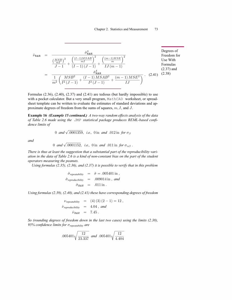
Chapter 2. Statistics and Measurement 73
Degrees ofFreedom forUse WithFormulas(2.37) and(2.38)
�R&R =�4R&R�
MSBmI
�2J � 1 +
�(I�1)MSAB
mI
�2(I � 1) (J � 1) +
�(m�1)MSE
m
�2IJ (m� 1)
=�4R&R
1
m2
�MSB2
I2 (J � 1) +(I � 1)MSAB2I2 (J � 1) +
(m� 1)MSE2IJ
� . (2.41)
Formulas (2.36), (2.40), (2.37) and (2.41) are tedious (but hardly impossible) to usewith a pocket calculator. But a very small program, MathCAD worksheet, or spread-sheet template can be written to evaluate the estimates of standard deviations and ap-proximate degrees of freedom from the sums of squares,m; I; and J .
Example 16 (Example 15 continued.) A two-way random effects analysis of the dataof Table 2.6 made using the JMP statistical package produces REML-based con�-dence limits of
0 andp:0001359; i.e., 0 in and :012 in for ��
and0 and
p:0001152; i.e., 0 in and :011 in for ��� :
There is thus at least the suggestion that a substantial part of the reproducibility vari-ation in the data of Table 2.6 is a kind of non-constant bias on the part of the studentoperators measuring the peanuts.Using formulas (2.35), (2.36), and (2.37) it is possible to verify that in this problem
�repeatability = � = :005401 in ;
�reproducibility = :009014 in ; and�R&R = :011 in :
Using formulas (2.39), (2.40), and (2.41) these have corresponding degrees of freedom
�repeatability = (4) (3) (2� 1) = 12 ;�reproducibility = 4:04 ; and
�R&R = 7:45 :
So (rounding degrees of freedom down in the last two cases) using the limits (2.38),95% con�dence limits for �repeatability are
:005401
r12
23:337and :005401
r12
4:404

74 Chapter 2. Statistics and Measurement
i.e.:0039 in and :0089 in ;
approximate 95% con�dence limits for �reproducibility are
:009014
r4
11:143and :009014
r4
:484
i.e.:0054 in and :0259 in ;
and approximate 95% con�dence limits for �R&R are
:011
r7
16:013and :011
r7
1:690
i.e.:0073 in and :0224 in :
These intervals show that none of these standard deviations are terribly well-determined(degrees of freedom are small and intervals are wide). If better information is needed,more data would have to be collected. But there is at least some indication that�repeatability and �reproducibility are roughly of the same order of magnitude. The caliperused to make the measurements was a fairly crude one, and there were detectable dif-ferences in the way the student operators used that caliper.Suppose, for sake of example, that engineering requirements on these Styrofoam
peanuts were that they be of size :50 in� :05 in. In such a context, the gauge capabilityratio (2.29) could be estimated to be between
6 (:0073)
:65� :55 = :44 and6 (:0224)
:65� :55 = 1:34
These values are not small. (See again the discussion on page 66.) This measurement"system" is not really adequate to check conformance to even these crude �:05 inproduct requirements.
Some observations regarding the planning of a gauge R&R study are in order atthis point. The precisions with which one can estimate �; �reproducibility; and �R&Robviously depend upon I; J , and m: Roughly speaking, precision of estimation of� is governed by the product (m � 1)IJ; so increasing any of the "dimensions" ofthe data array will improve estimation of repeatability. However, it is primarily J thatgoverns the precision with which �reproducibility and �R&R can be estimated. Onlyby increasing the number of operators in a gauge R&R study can one substantiallyimprove the estimation of reproducibility variation.While this fact about the estimation of reproducibility is perfectly plausible, its im-
plications are not always fully appreciated (or at least not kept clearly in mind) byquality assurance practitioners. For example, many standard gauge R&R data collec-tion forms allow for at most J = 3 operators. But three is a very small sample size

Chapter 2. Statistics and Measurement 75
when it comes to estimating a variance or standard deviation. So although the data inTable 2.1 are perhaps more or less typical of many R&R data sets, the small (J = 3)number of operators evident there should not be thought of as in any way ideal. Toget a really good handle on the size of reproducibility variation, many more operatorswould be needed.
Section 2.4 Exercises1. Consider again the situation of problem 3 of the Section 2.3 exercises and thedata from the Fiber Angle case used there. (Operator 1 measured �ber anglefor 3 different specimens 4 times each.) Recast that scenario into the two-wayframework of this section.
(a) Give the values of I; J; andm.
(b) Find a range-based estimate of �device .
(c) Find a range-based estimate of �x.
2. Based only on the data of problem 3 of the Section 2.3 exercises, can �reproducibilitybe estimated? Why or why not?
3. Consider again the situation of problems 2 and 1 of the Section 2.3 exercises andthe data from the Fiber Angle case used there. (Fiber angle for specimen 1 wasmeasured 4 times by each of operators 1, 2, and 3.) Recast that scenario into thetwo-way framework of this section.
(a) Give the values of I; J; andm.
(b) Find a range-based estimate of �repeatability .
(c) Find a range-based estimate of �reproducibility.
(d) Based only on the data considered here, can �x be estimated? Why or whynot?
4. Washer Assembly. Sudam, Heimer and Mueller studied a clothes washer baseassembly. Two operators measured the distance from one edge of a washer baseassembly to an attachment. For a single base assembly, the same distance wasmeasured four times by each operator. This was repeated on 3 different baseassemblies. The target distance was 13:320 with an upper speci�cation of U =13:42 and a lower speci�cation of of L = 13:22. A standard gauge R & R studywas conducted and data like those below were obtained. (Units are 10�1 in.)
Operator 1 Operator 2Part 1 13:285; 13:284; 13:283; 13:282 13:284; 13:288; 13:287; 13:283Part 2 13:298; 13:293; 13:291; 13:291 13:297; 13:292; 13:292; 13:293Part 3 13:357; 13:356; 13:354; 13:356 13:355; 13:354; 13:352; 13:357

76 Chapter 2. Statistics and Measurement
(a) What were the values of I; J; andm in this study?(b) Based on the ANOVA table for the data given below, �nd the estimates for
�repeatability;�reproducibility; and �R&R.(c) Give 95% con�dence limits for �repeatability , �reproducibility and �R&R.(d) Find 95% con�dence limits for the GCR. (Hint: Use the last of your an-
swers to (c).)
ANOVA TableSource SS df MSPart :0236793 2 :0118396Operator :0000007 1 :0000007Part�Operator :0000106 2 :0000053Error :0000895 18 :0000050Total :0237800 23
2.5 Simple Linear Regression and Calibration StudiesCalibration is an essential activity in the quali�cation and maintenance of measurementdevices. In a calibration study, one uses a measurement device to produce measure-ments on "standard" specimens with (relatively well-) "known" values of measurands,and sees how the measurements compare to the known values. If there are systematicdiscrepancies between what is known to be true and what the device reads, a conver-sion scheme is created to (in future use of the device) adjust what is read to somethingthat is hopefully closer to the (future) truth. A slight extension of "regression" analysis(curve �tting) as presented in an elementary statistics course is the relevant statisticalmethodology in making this conversion. (See, for example, Section 9.1 of Vardemanand Jobe's Basic Engineering Data Collection and Analysis.) This section discussesexactly how regression analysis is used in calibration.Calibration studies employ true/gold-standard-measurement values of measurands
x and "local" measurements y. (Strictly speaking, y need not even be in the sameunits as x.) Regression analysis can provide both "point conversions" and measures ofuncertainty (the latter through inversion of "prediction limits"). The simplest version ofthis is where observed measurements are approximately linearly related to measurands,i.e.
y � �0 + �1x
This is "linear calibration." The standard statistical model for such a circumstance isSimple LinearRegressionModel
y = �0 + �1x+ � (2.42)
for a normal error � with mean 0 and standard deviation �. (� describes how muchy's vary for a �xed x, and in the present context typically amounts to a repeatabilitystandard deviation.) This model can be pictured as in Figure 2.17.

Chapter 2. Statistics and Measurement 77
FIGURE 2.17. A schematic of the usual simple linear regression model (2.42)
For n data pairs (xi; yi), simple linear regression methodology allows one to makecon�dence intervals and tests associated with the model, and prediction limits for anew measurement ynew associated with a new measurand, xnew. These are of the form
PredictionLimitsfor ynew in SLR(b0 + b1xnew)�tsLF
s1 +
1
n+(xnew � �x)2Pi(xi � �x)2
(2.43)
where the least squares line is y = b0 + b1x and sLF (a "line-�tting" sample standarddeviation) is an estimate of � derived from the �t of the line to the data. Any goodstatistical package will compute and plot these limits as functions of xnew along with aleast squares line through the data set.
Example 17 Measuring Cr6+ Concentration With a UV-vis Spectrophotometer. Thedata below were taken from a Web page of the School of Chemistry at the Universityof Witwatersrand developed and maintained by Dr. Dan Billing. They are measuredabsorbance values, y, for n = 6 solutions with "known" Cr6+ concentrations, x (inmg= l), from an analytical lab.
x 0 1 2 4 6 8y :002 :078 :163 :297 :464 :600
Figure 2.18 on page 78 is a plot of these data, the corresponding least squares line,and the prediction limits (2.43).
What is here of most interest about simple linear regression technology is what it saysabout calibration and measurement in general. Some applications of inference methodsbased on the model (2.42) to metrology are the following.

78 Chapter 2. Statistics and Measurement
0 2 4 6 8
0.0
0.2
0.4
0.6
FIGURE 2.18. Scatterplot of the Cr6+ Concentration calibration data, least squares line, andprediction limits for ynew
1. From a simple linear regression output,
sLF =pMSE =
vuut 1
n� 2
nXi=1
(yi � yi)2 = "root mean square error" (2.44)
is an estimated repeatability standard deviation. One may make con�dence in-tervals for � = �repeatability based on the estimate (2.44) using � = n� 2 degreesof freedom and limits
Con�denceLimits for � inModel (2.42)
sLF
sn� 2�2upper
and sLF
sn� 2�2lower
: (2.45)
2. The least squares equation y = b0 + b1x can be solved for x, giving
CoversionFormula fora FutureMeasurment,ynew
xnew =ynew � b0b1
(2.46)
as a way of estimating a new "gold-standard" value (a new measurand, xnew)from a measured local value, ynew.

Chapter 2. Statistics and Measurement 79
3. One can take the prediction limits (2.43) for ynew and "turn them around" toget con�dence limits for the xnew corresponding to a measured local ynew. Thisprovides a defensible way to set "error bounds" on what ynew indicates aboutxnew.
4. In cases (unlike Example 17) where y and x are in the same units, con�dencelimits for the slope �1 of the simple linear regression model
Con�denceLimits for �1 inModel (2.42)
b1 � tsLFqP(xi � �x)2
(2.47)
provide a way of investigating the constancy of bias (linearity of the measure-ment device in the sense introduced on page 36). That is, when x and y are inthe same units, �1 = 1:0 is the case of constant bias. If con�dence limits for �1fail to include 1:0, there is clear evidence of device nonlinearity.
Example 18 (Example 17 continued.) Use of the JMP statistical package with thedata of Example 17 produces
y = :0048702 + :0749895x with sLF = :007855 :
We might expect a local (y) repeatability standard deviation of around :008 (in the yabsorbance units). In fact, 95% con�dence limits for � can be made (using n� 2 = 4degrees of freedom and formula (2.45)) as
:007855
r4
11:143and :007855
r4
:484;
i.e.:0047 and :0226 :
Making use of the slope and intercept of the least squares line, a conversion formulafor going from ynew to xnew is (as in display (2.46))
xnew =ynew � :0048702:0749895
;
So, for example, a future measured absorbance of ynew = :20 suggests a concentrationof
xnew =:20� :0048702:0749895
= 2:60mg= l :
Finally, Figure 2.19 on page 80 is a modi�cation of Figure 2.18 that illustrates howthe plotted prediction limits (2.43) provide both 95% predictions for a new measure-ment on a �xed/known measurand and 95% con�dence limits on a new measurand,

80 Chapter 2. Statistics and Measurement
FIGURE 2.19. Con�dence limits for xnew based on an observed ynew (and prediction limits(2.43))
having observed a particular measurement. Reading from the �gure, one is "95% sure"that a future observed absorbance of :20 comes from a concentration between
2:28mg= l and 2:903mg= l :
Example 19 A Check on Device "Linearity." A calibration data set due to John Man-del compared n = 14 measured values y for a single laboratory to corresponding con-sensus values x for the same specimens derived from multiple labs. (The units are notavailable, but were the same for x and y values.) A simple linear regression analysisof the data pairs produced
b1 = :882 andsLFqP(xi � �x)2
= :012
so that (using the upper 2.5% point of the t12 distribution, 2:179, and formula (2.47))95% con�dence limits for �1 are
:882� 2:179 (:012)
or:882� :026 :

Chapter 2. Statistics and Measurement 81
A 95% con�dence interval for �1 clearly does not include 1:0. So bias for the singlelaboratory was not constant. (The measurement "device" was not linear in the sensediscussed on page 36.)
Section 2.5 Exercises
1. n = 14 polymer specimens of known weights, x, were weighed and the mea-sured weights, y, recorded. The following table contains the data. (All units areg's:)
x 1 1 3 3 5 5 7y 1:10 :95 2:98 3:01 5:02 4:99 6:97
x 7 10 10 12 12 14 14y 7:10 10:03 9:99 12:00 11:98 14:10 14:00
(a) Find the least squares line y = b0 + b1x for these data.
(b) Find the estimated repeatability standard deviation corresponding to yourregression analysis.
(c) Find 95% con�dence limits for the y repeatability standard deviation basedon your answer to (b).
2. In the context of problem 1, suppose a new specimen is measured as having aweight of 6:10 g.
(a) Find the "calibrated weight," x, corresponding to this new specimen basedon your regression analysis.
(b) Find 95% con�dence limits for the slope of the relationship between mea-sured and actual weight (�1). Does the device used to produce the y mea-surements have constant bias (is it "linear")? Why or why not?
3. Based on your regression analysis in problem 1, �nd 95% prediction limits forthe next measured weight for a new specimen with standard known weight of8 g.
4. Would it be wise to use the above regression analyses to adjust a measured spec-imen weight of ynew = :2 g? Why or why not?

82 Chapter 2. Statistics and Measurement
2.6 Measurement Precision and the Ability to Detect aChange or Difference
Estimating the repeatability and reproducibility of a gauge or measurement systemamounts to �nding a sensible standard deviation ("sigma") to associate with it. Whereonly one operator is involved, the repeatability measure, �, is appropriate. Where mul-tiple operators are going to be used, the measure �R&R de�ned in display (2.27) ismore germane. After an appropriate sigma has been identi�ed, it can form the basis ofjudgments concerning the adequacy of the gauge or system for speci�c purposes. Forexample, looking at measures like the gauge capability ratio (2.29) is a way of judging(based on an appropriate sigma) the adequacy of a gauge for the purpose of check-ing conformance to a set of engineering speci�cations. In this section, we consider theslightly different matter of the adequacy of a gauge or measurement system for thepurpose of detecting a change or difference.The problem of determining whether "something has changed"/"there is a differ-
ence" is fundamental to engineering and technology. For example, in the context ofprocess monitoring, engineers need to know whether process parameters (e.g., themean widget diameter being produced by a particular lathe) are at standard valuesor have changed. And, in evaluating whether two machines are producing similar out-put, one needs to assess whether product characteristics from the two machines are thesame or are consistently different. And, for example, when using hazardous materialsin manufacturing, engineers need to compare chemical analyses for current environ-mental samples to analyses for "blank" samples, looking for evidence that importantquantities of toxic materials have escaped a production process and thus increased theirambient level from some "background" level.For the remainder of this section, let �measurement stand for an appropriate standard
deviation for describing the precision of some measurement system. (Depending uponthe context this could be � or �R&R from a gauge R&R study.) We will investigatethe impact of �measurement on one's ability to detect change or difference throughconsideration of the distribution of the statistic
ynew � yold ; (2.48)
where ynew is the sample mean of nnew independent measurements taken on a particu-lar "new" object and yold is the sample mean of nold independent measurements takenon a particular "old" object. This is much like the context of Section 2.2.2, and Fig-ure 2.20 (which is a slight modi�cation of Figure 2.12) illustrates the situation underconsideration. The related issue issue of how to think about situations where particularobjects being measured are themselves of interest only to the extent that they represent"new" and "old" conditions that produced them will be considered brie�y at the end ofthis section.This discussion will allow the possibility that the information on the "old" object is

Chapter 2. Statistics and Measurement 83
FIGURE 2.20. nold measurements on an "old" measurand and nnew measurements on a "new"measurand made with a single system with (constant) bias � and measurement standard deviation�measurement
strong enough that nold can be thought of as being essentially in�nite, and thus yoldessentially equal to the (long-run) mean of old observations, xold + �. If xnew + �is the long-run mean (expected value) of the new observations and the new and oldmeasurements are independent, the random variable in display (2.48) has mean
Mean for theRandomVariableynew � yold
E(ynew � yold) = (xnew + �)� (xold + �) = xnew � xold ; (2.49)
and variance
Variance for theRandomVariableynew � yold
Var(ynew � yold) = �2measurement�
1
nnew+
1
nold
�: (2.50)
When the information on the old object is strong enough to consider nold to be essen-tially in�nite, expression (2.50) reduces to
Var(ynew � yold) = �2measurement�
1
nnew
�: (2.51)
In the event that it is sensible to think of ynew � yold as normally distributed (eitherbecause repeat measurements are themselves approximately normally distributed orbecause both nnew and nold are large) one then has the picture of the distribution ofynew � yold given in Figure 2.21 on page 84. If xnew = xold, then the normal curve inthe �gure is centered at 0. If xnew 6= xold the normal curve in the �gure is centered atthe nonzero difference between the new and old measurands.
Example 20 Chemical Analysis for Benzene. An appropriate standard deviation forcharacterizing an industrial laboratory's precision in a particular analysis for the ben-zene content of samples of a particular type is �measurement = :03� g= l. Suppose thatin order to determine whether the amount of benzene in a particular environmentalsample exceeds that in a particular similar "blank" sample (supposedly containing

84 Chapter 2. Statistics and Measurement
FIGURE 2.21. The distribution of ynew � yold
only background levels of the substance), the environmental sample will be analyzednnew = 1 time and its measured content compared to the mean measured content fromnold = 5 analyses of a single blank sample. Then from equations (2.49) and (2.50) therandom variable ynew � yold has mean
E(ynew � yold) = xnew � xold ;
and standard deviation
pVar(ynew � yold) = �measurement
r1
1+1
5= :03
r6
5= :033� g= l :
Figure 2.22 shows a corresponding probability distribution for the difference ynew �yold assuming that repeat measurements of a given sample are normally distributed.Note, by the way, that if the information on the blank sample was essentially perfect
and equation (2.51) was relevant, the standard deviation associated with ynew � �oldwould be :030�g=l, not much smaller than the :033�g=l value found here.
FIGURE 2.22. Distribution of ynew � yold in the benzene analysis example

Chapter 2. Statistics and Measurement 85
The picture of ynew � yold given in equations (2.49) and (2.50) and Figure 2.21forms the basis for several common ways of evaluating the adequacy of a measurementtechnique to characterize a change or difference. One simple-minded rule of thumboften employed by analytical chemists is that a difference xnew � xold needs to be onthe order of 10 times the standard deviation of ynew � yold before it can be adequatelycharacterized by a measurement process with standard deviation �measurement usingsample sizes nnew and nold. For example, in the benzene analyses of Example 20, withsample sizes nnew = 1 and nold = 5, this rule of thumb says that only increases in realbenzene content on the order of at least
10� :033 = :33� g= l
can be reliably characterized. This somewhat ad hoc (but nevertheless popular) guide-line amounts to a requirement that one's "signal-to-noise ratio" for determination of adifference (ratio of mean to standard deviation) be at least 10 before being comfortablewith the resulting precision.A second approach to using the picture of ynew � yold given in equations (2.49)
and (2.50) and Figure 2.21 to describe one's ability to detect a difference betweenmeasurands involves some ideas from hypothesis testing. In interpreting an observedvalue of ynew � yold, one might require that it be of a certain minimum magnitudebefore declaring that there is clearly a difference between new and old objects. For thesake of concreteness, suppose for the rest of this section that one is concerned aboutdetecting an increase in response. That is, suppose one is interested in detecting thepossibility that xnew � xold > 0. It then makes sense to set some critical limit, Lc,and to only declare that there has been a change (that there is a difference) if
ynew � yold > Lc : (2.52)
If one wishes to limit the probability of a "false positive" (i.e., a type I error) Lc shouldbe large enough that the eventuality (2.52) occurs rarely when in fact xnew = xold. Forexample, if one may assume that ynew � yold is essentially normally distributed, it ispossible to use the fact that when xnew = xold the variable
ynew � yold�measurement
q1
nnew+ 1
nold
is standard normal, to set a value for Lc. From a normal table, one may pick a numberz1 so that for standard normal Z, P [Z > z1] = �, for � a small number of one'schoosing. Then setting

86 Chapter 2. Statistics and Measurement
Critical Valuefor Normalynew � yoldif an Increase inResponse Isto Be Detected Lc = z1�measurement
r1
nnew+
1
nold; (2.53)
the probability of a false positive is no more than �.Once one has established a critical value Lc (using equation (2.53) or otherwise)
it is then reasonable to ask what is the probability of detecting a change of a givensize, or equivalently what size change can be reliably detected. Again, assuming thatynew�yold is essentially normally distributed as in Figure 2.21, it is possible to answerthis question. That is, using the normal model, with
z-score for theCritical ValueLc
z2 =Lc � (xnew � xold)
�measurement
q1
nnew+ 1
nold
; (2.54)
the probability (depending upon xnew�xold) of declaring that there has been a change(that there is a difference) is
Probability ofDeclaring ThatResponse HasIncreased (forNormalynew � yold)
= P [Z > z2] ; (2.55)
(for Z again standard normal). Or by rewriting equation (2.54), for z2 chosen so that in display (2.55) is large, one can solve for the size of change in measurand requiredto produce a large (at least ) probability of detection, namely
Change inMeasurandwith Probability ofDetection (forNormalynew � yold)
xnew � xold = Lc � z2�measurementr
1
nnew+
1
nold: (2.56)
Notice that in display (2.56) z2 is typically negative so that this difference in mea-surands xnew � xold is then typically larger than Lc.In analytical chemistry, the value of xnew � xold required to produce a large proba-
bility of detecting an increase in measurand is given a special name.

Chapter 2. Statistics and Measurement 87
De�nition 21 For a given standard deviation of measurement �measurement, samplesizes nnew and nold, critical value Lc and desired (large) probability , the lower limitof detection, Ld, of a measurement protocol is the smallest difference in measurandsxnew � xold producing
P [ynew � yold > Lc] � :
When ynew � yold is normal and z2 is chosen according to display (2.55), equation(2.56) implies that
Lower Limit ofDetection (forNormalynew � yold)Ld = Lc � z2�measurement
r1
nnew+
1
nold: (2.57)
(where again, z2 is typically negative so that this Ld is then typically larger than Lc).And although there is no requirement that Lc be set according to equation (2.53), whenthis is used to control the chance of a false positive, equations (2.53) and (2.57) com-bine to produce
Lower Limit ofDetection ifEquation (2.53)is Used to Setthe CriticalValue andEquation (2.55)is Used
Ld = (z1 � z2)�measurementr
1
nnew+
1
nold(2.58)
Example 22 (Example 20 continued.) Consider again the benzene analysis example.Suppose that it is desirable to limit the probability of producing a "false positive"(a declaration that the environmental sample contains more benzene than the blanksample when in fact there is no real difference in the two) to no more than � = :10.Consulting a standard normal table, for Z standard normal, P [Z > 1:282] = :10. So,using equation (2.53), an appropriate critical value is
Lc = 1:282(:030)
r1
1+1
5= :042:
Should one wish to evaluate the probability of detecting an increase in real benzenecontent of size xnew � xold = :02� g= l using this critical value, equations (2.54) and(2.55) show that with
z2 =:042� :02
:030q
11 +
15
= :67;
the probability is only about
P [Z > z2] = P [Z > :67] = :2514:

88 Chapter 2. Statistics and Measurement
There is a substantial (75%) chance of failing to identify a .02� g= l increase in benzenecontent beyond that resident in the blank sample. This unpleasant fact motivates thequestion "How big does the increase in benzene concentration need to be in orderto have a large (say 95%) chance of seeing it above the measurement noise?" Sinceconsultation of the standard normal table shows that
P [Z > �1:645] = :95;
equations (2.55) and (2.57) imply that for = :95
Ld = xnew � xold = :042� (�1:645)(:030)r1
1+1
5= :096� g= l
is (in the language of De�nition 21) the lower limit of detection in this situation. A realincrease in benzene content must be of at least this size for there to be a large (95%)chance of "seeing" it through the measurement noise.
The particular example used in the foregoing discussion of the implications of equa-tions (2.49) and (2.50) and Figure 2.21 is from analytical chemistry. But the basicmethod illustrated is perfectly general and could, for example, be equally well appliedto the consideration of the implications of measurement precision for one's ability todetect a difference in diameters of two particular parts turned on a lathe.It is, however, an extremely important distinction that the discussion thus far in this
section has been phrased in terms of detecting a difference between two particular ob-jects and not between processes or populations standing behind those objects. Example20 concerns comparison of a particular environmental sample and a particular blanksample. It does not directly address the issue of how the population of environmentalsamples from a site of interest compares to a population of blanks. Similarly, in a man-ufacturing context, comparisons based on the foregoing material would concern twoparticular measured parts, not the process conditions operative when those parts weremade. The point here is that only measurement variation has been taken into account,and not object-to-object variation for processes or populations the measured objectsmight represent. (And unless there is no "within-population" or "process" variation,detection of a difference between an old and a new object is not the same as detectionof a difference between old and new population or process means.)The problem of comparing two processes or populations while admitting the reality
of measurement noise was �rst raised in Section 2.2.2. Figure 2.23 is a slight modi�ca-tion of Figure 2.13 from that section and represents the scenario under consideration.In this second context, the difference in sample means (2.48) has mean
E(ynew � yold) = (�xnew + �)� (�xold + �) = �xnew � �xold ;
the difference in process or condition mean measurands. The variance of the difference

Chapter 2. Statistics and Measurement 89
FIGURE 2.23. nold measurements on an "old" process and nnew measurements on a "new"process made with a single system with (constant) bias � and measurement standard deviation�measurement
is
Var(ynew � yold) =�2xnew + �
2measurement
nnew+�2xold + �
2measurement
nold
= �2measurement
�1
nnew+
1
nold
�+�2xnewnnew
+�2xoldnold
and (of course) item-to-item/measurand-to-measurand variability is re�ected in ynew�yold. In the event that the "old" and "new" processes have comparable values of �x,the formulas and language in this section can be reinterpreted to allow applicationto the problem of detecting changes in a process or population mean, by replacing�measurement with q
�2x + �2measurement
Otherwise, a separate development of formulas is required. For example, if in the con-text of Example 20, blank samples are more homogeneous than are �eld samples froma particular site, an analysis parallel to that in this section but based on the two differentvalues for �x will be needed for application to the problem of comparing a site meanbenzene level to a blank mean level.
Section 2.6 Exercises1. An analyst can tolerate only a .01 (1%) chance of falsely concluding that a mea-surand associated with a �eld sample exceeds that for a blank (should thoseactually be the same).

90 Chapter 2. Statistics and Measurement
(a) In the context of the discussion of this section, what value of z1 is thenappropriate?
(b) The analyst was also interested in identifying the smallest positive differ-ence in measurands (x�eld � xblank) for which there is probability of only.05 of incorrectly concluding the difference is zero or negative. What valueshould this person use for z2?
(c) Using your values for z1 and z2 from (a) and (b) above and equation (2.58),what is the lower limit of detection for this scenario if only single measure-ments are made on both the �eld sample and the blank? (Your answer willbe a multiple of �measurement.)
2. Dimethyl Phenanthrene (DMP4) Atmospheric Blank. Currie, et al. presentedthe paper "Impact of the Chemical and Isotopic Blank on the Interpretation ofEnvironmental Radiocarbon Results" at the International Radiocarbon Confer-ence in Glasgow, Scotland, August 1994. Their presentation included discussionof six measurements of the DMP4 content of an atmospheric �eld �lter blank.(DMP4 is a product of softwood pyrolysis.) The six responses in nanograms(10�9 g) were
8:25; 7:30; 7:27; 6:54; 6:75 and 7:32:
Suppose here that one analyst measured the DMP4 �eld �lter blank all six timeswith the same instrument.
(a) Find the sample standard deviation of these values. In terms of the gaugeR&R material of Section 2.4, what does this sample standard deviationestimate? In parts (b), (c) and (d) below, use this estimate as if it were thetrue value of �measurement.
(b) Find a critical limit, Lc, if the probability of a false positive detection is tobe 10% and both a �eld sample and a (new) blank are to be measured once.
(c) Find a lower limit of detection where the probability of a false positivedetection is 10% and the probability of a false negative is to be 5% for adifference in measurands at the lower limit of detection. (Suppose as inpart (b) that both a �eld sample and a new blank are to be measured once.)
(d) Continuing under the assumption that a single individual made all six mea-surements, what must be true about the measurement method if the samplestandard deviation in (a) is reasonably thought of as estimate of "�measurement"?(Consider the ideas of Section 2.4.)

Chapter 2. Statistics and Measurement 91
2.7 R&R Considerations for Go/No-Go InspectionIdeally, observation of a process results in quantitative measurements. But there aresome contexts in which all that is determined is whether an item or process condi-tion is of one of two types, that we will for the present call "conforming" and "non-conforming." It is, for example, common to check the conformance of machined metalparts to some engineering requirements via the use of a "go/no-go gauge." (A part isconforming if a critical dimension �ts into the larger of two check �xtures and does not�t into the smaller of the two.) And it is common to task human beings with makingvisual inspections of manufactured items and producing a "OK/Not-OK" call on each.Engineers are sometimes then called upon to apply the qualitative "repeatability"
and "reproducibility" concepts of metrology to such Go/No-Go or "0/1" contexts. Onewants to separate some measure of overall inconsistency in 0/1 "calls" on items intopieces that can be mentally charged to inherent inconsistency in the equipment ormethod, and the remainder that can be charged to differences between how operatorsuse it. Exactly how to do this is presently not well-established. The best available statis-tical methodology for this kind of problem is more complicated than can be presentedhere (involving so-called "generalized linear models" and random effects in these).What we can present is a rational way of making point estimates of what might betermed repeatability and reproducibility components of variation in 0/1 calls. (Theseare based on reasoning similar to that employed in Section 2.4.2 to �nd correct range-based estimates in usual measurement R&R contexts.) We then remind the reader ofelementary methods of estimating differences in population proportions and point outtheir relevance in the present situation.
2.7.1 Some Simple Probability ModelingTo begin, think of coding a "non-conforming" call as "1" and a "conforming" call as"0," and having J operators each makem calls on a �xed part. Suppose that J operatorshave individual probabilities p1; p2; : : : ; pJ of calling the part "non-conforming" onany single viewing, and that acrossm viewings
Xj = the number of non-conforming calls among them made by operator j
is Binomial (m; pj). We'll assume that the pj are random draws from some populationwith mean � and variance v.The quantity
pj (1� pj)
is a kind of "per call variance" associated with the declarations of operator j, andmight serve as a kind of repeatability variance for that operator. (Given the value ofpj , elementary probability theory says that the variance of Xj is mpj (1� pj).) Thebiggest problem here is that unlike what is true in the usual case of gauge R&R for

92 Chapter 2. Statistics and Measurement
measurements, this variance is not constant across operators. But its expected value,namely
E (pj (1� pj)) = � � Ep2j= � �
�v + �2
�= � (1� �)� v
can be used as a sensible measure of variability in conforming/non-conforming clas-si�cations chargeable to repeatability sources. The variance v serves as a measure ofreproducibility variance. This ultimately points to
� (1� �)
as the "total R&R variance" here. That is, we make de�nitions for 0/1 contextsR&R Variancefor One Part ina 0/1 Context
�2R&R = � (1� �) (2.59)
RepeatabilityVariance forOne Part in a0/1 Context
�2repeatability = � (1� �)� v (2.60)and
ReproducibilityVariance forOne Part in a0/1 Context
�2reproducibility = v (2.61)
2.7.2 Simple R&R Point Estimates for 0/1 ContextsStill thinking of a single �xed part, let
pj =the number of "non-conforming" calls made by operator j
m=Xjm
and de�ne the (sample) average and (sample) variance of these,
�p =1
J
JXj=1
pj and s2p =1
J � 1
JXj=1
�pj � �p
�2:
It is possible to argue thatE �p = �
and that
Es2p = Varpj
= Varpj + Epj (1� pj)
m
=m� 1m
v +� (1� �)
m;
so thatv =
m
m� 1Es2p �
� (1� �)m� 1 :

Chapter 2. Statistics and Measurement 93
This line of reasoning suggests the simple estimators (still based on a single part)Estimator ofR&R Variancefor a SinglePart in a 0/1Context�2R&R =
�p�1� �p
�(2.62)
and
�2reproducibility = max
�0;
1
m� 1�ms2p � �p
�1� �p
���(2.63)
On rare occasions, s2p will exceed �p�1� �p
�, leading to a value of �2reproducibility in dis-
play (2.63) larger than �2R&R speci�ed in display (2.62). In those cases we will reduce�2reproducibility to �
2R&R =
�p�1� �p
�and thus produce a �nal version of the estimator
(2.63)Estimator ofReproducibilityVariance for aSingle Part in a0/1 Context�2reproducibility = min
��2R&R;max
�0;
1
m� 1�ms2p � �p
�1� �p
����. (2.64)
Then from displays (2.62) and (2.64) an obvious estimator of the repeatability varianceis
Estimator ofRepeatabilityVariance for aSingle Part in a0/1 Context�2repeatability = �
2R&R � �2reproducibility (2.65)
Again, the estimators (2.62), (2.64), and (2.65) are based on a single part. Exactlywhat to do based on multiple parts (say I of them) is not completely obvious. But inorder to produce a simple methodology, we will simply average estimates made onepart at a time across multiple parts, presuming that parts in hand are sensibly thoughtof as a random sample of parts to be checked, and that this averaging is a reasonableway to combine information across parts.In order for any of this to have a chance of working, m will need to be fairly large.
The usual gauge R&R "m = 2 or 3" just isn't going to produce informative results inthe present context. And in order for this to work in practice (so that an operator isn'tjust repeatedly looking at the same few parts over and over and remembering how heor she has called them in the past) a large value of I may also be needed.

94 Chapter 2. Statistics and Measurement
TABLE 2.7. Hypothetical Results of Visual Inspection of 5 Parts by 3 OperatorsOperator 1 Operator 2 Operator 3 �p �p
�1� �p
�s2p
Part 1 :2 :4 :2 :2667 :1956 :0133Part 2 :6 :6 :7 :6333 :2322 :0033Part 3 1:0 :8 :7 :8333 :1389 :0233Part 4 :1 :1 :1 :1 :0900 0Part 5 :1 :3 :3 :2333 :1789 :0133
TABLE 2.8. R&R Cacluations for the Hypothetical Visual Inspection Data�2R&R =
�p�1� �p
��2reproducibility �2repeatability
Part 1 :1956 0 :1956Part 2 :2322 0 :2322Part 3 :1389 :0105 :1284Part 4 :0900 0 :0900Part 5 :1789 0 :1789Average :1671 :0021 :1650
Example 23 A Simple Numerical Example. For purposes of illustrating the formulasof this section, we will use a small numerical example due to Prof. Max Morris. Sup-pose that I = 5 parts are inspected by J = 3 operators, m = 10 times apiece, andthat in Table 2.7 are sample fractions of "non-conforming" calls made by the operatorsand a few summary statistics.The entries in the next to last column of Table 2.7 are �2R&R values for the 5 parts.
Estimates of �2reproducibility are, for example, computed as for Part 1
�2reproducibility = max
�0;
1
10� 1 (10 (:0133)�:1956)�
= 0
leaving estimates of �2repeatability computed as for Part 1
�2repeatability = :1956� 0= :1956
The whole set of estimates and their averages are collected in Table 2.8.Then, for example, a fraction of only
:0021
:1671= 1:3%
of the inconsistency in conforming/non-conforming calls seen in the original dataseems to be attributable to clear differences in how the operators judge the parts (dif-ferences in the binomial "success probabilities" pj). Rather, the bulk of the varianceseems to be attributable to unavoidable binomial variation. The p's are not closeenough to either 0 or 1 to make the calls tend to be consistent. So the variation seenin the p's in a given row is not clear evidence of large operator differences.

Chapter 2. Statistics and Measurement 95
Of course, we need to remember that the computations above are on the variance(and not standard deviation) scale. On the (more natural) standard deviation scale,reproducibility variation p
:0021 = :05
and repeatability variation p:1650 = :41
are not quite so strikingly dissimilar.
2.7.3 Application of Inference Methods for the Difference in TwoBinomial "p's"
The question of whether call rates for two operators on the same part are really de-tectably different brings up the elementary statistics topic of estimating the differencein two binomial parameters, say p1 and p2: A common elementary large sample ap-proximate con�dence interval for p1 � p2 has endpoints
p1 � p2 � z
sp1 (1� p1)
n1+p2 (1� p2)
n2.
But, as it turns out, this formula can fail badly if either p is extreme or either n is small.So we will use a slight modi�cation that is more reliable, namely
Con�denceLimts forp1 � p2
p1 � p2 � z
s~p1 (1� ~p1)
n1+~p2 (1� ~p2)
n2(2.66)
whereValues to Usein Formula(2.66)
~pi =nipi + 2
ni + 4(2.67)
That is, under the square root of the usual formula one essentially replaces the p valueswith ~p values derived by adding 2 "successes" in 4 "additional trials" to the countsused to make up the p values. (This has the effect of making the standard large sampleinterval a bit wider and correcting the problem that for small sample sizes and extremevalues of p it can fail to hold its nominal con�dence level.)

96 Chapter 2. Statistics and Measurement
Example 24 (Example 23 continued.) Consider again Part 1 from Example 23, andin particular consider the question of whether Operator 1 and Operator 2 have clearlydifferent probabilities of calling that part non-conforming on a single call. With p1 =:2 and p2 = :4, formula (2.67) says that
~p1 =2 + 2
10 + 4= :2857 and ~p2 =
4 + 2
10 + 4= :4286
so that using formula (2.66) approximate 95% con�dence limits for the difference p1�p2 are
:2� :4� 1:96r:2857 (1� :2857)
10+:4286 (1� :4286)
10
i.e.�:2� :49
These limits cover 0 and there thus is no clear evidence in the p1 = :2 and p2 = :4values (from the relatively small samples of sizesm = 10) that Operators 1 and 2 havedifferent probabilities of calling Part 1 non-conforming.
Section 2.7 Exercises1. Suppose that 10 parts are inspected by 4 operators 16 times apiece. Each inspec-tion determines whether or not the item is conforming. The counts in the tablebelow correspond to the numbers of "non-conforming" calls out of 16 inspec-tions.
Operator 1 Operator 2 Operator 3 Operator 4Part 1 10 11 11 10Part 2 11 9 12 10Part 3 8 8 9 7Part 4 15 14 14 16Part 5 12 14 11 12Part 6 15 15 16 15Part 7 14 11 14 12Part 8 16 16 15 15Part 9 13 15 14 15Part 10 16 15 16 16
(a) Using the data above, �ll in the table below:Part bp bp(1� bp) s2p12...10

Chapter 2. Statistics and Measurement 97
(b) What is the fraction of inconsistency in conforming/non-conforming callsthat can be attributed to clear differences in how the operators judged theparts (differences in the binomial "success probabilities" pj)? (Make youranswer on the variance scale.)
(c) What is the estimated reproducibility variation (on the standard deviationscale)?
(d) What is the estimated repeatability variation (on the standard deviationscale)?
(e) For part 10, give a 90% con�dence interval for the difference (operator 1minus operator 3) in probabilities of a non-conforming call. Does it appearthe operators 1 and 3 have different probabilities of a non-conforming callon any one of the parts? Why?
2.8 Chapter SummaryThis chapter has been concerned with how measurement error impacts what can belearned from empirical data. It presented some ideas from the probability modeling ofmeasurement variation, and considered how the interpretation of elementary statisticalinferences is affected by measurement error. Then a variety of more advanced statisticaltools were discussed, because of their usefulness in quantifying, partitioning, and (insome cases) removing the effects of measurement variation in quality assurance andimprovement projects.
2.9 Chapter 2 Exercises1. Does a perfectly calibrated device return measurements of a measurand that arecompletely free of error? Explain.
2. Is a standard (an item with corresponding "known" measurand) needed in bothdevice calibration and estimation of �device? If not, which requires a standard?Explain.
3. A measurement device may have a bias as large as 1 unit (in absolute value)and a device standard deviation as large as 1 unit. You measure x and observey = 10. If you believe in the simple (normal) measurement model and wantto report an interval you are "at least 99% sure" contains x, you should reportwhat limits? (Hint: Before measurement, how far do you expect y to be from xwith the indicated worst possible values of absolute bias and standard deviation?Interpret "99% sure" in "plus or minus 3 standard deviations" terms.)

98 Chapter 2. Statistics and Measurement
4. The same axel diameter is measured n1 = 25 times with device #1 and n2 =25 times with device #2, with resulting means and standard deviations y1 =2:001 in; y2 = 2:004 in; s1 = :003 in; and s2 = :004 in. The upper 2.5% pointof the F24;24 distribution is about 2:27.
(a) Give 95% con�dence limits for the difference in device biases.(b) Give 95% con�dence limits for the ratio of the two device standard devia-
tions.(c) Is there a clear difference in device biases based on your interval in (a)?
Why or why not?(d) Is there a clear difference in device standard deviations based on your in-
terval in (b)? Why or why not?
5. Two different (physically stable) production lines produce plastic pop bottles.Suppose n1 = 25 bottles from line #1 and n2 = 25 bottles from line #2 areburst-tested on a single tester, with resulting means and standard deviations y1 =201psi; y2 = 202psi; s1 = 3psi; and s2 = 4psi.
(a) Give a 95% con�dence interval for the difference between the mean burststrengths for lines #1 and #2 (line #1 minus line #2).
(b) Give a 95% con�dence interval for the ratio of burst strength standard de-viations (line #1 divided by line #2). The upper 2.5% point of the F24;24distribution is about 2.27.
(c) Is there a clear difference between mean burst strengths? Why or why not?(d) Is there a clear difference between the consistencies of burst strengths?
Why or why not?
6. Using a single tester, a single metal specimen was tested for Brinell hardness 20times with resulting sample standard deviation of hardness 10HB. Subsequently,40 different specimens cut from the same ingot of steel have sample standarddeviation of measured hardness 20HB (using the same tester).
(a) Give 95% con�dence limits for a "test variability" standard deviation.(b) Give approximate 95% con�dence limits for a specimen-to-specimen stan-
dard deviation of actual Brinell hardness.
7. An ANOVA analysis of a gauge R&R data set produced �R&R = 53 (in appropri-ate units) and b�R&R = 3. In these units, engineering speci�cations on a criticaldimension of a machined steel part are nominal � 200. Give approximate 95%con�dence limits for a GCR (gauge capability ratio) for checking conformanceto these speci�cations.
8. 95% con�dence limits for a particular gauge capability ratio are 6 to 8. Whatdoes this indicate about the usability of the gauge for checking conformance tothe speci�cations under consideration?

Chapter 2. Statistics and Measurement 99
9. Below is an analysis of variance table from a calibration study. The data werelight intensities, y (in unspeci�ed analyzer units) for specimens of known Ri-bo�avin concentration x (in �g=ml).
ANOVA TableSource SS df MSModel 10946:445 1 10946:445Error 27:155 8 3:4Total 10973:6 9
Parameter estimates for the simple linear regression model were b0 = 6:4634and b1 = 129:1768.
(a) Give a 95% con�dence interval for a repeatability standard deviation forthis analyzer.
(b) Suppose a new specimen with unknown concentration is analyzed andynew = 75 is observed. Give a single number estimate of the concentra-tion in that specimen.
10. The �nal step in the production of some glass vials is a visual inspection presentlycarried out by human inspectors. A particular single vial (marked in an "invis-ible" ink that can be seen only under ultraviolet light) known to be defective isrepeatedly run through the inspection process among a large number of newlyproduced vials. In fact, each of 5 company inspectors sees that vial 10 times in acompany study. Below are the rates at which that vial was identi�ed as defectiveby the various operators ( "1:0" means 100%.)
:6; :9; :9; 1:0; 1:0
(a) What two values of p re�ect perfect consistency of "defective/non-defective"calls made by a particular inspector?
(b) What distribution models the number of correct "defective" calls made bya particular inspector?
(c) On the scale of (estimated) variances (not standard deviations), what is thefraction of overall variation seen in the "defective/non-defective" calls forthis vial that should be attributed to operator-to-operator differences?
(d) Give 95% con�dence limits for the long run difference in proportions of"defective" calls for the �rst operator (that made 6 out of 10 "defective"calls)and the last operator (who made all "defective"calls).
11. Laser Metal Cutting. Davis, Martin and Popinga used a Ytterbium Argon gaslaser to make some cuts in 316 stainless steel. Using 95MJ/pulse and 20Hzsettings on the laser and a 15:5mm distance to the steel specimens (set at a45 � angle to the laser beam) the students made cuts in specimens using 100,500, and 1000 pulses. The measured depths of four different cuts (in machine

100 Chapter 2. Statistics and Measurement
units) at each pulse level are given below (assume the same operator made allmeasurements and that repeatability variation is negligible here).
100 Pulses 500 Pulses 1000 Pulses7:4; 8:6; 5:6; 8:0 24:2; 29:5; 26:5; 23:8 33:4; 37:5; 35:9; 34:8
(a) What is the response variable in this problem?(b) Give the sample average values for the 100, 500, and 1000 pulse levels.
Calculate the sample range for the data at each pulse level. Give estimatesof the standard deviation of cut depth for each level of pulse, �rst based onthe sample range and then using the sample standard deviation. (You willhave two estimates for each of the three population standard deviations.)
(c) Assuming variability is the same for all three pulse levels, give an estimateof the common standard deviation based on the three sample ranges.
(d) The concepts of measurement validity, precision, and accuracy are dis-cussed in Section 2.1. The analysts decided to report the average cut depthfor the different pulse levels. This averaging can be thought of in terms ofimproving which of 1) validity, 2) precision, or 3) accuracy (over the useof any single measurement)? The concept of calibration is most closelyassociated with which of the three?
12. Fiber Angle.Grunig, Hamdorf, Herman, and Potthoff studied a carpet-like prod-uct. They measured the angle at which �bers were glued to a sheet of base ma-terial. A piece of �nished product was obtained and cut into �ve sections. Eachof the four team members measured the �ber angle eight times for each section.The results of their measuring are given below (in degrees above an undisclosedreference value). A corresponding ANOVA table is also given.
(a) Say what each term in the equation yijk = � + �i + �j + ��ij + �ijkmeans in this problem (including the subscripts i, j, and k).
(b) Using ranges, estimate the repeatability and reproducibility standard devi-ations for angle measurement. Based on this analysis what aspect of themeasuring procedure seems to need the most attention? Explain.
(c) Using ANOVA-based formulas, estimate the repeatability and reproducibil-ity standard deviations for angle measurement. Is this analysis in essentialagreement with that in part (b)? Explain.
(d) Using your answer to (c), give an estimate of the standard deviation thatwould be experienced by many analysts making a single measurement onthe same angle (in the same section) assuming there is no repeatabilitycomponent to the overall variation.
(e) Speci�cations on the �ber angle are nominal � 5 �. Estimate the gaugecapability ratio using �rst ranges and then ANOVA-based estimates. Doesit appear this measurement method is adequate to check conformance tothe speci�cations? Why or why not?

Chapter 2. Statistics and Measurement 101
Angle Analyst 1 Analyst 2 Analyst 3 Analyst 41 19; 20; 20; 23 20; 25; 17; 22 20; 19; 15; 16 10; 10; 10; 5
20; 20; 20; 15 23; 15; 23; 20 20; 19; 12; 14 5; 5; 5; 5
2 15; 17; 20; 20 15; 13; 5; 10 15; 20; 14; 16 10; 10; 10; 1010; 15; 15; 15 8; 8; 10; 12 13; 20; 15; 15 10; 15; 15; 10
3 23; 20; 22; 20 20; 23; 20; 20 15; 20; 22; 18 10; 10; 10; 1525; 22; 20; 23 23; 23; 22; 20 15; 20; 16; 20 15; 10; 10; 10
4 15; 16; 22; 15 20; 22; 18; 23 13; 13; 15; 20 5; 10; 10; 1015; 15; 22; 17 23; 23; 24; 20 11; 20; 13; 15 10; 10; 10; 10
5 20; 20; 22; 20 18; 20; 18; 23 10; 14; 17; 12 5; 10; 10; 1027; 17; 20; 15 20; 20; 18; 15 11; 10; 15; 10 10; 10; 10; 10
ANOVA TableSource SS df MSAngle 390:913 4 97:728Analyst 2217:15 3 739:05Angle�Analyst 797:788 12 66:482Error 971:75 140 6:941
Total 4377:6 159
13. Refer to the Fiber Angle case in problem 12.
(a) Is it preferable to have eight measurements on a given section by eachanalyst as opposed to, say, two measurements on a given section by eachanalyst? Why or why not?
(b) For a given number of angle measurements per analyst�section combina-tion, is it preferable to have 4 analysts instead of 2, 6, or 8? Why or whynot?
(c) When making angle measurements for a given section, does it matter ifthe angle at a �xed location on the piece is repeatedly measured, or is itacceptable (or even preferable?) for each analyst to measure at 8 differentlocations on the section? Discuss.
(d) Continuing with (c), does it matter that the locations used on a given sectionvaried analyst to analyst? Why or why not?
14. Bolt Shanks. A 1-inch micrometer is used by an aircraft engine manufacturer tomeasure the diameter of a body-bound bolt shank. Speci�cations on this dimen-sion have been set with a spread of :002 in. Three operators and ten body-bound

102 Chapter 2. Statistics and Measurement
bolt shanks were used in a gauge R&R study. Each bolt shank was measuredtwice by each operator (starting with part 1 and proceeding sequentially to part10) to produce the data below (in inches). A corresponding ANOVA table isprovided as well (SS's and MS's are in 10�6 in2:).
Part Operator A Operator B Operator C1 :3473 :3467 :3472
:3473 :3465 :34712 :3471 :3465 :3471
:3471 :3464 :34713 :3472 :3467 :3471
:3472 :3464 :34714 :3474 :3470 :3473
:3475 :3470 :34745 :3474 :3470 :3473
:3474 :3470 :34736 :3472 :3463 :3471
:3472 :3464 :34717 :3473 :3465 :3472
:3473 :3469 :34718 :3474 :3470 :3473
:3473 :3470 :34739 :3472 :3465 :3472
:3472 :3466 :347110 :3474 :3470 :3474
:3474 :3470 :3473
ANOVA Table for Diameter (1st set of Data)Source SS df MSPart 1:3 9 :145Operator 3:78 2 1:89Part�Operator :321 18 :0178Error :195 30 :0065Total 5:601 59
(a) Plot the bolt shank diameter measurements versus part number using adifferent plotting symbol for each operator. (You may wish to also plotpart�operator means and connect consecutive ones for a given operatorwith line segments.) Discuss what your plot reveals about the measurementsystem.
(b) Find an ANOVA-based estimate of repeatability standard deviation..(c) Find an ANOVA-based estimated standard deviation for measurement as-
suming there is no repeatability component of variation.

Chapter 2. Statistics and Measurement 103
(d) Using your answers to (b) and (c), estimate the percent of total measure-ment variance due to repeatability.
(e) Using your answers to (b) and (c), estimate the percent of total measure-ment variance due to reproducibility.
(f) Discuss the relationship of your plot in (a) to your answers to (b) through(e).
(g) Find an ANOVA-based estimate of the gauge capability ratio. Is the mea-surement process acceptable for checking conformance to the speci�ca-tions? Why or why not?
15. Refer to the Bolt Shanks case in problem 14. The data below are from three newoperators with a different set of ten body-bound bolt shanks (numbered as part11 through part 20). An appropriate ANOVA is also provided for these new data(units for the SS's and MS's are 10�6 in2).
Part Operator D Operator E Operator F11 :3694 :3693 :3693
:3694 :3693 :369312 :3693 :3693 :3692
:3693 :3692 :369213 :3698 :3697 :3697
:3697 :3697 :369714 :3697 :3698 :3697
:3696 :3697 :369715 :3694 :3695 :3695
:3693 :3695 :369416 :3692 :3692 :3692
:3693 :3692 :369117 :3696 :3695 :3695
:3696 :3695 :369518 :3697 :3696 :3696
:3696 :3696 :369619 :3697 :3696 :3695
:3696 :3695 :369620 :3697 :3697 :3698
:3697 :3698 :3697
ANOVA Table for Diameter (2nd set of Data)Source SS df MSPart 2:08 9 :231Operator :016 2 :008Part�Operator :0873 18 :00485Error :07 30 :00233Total 2:254 59

104 Chapter 2. Statistics and Measurement
(a) Answer (a) through (g) from problem 14 for these new data.(b) Are your answers to (a) qualitatively different than those for problem 14?
If your answer is yes, in what ways do the results differ, and what might besources of the differences?
(c) Do conclusions from this R&R study indicate a more consistent measure-ment process for body-bound bolt shanks than those in problem 14? Whyor why not?
16. Transmission Gear Measurement. Cummins, Rosario, and Vanek studied twogauges used to measure ring gear height and bevel gear height in the productionof transmission differentials. (Ring gear height and bevel gear height determinethe milling points for the customized transmission housings, creating the hori-zontal location in the housing and the "tightness" of the casing against the differ-ential.) A test stand (hydraulically) puts a 1000 pound force on the differential.This force is used to keep the differential from free spinning while allowing spinwith some force applied. A 3 inMitoya digital depth micrometer and a 6 inMi-toya digital depth micrometer were used to make the measurements. Vanek usedthe 3 in micrometer and took two ring gear height measurements on differen-tial 8D4. Using the same 3 inMitoya micrometer, Cummins made two ring gearheight measurements on the same part. Vanek then took two bevel gear heightmeasurements with the 6 in Mitoya micrometer on the same differential. Cum-mins followed with the same 6 in micrometer and took two bevel gear heightmeasurements on differential 8D4. This protocol was repeated two more timesfor the differential 8D4. The whole procedure was then applied to differential31D4. The data follow. ANOVAs are given for both the ring gear data (SS andMS units are 10�4 in2) and the bevel gear data (SS and MS units are 10�5 in2).
Ring Gear Heights (inches)(3 inMitoya Micrometer)
Vanek Cummins8D4 1:88515 1:88470
1:88515 1:884701:88540 1:883801:88530 1:885101:88485 1:884351:88490 1:88450
31D4 1:88365 1:882701:88370 1:882951:88330 1:882351:88325 1:882351:88270 1:882801:88265 1:88260
Bevel Gear Heights (inches)(6 inMitoya Micrometer)
Vanek Cummins8D4 5:49950 5:49850
5:49985 5:499455:49975 5:499455:50000 5:500055:49930 5:500705:49945 5:49945
31D4 5:49785 5:497005:49775 5:497105:49765 5:496155:49750 5:496155:49670 5:495955:49680 5:49620

Chapter 2. Statistics and Measurement 105
ANOVA Table for Ring Gear HeightSource SS df MSDifferential :219 1 :219Operator :021 1 :021Differential�Operator :0000042 1 :0000042Error :0249 20 :00124Total :2644 23
ANOVA Table for Bevel Gear HeightSource SS df MSDifferential 4:44 1 4:44Operator :148 1 :148Differential�Operator :124 1 :124Error :550 20 :02752Total 5:262 23
(a) Consider the ring gear heights measured with the 3 inMitoya micrometer.Give the values ofm, I , and J .
(b) In the context of the ring gear height measurements, what do m, I , and Jrepresent?
(c) Give an ANOVA-based estimated repeatability standard deviation for ringgear height measuring. Find a range-based estimate of this quantity.
(d) Give an ANOVA-based estimated reproducibility standard deviation forring gear height measuring.
(e) The upper and lower speci�cations for ring gear heights are respectively1:92 in and 1:88 in. If the company requires the gauge capability ratio tobe no larger than :05, does the 3 in Mitoya micrometer, as currently used,seem to meet this requirement? Why or why not?
(f) Repeat (a) through (e) for bevel gear heights measured with the 6 inMitoyamicrometer. Lower and upper speci�cations are respectively 5:50 in and5:53 in for the bevel gear heights.
17. Computer Locks. Cheng, Lourits, Hugraha, and Sarief decided to study "tip di-ameter" for some computer safety locks produced by a campus machine shop.The team began its work with an evaluation of measurement precision for tipdiameters. The following data are in inches and represent two diameter measure-ments for each of two analysts made on all 25 locks machined on one day. An ap-propriate ANOVA is also given. (The units for the SS's and MS's are 10�4 in2.)

106 Chapter 2. Statistics and Measurement
Part Lourits Cheng1 :375; :375 :374; :3742 :375; :375 :377; :3763 :375; :373 :374; :3754 :375; :373 :375; :3745 :374; :374 :374; :3746 :374; :374 :374; :3757 :374; :375 :375; :3768 :374; :375 :374; :3739 :374; :374 :375; :37510 :374; :374 :374; :37411 :375; :373 :374; :37412 :375; :374 :376; :37413 :376; :373 :373; :37414 :373; :373 :379; :37415 :372; :373 :374; :37316 :373; :373 :374; :37417 :373; :373 :374; :37318 :373; :373 :373; :37319 :373; :373 :376; :37320 :373; :373 :373; :37321 :374; :374 :374; :37522 :375; :375 :374; :37723 :375; :375 :376; :37724 :376; :375 :376; :37425 :374; :374 :374; :375
ANOVA Table for DiameterSource SS df MSPart :58 24 :0242Operator :0625 1 :0625Part�Operator :22 24 :00917Error :445 50 :0089Total 1:3075 99
(a) Organizations typically establish their own guidelines for interpreting theresults of gauge R&R studies. One set of guidelines is below. (6�repeatability= (U � L)expressed as a percentage is sometimes called the "% gauge" for repeatabil-ity. 6�reproducibility= (U � L) expressed as a percentage is sometimes calledthe "% gauge" for reproducibility.)

Chapter 2. Statistics and Measurement 107
% gauge Rating33% unacceptable20% marginal10% acceptable2% good1% excellent
Suppose that speci�cations for the lock tip diameters are :375�:002 in. Ac-cording to the guidelines above and using ANOVA-based estimates, howdoes the diameter measuring process "rate" (based on "% gauge" for re-peatability and "% gauge" for reproducibility)? Why?
(b) Find expressions for yoperator1 and yoperator2 as functions of the modelterms used in the equation yijk = �+ �i + �j + ��ij + �ijk.
(c) Continuing with (b) and applying logic consistent with that used to developequation (2.30), what does jyoperator1�yoperator2j=d2(2) estimate in termsof �2�; �2� ; �2�� ; and �2?
18. Refer to the Computer Locks case in problem 17. Consider the measurementsmade by Lourits. The sample average tip diameter for the ith randomly selectedlock measured by Lourits can be written (holding only Lourits �xed) as
yiLourits = �+ �i + �Lourits + ��iLourits + �iLourits .
(a) What is the random portion of yiLourits?(b) In terms of �2; �2�; �2� ; and �2�� ; give the variance of your answer to part
(a).(c) Letting � be the range of the 25 variables yiLourits, what does �=d2(25)
estimate?(d) Give the observed numerical value for �=d2(25) considered in part (c).(e) In terms of �2; �2�; �2� ; and �2�� , what is the variance of (different) lock tip
diameters as measured by a single operator (say Lourits) assuming there isno repeatability variation?
(f) In terms of �2; �2�; �2� ; and �2�� , what is the variance of (single) diametermeasurements made on (different) lock tips made by the same operator (sayLourits)? (Hint: This is your answer to (e) plus the repeatability variance,�2.)
(g) Using the Lourits data, �nd a range-based estimate of the repeatability vari-ance.
(h) Using the Lourits data, �nd a range-based estimate your answer to (e).(Hint: Use your answers for (d) and (g) appropriately.)
(i) Using the Lourits data, estimate your answer to (f). (Hint: Use your an-swers for (h) and (g) appropriately.)

108 Chapter 2. Statistics and Measurement
19. Implement Hardness. Olsen, Hegstrom, and Casterton worked with a farm im-plement manufacturer on the hardness of a steel part. Before process monitoringand experimental design methodology were considered, the consistency of rele-vant hardness measurement was evaluated. Nine parts were obtained from a pro-duction line and three operators agreed to participate in the measuring processevaluation. Each operator made two readings on each of nine parts. The databelow are in mm. An appropriate ANOVA is given (the units for the SS's andMS's are mm2:)
Part Operator A Operator B Operator C1 3:30 3:25 3:30
3:30 3:30 3:302 3:20 3:20 3:15
3:25 3:30 3:303 3:20 3:20 3:25
3:30 3:20 3:204 3:25 3:20 3:20
3:30 3:25 3:205 3:25 3:10 3:20
3:30 3:10 3:156 3:30 3:30 3:25
3:30 3:20 3:207 3:15 3:10 3:15
3:20 3:20 3:208 3:25 3:20 3:20
3:20 3:20 3:259 3:25 3:20 3:30
3:30 3:30 3:40
ANOVA Table for HardnessSource SS df MSPart :08833 8 :01104Operator :01778 2 :00889Part�Operator :04139 16 :00259Error :0575 27 :002130Total :205 59
(a) Say what each term in equation (2.25) means in the context of this problem.
(b) What are the values of I; J; andm in this study?
(c) Give an ANOVA-based estimate of the repeatability standard deviation, �.
(d) Give an ANOVA-based estimate of the reproducibility standard deviation,�reproducibility.
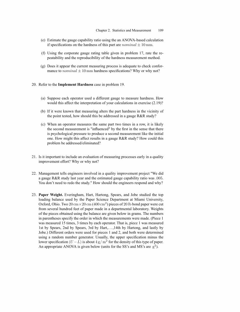
Chapter 2. Statistics and Measurement 109
(e) Estimate the gauge capability ratio using the an ANOVA-based calculationif speci�cations on the hardness of this part are nominal � 10mm.
(f) Using the corporate gauge rating table given in problem 17, rate the re-peatability and the reproducibility of the hardness measurement method.
(g) Does it appear the current measuring process is adequate to check confor-mance to nominal � 10mm hardness speci�cations? Why or why not?
20. Refer to the Implement Hardness case in problem 19.
(a) Suppose each operator used a different gauge to measure hardness. Howwould this affect the interpretation of your calculations in exercise (2.19)?
(b) If it were known that measuring alters the part hardness in the vicinity ofthe point tested, how should this be addressed in a gauge R&R study?
(c) When an operator measures the same part two times in a row, it is likelythe second measurement is "in�uenced" by the �rst in the sense that thereis psychological pressure to produce a second measurement like the initialone. How might this affect results in a gauge R&R study? How could thisproblem be addressed/eliminated?
21. Is it important to include an evaluation of measuring processes early in a qualityimprovement effort? Why or why not?
22. Management tells engineers involved in a quality improvement project "We dida gauge R&R study last year and the estimated gauge capability ratio was :005.You don't need to redo the study." How should the engineers respond and why?
23. Paper Weight. Everingham, Hart, Hartong, Spears, and Jobe studied the toploading balance used by the Paper Science Department at Miami University,Oxford, Ohio. Two 20 cm�20 cm (400 cm2) pieces of 20 lb bond paper were cutfrom several hundred feet of paper made in a departmental laboratory. Weightsof the pieces obtained using the balance are given below in grams. The numbersin parentheses specify the order in which the measurements were made. (Piece 1was measured 15 times, 3 times by each operator. That is, piece 1 was measured1st by Spears, 2nd by Spears, 3rd by Hart,. . . ,14th by Hartong, and lastly byJobe.) Different orders were used for pieces 1 and 2, and both were determinedusing a random number generator. Usually, the upper speci�cation minus thelower speci�cation (U�L) is about 4 g=m2 for the density of this type of paper.An appropriate ANOVA is given below (units for the SS's and MS's are g2).
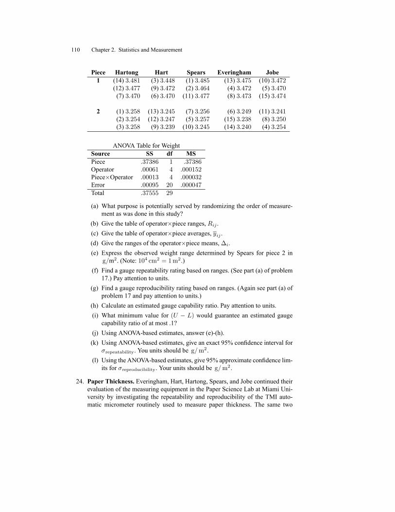
110 Chapter 2. Statistics and Measurement
Piece Hartong Hart Spears Everingham Jobe1 (14) 3:481 (3) 3:448 (1) 3:485 (13) 3:475 (10) 3:472
(12) 3:477 (9) 3:472 (2) 3:464 (4) 3:472 (5) 3:470(7) 3:470 (6) 3:470 (11) 3:477 (8) 3:473 (15) 3:474
2 (1) 3:258 (13) 3:245 (7) 3:256 (6) 3:249 (11) 3:241(2) 3:254 (12) 3:247 (5) 3:257 (15) 3:238 (8) 3:250(3) 3:258 (9) 3:239 (10) 3:245 (14) 3:240 (4) 3:254
ANOVA Table for WeightSource SS df MSPiece :37386 1 :37386Operator :00061 4 :000152Piece�Operator :00013 4 :000032Error :00095 20 :000047Total :37555 29
(a) What purpose is potentially served by randomizing the order of measure-ment as was done in this study?
(b) Give the table of operator�piece ranges, Rij .(c) Give the table of operator�piece averages, yij .(d) Give the ranges of the operator�piece means,�i.(e) Express the observed weight range determined by Spears for piece 2 in
g=m2. (Note: 104 cm2 = 1m2:)(f) Find a gauge repeatability rating based on ranges. (See part (a) of problem17.) Pay attention to units.
(g) Find a gauge reproducibility rating based on ranges. (Again see part (a) ofproblem 17 and pay attention to units.)
(h) Calculate an estimated gauge capability ratio. Pay attention to units.(i) What minimum value for (U � L) would guarantee an estimated gaugecapability ratio of at most .1?
(j) Using ANOVA-based estimates, answer (e)-(h).(k) Using ANOVA-based estimates, give an exact 95% con�dence interval for
�repeatability. You units should be g=m2:(l) Using the ANOVA-based estimates, give 95% approximate con�dence lim-its for �reproducibility. Your units should be g=m2:
24. Paper Thickness. Everingham, Hart, Hartong, Spears, and Jobe continued theirevaluation of the measuring equipment in the Paper Science Lab at Miami Uni-versity by investigating the repeatability and reproducibility of the TMI auto-matic micrometer routinely used to measure paper thickness. The same two

Chapter 2. Statistics and Measurement 111
20 cm � 20 cm pieces of 20 lb bond paper referred to in problem 23 were usedin this study. But unlike measuring weight, measuring thickness alters the prop-erties of the portion of the paper tested (by compressing it and thus changingthe thickness). So, an 8 � 8 grid was marked on each piece of paper. The cor-responding squares were labeled 1; 2; : : : ; 64 left to right, top to bottom. Tensquares from a given piece were randomly allocated to each operator (50 squaresfrom each piece were measured). Because so many measurements were to bemade, only the "turn" for each analyst was determined randomly, and each oper-ator made all 10 of his measurements on a given piece consecutively. A secondrandomization and corresponding order of measurement was made for piece 2.Hartong measured 3rd on piece 1 and 5th on piece 2, Hart was 1st on piece1 and 3rd on piece 2, Spears was 5th and 4th, Everingham was 2nd and 2nd,and Jobe was 4th and 1st. The data follow (in mm). The numbers in parenthe-sis identify the squares (from a given piece) measured. (Thus, for piece 1, Hartbegan the measurement procedure by recording thicknesses for squares 51, 54,18, 63; : : : ; 7, then Everingham measured squares 33; 38; : : : ; 5, etc. After thedata for piece 1 were obtained, measurement on piece 2 began. Jobe measuredsquares 9; 3; : : : ; 22 then Everingham measured squares 43; 21; : : : ; 57, etc.) Anappropriate ANOVA is also given (units for the SS's and MS's are mm2):
Piece Hartong Hart Spears Everingham Jobe1 (14) :201 (51) :195 (48) :192 (33) :183 (43) :185
(25) :190 (54) :210 (58) :191 (38) :189 (40) :204(17) :190 (18) :200 (15) :198 (36) :196 (49) :194(21) :194 (63) :203 (55) :197 (3) :195 (12) :199(53) :212 (20) :196 (44) :207 (59) :192 (29) :192(16) :209 (50) :189 (23) :202 (45) :195 (13) :193(47) :208 (31) :205 (64) :196 (41) :185 (56) :190(42) :192 (37) :203 (57) :188 (9) :193 (2) :195(22) :198 (34) :195 (26) :201 (62) :194 (8) :199(35) :191 (7) :186 (1) :181 (5) :194 (6) :197
2 (5) :188 (14) :186 (55) .177 (43) :179 (9) :191(16) :173 (24) :171 (51) :174 (21) :194 (3) :180(11) :188 (62) :178 (36) :184 (18) :187 (42) :194(47) :180 (34) :175 (12) :180 (39) :175 (50) :183(25) :178 (29) :183 (38) :179 (6) :173 (53) :181(15) :188 (10) :185 (41) :186 (7) :179 (17) :188(56) :166 (30) :190 (63) :183 (64) :171 (33) :188(26) :173 (40) :177 (45) :172 (54) :184 (23) :173(8) :175 (58) :184 (31) :174 (59) :181 (60) :180(52) :183 (13) :186 (2) :178 (57) :187 (22) :176

112 Chapter 2. Statistics and Measurement
ANOVA Table for ThicknessSource SS df MSPiece :00557 1 :00557Operator :00018 4 :000045Piece�Operator :00028 4 :00007Error :003986 90 :000044Total :010013 99
(a) Say what each term in equation (2.25) means in the context of this problem.(b) How is this study different from a "garden variety" gauge R&R study?(c) Will the nonstandard feature of this study tend to increase, decrease, or
have no effect on the estimate of the repeatability standard deviation?Why?(d) Will the nonstandard feature of this study tend to increase, decrease, or
have no effect on the estimated standard deviation of measurements froma given piece across many operators? Why?
(e) Give the ANOVA-based estimated standard deviation of paper thicknessmeasurements for a �xed piece�operator combination, i.e., approximatethe repeatability standard deviation assuming that square-to-square varia-tion is negligible.
(f) Give the ANOVA-based estimated standard deviation of thicknesses mea-sured on a �xed piece across many operators. (The quantity being estimatedshould include but not be limited to variability for a �xed piece�operatorcombination.) That is, approximate the reproducibility standard deviationassuming square-to-square variation is negligible.
(g) What percent of the overall measurement variance is due to repeatability?What part is due to reproducibility?
25. Paper Burst Strength. An important property of �nished paper is the force( lb= in2) required to burst or break through it. Everingham, Hart, Hartong, Spears,and Jobe investigated the repeatability and reproducibility of existing measure-ment technology for this paper property. AMullen tester in the Miami UniversityPaper Science Department was studied. Since the same two 20 cm�20 cm piecesof paper referred to in problems 23 and 24 were available, the team used them inits gauge R&R study for burst strength measurement. The burst test destroys theportion of paper tested, so repeat measurement of exactly the same paper spec-imen is not possible. Hence, a grid of 10 approximately equal-sized rectangles,10 cm� 4 cm (each large enough for the burst tester), was marked on each largepaper piece. Each of the analysts was assigned to measure burst strength on tworandomly selected rectangles from each piece. The measurement order was alsorandomized among the �ve operators for each paper piece. The data obtained arebelow. The ordered pairs (a; b) specify the rectangle measured and the order ofmeasurement. (For example, the ordered pair (2,9) in the top half of the table in-dicates that 8:8 lb= in2 was obtained from rectangle number 2, the 9th rectanglemeasured from piece 1.) An ANOVA table for this study is also provided.

Chapter 2. Statistics and Measurement 113
Piece Hartong Hart Spears Everingham Jobe1 (9,2) 13:5 (6,6) 10:5 (4,8) 12:9 (2,9) 8:8 (3,10) 12:4
(7,5) 14:8 (5,1) 11:7 (1,4) 12:0 (8,3) 13:5 (10,7) 16:0
2 (3,9) 11:3 (1,8) 14:0 (5,6) 13:0 (6,7) 12:6 (2,1) 11:0(8,10) 12:0 (7,5) 12:5 (9,3) 13:1 (4,2) 12:7 (10,4) 10:6
ANOVA Table for Burst StrengthSource SS df MSPiece :5445 1 :5445Operator 2:692 4 :6730Piece�Operator 24:498 4 6:1245Error 20:955 10 2:0955Total 48:6895 19
In the following, assume that specimen-to-specimen variation within a givenpiece of paper is negligible.
(a) To what set of operators can the conclusions of this study be applied?(b) To what set of paper pieces can the conclusions of this study correctly be
applied?(c) What are the values of I , J , andm in this study?(d) Give an ANOVA-based estimate of the repeatability standard deviation, �.(e) Give another estimate of the repeatability standard deviation, �, this time
based on ranges.(f) Find an ANOVA-based estimate of �reproducibility.(g) Find another estimate of �reproducibility, this one based on ranges(h) Estimate the standard deviation of single burst measurements on a �xed
piece of paper made by many operators, �R&R.
26. Paper Tensile Strength. The �nal type of measurement method studied by Ever-ingham, Hart, Hartong, Spears, and Jobe in the Paper Science Lab at MiamiUniversity was that for paper tensile strength. Since the burst tests discussed inproblem 25 destroyed the 20 cm� 20 cm pieces of 20 lb bond paper referred tothere, two new 20 cm� 20 cm pieces of paper were selected from the same runof paper. Ten 15mm � 20 cmstrips were cut from each 20 cm � 20 cm piece.Each set of ten strips was randomly allocated among the �ve operators (2 stripsper operator for each set of ten). The order of testing was randomized for the tenstrips from each piece, and the same Thwing-Albert Intellect 500 tensile testerwas used by each operator to measure the load required to pull apart the strips.The data appear below in kg. (Consider, for example, the data given for piece1, Hartong, (9,2) 4.95. A 4.95 kg load was required to tear strip number 9 from

114 Chapter 2. Statistics and Measurement
piece 1 and the measurement was taken second in order among the ten stripsmeasured for piece 1.) Since the testing destroyed the strip, the analysts had toassume strip-to-strip variation for a given piece to be negligible. An appropriateANOVA is also given below (units for SS's and MS's are kg2).
Piece Everingham Hart Hartong Spears Jobe1 (2,8) 4:34 (1,5) 4:34 (9,2) 4:95 (6,6) 4:03 (10,4) 4:51
(8,10) 4:71 (4,3) 4:61 (7,7) 4:53 (3,9) 3:62 (5,1) 4:56
2 (4,7) 5:65 (6,6) 4:80 (1,1) 4:38 (2,2) 4:65 (9,5) 4:30(8,9) 4:51 (10,8) 4:75 (3,3) 3:89 (5,4) 5:06 (7,10) 3:87
ANOVA Table for Tensile StrengthSource SS df MSPiece :13778 1 :1378Operator :69077 4 :17269Piece�Operator 1:88967 4 :47242Error 1:226 10 :1226
Total 3:9442 19
(a) Make a table of load averages, yij , for the 10 operator�piece combina-tions.
(b) Plot the load averages yij versus piece number for each of the operators(connect the two yij's for each operator).
(c) Suppose the target tensile strength for strips of 20 lb bond paper is 4:8 kg.Typically, upper and lower speci�cations for paper properties are set 5%above and below a target. Estimate the gauge capability ratio under theseconditions, using ANOVA-based calculations.
(d) If upper and lower speci�cations for tensile strength of 20 lb bond paperare equal distances above and below a target of 4.8 kg, �nd the upper andlower limits such that the estimated gauge capability ratio is .01.
(e) Redo part (d) for an estimated gauge capability ratio of .1.
(f) Is it easier to make a gauge capability ratio better (smaller) by increasingits denominator or decreasing its numerator? Will your answer lead to amore consistent �nal product? Why or why not?
27. Thorium Detection. In the article "Limits for Qualitative Detection and Quanti-tative Determination," which appeared in Analytical Chemistry in 1968, L. Cur-rie reported some experimental observations in the spectrophotometric determi-nation of thorium using thorin. The response variability from measurements on"blank" material was observed to be essentially the same as that from any (�xed)sample of interest, and extensive analysis of blank material produced a standard
Chapter 2. Statistics and Measurement 115
deviation of measurement (�measurement) of around .002. The absorbance re-sponse for a �eld sample is typically expressed as the measured response minusthat of a blank, and in these terms a response for a particular sample of interestwas .006.
(a) If an analyst is willing to tolerate a 5% risk of incorrectly concluding thata sample contains more thorium than is present in blank material, give thecritical limit Lc. For the sample mentioned above, what conclusion doesone reach using this critical limit? (Here, both nnew and nold are 1.)
(b) Suppose one can tolerate only a 1% chance of incorrectly concluding thereis more thorium in a sample than in a blank. Give the corresponding criticallimit and say what conclusion would be reached about a sample with aresponse of ynew = yold + :006.
(c) What risk level corresponds to a critical limit of .006?(d) What model assumptions must be made in order to answer (a) through (c)?(e) Suppose one can tolerate a 5% risk of incorrectly concluding a sample
contains more thorium than a blank and the critical value from (a) willbe employed. What is the value A (expressed in terms of an excess overthe mean value for a blank) such that the chance of not detecting a meanabsorbance of at least A (and corresponding thorium content above that ofthe blank material) is only 5%?
(f) In the vocabulary of Section 2.6 what is A in part (e)?
28. Refer to the Thorium Detection case in problem 27.
(a) Consider part (e) in problem 27. Another analyst can tolerate only a 1%risk for both types of possible errors. Find A for this analyst.
(b) Currie stated that the calibration factor used to translate absorbance read-ings to concentration values for thorium is about k = 58:2 l= g. (An ab-sorbance value divided by k gives a corresponding concentration.) Expressyour value for part (e) of problem 27 in � g= l. (Note that 1� g is 10�6 g.)
(c) Express your answer to part (a) of this problem in � g= l.(d) Find an increase in thorium concentration (over that in a blank) that is 10
times the standard deviation of the difference in a �eld sample reading anda blank reading (that is, 10�measurement
p1 + 1). Express your answer in
absorbance units and then in � g= l.
29. Carbon Atmospheric Blank. Currie, et al. presented the paper "Impact of theChemical and Isotopic Blank on the Interpretation of Environmental Radiocar-bon Results" at the International Radiocarbon Conference in Glasgow, Scotland,August 1994. Part of their presentation included discussion of six carbon con-tent measurements made on a single urban atmospheric aerosol �eld �lter blank.These six responses (in � g) were (in the order produced)

116 Chapter 2. Statistics and Measurement
95:6; 73:1; 56:9; 114:4; 42:3; and 35:6:
(a) Give an estimate of �measurement (using a sample standard deviation). Usethis estimate in the balance of this problem as if it were exactly �measurement.
(b) Assuming measured carbon follows a normal distribution, �nd a criticallimit, Lc, for determining whether a single measurement from a �eld sam-ple indicates a carbon content in excess of that in a blank (that will also bemeasured once). Use 2.5% for the probability of incorrectly deciding thatthere is more carbon in the �eld sample than in the blank.
(c) What additional assumption (beyond normality) must hold for your answerin (b) to be valid?
(d) Suppose now that every blank has the same and known amount of carbon.Using your answer to (a) as the standard deviation of a single �eld samplemeasurement, �nd a critical limit for deciding if the average of two mea-surements on a �eld sample indicates carbon in excess of that in any blank.Use 1% as the largest risk of incorrectly deciding that the sample containsexcess carbon that can be tolerated. (The intention here is that nnew = 2and nold =1.)
(e) Find a lower limit of detection based on your estimate in (a). In makingthis calculation use a 5% risk of incorrectly concluding a �eld sample con-tains more carbon than a blank (of unknown content). Also use 5% for theprobability that a �eld sample at the lower limit of detection will fail toproduce a difference exceeding the critical value. (Suppose that both the�eld sample and the blank will be measured once.)
(f) Let the two risks in (e) be 2.5%. Find a lower limit of detection.(g) As the two risk levels decrease, what happens to the lower limit of detec-
tion? Explain in the context of this problem.
30. Refer to theCarbon Atmospheric Blank case in problem 29. As in problem 29,assume that the estimate from part (a) is in fact exactly equal to �measurement.
(a) Find the increase in carbon content that is 10 times the (estimated) standarddeviation of the difference between the measured carbon content for a sin-gle �eld sample and that from a single blank. (That is, �nd 10�measurement
p1 + 1.)
(b) Suppose many measurements from the same blank are available. Answerpart (a) under these new conditions, if the difference of interest is that be-tween a single �eld sample measurement and the average of the large num-ber of measurements on a single blank. (That is, �nd 10�measurement
q1 + 1
1 .)
(c) Does knowing the true carbon content of a blank affect the lower limit ofdetection? Why or why not? (Hint: consider a single �eld sample measure-ment and a single blank measurement. Find the lower limit of detection us-ing, say, 5% risks. Compute lower limits of detection both when the blank

Chapter 2. Statistics and Measurement 117
content is considered to be known and then when it is unknown. Knowingthe true content of a blank means that nold =1. )
31. Dimethyl Phenanthrene (DMP4) Atmospheric Blank. The presentation re-ferred to in problem 29 also included a discussion of six measurements of theDMP4 content of an atmospheric �eld �lter blank. (DMP4 is a product of soft-wood pyrolysis.) The six responses in nanograms (10�9 g) were
8:25; 7:30; 7:27; 6:54; 6:75 and 7:32 :
(a) Suppose the �rst two measurements above were taken by operator 1, thesecond two by operator 2, and the last two readings by operator 3, butthe same blank and measuring instrument were involved in each of thethree pairs of measurements. Find an appropriate range-based estimate of�measurement = �R&R: In the rest of this problem use this estimate as if itwere perfect. (Hint: �R&R=
q�2repeatability + �
2reproducibility.)
(b) Find a critical limit, Lc, if the probability of a false positive is to be 10%and a randomly selected analyst is to measure a single response on both a�eld sample and a new blank.
(c) Continuing with the scenario in (a), �nd a lower limit of detection wherethe probability of a false positive detection is 10% and the probability of afalse negative is 5% for true content at the lower limit of detection.
32. In the context of Section 2.6, consider a situation where the probabilities of botha false positive and a false negative (when the new mean is at the lower limit ofdetection) are set at .05.
(a) Make a 2 � 2 table giving formulas for critical limits in column 1 andformulas for lower limits of detection in column 2, where row 1 in thetable corresponds to the case of one measurement from a �eld sample andone from a blank and row 2 in the table corresponds to one measurementfrom a �eld sample and a large number from a single blank.
(b) Add an additional column to the table in (a). Fill in this column with ex-pressions for 10 times the standard deviation of y�eld � yblank.
33. Lab Carbon Blank. The following data were provided by L. A. Currie of theNational Institute of Standards and Technology (NIST). The data are prelimi-nary and exploratory, but real. The unit of measure is "instrument response" andis approximately equal to 1� g of carbon. That is, 5:18 corresponds to 5:18 in-strument units of carbon or about 5:18� g of carbon. The responses come fromblank material generated in the lab.

118 Chapter 2. Statistics and Measurement
Test Number 1 2 3 4 5 6 7Measured Carbon 5:18 1:91 6:66 1:12 2:79 3:91 2:87
Test Number 8 9 10 11 12 13 14Measured Carbon 4:72 3:68 3:54 2:15 2:82 4:38 1:64
(a) Plot measured carbon content versus order of measurement.(b) The data are ordered in time, but intervals between measurements are not
equal and an appropriate plan for obtaining data was not necessarily inplace. What feature of the plot in (a) might still have meaning?
(c) If one treats the measurement of lab-generated blank material as repeatedmeasurements of a single blank, what does a trend on a plot like that in(a) suggest regarding �repeatability? (Assume the plot is made from dataequally spaced in time and collected by a single individual.)
(d) Make a frequency histogram of these data with categories 1:00� 1:99,2:00� 2:99, etc.
(e) What could be missed in a gauge R&R study if order of measurement wasimportant (and one didn't make a plot like that in (a)) for data like these?

This is page 119Printer: Opaque this
CHAPTER3
Process Monitoring
This chapter discusses the important topic of process monitoring using so-called "con-trol charts." These are devices for the routine and organized plotting of process per-formance measures, with the goal of identifying process changes. When these aredetected, those running the process can either intervene and set things aright (if thechange is detrimental) or try to make permanent the source of an unexpected processimprovement.The discussion begins with some control charting philosophy. Then the standard
Shewhart control charts for both measurements/"variables data" and counts/"attributesdata" are presented in consecutive sections. A fourth section discusses qualitative in-terpretation and practical implications of patterns sometimes seen on Shewhart charts,and some sets of rules often applied to check for such patterns. Then there is a pre-sentation of the so-called Average Run Length concept that can be used to quantifywhat a particular process monitoring scheme can be expected to provide. Finally, thechapter closes with a section clarifying the relationship between "statistical processcontrol" and "engineering control" and presenting some basic concepts of so-calledPID engineering control schemes.
3.1 Generalities About Shewhart Control ChartingSection 1.2.1 introduced the notion of process "stability" as consistency over time inthe pattern of process variation. Walter Shewhart, working at Bell Labs in the late1920s and early 1930s, developed an extremely powerful and simple tool for investi-gating whether a process can be sensibly thought of as stable. He called it a "control

120 Chapter 3. Process Monitoring
chart." Nearly 80 years after the fact, your authors would prefer (for reasons laid out inSection 3.6) that Shewhart had chosen instead the name "monitoring chart." Neverthe-less, this book will use Shewhart's terminology and the "monitoring chart" terminologyinterchangeably.Shewhart's fundamental conceptualization was that while some variation is inevitable
in any real process, overall variation seen in process data can be decomposed asShewhart'sGrandConceptualization
observed variation = baseline variation+ variation that can be eliminated : (3.1)
Shewhart conceived of baseline variation as that variability in production and measure-ment which will remain even under the most careful process monitoring and appropri-ate physical intervention. It is an inherent property of a combination of system con�g-uration and measurement methodology that cannot be reduced without basic changesin the physical process or how it is run or observed. This variation is sometimes calledvariation due to "system" or "common" (universal) causes. Other names for it that willbe used in this book are "random" or "short-term" variation. It is the kind of vari-ation expected under the best of circumstances, measuring item-to-consecutive-itemproduced on a production line. It is variation that comes from many small, unname-able, and unrecognized physical causes. When only this kind of variation is present,it is reasonable to call a process "stable" and model observations on it as independentrandom draws from a �xed population or universe.The second component of overall variability portrayed in equation (3.1) is that which
can potentially be eliminated by careful process monitoring and wise physical inter-vention (when such is warranted). This has variously been called "special cause" or"assignable" cause variation, "nonrandom" and "long-term" variation. It is the kind ofsystematic, persistent change that accompanies real (typically unintended) physical al-teration of a process (or the measurement system used to observe it). It is change that islarge enough that one can potentially track down and eliminate its root cause, leavingbehind a stable process.If one accepts Shewhart's conceptualization (3.1), the problem then becomes one of
detecting the presence of the second kind of variation so that appropriate steps can betaken to eliminate it. The Shewhart control chart is a tool for making such detection.The basic working of Shewhart's charting method is this. One periodically takes
samples from the process of interest (more will be said later about the timing and na-ture of these samples) and computes a statistic meant to summarize process behaviorat the period in question. Values of the statistic are plotted against time order of ob-servation and compared to so-called control limits drawn on the chart. These separate
Control Limits values of the statistic that are plausible if the process is in fact stable, from those thatare rare or implausible under this scenario. As long as the plotted points remain insidethe control limits, one presumes that all is well (the process is stable) and does notintervene in its workings. (This is an oversimpli�cation of how these charts are oftenused that will be corrected in Section 3.4. But for the time being this simpli�ed pic-ture will suf�ce.) When a point plots outside control limits, there is an indication thata physical change has probably taken place and that intervention is appropriate. Fig-ure 3.1 shows a generic Shewhart control chart where the plotted statistic is Q, upper

Chapter 3. Process Monitoring 121
and lower control limits are UCLQ and LCLQ respectively, and there is one "out ofcontrol" point.
FIGURE 3.1. Generic Shewhart control chart (for a statistic Q)
There are many different kinds of Shewhart charts, corresponding to various choicesof the plotted statistic, Q. Some of these chart types will be discussed in the next twosections. But before moving to discussion of speci�c charts, several generalities remainto be considered. First, there is the question of how one sets the control limits, UCLQand LCLQ.Shewhart's suggestion for setting control limits was essentially the following. If
one can model the process output under stable conditions (i.e., if one can specify asensible probability distribution for individual observations made on the process) thenprobability theory can often be invoked to produce a corresponding distribution forQ. Then small upper and lower percentage points for this distribution can providethe necessary control limits. The thinking is that only rarely will values outside thesebe seen under stable process conditions. Further, rather than working explicitly withprobability tables or formulas for a distribution of Q, one often simply makes use ofthe fact that for many probability distributions most of the probability is within threestandard deviations of the mean. So, if �Q and �Q are respectively a stable-processmean and standard deviation for Q, then common control limits are
Generic3-sigmaControl Limits
UCLQ = �Q + 3�Q and LCLQ = �Q � 3�Q : (3.2)
Further, it is common to draw in a "center line" on a Shewhart control chart at
GenericCenter LineCLQ = �Q : (3.3)
To make this discussion slightly more concrete, consider brie�y the situation wherethe plotted statistic is the sample mean of n individual measurements, Q = x. If theprocess output can be modeled as independent selections from a distribution with mean� and standard deviation �, the statistic x has a distribution with mean �Q = �x = �

122 Chapter 3. Process Monitoring
and standard deviation �Q = �x = �=pn. Then applying relationships (3.2) and (3.3)
it follows that typical control limits for x are
UCLx = �+ 3�pn
and LCLx = �� 3�pn, (3.4)
with a center line drawn at �.Display (3.4) helps bring into focus another general issue regarding Shewhart con-
trol charting. As in limits (3.4), process parameters (like � and �) typically appear informulas for control limits. Values for them must come from somewhere in order toapply a control chart, and there are two possibilities in this regard. Sometimes past
StandardsGiven Context
experience with a process, engineering standards, or other considerations made priorto process monitoring specify what values should be used. This kind of situation iscommonly known as a standards given scenario. In other circumstances, one has noinformation on a process outside a series of samples that are presented along with thequestion "Is it plausible that the process was physically stable over the period repre-sented by these data?" In such a case, all that one can do is tentatively assume thatin fact the process was stable, make provisional estimates of process parameters andplug them into formulas for control limits, and apply those limits to the data in handas a means of criticizing the tentative assumption of stability. This kind of situation is
RetrospectiveContext
sometimes called an as past data scenario, and will often be referred to in this text asa retrospective scenario.The difference between what is possible in standards given and retrospective con-
texts can be thought of in terms of two different questions addressed in the two situa-tions. In a standards given context, with each new sample one can face the question
"Are process parameters currently at their standard values?"
In a retrospective context, one can only wait until a number of samples have beencollected (often, a minimum of 20�25 time periods is recommended) and then lookingback over the data ask the question
"Are these data consistent with any �xed set of process parameters?"
Having introduced the notion of control limits, it is important to warn readers ofa common pitfall. That is the confusion that students (and even practicing engineers)often have regarding the much different concepts of control limits and engineeringspeci�cations. Control limits have to do with assessing process stability. They refer
Control Limitsvs EngineeringSpeci�cations
to a statistic Q. They are usually derived from what a process has done in the pastor is currently doing. On the other hand, engineering speci�cations have to do withassessing product acceptability or functionality. They almost always refer to individualmeasurements. They are usually derived from product performance requirements, andmay have little or nothing to do with the inherent capability of a process to produce aproduct meeting those requirements.Despite these real differences in meaning, people often confuse these concepts (for
example, applying speci�cations to sample means as if they were control limits, or ar-guing that since a mean or individual is inside control limits for x, the product being

Chapter 3. Process Monitoring 123
monitored is acceptable). But it is vital that these notions be kept separate and appliedin their proper contexts. (Notice that a process that is stable and producing Q's in-side appropriate control limits need not be producing mostly acceptable product. Andconversely, a process may produce product that is acceptable by current engineeringstandards, but nevertheless be very unstable!)Another issue needing some general discussion here is the matter of sampling. How
should one go about gathering the data to be used in control charting? This matter in-cludes the issue sometimes referred to as rational subgrouping or rational sampling.When one is collecting process-monitoring data, it is important that anything one in-tends to call a single "sample" be collected over a short enough time span that thereis little question that the process was physically stable during the data collection pe-riod. It must be clear that an "independent draws from a single population/universe"model is appropriate for describing data in a given sample. This is because the vari-ation within such a sample essentially speci�es the level of background noise againstwhich one looks for process changes. If what one calls "samples" often contain datafrom genuinely different process conditions, the apparent level of background noisewill be so large that it will be hard to see important process changes. In high-volumemanufacturing applications of control charts, single samples (rational subgroups) typi-cally consist of n consecutive items taken from a production line. On the other hand, inextremely low-volume operations, where one unit might take many hours to produceand there is signi�cant opportunity for real process change between consecutive units,the only natural samples may be of size n = 1.Once one has determined to group only observations close together in time into
samples or subgroups, there is still the question of how often these samples should betaken. When monitoring a machine that turns out 1000 parts per hour, where samplesare going to consist of n = 5 consecutive parts produced on the machine, does onesample once every minute, once every hour, once every day, or what? An answer tothis kind of question depends upon what one expects in terms of process performance,and the consequences of process changes. If the consequences of a process changeare disastrous, one is pushed toward frequent samples. The same is true if signi�cantprocess upsets are a frequent occurrence. On the other hand, if a process rarely expe-riences changes and even when those occur only a moderate loss is incurred when ittakes a while to discover them, long intervals between samples are sensible. Variousoperations-research type attempts have been made to provide quantitative guidelinesin answer to this sampling frequency question, but these have proved largely unsatis-factory for practice. But the qualitative matters noted here clearly need to be the majorconsiderations as looks for an appropriate sampling frequency for process monitoring.As a �nal matter in this introductory discussion of Shewhart charting philosophy we
should say what control charting can and cannot reasonably be expected to provide.It can signal the need for process intervention and can keep one from ill-advised anddetrimental over-adjustment of a process that is behaving in a stable fashion. But indoing so, what is achieved is simply reducing variation to the minimum possible fora given system con�guration (in terms of equipment, methods of operation, methodsof measurement, etc.). Once that minimum has been reached, what is accomplished

124 Chapter 3. Process Monitoring
is maintaining a status quo best possible process performance. (Remember, for exam-ple, the use of the "control" step in the six-sigma paradigm discussed on page 10.) Intoday's global economy, standing still is never good enough for very long. Achievingprocess stability provides a solid background against which to evaluate possible in-novations and fundamental/order-of-magnitude improvements in production methods.But it does not itself guide their discovery. Of the tools discussed in this book, it is themethods of experimental design and analysis covered in Chapters 5 and 6 that have themost to say about aiding fundamental innovations.
Section 3.1 Exercises1. What can control charting contribute to a process improvement effort?
2. What is the difference between "standards given" and "retrospective" controlcharting?
3. What is the difference between common cause and special cause variation?Which type of variation are control charts designed to detect?
4. What happens to the control limits (3.4) for an x chart as the subgroup size getslarge?
5. How do you expect the behavior of a control charting scheme to change if avalue smaller than 3 is used in limits (3.2)?
6. How do you expect the behavior of a control charting scheme to change if avalue larger than 3 is used in limits (3.2)?
7. If the plotted statistic Q is inside appropriately constructed control limits (indi-cating that a process is stable), does that necessarily imply that the process isproducing acceptable product? Brie�y explain.
8. If the plotted statistic Q is regularly outside appropriately constructed controllimits (indicating that a process is unstable), does that necessarily imply that theprocess is producing unacceptable product? Brie�y explain.
9. The same item is being produced on two production lines. Every 15 minutes 5items are sampled from each line and a feature of interest is measured on eachitem. Some statistic Q is calculated for each set of 5 measurement from each lineand plotted versus time. Analyst 1 puts all 10 items together into a single group(5 from line 1 and 5 from line 2), calculates a value of the statistic Q and plots it.(This person says, "After all, isn't a larger sample size better?") Analyst 2 keepsthe data from the two different lines separate and makes a different control chartfor each production line.
(a) What subgroup size is Analyst 1 using?

Chapter 3. Process Monitoring 125
(b) What subgroup size is Analyst 2 using?
(c) Which analyst is making the most appropriate chart?Why? (Hint: Considerthe concept of rational subgrouping.)
3.2 Shewhart Charts forMeasurements/"Variables Data"This section considers the problem of process monitoring when the data available aremeasurements (as opposed to counts or the kind of 0=1 calls considered in Section 2.7).Sometimes the terminology "variables data" is used in this context. In such situations, itis common to make charts for both the process location and also for the process spread(size of the process short-term variability). So this section will consider the making ofx and median (~x) charts for location, and R and s charts for spread.
3.2.1 Charts for Process LocationThe most common of all Shewhart control charts is that for means of samples of nmeasurements, the case where Q = x. As was discussed in the previous section (andportrayed in display (3.4)), the fact that sampling from a distribution with mean �and standard deviation � produces sample averages with expected value �x = � andstandard deviation �x = �=
pn suggests standards given Shewhart control limits for
x
StandardsGiven x ChartControl Limits
UCLx = �+ 3�pn
and LCLx = �� 3�pn; (3.5)
and center line at
StandardsGiven x ChartCenter Line
CLx = � :
Example 25 Monitoring the Surface Roughness of Reamed Holes. Dohm, Hong,Hugget, and Knoot worked with a manufacturer on a project involving roughness mea-surement after the reaming of preformed holes in a metal part. Table 3.1 contains somesummary statistics (the sample mean x, the sample median ~x, the sample rangeR, andthe sample standard deviation s) for 20 samples (taken over a period of 10 days) ofn = 5 consecutive reamed holes.

126 Chapter 3. Process Monitoring
Suppose for the time being that standards (established on the basis of previous expe-rience with this reaming process) for surface roughness are � = 30 and � = 4. Then,standards given control limits for the x values in Table 3.1 are
UCLx = 30 + 34p5= 35:37
and
LCLx = 30� 34p5= 24:63 :
Figure 3.2 is a standards given x chart for the surface roughness measurements. Basedon this chart, one would detect the fact that the reaming process is not stable at stan-dard process parameters as early as the second sample. Several of the sample meansfall outside control limits, and had the control limits been applied to the data as theywere collected, the need for physical intervention would have been signaled.
FIGURE 3.2. Standards given x chart for surface roughness
In order to make a retrospective x chart one must derive estimates of the processparameters � and � from data in hand (temporarily assuming process stability) andplug them into the formulas (3.5). There are many possible ways of doing this, eachleading to slightly different retrospective control limits. Here only the most commonones will be considered and we begin with the matter of estimating �.Let r stand for the number of samples available in a retrospective x chart analysis.
One way of estimating a supposedly common process mean for the r periods is tosimply average the r sample means. Standard control charting practice is to use

Chapter 3. Process Monitoring 127
TABLE 3.1. Summary Statistics for 20 Samples of 5 Surface Roughness Measurements onReamed Holes (� in)
Sample x ~x R s1 34:6 35 9 3:42 46:8 45 23 8:83 32:6 34 12 4:64 42:6 41 6 2:75 26:6 28 5 2:46 29:6 30 2 0:97 33:6 31 13 6:08 28:2 30 5 2:59 25:8 26 9 3:210 32:6 30 15 7:511 34:0 30 22 9:112 34:8 35 5 1:913 36:2 36 3 1:314 27:4 23 24 9:615 27:2 28 3 1:316 32:8 32 5 2:217 31:0 30 6 2:518 33:8 32 6 2:719 30:8 30 4 1:620 21:0 21 2 1:0
AverageSample Meanx =
1
r
rXi=1
xi
as an estimator of � in making retrospective control limits for x.An answer to the question of how to estimate � is not quite so obvious. The estimator
of � with the best theoretical properties is obtained by pooling the r sample variancesto obtain (in the constant sample size case)
s2pooled =1
r
rXi=1
s2i ;
and then taking the square root. However, this method is not common in practice (dueto historical precedent). Instead, common practice is to use estimators based on theaverage sample range or the average sample standard deviation.Consider �rst the estimation of � based on

128 Chapter 3. Process Monitoring
AverageSample Range
R =1
r
rXi=1
Ri :
As in the discussion of range-based estimation in gauge R&R on page 67, if processoutput is normally distributed at time period i,
ERi = d2�
and thus
E
�Rid2
�= � :
(The dependence of d2 on n is not being displayed here, since there is no chance ofconfusion regarding which "sample size" is under discussion.) So assuming the processis stable over all r periods, all sample sizes are n, and that a normal distribution governsthe data generation process,
R
d2
is a sensible estimator of �. Plugging this and x into the standards given control limitsfor x provided in display (3.5) one obtains retrospective Shewhart control limits for x,
UCLx = x+ 3R
d2pn
and LCLx = x� 3R
d2pn: (3.6)
Further, one can de�ne a constant A2 (depending upon n) by
A2 =3
d2pn;
and rewrite display (3.6) more compactly as
RetrospectiveControl Limitsfor x Based onthe AverageRange
UCLx = x+A2R and LCLx = x�A2R : (3.7)
Values of A2 can be found in the table of control chart constants, Table A.1.As an alternative to estimating � on the basis of sample ranges, next consider esti-
mating � based on the average sample standard deviation,

Chapter 3. Process Monitoring 129
AverageSampleStandardDeviation
s =1
r
rXi=1
si :
When sampling from a normal distribution with standard deviation �, the sample stan-dard deviation, s, has a mean that is not quite �. The ratio of the mean of s to � iscommonly called c4. (c4 depends upon the sample size and again is tabled in TableA.1, but it will not be necessary to display the dependence of c4 on n.) Thus, if oneassumes that process output is normally distributed at period i,
E
�sic4
�= � :
So assuming the process is stable over all r periods, all sample sizes are n, and that anormal distribution governs the data generation process,
s
c4
is a sensible estimator of �. Plugging this and x into the standards given control limitsfor x provided in display (3.5) one obtains retrospective Shewhart control limits for x,
UCLx = x+ 3s
c4pn
and LCLx = x� 3s
c4pn: (3.8)
Further, one can de�ne another constant A3 (depending upon n) by
A3 =3
c4pn;
and rewrite display (3.8) more compactly as
RetrospectiveControl Limitsfor x Based onthe AverageStandardDeviation
UCLx = x+A3s and LCLx = x�A3s : (3.9)
Values of A3 can also be found in the table of control chart constants, Table A.1.
Example 26 (Example 25 continued.) Returning to the reaming study, from Table 3.1
x = 32:1; R = 8:95; and s = 3:76 :

130 Chapter 3. Process Monitoring
Further, for n = 5 (which was the sample size used in the study) Table A.1 shows thatA2 = :577 and A3 = 1:427. Thus, from formulas (3.7), retrospective control limits forx based on R are
UCLx = 32:1 + :577(8:95) = 37:26 and LCLx = 32:1� :577(8:95) = 26:94 :
And from formulas (3.9), retrospective control limits for x based on s are
UCLx = 32:1 + 1:427(3:76) = 37:47 and LCLx = 32:1� 1:427(3:76) = 26:73 :
Figure 3.3 shows the retrospective x control chart with control limits based on R. Itis clear from this chart (as it would be using the limits based on s) that the reamingprocess was not stable over the period of the study. The mean measured roughness�uctuated far more than one would expect under any stable process model.
FIGURE 3.3. Retrospective x chart for surface roughness
x charts are by far the most common charts for monitoring process location, butthere is an alternative worth mentioning. That is to use sample medians in place ofsample means (~x in place of x). This alternative has the advantage of requiring less inthe way of computational skills from those who must compute the values to be plotted,but has the drawback of being somewhat less sensitive to changes in process locationthan the x chart.The basic probability facts that lead to control limits for ~x concern sampling from a
normal distribution. For a sample of size n from a normal distribution with mean � andstandard deviation �, the random variable ~x has mean �~x = � and standard deviation�~x = ��x = ��=
pn for a constant � (depending upon n). Table 3.2 gives a few
values of �.Applying these facts about the probability distribution of ~x under a normal process
model and the generic Shewhart control limits given in display (3.2) produces stan-dards given control limits for ~x

Chapter 3. Process Monitoring 131
TABLE 3.2. Ratios � Between �~x and �x When Sampling from a Normal Distributionn 3 5 7 9 11 1� 1:160 1:197 1:214 1:223 1:229
p�=2
StandardsGiven ControlLimits forMedians
UCL~x = �+ 3��pn
and LCL~x = �� 3��pn: (3.10)
Retrospective limits can be made by replacing � and � with any sensible estimates.
Example 27 (Examples 25 and 26 continued.) Returning to the reaming study, sup-pose once more that process standards are � = 30 and � = 4. Then for samples ofsize n = 5 (like those used in the students' project) control limits for sample mediansare
UCL~x = 30 + 3(1:197)4p5= 36:42
andLCL~x = 30� 3(1:197)
4p5= 23:58 :
Had these limits been applied to the data of Table 3.1 as they were collected, the needfor physical intervention would have been signaled as early as the second sample.
3.2.2 Charts for Process SpreadOur exposition of control charts for measurements began with the x chart for loca-tion because it is surely the single most commonly used process monitoring tool, andbecause facts from elementary probability can be invoked to quickly motivate the no-tion of control limits for x. However, in practice it is often important to deal �rst withthe issue of consistency of process spread before going on to consider consistency ofprocess location. After all, such consistency of spread (constancy of �) is already im-plicitly assumed when one sets about to compute control limits for x. So it is importantto now consider charts intended to monitor this aspect of process behavior. The discus-sion here will center on charts for ranges and standard deviations, beginning with therange chart.In derivingR=d2 as an estimator of � we have employed the fact that when sampling
from a normal universe with mean � and standard deviation �,
ER = �R = d2� . (3.11)
The same kind of mathematics that stands behind relationship (3.11) can be used to alsoderive a standard deviation to associate with R. (This is a measure of spread for theprobability distribution ofR, which is itself a measure of spread of the sample.) It turns

132 Chapter 3. Process Monitoring
out that the standard deviation ofR is proportional to �. The constant of proportionalityis called d3 and is tabled in Table A.1. (Again, d3 depends on n, but it will not be usefulto display that dependence here.) That is,
�R = d3� : (3.12)
Now the relationships (3.11) and (3.12) together with the generic formula for She-whart control limits given in display (3.2) and center line given in display (3.3) implythat standards given control limits for R are
UCLR = (d2 + 3d3)� and LCLR = (d2 � 3d3)� (3.13)
with a center line at
StandardsGiven R ChartCenter Line
CLR = d2� : (3.14)
Further, if one adopts the notationsD2 = d2+3d3 andD1 = d2�3d3 the relationships(3.13) can be written somewhat more compactly as
StandardsGiven R ChartControl Limits
UCLR = D2� and LCLR = D1� : (3.15)
Values of the constants D1 and D2 may again be found in the table of control chartconstants, Table A.1.It is instructive to look at the tabled values of D1. There are no tabled values for
sample sizes n � 6. For such sample sizes the difference d2 � 3d3 turns out to benegative. Since ranges are nonnegative, a negative lower control limit would make nosense. So standard practice for n � 6 is to use no lower control limit for R.Consider also the implications of the fact that for n > 6, one typically employs
a positive lower control limit for R. This means that it is possible for an R chart tosignal an "out of control" situation because R is too small. This fact sometimes causesstudents consternation. After all, isn't the goal to produce small variation? Then whysignal an alarm when R is small? The answer to this conundrum lies in rememberingprecisely what a control chart is meant to detect, namely process instability/change. Itis possible for unintended causes to occasionally act on a process to reduce variability.A lower control limit on an R chart simply allows one to detect such happy events. Ifone can detect such a change and identify its physical source, there is the possibility ofmaking that assignable cause part of standard practice and the accompanying decreasein � permanent. So, the practice of using positive lower control limits for R when n issuf�ciently big is one that makes perfectly good practical sense.

Chapter 3. Process Monitoring 133
Example 28 (Examples 25 through 27 continued.) Consider once more the reamingexample of Dohm, Hong, Hugget, and Knoot from a standards given perspective with� = 4. For samples of size n = 5, Table A.1 provides the values d2 = 2:326 andD2 = 4:918. So using formulas (3.14) and (3.15), standards given control chart valuesfor R are
UCLR = 4:918(4) = 19:7 and CLR = 2:326(4) = 9:3 :
Figure 3.4 is the corresponding standards given control chart for the students' ranges.There are three out-of-control points on the chart, the �rst coming as early as the sec-ond sample. The reaming process did not behave in a manner consistent with the � = 4standard over the period of the study. Samples 2, 11, and 14 simply have too much in-ternal variability to make consistency of � at the value 4 believable. One wonders ifperhaps the reamer was changed in the middle of these samples, with the effect thatsome holes were very rough while others were very smooth.
FIGURE 3.4. Standards given R chart for surface roughness
Retrospective control limits forR come about by plugging an estimate for � derivedfrom samples in hand into the formulas (3.14) and (3.15). A particularly natural choicefor an estimator of � in this context is R=d2. Substituting this into relationship (3.14),one gets the perfectly obvious retrospective center line for an R chart,
RetrospectiveR ChartCenter Line
CLR = R : (3.16)
Further, substituting R=d2 into equations (3.15) for �, one gets retrospective controllimits for R
UCLR = D2�R
d2
�and LCLR = D1
�R
d2
�: (3.17)

134 Chapter 3. Process Monitoring
And adopting the notations D4 = D2=d2 and D3 = D1=d2, it is possible to write therelationships (3.17) more compactly as
RetrospectiveR ChartControl Limits
UCLR = D4R and LCLR = D3R : (3.18)
As is by now to be expected, the constantsD3 andD4 are tabled in Table A.1. And thetable contains no values of D3 for n � 6.
Example 29 (Examples 25 through 28 continued.) Recall that the 20 samples inTable 3.1 haveR = 8:95 and note that for n = 5,D4 = 2:114. So from displays (3.16)and (3.18) a retrospective control chart for the ranges (based on R=d2 as an estimatorof �) has center line at
CLR = R = 8:95and upper control limit
UCLR = D4R = 2:114(8:95) = 18:9 :
A plot of this retrospective R chart would look very little different from Figure 3.4. Thesame three ranges plot outside control limits. Not only is a "� constant at 4" view of thestudents' data not plausible, but neither is a "� constant at some value" view. There issolid evidence of reaming process instability in the ranges of Table 3.1. The short-termprocess variability changes over time.
The R chart is the most common Shewhart control chart for monitoring processspread. It requires very little from its user in the way of calculations, is based on astatistic that is very easy to understand, and is �rmly entrenched in quality assurancepractice dating from the days of Shewhart himself. There is, however, an alternative tothe R chart that tends to detect changes in process spread more quickly, at the price ofincreased computational complexity. Where the quantitative sophistication of a user ishigh and calculations are not a problem, the s chart is a viable competitor for the Rchart.The fact that (when sampling from a normal distribution)
Es = c4� ; (3.19)
has already proved useful when making retrospective control limits for x based on s.The same kind of mathematics that leads to relationship (3.19) can be used to �ndthe standard deviation of s (based on a sample from a normal universe). (This is ameasure of spread for the probability distribution of the random variable s, that isitself a measure of spread of the sample.) It happens that this standard deviation is amultiple of �. The multiplier is called c5 and it turns out that c5 =
p1� c24. That is,
�s = �q1� c24 = c5� : (3.20)

Chapter 3. Process Monitoring 135
Now relationships (3.19) and (3.20) together with the generic Shewhart control lim-its and center line speci�ed in displays (3.2) and (3.3) lead immediately to standardsgiven control limits and center line for an s chart. That is,
UCLs = (c4 + 3c5)� and LCLs = (c4 � 3c5)� (3.21)
and
StandardsGiven s ChartCenter Line
CLs = c4� : (3.22)
Further, if one adopts the notationsB6 = c4+3c5 andB5 = c4�3c5, the relationships(3.21) can be written as
StandardsGiven s ChartControl Limits
UCLs = B6� and LCLs = B5� : (3.23)
Values of the constants B5 and B6 may again be found in the table of control chartconstants, Table A.1. For n � 5 there are no values of B5 given in Table A.1 becausefor such sample sizes c4 � 3c5 is negative. For n > 5, B5 is positive, allowing the schart to provide for detection of a decrease in � (just as is possible with an R chart andn > 6).Retrospective control limits for s can be made by substituting any sensible estimate
of � into the standards given formulas (3.23) and (3.22). A particularly natural choicein this context is s=c4. Substituting this into relationship (3.23), one gets the obviousretrospective center line for an s chart
Retrospective sChart CenterLine
CLs = s : (3.24)
Further, substituting s=c4 into equations (3.23) for � produces retrospective controllimits for s
UCLs = B6�s
c4
�and LCLs = B5
�s
c4
�: (3.25)
And adopting the notations B4 = B6=c4 and B3 = B5=c4, it is possible to write therelationships (3.25) more compactly as

136 Chapter 3. Process Monitoring
Retrospective sChart ControlLimits
UCLs = B4s and LCLs = B3s : (3.26)
As usual, the constants B3 and B4 are tabled in Table A.1, and the table contains novalues of B3 for n � 5.
Example 30 (Examples 25 through 29 continued.) The 20 samples in Table 3.1 haves = 3:76. For n = 5; B4 = 2:089. So from displays (3.24) and (3.26) a retrospectivecontrol chart for the standard deviations (based on s=c4 as an estimator of �) hascenter line at
CLs = s = 3:76
and upper control limit
UCLs = B4s = 2:089(3:76) = 7:85 :
Figure 3.5 is a retrospective s chart for the sample standard deviations of Table 3.1.It carries the same message as does a retrospective analysis of the sample ranges forthis example. Not only is a "� constant at 4" view of the students' data not plausible,neither is a "� constant at some value" view. There is solid evidence of reaming processinstability in the standard deviations of Table 3.1.
FIGURE 3.5. Retrospective s chart for surface roughness
3.2.3 What if n = 1?To call n observations a "sample" or a "rational subgroup" is to implicitly guaranteethat they were collected under essentially constant process conditions. The discussionin Section 3.1 has already raised the possibility (particularly in some low volume pro-duction contexts) that a natural sample or subgroup size can be n = 1. Sometimes it is

Chapter 3. Process Monitoring 137
simply not safe to assume that even two successive process outcomes are necessarilygenerated under the same conditions.There are two commonly raised questions about control charting for measurements
when n = 1. These are
1. Exactly what should one chart (in particular, should one chart so-called "movingranges")? and
2. How does one estimate a process standard deviation, �?
We consider these questions before closing this section on Shewhart charting for mea-surements data.Where rational subgroups are of size n = 1 there is really only one possible choice
for a plotted statistic Q, namely x. One can "transform" the most natural measurementto some other scale (for example, by taking logarithms) but ultimately it is Q = xthat is available for plotting. However, people used to making x and R chart (or xand s chart) pairs in cases where n > 1 sometimes reason that it might be useful tosupplement an x chart (or individuals chart) with a chart on which one plots movingranges
Moving Rangefor an tthObservation, xi
MRi = jxi � xi�1j
The most commonly suggested version of this is where standards given control limitsfor x (the limits (3.5) for x when n = 1)
StandardsGiven ControlLimits forIndividuals, x
UCLx = �+ 3� and LCLx = �� 3� (3.27)
are used together withUCLMR = D2� (3.28)
(for D2 based on the pseudo-sample size of n = 2). This practice turns out to pro-duce a very large "false alarm rate" when in fact the process is stable. And attemptsto remedy this by applying control limits looser than (3.27) and (3.28) are typicallynot repaid with improved ability to detect process changes over what is available usingonly an x chart with limits (3.27). Adding a moving range chart to an individuals chartjust turns out to be a bad idea that should probably disappear from control chartingpractice. There is, to our knowledge, only one circumstance in which adding the mov-ing range chart to an individuals chart makes sense. That is a case where the departurefrom stable process behavior that one fears and needs to detect is one of oscillation

138 Chapter 3. Process Monitoring
in consecutive individuals. There, a moving range chart is (not surprisingly) more ef-fective than the individuals chart at "seeing" the non-standard process behavior. To be
Chart Only xWhen n = 1
absolutely explicit, in cases where n = 1, the best thing to do about control chartingis typically to use only an individuals chart with corresponding control limits (3.27).Consider then the second question above. When n = 1, there are no sample ranges
or standard deviations to use in estimating �. In fact, there is no really honest way to es-timate a process standard deviation unless one has a sample or samples with n � 2. Butsome "dishonest" methods are less dishonest than others, and the best known method(the least dishonest method) is based on an average of moving ranges of successiveobservations. (Notice that this is not a matter of process monitoring based on movingranges, but rather using moving ranges to estimate process standard deviation.)The rationale for using moving ranges of successive observations in estimating �
is this. If process conditions can change observation to observation, observations willvary not only because � 6= 0, but because the process mean changes. However, it isnot unreasonable to expect the variability in pairs of successive observations to be lessaffected by mean changes than the variability of any other type of group of observationsthat could be made up. It is thus reasonable to use moving ranges to make an estimate ofprocess standard deviation. While such an estimate is potentially in�ated by variationin the process mean, it can be expected to be less so than any other estimate one mightmake.The exact form of estimator of � we'll use (based on samples of size n = 1) is
Moving Range-Based Estimateof �
� =MR
d2(3.29)
where d2 is for "sample size" 2 (as there are 2 observations represented in each movingrange). This is a conservative estimator, as it will tend to over-estimate � when � is notconstant. But it is the best one available.
Example 31 A Numerical Example. Consider the 8 successive observations in thetable below and the corresponding 7 moving ranges.
Sample 1 2 3 4 5 6 7 8x 5 3 9 10 17 4 6 2MR 2 6 1 7 13 2 4
The values 5; 3; 9; 10; 17; 4; 6; 2 certainly vary because � 6= 0. They may vary be-yond what can be attributed to inherent process short term variability if � is not con-stant. That is, the 7 moving ranges should not be thought of as honest sample ranges,but as potentially over-representing �. Nevertheless, the best available estimate of �

Chapter 3. Process Monitoring 139
in this n = 1 context is from formula (3.29)
� =MR
d2
=(2 + 6 + 1 + 7 + 13 + 2 + 4) =7
1:128= 4:43 .
Section 3.2 Exercises1. Some specialized containers are produced by a process that runs 8 hours perday. Nine containers are sampled hourly, each day for �ve days. The distancefrom the bottom of the container to the container's handle is of interest. Thetarget value for this dimension is 4 cm. and the process standard deviation forthis quality dimension is :1 cm: (This is known from extensive experience withthe process.)
(a) What is a subgroup in this context? What is the subgroup size? How manysubgroups make up the entire study?
(b) Give control limits for process monitoring when subgroup averages areplotted versus time.
(c) In addition to the chart in (b), a control chart for short term process vari-ation is to be made. Suppose that only subgroup average and the smallestand largest values in a subgroup are available for analysis. What subgroupstatistic can be used to do the charting? Give appropriate control limits andcenter line for the chart.
(d) Are the limits in (b) and (c) standards given or retrospective limits? Why?(e) Suppose both the charts in (b) and (c) indicate that the process is stable. Is
it then possible that any plotted subgroup mean is outside the limits from(b)? Is it possible that there are plotted values on the second chart outsidecontrol limits from (c)? Explain.
2. Continue in the context of problem 1, except now assume that no target value forthe critical dimension or process standard deviation have previously been estab-lished..The average of the r = 40 subgroup averages was 3:9 cm, the average ofthe subgroup ranges was :56 cm,. and the average of the 40 subgroup standarddeviations was :48 cm.
(a) Find control limits and center line to assess the consistency of "hourly vari-ation" quanti�ed as subgroup ranges.
(b) Find control limits and center line to assess the consistency of processaim hour-to-hour based on subgroup averages. (Estimate the "within hour"standard deviation based on subgroup ranges.)

140 Chapter 3. Process Monitoring
(c) Repeat (a), except now use the subgroup standard deviations instead ofranges.
(d) Repeat (b), except now use the subgroup standard deviations to estimatethe "within hour" standard deviation.
(e) Suppose that none of the charts in (a) to (d) suggests lack of process sta-bility (so that it makes sense to talk about a single process mean and singleprocess standard deviation). Give a valid estimate of the process averagedistance from container bottom to the handle. Give two valid estimates ofthe standard deviation of the distance from the container bottom to the han-dle. (Provide both the formulas you use and numerical answers.)
3. Below are sample means and standard deviations from 10 samples, each of sizen = 4.
Sample 1 2 3 4 5 6 7 8 9 10 Sumx 7:0 7:9 7:1 7:7 5:2 5:4 6:4 6:5 5:8 6:8 65:8s 1:5 3:1 3:4 1:1 1:4 1:0 2:5 :7 1:4 1:1 17:2
(a) Suppose process standards � = 6:0 and � = 1:5 are provided. Find thestandards given center line and control limits for an x chart. If these limitshad been applied to the values in the table as they were collected, wouldthere have been out-of-control signals?
(b) Using the standards in (a) �nd the standards given center line and controllimits for an s chart. If these limits had been applied to the values in thetable as they were collected, would there have been out-of-control signals?
(c) Suppose that the standards in (a) were not available. Make retrospectivecharts and assess whether there is evidence of process instability in thevalues in the table.
(d) What is an estimate of � based on the average sample standard deviation?Use this estimate and estimate the mean of a range for an additional sampleof size n = 6.
4. Transmission Housings. Apple, Hammerand, Nelson and Seow analyzed datataken from a set of "Series 42" transmission housings. One critical dimensionthey examined was the diameter for a particular hole on the side cover of thehousing. A total of 35 consecutively produced housings were examined and thecorresponding x = hole diameter measured and recorded (in inches). Speci�-cations for the diameter were 3:7814 � :002 in. Below are the �rst 10 recordeddiameters. Summary statistics for all 35 housings are
Px = 132:319 in andP
MR = :02472 in:

Chapter 3. Process Monitoring 141
Housing 1 2 3 4 5 6 7 8 9 10x 3:7804 3:7803 3:7806 3:7811 3:7812 3:7809 3:7816 3:7814 3:7809 3:7814
(a) What is a subgroup here and what is the subgroup size?(b) The 35 consecutive hole diameters produce how many moving ranges?(c) Compute the �rst two moving ranges.(d) Make an estimate of �. Use your estimate and the sample mean diameter
to replace process parameters in the limits (3.27). Are the resulting limitsfor individuals standards given or retrospective limits? Why? Apply yourlimits to the �rst 10 hole diameters. Do these values provide evidence ofprocess instability?
3.3 Shewhart Charts for Counts/"Attributes Data"The control charts for measurements introduced in Section 3.2 are the most impor-tant of the Shewhart control charts. Where it is at all possible to make measurements,they will almost always provide more information on process behavior than will a cor-responding number of qualitative observations. However, there are occasions whereonly attributes data can be collected. So this section presents Shewhart control chart-ing methods for such cases. The section considers charting counts and correspondingrates of occurrence for nonconforming items (or defectives) and for nonconformities(or defects). The case of so-called np charts and p charts for "percent nonconforming"(or percent defective) contexts is treated �rst. Then follows a discussion of c and ucharts for "nonconformities per unit" (or defects per unit) situations.
3.3.1 Charts for Fraction NonconformingConsider now a situation where one periodically samples n items or outcomes froma process and (making careful use of operational de�nitions) classi�es each one as"nonconforming" or "conforming." (The old terminology for these possibilities is "de-fective" and "nondefective." The newer terminology is used in recognition of the factthat some kinds of failures to meet inspection criteria do not render a product func-tionally de�cient. There is also reluctance in today's litigious society to ever admit thatanything produced by an organization could possibly be "defective.")Then let
X = the number nonconforming in a sample of n items or outcomes (3.30)
and
p =X
n= the fraction nonconforming in a sample of n items or outcomes : (3.31)

142 Chapter 3. Process Monitoring
Shewhart np charts are for the plotting ofQ = X , and p charts are for the monitoringof Q = p. Both are based on the same probability model for the variable X . (The factthat p is simplyX divided by n implies that control limits for p should simply be thoseforX , divided by n.) Under stable process conditions for the creation of the n items oroutcomes in a sample (under the assumption that the sample in question is a rationalsubgroup) it is reasonable to model the variable X with a binomial distribution forn "trials" and "success probability," p, equal to the process propensity for producingnonconforming outcomes.Elementary properties of the binomial distribution can be invoked to conclude that
�X = EX = np and �X =pVarX =
pnp(1� p): (3.32)
Then the mean and standard deviation in display (3.32) and the generic Shewhart con-trol limits and center line speci�ed in displays (3.2) and (3.3) lead to standards givencontrol limits for both X and p. That is,
StandardsGiven np ChartCenter Line
CLX = np (3.33)
while
StandardsGiven np ChartControl Limits
UCLX = np+ 3pnp(1� p) and LCLX = np� 3
pnp(1� p) : (3.34)
And dividing the expressions (3.33) and (3.34) through by n, one arrives at standardsgiven values for p,
StandardsGiven p ChartCenter Line
CLp = p; (3.35)
StandardsGiven p ChartControl Limits
UCLp = p+ 3rp(1� p)n
and LCLp = p� 3rp(1� p)n
: (3.36)

Chapter 3. Process Monitoring 143
TABLE 3.3. Counts and Fractions of Nonconforming Pellets in Samples of Size 30Sample X p Sample X p1 14 :47 14 9 :302 20 :67 15 16 :533 17 :57 16 16 :534 13 :43 17 15 :505 12 :40 18 11 :376 12 :40 19 17 :577 14 :47 20 8 :278 15 :50 21 16 :539 19 :63 22 13 :4310 21 :70 23 16 :5311 18 :60 24 15 :5012 14 :47 25 13 :4313 13 :43
Example 32 Monitoring the Fraction Nonconforming in a Pelletizing Process.Kaminiski, Rasavaghn, Smith, andWeitekamper worked with a manufacturer of hexam-ine pellets. Their work covered a time period of several days of production. Earlyefforts with the pelletizing machine (using shop standard operating procedures) pro-duced a standard fraction nonconforming of approximately p = :60. On the �nal dayof the study, after adjusting the "mix" of the powder being fed into the machine, thecounts and proportions of nonconforming pellets in samples of size n = 30 portrayedin Table 3.3 were collected.From equations (3.34), standards given control limits for the numbers of noncon-
forming pellets in the samples represented by Table 3.3 are
UCLX = 30(:6) + 3p30(:6)(:4) = 26:05
andLCLX = 30(:6)� 3
p30(:6)(:4) = 9:95;
and from display (3.33) a center line at
CLX = 30(:6) = 18
is in order. Figure 3.6 on page 144 is the standards given np control chart for the dataof Table 3.3.It is evident from Figure 3.6 that the pelletizing process was not stable at the stan-
dard value of p = :60 on the �nal day of the students' study. Notice that there are twoout-of-control points on the chart (and most of the plotted points run below the centerline established on the basis of the standard value of p). The message that was deliv-ered at samples 14 and 20 (if not even before, on the basis of the plotted values runningconsistently below 18) was one of clear process improvement, presumably traceable tothe change in powder mix.

144 Chapter 3. Process Monitoring
FIGURE 3.6. Standards given np chart for counts of nonconforming pellets
Example 32 nicely illustrates the fact that a positive lower control limit on an npchart or on a p chart makes perfectly good sense in terms of allowing identi�cation ofunexpectedly good process output. Remember that the objective of Shewhart chartingis to detect process instability/change. On occasion, that change can be for the good.Retrospective control limits for X or p require that one take the data in hand and
produce a provisional estimate of (a supposedly constant) p for plugging into formulas(3.33) through (3.36) in place of p. If samples (of possibly different sizes) are availablefrom r different periods, then a most natural estimator of a common p is the pooledsample fraction nonconforming
PooledFractionNonconforming
ppooled =
Pri=1 nipiPri=1 ni
=
Pri=1XiPri=1 ni
=total nonconformingtotal of the sample sizes
: (3.37)
Example 33 (Example 32 continued.) Returning again to the pelletizing example, thecounts of nonconforming pellets in Table 3.3 total to 367. There were 30(25) = 750pellets inspected, so from relationship (3.37), ppooled = 367=750 = :4893. Substi-tuting this into equations (3.33) and (3.34) in place of p, one arrives at retrospectivevalues
CLX = 30(:4893) = 14:68 ;
UCLX = 30(:4893) + 3p30(:4893)(:5107) = 22:89 ;
andLCLX = 30(:4893)� 3
p30(:4893)(:5107) = 6:47 :
Figure 3.7 is a retrospective np chart made using these values and the data of Table3.3. The �gure shows that although it is not plausible that the pelletizing process wasstable at the standard value of p (:60) on the �nal day of the students' study, it is

Chapter 3. Process Monitoring 145
plausible that the process was stable at some value of p, and :4893 is a reasonableguess at that value.
FIGURE 3.7. Retrospective np chart for counts of nonconforming pellets
A few words need to be said about cases where sample sizes vary in a fraction non-conforming context. In such situations, it makes much more sense to plot p values thanit does to plot X's based on differing sample sizes. Then at least, one has a constantcenter line (given by expression (3.35)). Of course, the control limits represented indisplay (3.36) will vary with the sample size. Equations (3.36) show that the largerthe sample size, the tighter will be the control limits about the central value p. Thisis perfectly sensible. The larger the sample, the more information about the currentprocess propensity for producing nonconforming outcomes, and the less variation oneshould allow from the central value before declaring that there is evidence of processinstability.
3.3.2 Charts for Mean Nonconformities per UnitA second kind of situation leading to count and rate data that is fundamentally dif-ferent from the fraction nonconforming scenario is the so-called "mean nonconfor-mances/nonconformities per unit" ("or mean defects per unit") situation. In such acontext, one periodically selects k inspection units from a process output and counts
X = the total number of nonconformities on the k units (3.38)
(older terminology for nonconformities is "defects" or "�aws"). In cases where k isalways equal to 1, the count X itself is plotted and the resulting chart is called a cchart.Where k varies and/or is not equal to 1, it is common to plot instead
u =X
k= the sample mean nonconformities per unit (3.39)
and the resulting chart is called a u chart.Control limits for c and u charts are based on the Poisson process model. If one
assumes that under stable process conditions the generation of nonconformities can be

146 Chapter 3. Process Monitoring
described by a Poisson process with (constant) rate parameter �, the number of defectson one inspection unit has a Poisson distribution with mean �. And X , the number ofdefects on k inspection units, is a Poisson random variable with mean k�. Thus, understable process conditions
�X = EX = k� and �X =pVarX =
pk�: (3.40)
So using facts (3.40) and the generic Shewhart control limits and center line speci�edin displays (3.2) and (3.3), in the c chart situation (k � 1) standards given values are
StandardsGiven c ChartCenter Line
CLX = � ; (3.41)
and
StandardsGiven c ChartControl Limits
UCLX = �+ 3p� and LCLX = �� 3
p� : (3.42)
It follows from the de�nition of u in display (3.39) and relationships (3.40) that
�u = Eu = � and �u =pVar u =
r�
k: (3.43)
Then using again the generic Shewhart control limits and center line and applying thefacts (3.43), standards given values for a u chart are
StandardsGiven u ChartCenter Line
CLu = � ; (3.44)
and
StandardsGiven u ChartControl Limits
UCLu = �+ 3r�
kand LCLu = �� 3
r�
k: (3.45)
Notice that in the case k = 1, the u chart control limits reduce (as they should) to thec chart limits.

Chapter 3. Process Monitoring 147
TABLE 3.4. Counts and Occurrence Rates of Outlet Leaks Found in 18 Daily Samples of Radi-ators
Day X (leaks) k (radiators) u (leaks/radiator)1 14 39 :362 4 45 :093 5 46 :114 13 48 :275 6 40 :156 2 58 :037 4 50 :088 11 50 :229 8 50 :1610 10 50 :2011 3 32 :0912 11 50 :2213 1 33 :0314 3 50 :0615 6 50 :1216 8 50 :1617 5 50 :1018 2 50 :04
Retrospective control limits for X or u require that one take the data in hand andproduce a provisional estimate of (a supposedly constant) � for plugging into formulas(3.41), (3.42), (3.44), and (3.45) in place of �. If data from r different periods are avail-able, then a most natural estimator of a common � is the pooled mean nonconformitiesper unit
Pooled MeanNonconformitiesPer Unit
�pooled =
Pri=1 kiuiPri=1 ki
=
Pri=1XiPri=1 ki
=total nonconformitiestotal units inspected
: (3.46)
Example 34 Monitoring the Number of Leaks in Assembled Radiators. The article"Quality Control Proves Itself in Assembly," by Wilbur Burns (reprinted from IndustrialQuality Control) in Volume 2, Number 1 of Quality Engineering, contains a classic setof data on the numbers of leaks found in samples of auto radiators at �nal assembly.These are reproduced in Table 3.4.This is a nonconformities per unit situation. Each unit (each radiator) presents the
opportunity for the occurrence of any number of leaks, several units are being in-spected and the total number of leaks on those units is being counted. The leaks perradiator are calculated as in display (3.39), and if one wishes to investigate the statis-tical evidence for process instability, a u chart is in order.

148 Chapter 3. Process Monitoring
FIGURE 3.8. Retrospective u chart for rates of radiator outlet leaks
The article gives no shop standard value for �, so consider a retrospective analysisof the data in Table 3.4. There are 116 total leaks represented in Table 3.4, and 841radiators were tested. So from relationship (3.46)
�pooled =116
841= :138;
and a center line for a retrospective u chart for these data can be drawn at this value.From equations (3.45) (using .138 for �) the control limits change with k, larger kleading to tighter limits about the center line. As an example of using equations (3.45),note that for those u values based on tests of k = 50 radiators
UCLu = :138 + 3r:138
50= :296 :
On the other hand, since the formula (3.45) for LCLu produces a negative value forthe intrinsically nonnegative u, no lower control limit would be used for u based on 50radiators. (As a matter of fact, no k in Table 3.4 is large enough to lead to the use of alower control limit.)Figure 3.8 is a retrospective u chart for the radiator leak data. It shows that the
initial day's experience does not "�t" with the subsequent 17 days. There is evidence ofprocess change/instability, and appearances are that things improved in the radiatorassembly process after the �rst day.
This section opened with the disclaimer that where possible, the charts for mea-surements introduced in the previous section should be used in preference to the onespresented here. That advice bears repeating. The two examples in this section are rea-sonably convincing, but they are so in part because the relevant fraction nonconformingand mean nonconformities per unit are fairly large. Modern business pressures makestandard defect rates in the "parts per million" range common. And there is really noway to effectively monitor processes that are supposed to have such performance withattributes control charts (sample sizes in the millions would be required for effectivedetection of even doubling of defect rates!).

Chapter 3. Process Monitoring 149
Section 3.3 Exercises1. In a packaging department of a food processor, types of packaging "imperfec-tions" are carefully de�ned, and include creases, holes, printing smudges, andbroken seals. 30 packages each hour are sampled and X = the total number ofimperfections identi�ed on the 30 packages is recorded. On average about :05imperfections per package have been seen in the past. Below are data from 7hours one day in this department.
Hour 1 2 3 4 5 6 7X 1 0 2 0 1 1 3
(a) Are the data above variables or attributes data? Why?
(b) What distribution (fully specify it, giving the value of any parameter(s))can be used to model the number of imperfections observed on a singlepackage?
(c) What is the expected total number of imperfections observed on a set of 30boxes? What probability distribution can be used to model this variable?
(d) What is the standard deviation of the total number of imperfections on 30boxes?
(e) Find the standards given control limits and center line for a chart based onthe data above, where the plotted statistic will be X=30. Do any values ofX=30 plot outside of your control limits?
(f) What is the name of the type of chart you made in (e)?
(g) Suppose no standard is given for the rate of imperfections. Using valuesabove, �nd appropriate retrospective control limits and center line for plot-ting X=30.
2. Consider a variant of problem 1 where any package with at least one imperfec-tion (a crease, a hole, a smudge, or broken seal) is considered to be noncon-forming. Reinterpret the values X in the table of problem 1 as counts of non-conforming packages in samples of size 30. Suppose that in the past :05 (5%) ofpackages have been nonconforming.
(a) Does this variant of problem 1 involve variables data or attributes data?Why?
(b) What probability distribution (fully specify it, giving the value of any pa-rameter(s)) can be used to model the number of nonconforming packagesin a sample of 30?

150 Chapter 3. Process Monitoring
(c) What is the mean number of nonconforming packages in a sample of 30?(d) What is the standard deviation of the number of nonconforming packages
in a sample of 30?(e) Find the standards given control limits and center line for monitoring the
proportion of nonconforming packages in samples of size 30.(f) Repeat (e) for monitoring the number of nonconforming packages in sam-ples of size 30.
(g) Suppose no standard is given for the fraction of nonconforming packages.Based on the data in the table above, �nd appropriate retrospective controllimits and center line for an np chart.
3.4 Patterns on Shewhart Charts and Special AlarmRules
To this point all we have discussed doing with values Q plotted a Shewhart chart isto compare them to control limits one at a time. If that were the whole story, therewould be little reason to actually make the plots. Simple numerical comparisons wouldsuf�ce. But the plots offer the possibility of seeing other important things in processmonitoring data besides only where points plot outside control limits. And it is standardcontrol charting practice to examine Shewhart control charts for these other kinds ofindications of process change. The purpose of this section is to discuss some types ofrevealing patterns that occasionally show up on control charts (providing both jargonfor naming them and discussion of the kinds of physical phenomena that can standbehind them) and to provide some sets of rules that can be applied to identify them.Under stable process conditions (leading to Q's that can be modeled as independent
and identically distributed), one expects to see a sequence of plotted values that
1. are without obvious pattern or trend,
2. only on rare occasions fall outside control limits,
3. tend to cluster about the center line, about equally often above and below it, but
4. on occasion approach the control limits.
(The tacit assumption in most applications is that the stable process distribution ofQ isreasonably "mound shaped" and centered at the chart's center line.) When somethingother than this kind of "random scatter" picture shows up on a control chart, it can bepossible to get clues to what kinds of physical causes are acting on the process, thatcan in turn be used in process improvement efforts.On occasion one notices systematic variation/cycles, regular "up then back down
again" patterns on a Shewhart chart like those pictured on Figure 3.9. This suggests

Chapter 3. Process Monitoring 151
that there are important variables acting on the process whose effects are periodic.Identi�cation of the period of variation can give one strong hints where to start lookingfor physical causes. Examples of factors that can produce cycles on a Shewhart chartare seasonal and diurnal variables like ambient temperature. And sometimes regularrotation of �xtures or gages or shift changes in operators running equipment or makingmeasurements can stand behind systematic variation.
0 50 100 150 200
6668
7072
74
Hour
Tem
p
FIGURE 3.9. A plot of factory ambient temperature vs time exhibiting systematic variation orcycles
While systematic variation is variation of the "second kind" on the right side of equa-tion (3.1), it may not always be economically feasible to eliminate it. For example, insome applications it may be preferable to live with effects of ambient temperaturerather than try to control the environment in which a process operates. But recognitionof its presence at least allows one to intelligently consider options regarding reme-dial measures, and to mentally remove that kind of variation from the baseline againstwhich one looks for the effects of other special causes.Instability is a word that has traditionally been applied to patterns on control charts
where many points plot near or beyond control limits. This text has used (and willcontinue to use) the word to refer to physical changes in a process that lead to individualpoints plotting outside of control limits. But this second usage refers more to a patternon the chart, and speci�cally to one where points outside of control limits are veryfrequent. Figure 3.10 on page 152 contrasts variation on a Shewhart chart that oneexpects to see, to a pattern of instability. Standing behind such a pattern can be moreor less erratic and unexpected causes, like different lots of raw material with differentphysical properties mixed as process input.Another important possible cause of many points at or beyond control limits is that
of unwise operator over-adjustment of equipment. Control charting is useful both be-cause it signals the existence of conditions that deserve physical intervention, andbecause it tells one to leave equipment untouched when it seems to be operating as

152 Chapter 3. Process Monitoring
0 50 100 150 200
4448
5256
Hour
Mea
n
0 50 100 150 200
4448
5256
Hour
Mea
n
FIGURE 3.10. Two x charts, the second of which shows "instability"
consistently as possible. When that "hands-off" advice is not followed and humans tin-ker with physically stable processes, reacting to every small appearance of variation,the end result is not to decrease process variation, but rather to increase it. And such�ddling can turn a process that would otherwise be generating plotted values insidecontrol limits into one that is regularly producing Q's near or beyond control limits.Changes in level are sometimes seen on control charts, where the average plotted
value seems to move decisively up or down. The change can be sudden as pictured onFigure 3.11 and traceable to some basic change at the time of the shift. The introductionof new equipment or a clear change in the quality of a raw material can produce sucha sudden change in level.
0 50 100 150 200
204
208
212
Part Number
Har
dnes
s
FIGURE 3.11. A sudden change in level of part hardness

Chapter 3. Process Monitoring 153
A change in level can also be like that pictured in Figure 3.12, more gradual andattributable to an important cause starting to act at the beginning of the change inlevel, but so to speak "gathering steam" as time goes on until its full effect is felt.For example, effective worker training in machine operation and measuring techniquescould well begin a gradual decrease in level on an R chart, that over time and withpractice will reach its full potential for reducing observed variation.
0 50 100 150 200
205
215
225
Part Number
Har
dnes
s
FIGURE 3.12. A gradual change in level of part hardness
Where a gradual change in level does not end with stabilization around a new mean,but would go on unabated in the absence of physical intervention, it is traditional tosay that there is a trend on a control chart. Figure 3.13 pictures such a trend on a runchart.
0 50 100 150 200
1.00
41.
010
1.01
6
Part Number
Axe
l Dia
met
er
FIGURE 3.13. A run chart with an unabated trend

154 Chapter 3. Process Monitoring
Many physical causes acting on manufacturing processes will produce trends if theyremain unaddressed. An example is tool wear in machining processes. As a cutting toolwears, the parts being machined will tend to grow larger. If adjustments are not madeand the tool is not periodically changed, machined dimensions of parts will eventuallybe so far from ideal as to make the parts practically unusable.There is another phenomenon that occasionally produces strange-looking patterns
on Shewhart control charts. This is something the early users of control charts calledthe occurrence ofmixtures. These are the combination of two or more distinct patternsof variation (in either a plotted statisticQ, or in an underlying distribution of individualobservations leading to Q) that get put together on a single control chart. In "stable"mixtures, the proportions of the component patterns remain relatively constant overtime, while in "unstable" versions the proportions vary with time.Where an underlying distribution of observations has two or more radically different
components, a plotted statistic Q can be either unexpectedly variable or surprisinglyconsistent. Consider �rst the phenomenon of unexpectedly large variation in Q trace-able to a mixture phenomenon. Where blunders like incomplete or omitted manufac-turing operations or equipment malfunctions lead to occasional wild individual obser-vations and correspondingly wild values of Q, the terminology freaks is often used.The resulting impact of mixing normal and aberrant observations can be as picturedin Figure 3.14. Where individual observations or values of Q of a given magnitudetend to occur together in time as pictured in Figure 3.15, the terminology groupingor bunching is common. Different work methods employed by different operators orchanges in the calibration of a measurement instrument can be responsible for group-ing or bunching. So, how mixture phenomena sometimes lead to unexpectedly largevariation on a control chart is fairly obvious.
0 50 100 150 200
1820
2224
Hour
Q
Q
Freq
uenc
y
18 20 22 24 26
010
2030
40
FIGURE 3.14. An example of a pattern that could be described as exhibiting "freaks" (and thecorresponding histogram)
How a mixture can lead to unexpectedly small variation in a plotted statistic is more

Chapter 3. Process Monitoring 155
0 50 100 150 200
208
212
216
Part Number
Har
dnes
s
FIGURE 3.15. A run chart showing grouping or bunching
subtle, but very important. It involves a phenomenon sometimes known in quality as-surance circles as strati�cation. If an underlying distribution of observations has radi-cally different components, each with small associated variation, and these componentsare (wittingly or unwittingly) sampled in a systematic fashion, a series of plotted valuesQ with unbelievably small variation can result. One might, for example, be samplingdifferent raw material streams or the output of different machines and unthinkinglycalling the resulting values a single "sample" (in violation, by the way, of the notion ofrational subgrouping). The result can be a Shewhart control chart like the one in Figure3.16.
0 50 100 150 200
4650
54
Hour
Mea
n
FIGURE 3.16. Unexpectedly small variation on an x chart, potentially due to strati�cation
To see how strati�cation can lead to surprisingly small variation in Q, consider thecase of a p chart and a hypothetical situation where a 10-head machine has one com-

156 Chapter 3. Process Monitoring
TABLE 3.5. Western Electric Alarm RulesA single point outside 3 sigma control limits2 out of any 3 consecutive points outside 2 sigma limits on one side of center4 out of any 5 consecutive points outside 1 sigma limits on one side of center8 consecutive points on one side of center
TABLE 3.6. Alarm Rules from Duncan's Quality Control and Engineering StatisticsA single point outside 3 sigma control limitsA run of 7 consecutive points up, down or on one side of center2 consecutive points outside 2 sigma limits4 consecutive points outside 1 sigma limits"Obvious" cycles up and down
pletely bad head and 9 perfect ones. If the items from this machine are taken off theheads in sequence and placed into a production stream, "samples" of 10 consecutiveitems will have fractions defective that are absolutely constant at p = :10. A p chartfor the process will look unbelievably stable about a center line at :10. (A similar hy-pothetical example involving x and R charts can be invented by thinking of 9 of the 10heads as turning out widget diameters of essentially exactly 5:000, while the 10th turnsout widget diameters of essentially exactly 7:000. Ranges of "samples" of 10 consecu-tive parts will be unbelievably stable at 2:000 and means will be unbelievably stable at5:200.)So, too much consistency on a control chart is not cause for rejoicing and relaxation.
When plotted points hug a center line and never approach control limits something isnot as it should be. There may be a simple blunder in the computation of the controllimits, or the intrinsic variation in the process may be grossly overestimated. (For ex-ample, an excessive standard value for � produces x and R chart control limits that aretoo wide and plotted points that never approach them under stable conditions.) And onoccasion strati�cation may be present. When it is and it goes unrecognized, one willnever be in a position to discover and eliminate the cause(s) of the differences betweenthe components of the underlying distribution of observations. In the 10-head machineexample, someone naively happy with the "p constant at .10" phenomenon will neverbe in a position to discover that the one head is defective and remedy it. So, a chart
TABLE 3.7. Nelson's Alarm Rules from the Journal of Quality TechnologyA single point outside 3 sigma control limits9 consecutive points on one side of center6 consecutive points increasing or decreasing14 consecutive points alternating up and down2 out of any 3 consecutive points outside 2 sigma limits on one side of center4 out of any 5 consecutive points outside 1 sigma limits on one side of center15 consecutive points inside 1 sigma limits8 consecutive points with none inside 1 sigma limits

Chapter 3. Process Monitoring 157
that looks too good to be true is as much a cause for physical investigation as is oneproducing points outside control limits.Once one recognizes the possibility of looking for patterns on a Shewhart control
chart, the question becomes exactly what to consider to be an occurrence of a pattern.This is important for two reasons. In the �rst place, there is the matter of consistencywithin an organization. If control charts are going to be used by more than one person,those people need a common set of ground rules for interpreting the charts that theytogether use. Second, without a fair amount of theoretical experience in probabilityand/or practical experience in using control charts, people tend to want to "see" patternsthat are in actuality very easily produced by a stable process.Since the simple "one point outside control limits" rule is blind to the interesting
kinds of patterns discussed here and there is a need for some standardization of thecriteria used to judge whether a pattern is present, organizations often develop setsof "special checks for unnatural patterns" for application to Shewhart control charts.These are usually based on segmenting the set of possible Q's into various zones de-�ned in terms of multiples of �Q above and below the central value �Q. Figure 3.17shows a generic Shewhart chart with typical zones marked on it.
FIGURE 3.17. Generic Shewhart control chart with "zones" marked on it
By far the most famous set of special checks is the set of "Western Electric AlarmRules" given in Table 3.5. They are discussed extensively in the Statistical QualityControl Handbook published originally by Western Electric and later by AT&T. Twoother possible sets of rules, one taken from A.J. Duncan's excellent Quality Controland Industrial Statistics and the other published by Lloyd Nelson in the Journal ofQuality Technology in 1984, are given in Tables 3.6 and Table 3.7 respectively. Thereader should be able to see in these sets of rules attempts to provide operational de�n-itions for the kinds of patterns discussed in this section. It is not at all obvious which setshould be considered best, or even what are rational criteria for comparing them andthe many other sets that have been suggested. But the motivation behind them shouldbe clear.

158 Chapter 3. Process Monitoring
Section 3.4 Exercises1. When a process is stable, what do you expect to see on a control chart for astatistic Q?
2. What motivates the use of multiple rules for identifying out of control situations?
3. When "extra alarm rules" (beyond the "single point outside 3 sigma control lim-its" rule) are used in process monitoring, do you expect the frequency of falsealarms to decrease, stay the same. or increase? (A "false alarm" occurs when thechart signals, but no physical special cause can be identi�ed.)
3.5 The Average Run Length ConceptRealizing that alternative schemes for issuing out-of-control signals based on process-monitoring data are possible, the need arises to quantify what a given scheme can beexpected to do. For example, to choose intelligently between the sets of alarm rules inTables 3.5 through 3.7, one needs some way of predicting behavior of the alternativemonitoring schemes. The most effective tool available for making this kind of predic-tion is the "Average Run Length" (ARL) notion. This section introduces the conceptand illustrates it in some very simple situations.Consider a context where based on values of Q plotted at periods 1; 2; 3; : : : one
will monitor a process until an out-of-control signal is issued. Let
T = the period at which the process-monitoring scheme �rst signals : (3.47)
T is a random variable and is called the run length for the scheme. The probability dis-tribution of T is called the run length distribution, and the mean or average value ofthis distribution is called the Average Run Length (ARL) for the process-monitoringscheme. That is,
ARL = ET = �T : (3.48)
It is desirable that a process monitoring scheme have a large ARL when the process isstable at standard values for process parameters, and small ARLs under other condi-tions.Finding formulas and numerical values for ARLs is not usually elementary. Some
advanced probability and numerical analysis are often required. But there is one kind ofcircumstance where an explicit formula for ARLs is possible and we can illustrate themeaning and usefulness of the ARL concept in elementary terms. That is the situationwhere

Chapter 3. Process Monitoring 159
1. the process-monitoring scheme employs only the single alarm rule "signal the�rst time that a point Q plots outside control limits," and
2. it is sensible to think of the process as physically stable (though perhaps not atstandard values for process parameters).
Under condition 2, the values Q1; Q2; Q3; : : : can be modeled as independent randomvariables with the same individual distribution, and the notation
Probability ofan ImmediateAlarm
q = P [Q1 plots outside control limits] (3.49)
will prove useful.In this simple case, the random variable T has a geometric distribution with proba-
bility function
f(t) =
�q(1� q)t�1 for t = 1; 2; 3; : : :0 otherwise
It then follows from the properties of the geometric distribution and relationship (3.48)that
ARL for a �OnePoint OutsideControlLimits�Scheme
ARL = ET =1
q: (3.50)
Example 35 Some ARLs for Shewhart x Charts. To illustrate the meaning of rela-tionship (3.50) consider �nding ARLs for a standards given Shewhart x chart based onsamples of size n = 5. Note that if standard values for the process mean and standarddeviation are respectively � and �, the relevant control limits are
UCLx = �+ 3�p5
and LCLx = �� 3�p5:
Thus, from equation (3.49)
q = P
�x < �� 3 �p
5or x > �+ 3
�p5
�:
First suppose that "all is well" and the process is stable at standard values of theprocess parameters. Then elementary probability shows that �x = � and �x = �=
p5
and if the process output is normal, so also is the random variable x. Thus
q = 1� P��� 3 �p
5< x < �+ 3
�p5
�= 1� P
��3 < x� �
�=p5< 3
�

160 Chapter 3. Process Monitoring
can be evaluated using the fact that
Z =x� ��=p5
is a standard normal random variable. Using a normal table with an additional signif-icant digit beyond the one in this text it is possible to establish that
q = 1� P [�3 < Z < 3] = :0027
to 4 digits. Therefore, from relationship (3.50) it follows that
ARL =1
:0027= 370 :
The interpretation of this is that when all is OK (i.e., the process is stable and para-meters are at their standard values), the x chart will issue (false alarm) signals onaverage only once every 370 plotted points.In contrast to the situation where process parameters are at their standard values,
consider next the possibility that the process standard deviation is at its standard valuebut the process mean is one standard deviation above its standard value. In these cir-cumstances one still has �x = �=
p5, but now �x = � + � (� and � are still the
standard values of respectively the process mean and standard deviation). Then,
q = 1� P��� 3 �p
5< x < �+ 3
�p5
�;
= 1� P"�� 3�=
p5� (�+ �)
�=p5
<x� (�+ �)�=p5
<�+ 3�=
p5� (�+ �)
�=p5
#;
= 1� P [�5:24 < Z < :76] ;= :2236 :
Figure 3.18 illustrates the calculation being done here and shows the roughly 22%chance that under these circumstances the sample mean will plot outside x chart con-trol limits. Finally, using relationship (3.50),
ARL =1
:2236= 4:5:
That is, if the process mean is off target by as much as one process standard deviation,then it will take on average only 4:5 samples of size n = 5 to detect this kind ofmisadjustment.
Example 35 should agree completely with the reader's intuition about "how thingsshould be." It says that when a process is on target, one can expect long periods be-tween signals from an x chart. On the other hand, should the process mean shift offtarget by a substantial amount, there will typically be quick detection of that change.

Chapter 3. Process Monitoring 161
FIGURE 3.18. Two distributions for x and standard given control limits
Example 36 Some ARLs for Shewhart c Charts. As a second example of the meaningof equation (3.50), consider �nding some ARLs for two different versions of a Shewhartc chart when the standard rate of nonconformities is 1.5 nonconformities per unit. Tobegin, suppose that only one unit is inspected each period. Using relationships (3.42)with � = 1:5, it follows that since 1:5 � 3
p1:5 < 0 no lower control limit is used for
the number of nonconformities found on an inspection unit, and
UCLX = 1:5 + 3p1:5 = 5:2 :
So, for this situation
q = P [X > 5:2] = 1� P [X � 5] :
Consider evaluating q both when the nonconformity rate is at its standard value (of� = 1:5 nonconformities per unit) and when it is at three times its standard value(i.e., is 4:5 nonconformities per unit). When the rate is standard, one uses a Poissondistribution with mean 1:5 for X and �nds
q = 1� P [X � 5] = :005 and ARL =1
:005= 200 :
When the rate is three times standard, one uses a Poisson distribution with mean 4:5for X and �nds
q = 1� P [X � 5] = :298 and ARL =1
:298= 3:4 :
That is, completely in accord with intuition, the mean waiting time until an alarm ismuch smaller when quality deteriorates than when the process defect rate is standard.Now suppose that two units will be inspected each period. One can then either use
a u chart, or equivalently simply apply a c chart where the standard value of � is 3:0nonconformities per two units. Applying this second way of thinking and relationships(3.42) with � = 3:0, it follows that since 3:0 � 3
p3:0 < 0 no lower control limit is
used for the number of nonconformities found on two inspection units, and
UCLX = 3:0 + 3p3:0 = 8:2 :
So, for this situation
q = P [X > 8:2] = 1� P [X � 8] :

162 Chapter 3. Process Monitoring
TABLE 3.8. ARLs for Two c Chart Monitoring Schemes for a Standard Nonconformity Rate of1:5 Defects per Unit
Standard 3� StandardDefect Rate Defect Rate
1 Unit Inspected 200 3:42 Units Inspected 250 1:8
Consider again the ARLs both where the nonconformity rate is at its standard value(of � = 3:0 nonconformities per two units) and where it is at three times its standardvalue (i.e., is 9:0 nonconformities per two units). When the rate is standard, one usesa Poisson distribution with mean 3:0 for X and �nds
q = 1� P [X � 8] = :004 and ARL =1
:004= 250:
When the rate is three times standard, one uses a Poisson distribution with mean 9:0for X and �nds
q = 1� P [X � 8] = :545 and ARL =1
:545= 1:8:
Table 3.8 summarizes the calculations of this example. It shows the superiority of themonitoring scheme based on two units rather than one unit per period. The two-unit-per-period monitoring scheme has both a larger ARL when quality is standard and asmaller ARL when the nonconformity rate degrades by a factor of 3.0 than the one-unit-per-period scheme. This, of course, does not come without a price. One must dotwice as much inspection for the second plan as for the �rst.
Examples 35 and 36 illustrate the ARL concept in very simple contexts that arecovered by an elementary formula. Where the rules used to convert observed valuesQ1; Q2; Q3; : : : into out-of-control signals or the probability model for these variablesare at all complicated, explicit formulas and elementary computations are impossible.But it is not necessary to understand the nature of the numerical analysis needed tocompute ARLs for more complicated cases to appreciate what an ARL tells one abouta monitoring scheme.For example, a paper by Champ and Woodall appearing in Technometrics in 1987
considered ARL computations for monitoring schemes using various combinations ofthe four Western Electric alarm rules. Example 35 showed the "all OK" ARL for anx chart scheme using only the "one point outside 3�x control limits" rule to be about370. When all four Western Electric rules are employed simultaneously, Champ andWoodall found that the x chart "all OK" ARL is far less than 370 (or what naive usersof the rules might expect), namely approximately 92. The reduction from 370 to 92shows the effects (in terms of increased frequency of false alarms) of allowing forsigns of process change in addition to individual points outside control limits.

Chapter 3. Process Monitoring 163
Section 3.5 Exercises1. Interpret the terms "ARL" and "All OK ARL."
2. What kind of ARL does one want under a "stable at standard parameter val-ues" process model? What kind of ARL does one hope to have under any othercircumstance?
3. n = 4 values are sampled every hour from a process that under "All OK sta-ble process" conditions produces observations x that are normal mean 20 andstandard deviation 4. A typical Shewhart x chart is set up.
(a) What is the All OK ARL of the monitoring scheme?(b) An upward shift in the process mean of at least 1 unit occurs while the
process standard deviation variation does not change. At worst, how manyhours on average will pass before this change produces a subgroup averageoutside the control limits?
4. Consider a production process where one item (the subgroup size is 1) is periodi-cally sampled and the number of nonconformities is observed. Suppose standardnonconformity rate per item is � = 4.
(a) Find the All OK ARL.(b) Find the ARL if an increase to a rate of � = 8 occurs.(c) Answer (a) and (b) if two items make up each subgroup.
5. Control charting Method A is preferred to Method B relative to an "All OK" andsome "not All OK" process conditions. Which of the following is true?
(a) ARLA > ARLB when "All is OK" and ARLA > ARLB when "All is notOK".
(b) ARLA > ARLB when "All is OK" and ARLA < ARLB when "All is notOK".
(c) ARLA < ARLB when "All is OK" and ARLA > ARLB when "All is notOK".
(d) ARLA < ARLB when "All is OK" and ARLA < ARLB when "All is notOK".
6. Process standards are � = 100 and � = 7 and observations from the process arenormally distributed. A Shewhart x chart is being considered for use in monitor-ing the process.
(a) The charts with n = 5 and n = 10 will have different control limits. Why?(b) The charts with n = 5 and n = 10 will have the same ARL if process
parameters remain at standard values. Why?
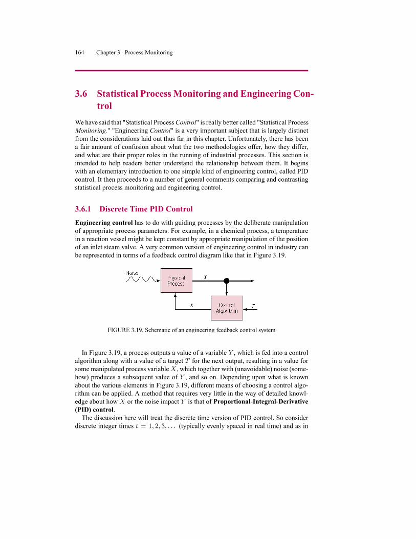
164 Chapter 3. Process Monitoring
3.6 Statistical ProcessMonitoring and Engineering Con-trol
We have said that "Statistical ProcessControl" is really better called "Statistical ProcessMonitoring." "Engineering Control" is a very important subject that is largely distinctfrom the considerations laid out thus far in this chapter. Unfortunately, there has beena fair amount of confusion about what the two methodologies offer, how they differ,and what are their proper roles in the running of industrial processes. This section isintended to help readers better understand the relationship between them. It beginswith an elementary introduction to one simple kind of engineering control, called PIDcontrol. It then proceeds to a number of general comments comparing and contrastingstatistical process monitoring and engineering control.
3.6.1 Discrete Time PID ControlEngineering control has to do with guiding processes by the deliberate manipulationof appropriate process parameters. For example, in a chemical process, a temperaturein a reaction vessel might be kept constant by appropriate manipulation of the positionof an inlet steam valve. A very common version of engineering control in industry canbe represented in terms of a feedback control diagram like that in Figure 3.19.
FIGURE 3.19. Schematic of an engineering feedback control system
In Figure 3.19, a process outputs a value of a variable Y , which is fed into a controlalgorithm along with a value of a target T for the next output, resulting in a value forsome manipulated process variableX , which together with (unavoidable) noise (some-how) produces a subsequent value of Y , and so on. Depending upon what is knownabout the various elements in Figure 3.19, different means of choosing a control algo-rithm can be applied. A method that requires very little in the way of detailed knowl-edge about how X or the noise impact Y is that of Proportional-Integral-Derivative(PID) control.The discussion here will treat the discrete time version of PID control. So consider
discrete integer times t = 1; 2; 3; : : : (typically evenly spaced in real time) and as in

Chapter 3. Process Monitoring 165
Figure 3.19, suppose that
Y (t) = the value of the controlled or output variable at time t ;T (t) = the value of a target for Y at time t, andX(t) = the value of a (manipulated) process variable that is
chosen after observing Y (t) :
A control algorithm converts knowledge of Y (1); Y (2); : : : ; Y (t) and T (s) for all sinto a choice of X(t). For example, in machining Y (t) could be a measured widgetdiameter, T (t) a target diameter, andX(t) a cutting tool position. A control algorithmorders a tool position in light of all past and present diameters and all targets for past,present, and future diameters.The practice of PID control does not typically invest much effort in modeling ex-
actly how changes in X get re�ected in Y . (If the goal of a study was to understandthat relationship, tools of regression analysis might well be helpful.) Nevertheless, inunderstanding the goals of engineering control, it is useful to consider two kinds ofprocess behavior with which engineering control algorithms must sometimes deal.For one thing, some physical processes react to changes in manipulated variables
only gradually. One behavior predicted by many models of physical science is thatwhen initially at "steady state" at time t0, a change of �X in a manipulated variableintroduces a change in the output at time t > t0 of the form
�Y (t) = Y (t)� Y (t0) = G�X�1� exp
��(t� t0)
�
��; (3.51)
for process-dependent constants G and � . Figure 3.20 shows a plot of �Y in display(3.51) as a function of time. In cases where relationship (3.51) holds, G is the limit ofthe ratio �Y=�X and is called the control gain. � governs how quickly the limitingchange in Y is reached (� is the time required to reach a fraction 1� e�1 � :63 of thelimiting change in Y ). It is called the time constant for a system obeying relationship(3.51).
FIGURE 3.20. Change in the output Y (initially at steady state) in response to a �X change inthe manipulated variableX

166 Chapter 3. Process Monitoring
Another phenomenon that is sometimes part of the environment in which engineer-ing control systems must operate is that of dead time or delay between when a changeis made in X and when any effect of the change begins to be seen in Y . If there are �units of dead time and thereafter a relationship similar to that in equation (3.51) holds,one might see a pattern like that shown in Figure 3.21 following an adjustment �Xmade at time t0 on a process at steady state at that time.
FIGURE 3.21. Change in the output Y (initially at steady state) in response to a �X change inthe manipulated variable at time t0 if there are � units of dead time
Of course, not all physical systems involve the kind of gradual impact of processchanges illustrated in Figure 3.20, nor do they necessarily involve dead time. (Forexample, real-time feedback control of machine tools will typically involve changes intool positions that take their full effect "immediately" after being ordered.) But wherethese phenomena are present, they increase the dif�culty of �nding effective controlalgorithms, the dead time problem being particularly troublesome where � is large.To get to the point of introducing the general PID control algorithm, consider a
situation where it is sensible to expect that increasingX will tend to increase Y . De�nethe observed "error" at time t,
Error at Time t E(t) = T (t)� Y (t) ;
and the �rst and second differences of errors
First Differencein Errors atTime t
�E(t) = E(t)� E(t� 1)
and

Chapter 3. Process Monitoring 167
SecondDifference inErrors atTime t
�2E(t) = �(�E(t)) = �E(t)��E(t� 1) :
With some additional algebra
�2E(t) = (E(t)� E(t� 1))� (E(t� 1)� E(t� 2))= E(t)� 2E(t� 1) + E(t� 2) :
Then, for constants �1, �2, and �3, a PID control algorithm sets
PID ControlAlgorithm
�X(t) = �1�E(t) + �2E(t) + �3�2E(t) : (3.52)
(In cases where Y tends to increase with X , the constants �1, �2, and �3 are typicallynonnegative.) The three terms summed on the right of equation (3.52) are respectivelythe proportional, integral, and derivative parts of the control algorithm.
Example 37 PID Control of Final Dry Weight of 20 lb Bond Paper. Through thekind cooperation of the Miami University Paper Science Laboratory and Mr. DougHart, Research Associate at the lab, one of your authors was able to help implement aPID controller on a 13 in Fourdrinier paper-making machine. This machine producespaper in a long continuous sheet beginning with vats of pulp mix. The �nal dry weightof paper is measured as the paper leaves the machine and can be controlled by therate at which a Master�ex peristaltic pump delivers pulp mix to the machine. A manualknob is used to vary the pump speed and can be adjusted in "ticks." (Each 1-tick changecorresponds approximately to a change of pump speed equal to .2% of its maximumcapacity.) Past experience with the machine indicated that for 20 lb bond pulp mixture,a 1-tick increase in pump speed produces approximately a .3 g=m2 increase in paperdry weight. But unavoidable variations in the process (including the "thickness" of themix available to the pump) produce variation in the paper dry weight and need to becompensated for by varying the pump speed.Since there is over a 4min lag between when a pump speed change is made and
when paper affected by the speed change reaches the scanner that measures dry weightat the end of the machine, measurements and corresponding adjustments to pump speedwere made only once every 5min. (This choice eliminates the effect of dead time on thecontrol algorithm, which would be a concern if measurements and adjustments weremade closer together.) Some experimentation with the machine led to the conclusionthat a sensible PID control algorithm for the machine (using the 5-minute intervalsand measuring the control variable changes in terms of ticks) has
�1 = :83; �2 = 1:66; and �3 = :83

168 Chapter 3. Process Monitoring
TABLE 3.9. PID Control Calculations for the Control of Paper Dry Weight (T; Y;E;�E and�2E in g/m2 and�X in ticks)Period, t T (t) Y (t) E(t) �E(t) �2E(t) �X(t) = :83�E(t)
+1:66E(t) + :83�2E(t)1 70:0 65:0 5:02 70:0 67:0 3:0 �2:03 70:0 68:6 1:4 �1:6 :4 1:3284 70:0 68:0 2:0 :6 2:2 5:6445 70:0 67:8 2:2 :2 �:4 3:4866 70:0 69:2 :8 �1:4 �1:6 �1:1627 70:0 70:6 �:6 �1:4 0 �2:1588 70:0 69:5 :5 1:1 2:5 3:8189 70:0 70:3 �:3 �:8 �1:9 �2:73910 70:0 70:7 �:7 �:4 :4 �1:16211 70:0 70:1 �:1 :6 1:0 1:162
in formula (3.52). Table 3.9 shows an actual series of dry weight measurements andPID controller calculations made using these constants. (Since it was impossible tomove the pump speed knob in fractions of a tick, the actual adjustments applied werethose in the table rounded off to the nearest tick.) The production run was begun withthe knob (X) in the standard or default position for the production of 20 lb bond paper.For example, for t = 3,
E(3) = T (3)� Y (3) = 70:0� 68:6 = 1:4;
�E(3) = E(3)� E(2) = 1:4� 3:0 = �1:6;�2E(3) = �E(3)��E(2) = �1:6� (�2:0) = :4;
and so the indicated adjustment (increment) on the pump speed knob is �X(3) =:83�E(3) + 1:66E(3) + :83�2E(3) = :83(�1:6) + 1:66(1:4) + :83(:4) = 1:328ticks. (As actually implemented, this led to a 1-tick increase in the knob position aftermeasurement 3.)
It is useful to separately consider the proportional, integral, and derivative parts ofalgorithm (3.52), beginning with the integral part. With �2 > 0, this part of the algo-rithm increases X when E is positive and thus T > Y . It is this part of a PID controlalgorithm that reacts to (attempts to cancel) deviations from target. Its function is totry to move Y in the direction of T .To grasp why �2E(t) might be called the "integral" part of the control algorithm,
consider a case where both �1 = 0 and �3 = 0 so that one has an "integral only"controller. In this case (supposing that Y (t)'s and T (t)'s with t < 1 are available sothat one can begin using relationship (3.52) at time t = 1), note that
tXs=1
�X(s) = �2
tXs=1
E(s): (3.53)

Chapter 3. Process Monitoring 169
But the sum on the left of equation (3.53) telescopes to X(t)�X(0) so that one has
X(t) = X(0) + �2
tXs=1
E(s):
That is, the value of the manipulated variable is X(0) plus a sum or "integral" of theerror."Integral only" control (especially in the presence of a large time constant and/or
large dead time) often tends to overshoot target values and set up oscillations in thevariable Y . The proportional and derivative parts of a PID algorithm are meant to re-duce overshoot and damp oscillations. Consider next the proportional term from equa-tion (3.52), namely �1�E(t).The proportional part of a PID control algorithm reacts to changes in the error. In
graphical terms, it reacts to a nonzero slope on a plot of E(t) versus t. Where �1 > 0,this part of the algorithm increases X if the error increases and decreases X if Edecreases. In some sense, this part of the algorithm works to hold the error constant(whether at 0 or otherwise).When �1 and �2 have the same sign, the proportional part of a PID control algorithm
augments the integral part when E is moving away from 0 and "brakes" or cancels partof the integral part when E is moving toward 0. Figure 3.22 pictures two plots of Y (t)versus t for cases where the target T is constant. In the �rst plot, Y is approachingT from below. E(t) > 0 while �E(t) < 0. This is a case where the proportionalpart of the algorithm brakes the integral part. In the second plot, Y is above T anddiverging from it. There, both E(t) < 0 and �E(t) < 0, and the proportional part ofthe algorithm augments the integral part. The braking behavior of the proportional partof a PID algorithm helps to resist the kind of oscillation/overshoot problem producedby "integral only" control.
FIGURE 3.22. Two plots of Y against time
To see why �1�E(t) might be called the "proportional" part of the control algo-rithm, consider a case where both �2 = 0 and �3 = 0 so that one has a "proportional

170 Chapter 3. Process Monitoring
only" controller. In this case (supposing that Y (t)'s and T (t)'s with t < 1 are availableso that one can begin using relationship (3.52) at time t = 1),
tXs=1
�X(s) = �1
tXs=1
�E(s): (3.54)
But the sums on both sides of equation (3.54) telescope, so that one has
X(t) = X(0)� �1E(0) + �1E(t):
That is, the value of the manipulated variable is X(0) � �1E(0) plus a term "propor-tional" to the error.Finally, consider the derivative part of the algorithm (3.52), namely �3�2E(t). This
part of the algorithm reacts to curvature or changes in slope on a plot of E (t) versust . That is, it reacts to changes in �E(t). If a plot of errors versus t is linear (�E(t)is constant), this part of the algorithm does nothing to change X . If �3 > 0 and a plotof errors versus t is concave up, the derivative part of algorithm (3.52) will increaseX (and thus Y , decreasing E), while if the plot is concave down it will decrease X .For constant target T , this will tend to "straighten out" a plot of E(t) or Y (t) versus t(presumably then allowing the proportional part of the algorithm to reduce the slope to0 and the integral part to put the process on target). Once again, since "integral only"control often produces unwanted oscillations of Y about a target, and it is impossibleto oscillate without local curvature in a plot of E or Y versus t, the derivative partof the algorithm can be considered as corrective to a de�ciency in the naive "integralonly" idea.The rationale for calling �3�2E(t) the "derivative" part of the PID algorithm (3.52)
is similar to the arguments made about the other two parts. Namely, if �1 and �2 areboth 0 (so that one has "derivative only" control),
tXs=1
�X(s) = �3
tXs=1
�2E(s): (3.55)
Telescoping both sides of equation (3.55) one then has
X(t) = X(0)� �3�E(0) + �3�E(t);and the value of the manipulated variable isX(0)��3�E(0) plus a term proportionalto the change in (or "derivative" of) the error.The primary practical problem associated with the use of PID controllers is the mat-
ter of choosing the constants �1, �2, and �3, sometimes called respectively the propor-tional, integral, and derivative gains for the control algorithm. In simple situationswhere engineers have good mathematical models for the physical system involved,those can sometimes provide at least starting values for searches to �nd good values ofthese constants. Where such models are lacking, various rules of thumb aid searchesfor workable values of �1, �2, and �3. For instance, one such rule is to initially set �1and �3 to zero, increase �2 till oscillations occur, then halve that value of �2 and begin

Chapter 3. Process Monitoring 171
searching over �1 and �3. And it is pretty clear that in systems where a relationshiplike (3.51) holds, the gains �1, �2, and �3 should be inversely proportional to G. Fur-ther, conventional wisdom also says that in systems where there is dead time � > 0,the control gains should decrease (exponentially?) in �. (One should not be changinga manipulated variable wildly if there's to be a long delay before one gets to measurethe impact of those changes and to begin to correct any unfortunate effects one sees.)Ultimately, the matter of �nding good values for the gains �1, �2, and �3 is typ-
ically a problem of empirical optimization. Section 6.2 of this book discusses someexperimental strategies in process optimization. These can be applied to the problemof �nding good constants �1, �2, and �3 in the following way. For given choices of theconstants, one may run the process using the PID controller (3.52) for some number ofperiods, saym. Then a sensible �gure of merit for that particular set of constants is therandom variable
S =1
m
mXt=1
(E(t))2 ;
the average squared error. The empirical optimization strategies of Section 6.2 maythen be applied in an attempt to �nd a set of values for �1, �2, and �3 with minimumassociated mean for S, �s. Chapter problems 38 through 44 describe how the averagesquared error idea was used to arrive at the control algorithm of Example 37.
3.6.2 Comparisons and ContrastsThe PID ideas just discussed are not the only ones used to produce engineering con-trol algorithms. For example, where good models are available for both uncontrolledprocess behavior and for the impact of control actions on process outputs, mathemat-ically optimal control algorithms (that need not be of the PID type) can sometimesbe derived. And the introduction just given completely ignores real issues like themultivariate nature of most industrial applications. (The Y and X just considered areone-dimensional, while real process outputs and possible manipulated variables are of-ten multidimensional.) But the foregoing brief discussion is intended only to give thereader enough of an idea of how engineering control operates to allow the followingcomments on the proper roles of engineering control and statistical process monitoringto make sense.The relative merits of the two methodologies when applied in production contexts
have been at times been hotly debated by their proponents. On some occasions, zealotson one side or the other of the debate have essentially claimed that their methods areuniversally applicable and those of the other side are either without merit or are sim-ply a weak version of their own. The truth is that the methods of statistical processmonitoring and engineering control are not competitors. They are in fact, completelycomplementary, each having its own purposes and appropriate areas of application.When applied to the running of industrial processes, both are aimed at the reductionof unwanted variability. In many applications, they can and should be used togetherin an effort to reduce process variation and improve quality, engineering control help-ing to create stable conditions that are monitored using statistical process monitoring

172 Chapter 3. Process Monitoring
methods.In cases where a process is already physically stable about a target value, statistical
process monitoring tools should only infrequently (and wrongly) signal the need forintervention, and engineering control is of no help in reducing variation. That is, in theclassical stable process situation, tweaking process parameters can only make variationworse, not better. On the other hand, if successive observations on a process look as ifthey are dependent, or if they have means (either constant or moving) different from atarget, engineering control may be able to improve process performance (uniformity ofoutput) essentially by canceling predictable misadjustments of the process. Statisticalprocess monitoring will then protect one from unexpected process changes.Table 3.10 puts side by side a number of pairs of statements that should help the
reader keep clear the basic differences between engineering control and statisticalprocess monitoring as they are applied to industrial processes. The late Dr. Bill Tuckerwas fond of saying "You can't steer a car with statistical process control and you can't�x a car with engineering control." His apt and easily remembered analogy brings intofocus the differences in intent of the two methodologies.
Section 3.6 Exercises1. The target value for a process output variable, Y , is 4 units, and a controllableprocess parameter X is thought to impact Y in a direct fashion. In 3 successiveperiods Y (1) = 2; Y (2) = 1; and Y (3) = 0. You may �nish �lling in a tablelike that below to help you answer this question.Period, t T (t) Y (t) E(t) �E(t) �2E(t) �X(t)
1 22 13 0
(a) What are your values of T (t) here? What is the practical meaning of thisvariable?
(b) What values do you get for E(t);�E(t) and�2E(t) here? Describe whatthese are measuring.
(c) Use control gains �1 = :8; �2 = 1:6; and �3 = 1:9 and compute a PIDcontrol action�X (3) to be taken after observing Y (3).
(d) Howwill this table and future values of Y be used to extend the PID controlof part (c) beyond period 3?
2. In the context of problem 1, suppose that no one is really sure whether Y isaffected by changes in X , or if it is, whether the relationship is "direct" or "in-verse."
(a) Speculate on what might happen if the PID controller of part (c) above isimplemented where Y is completely unrelated to X . What might happenif in fact Y is inversely related to X?

Chapter 3. Process Monitoring 173
TABLE 3.10. Contrasts Between Engineering Control and Statistical Process Control for Indus-trial Processes
Engineering Control Statistical Process Control� In a typical application, there is a sensor on a � This is either manual or automatic plotting
process and an electromechanical adjustment of process performance statistics to warn ofmechanism that responds to orders (for process changes.change of some process parameter) sent by acomputer "brain" based on signals from thesensor.
� This is an adjustment/compensation � This is a detection methodology. Correctivemethodology. Formulas prescribe explicit measures for process changes that arereactions to deviations from target. detected are not speci�ed.
� This is a methodology for ongoing small � There is a tacit assumption here that wiseprocess adjustments. intervention following detection of a process
change will set things perfectly aright (for anextended period).
� There is an explicit expectation of process � There is a tacit assumption here of processinstability/drift in this methodology. stability over long periods.
� This is typically computer (or at least � There is typically a human agent involved inmechanically) controlled. monitoring and interventions.
� The ultimate effect is to keep a process � The ultimate effect is to warn of the presenceoptimally adjusted. of sources of special cause variation, to help
identify them, and to lead to their permanentremoval.
� This is often "tactical" and applied to process � This is often "strategic" and applied to �nalparameters. quality variables.
� In its "optimal stochastic control" version, � This is what one does to monitor for "thethis is what one does within a particular unexpected" (departures from a stableprobability model (for process behavior) to process model of expected behavior).best exploit the probabilistic predictability ofa process.

174 Chapter 3. Process Monitoring
(b) How would you propose to �gure out what, if any, PID control based onXmight be fruitful?
3. In what sense are control charts tools for "controlling" a process? In what mean-ing of the word "control" are they not tools for controlling a process?
3.7 Chapter SummaryShewhart control charts are an engineer's most widely applicable and easily under-stood process-monitoring tools. The �rst four sections of this chapter have introducedthese charts for both variables data and attributes data, considered their use in bothstandards given and retrospective contexts, and discussed their qualitative interpreta-tion and supplementation with sets of "extra alarm rules." Table 3.11 summarizes manyof the standard formulas used in the making of elementary Shewhart charts.
TABLE 3.11. Formulas for Shewhart Control ChartingStandards Given Retrospective
Chart Q �Q �Q UCLQ LCLQ UCLQ LCLQx x � �=
pn �+ 3�=
pn �� 3�=
pn x+A2R x�A2R
x+A3s x�A3sMedian ~x � ��=
pn �+ 3��=
pn �� 3��=
pn
R R d2� d3� D2� D1� D4R D3Rs s c4� c5� B6� B5� B4s B3s
np X nppnp(1� p) np+ 3
pnp(1� p) np� 3
pnp(1� p) (use ppooled for p)
p p pq
p(1�p)n p+ 3
qp(1�p)n p� 3
qp(1�p)n (use ppooled for p)
c X �p� �+ 3
p� �� 3
p� (use �pooled for �)
u u �q
�k �+ 3
q�k �� 3
q�k (use �pooled for �)
The �nal two sections of the chapter have provided context and perspective for thestudy of Shewhart charts and other process-monitoring tools. Section 3.5 introducedthe ARL concept as a means of quantifying the likely performance of a monitoringscheme. Section 3.6 contrasted methods and goals of "engineering control" with thoseof process monitoring when they are both applied in production.
3.8 Chapter 3 Exercises1. What is the purpose of control charting? What is suggested by out-of-controlsignals?

Chapter 3. Process Monitoring 175
2. What makes step 3 in the quality assurance cycle presented in Chapter 1 dif�cultin service contexts? Explain.
3. Why is it essential to have a clear understanding of what constitutes a noncon-formance if a Shewhart c or u chart is to be made?
4. Is control charting most directly concerned with "quality of design" or with"quality of conformance" ?
5. Distinguish between "control limits" and "speci�cation limits" for variables data.
6. Explain the difference between "control limits" and "speci�cation limits" in anattributes data setting.
7. Explain the ARL concept in terms that a person with no statistical training couldunderstand.
8. When designing a control chart, what kinds of ARL values are desirable foran on-target process? For an off-target process? Explain why your answers arecorrect from an economic point of view.
9. State why statistical methodology is an unavoidable part of quality assurancepractice. (Review Chapter 1.)
10. Sometimes the plotted statistics appearing on a Shewhart control chart hug (orhave little scatter around) a center line. Explain why this is not necessarily agood sign.
11. Uninformed engineers sometimes draw in lines on Shewhart x charts at engi-neering speci�cations for individual measurements. Why is that bad practice?
12. It is common to hear people imply that the job of control charts is to warn ofdegradation in product quality. Do you agree with that? Why or why not?
13. What is the purpose of sets of "extra alarm rules" like the Western Electric rulespresented in Section 3.4?
14. What (relevant to quality improvement efforts) does a multimodal shape of ahistogram for a part dimension suggest? (Review Chapter 2.)
15. In colloquial terms, the language "control" chart perhaps suggests a plot associ-ated with continuous regulatory efforts. Is understanding correct? Why or whynot? Suggest a better term than "control chart."
16. Journal Diameters. Below are some summary statistics (means and standarddeviations) for journal diameters of tractor axles as the axles come off an au-tomatic grinding machine. The statistics are based on subgroups of size n = 4pieces taken once per hour. The values listed are in millimeters. Speci�cationson the journal diameter are from 44:975mm to 44:990mm.

176 Chapter 3. Process Monitoring
Subgroup x s Subgroup x s1 44:9875 :0029 11 44:9815 :00172 44:9813 :0025 12 44:9815 :00173 44:9808 :0030 13 44:9810 :00244 44:9750 :0000 14 44:9778 :00215 44:9783 :0039 15 44:9748 :00246 44:9795 :0033 16 44:9725 :00297 44:9828 :0021 17 44:9778 :00218 44:9820 :0024 18 44:9790 :00349 44:9770 :0024 19 44:9785 :001010 44:9795 :0010 20 44:9795 :0010
Note thatPx = 899:5876 and
Ps = :0442.
(a) Are the above attributes data or variables data? Why?
(b) Make a retrospective s chart for these values.
(c) Make a retrospective x chart for these values.
(d) What do these charts indicate (in retrospect) about the stability of the grind-ing process?
(e) Based on your conclusion in (d), can the fraction of journal diameters thatcurrently meet speci�cations be reliably estimated? Why or why not?
(f) Independent of your conclusion in (d), if one judged the process to be sta-ble based on the 20 subgroups summarized above, what could be used asan estimate of the fraction of journal diameters that currently meet spec-i�cations? (Give a number based on a normal distribution assumption fordiameter measurements.)
(g) Suppose that henceforth (into the future) this process is to be monitoredusing subgroups of size n = 5. Give control limits for a (standards given)median chart based on the mid-speci�cation (giving the center line) andyour estimated process standard deviation from (b).
(h) Give control limits for future monitoring of sample ranges (use your esti-mated process standard deviation from (b) as a future standard value andassume n = 5).
17. Refer to the Journal Diameter case introduced in problem 16. Sometimes sub-group size is not constant. When using standard deviations from subgroups ofvarying sizes n1; n2; :::; nr to estimate �, there are several possibilities. Of com-monly used ones, the one with the best theoretical properties is
spooled =
s(n1 � 1)s21 + (n2 � 1)s22 + � � �+ (nr � 1)s2r(n1 � 1) + (n2 � 1) + � � �+ (nr � 1)
:

Chapter 3. Process Monitoring 177
Another possibility is
� =
(n1 � 1)s1c4(n1)
+(n2 � 1)s2c4(n2)
+ � � �+ (nr � 1)src4(nr)
n1 + n2 + � � �+ nr � r:
(Since sample sizes vary in this development, we are displaying the dependenceof c4 on sample size here.) The most appropriate estimator of a common mean,�, when sample sizes vary is
xpooled =n1x1 + n2x2 + � � �+ nrxr
n1 + n2 + � � �+ nr:
Consider the subgroup means and standard deviations given in problem 16. Sup-pose subgroups were of size n = 4 except for the ones indicated in the followingtable.Subgroup Sample Size
1 28 210 815 518 319 320 9
(a) Find values for spooled, �, and xpooled.(b) Give two estimates of 1) the standard deviation of a subgroup mean when
n = 2 and 2) the standard deviation of a subgroup standard deviation whenn = 2. (Hint: Varxi = �2=ni and Var si = �2(1� c24(ni)).)
(c) With the new subgroup sizes, consider two retrospective control charts, onechart appropriate for assessing the constancy of variability of axle jour-nal diameters and the other for monitoring average axle journal diameter.Would the control limits be constant across time for the two charts? (Thereis no need to actually make them here.) Why or why not? (See (a) and (b).)
(d) Do the center lines for the two charts in (c) change depending on subgroupsize? (Again, there is no need to make the charts.) Why or why not?
18. Rolled Paper. Shervheim and Snider did a project with a company that cutsrolled paper into sheets. The students periodically sampled n = 5 consecutivesheets as they were cut and recorded their actual lengths, y. Data from 20 sub-groups are summarized below. (Measurements corresponding to the values in thetable were in 64ths of an inch above nominal, i.e., x = y � nominal.)
(a) Make a retrospective s chart.(b) Make a retrospective x chart.

178 Chapter 3. Process Monitoring
(c) What do these charts indicate (in retrospect) about the stability of the cut-ting process?
(d) Give an estimate of the process standard deviation based on s.(e) If one judges the process to be stable and sheet length to be normally dis-
tributed, estimate the fraction of sheets below nominal in length. (Hint:Find P (x < 0) by transforming to a standard normal random variable Z.)
Subgroup x s1 12:2 :842 11:2 1:643 10:6 2:074 12:2 2:495 11:2 :846 12:6 1:827 12:2 2:958 13:6 1:679 12:2 1:3010 10:4 1:5211 10:4 1:9512 10:6 1:6713 10:4 1:6714 12:0 2:9115 11:2 :8416 10:6 1:8217 10:4 1:1418 9:8 2:1719 9:6 2:0720 10:6 1:95
224:0 35:33
(f) Each :25 in that the cutting process mean is above nominal represents a$100,000/year loss to the company from product "given away." On theother hand, the company wants to be sure that essentially no sheets areproduced with below-nominal lengths (so they want �x > 3�). With thisin mind, what adjustment in mean length do you suggest, and what yearlysavings or additional cost do you project if this adjustment is made?
(g) Suppose that the adjustment you recommend in (f) is made and henceforththe cutting process is to be monitored based on samples of size n = 3.What are standards given control limits for future monitoring of x and s?
(h) Suppose that while using your x chart from (g) the process mean suddenlydrops to the point where 1% of the sheets produced are below nominalin length. On average, how many samples will be required to detect this?(Hint: �nd the "new �x" that will make P (x < 0) = :01, then using it�nd P (x < LCL) + P (x > UCL):) How does this compare in terms of

Chapter 3. Process Monitoring 179
quickness of detection to a scheme (essentially a p chart) that signals the�rst time a sample of n = 3 contains at least one sheet with below-nominallength?
19. Refer to theRolled Paper case in problem 18. Again use the means and standarddeviations given there, but suppose that the number of sheets per subgroup wasnot constant. Instead, suppose subgroups contained 5 sheets except for the onesindicated in the following table.Subgroup Subgroup Size
3 76 710 214 417 319 220 6
(a) Compute xpooled and two different estimates of �. (See problem 17.)(b) For a subgroup size of n = 7, give two estimates of 1) the standard de-
viation of a subgroup mean and 2) the standard deviation of a subgroupstandard deviation. (Hint: Varxi = �2=ni and Var si = �2(1� c24(ni)).)
(c) With the variable subgroup sizes, consider two retrospective control charts,one s chart and one x chart. Would the control limits be constant acrosstime for either chart? (There is need to make the charts.) Why or why not?(See (a) and (b).)
(d) Do the center lines for the two charts in (c) remain across subgroup sizes?(Again, there is no need to make the charts.) Why or why not?
20. U-bolt Threads. A manufacturer of U-bolts for the auto industry measures andrecords thread lengths on bolts that it produces. Eighteen subgroups, each of n =5 consecutive bolts, were obtained and actual thread lengths y were measured.These can be expressed as deviations from nominal by transforming x = y �nominal. Some summary statistics are indicated below (the units are :001 inabove nominal).
(a) Estimate the supposedly common subgroup standard deviation, �, using 1)the subgroup ranges (Ri) and 2) the subgroup standard deviations (si).
(b) Find control limits for the subgroup ranges. (Use the estimate of � basedon the si.)
(c) Find control limits for the subgroup standard deviations. (Use the estimateof � based on the si.)
(d) Plot the ranges and standard deviations on Shewhart charts using the ret-rospective limits from (b) and (c). Is it plausible that variability of thread

180 Chapter 3. Process Monitoring
length was constant from sampling period to sampling period?Why or whynot?
(e) Find retrospective control limits for the subgroup means. (Use your esti-mate of � based on the si.) Plot the means on a Shewhart chart with theselimits.
Subgroup Thread Length ~x s x R1 11; 14; 14; 10; 8 11 2:61 11:4 62 14; 10; 11; 10; 11 11 1:64 11:2 43 8; 13; 14; 13; 10 13 2:51 11:6 64 11; 8; 13; 11; 13 11 2:05 11:2 55 13; 10; 11; 11; 11 11 1:10 11:2 36 11; 10; 10; 11; 13 11 1:22 11:0 37 8; 6; 11; 11; 11 11 2:30 9:4 58 10; 11; 10; 14; 10 10 1:73 11:0 49 11; 8; 11; 8; 10 10 1:52 9:6 310 6; 6; 11; 13; 11 11 3:21 9:4 711 11; 14; 13; 8; 11 11 2:30 11:4 612 8; 11; 10; 11; 14 11 2:17 10:8 613 11; 11; 13; 8; 13 11 2:05 11:2 514 11; 8; 11; 11; 11 11 1:34 10:4 315 11; 11; 13; 11; 11 11 :89 11:4 216 14; 13; 13; 13; 14 13 :55 13:4 117 14; 13; 14; 13; 11 13 1:22 13:0 318 13; 11; 11; 11; 13 11 1:10 11:8 2
202 31:51 200:4 74
(f) Setting the center line at x, �nd upper and lower control limits for the sub-group medians. (Use your estimate of � based on the si.) Plot the medianson a Shewhart chart with these limits.
(g) What do the charts in (e) and (f) suggest about the threading process?(h) A U-bolt customer requires that essentially all U-bolt thread lengths are
within :011 in of nominal. Assuming bolt manufacturing continues as rep-resented by the values in the table, will the customer be satis�ed with cur-rent production? Why or why not? Give a quantitative defense of your an-swer assuming normality of thread length. (Hint: Find P (�11 < x < 11).)
21. Refer to the U-bolt Threads case in problem 20. Problem 17 presented ways ofestimating � when r subgroups are of varying size ni. The formulas there arebased on subgroup sample standard deviations si. Another expression sometimesused to estimate the process standard deviation is based on ranges, namely
(n1 � 1)R1d2(n1)
+(n2 � 1)R2d2(n2)
+ � � �+ (nr � 1)Rrd2(nr)
n1 + n2 + � � �+ nr � r:

Chapter 3. Process Monitoring 181
Consider the subgroup means and ranges given in problem 20 and suppose thatsubgroups consisted of n = 5 bolts except for the subgroups indicated in thefollowing table:Subgroup Subgroup Size
2 85 46 67 211 314 715 218 2
(a) Give xpooled and three estimates of �. Base two of the estimates of � onthe subgroup standard deviations and the other on the ranges.
(b) Find three estimates of the standard deviation of a subgroup mean whenn = 8. Base two of the estimates on subgroup standard deviations and oneon the ranges. (Hint: Varxi = �2=ni.)
(c) Find three estimates of the standard deviation of each subgroup samplestandard deviation when n = 8. Base two of the estimates on subgroupstandard deviations and one on the ranges. (Hint:Var si = �2(1�c24(ni)).)
(d) Find an estimate of the standard deviation of each subgroup range whenn = 8. Base the estimate on the subgroup ranges. (Hint:VarRi = d23(ni)�2.)
(e) Consider retrospective x and R charts using the new con�guration of sub-group sizes. (There is no need to make the charts here.) Would controllimits for either chart be constant across time? Why or why not?
(f) Are the center lines for the charts referred to in (e) constant across sub-groups? Why or why not?
22. Turning. Allan, Robbins, and Wycoff worked with a machine shop that employsa CNC (computer numerically controlled) lathe in the machining of a part for aheavy equipment manufacturer. Some summary statistics for a particular partdiameter (x) obtained from 25 subgroups of n = 4 parts turned on the lathe aregiven below. The units are inches.
(a) Find retrospective control limits for the values (both means and ranges).What do the x and R values indicate about the stability of the turningprocess?
(b) Suppose that one wishes to apply the four Western Electric alarm rules tothe x values. Specify the different zones to be used for the mean diame-ters. Are any of the rules violated in the �rst 10 samples? (If you �nd anyviolations, say which rule is violated for the �rst time where.)

182 Chapter 3. Process Monitoring
Subgroup x R1 1:18093 :00012 1:18085 :00023 1:18095 :00024 1:18063 :00085 1:18053 :00076 1:18053 :00057 1:18058 :00058 1:18195 :00019 1:18100 :000310 1:18095 :000111 1:18095 :000612 1:18098 :000113 1:18123 :000914 1:18128 :000215 1:18145 :000716 1:18080 :000317 1:18100 :000018 1:18103 :000119 1:18088 :000320 1:18100 :000021 1:18108 :000222 1:18120 :000423 1:18088 :000224 1:18055 :002225 1:18100 :0004
29:52421 :0101
(c) Give an estimate of the process short-term standard deviation derived fromthe ranges (use all 25 subgroups) and the assumption that � is constant overthe study period.
(d) Engineering speci�cations on the diameter in question were in fact 1:1809� :005 in.Suppose that over short production runs, diameters can be described asnormally distributed and that your estimate of � from (c) is an appropriatedescription of the variation seen in short runs. Give an estimate of the bestpossible fraction of diameters meeting speci�cations available using thisparticular lathe.
(e) Make further use of your estimate of � from (c), and set up control limitsthat could be used in the future monitoring of the process standard devia-tion via Shewhart charting of s based on samples of size n = 5.
(f) Again use your estimate of � from (c) and consider future monitoring of xbased on samples of size n = 4 using "3 sigma" limits and a center line atthe target diameter, 1:1809. Assuming diameters are normally distributed,

Chapter 3. Process Monitoring 183
on average how many subgroups would be required to detect a change inmean diameter, �, from 1:1809 to 1:1810?
23. Refer to the Turning case in problem 22. Problem 21 presented a method forestimating � based on ranges of subgroups of varying size. Use that method inthis problem. Use again the subgroup means and ranges given in problem 22 andsuppose all subgroups were of size n = 4 parts except for the ones indicated inthe following table.Subgroup Subgroup Size
1 24 35 69 211 713 515 316 217 818 2
(a) Give xpooled and an estimate of �.(b) Find an estimate of the standard deviation for a subgroup mean, xi, when
n = 7.(c) Find an estimate of the standard deviation for a subgroup range, Ri, when
n = 7.(d) Consider retrospective x and R charts using the new con�guration of sub-
group sizes. (There is no need to make the chart here.) Are the controllimits for the two charts constant across subgroups? Why or why not?
(e) Are the center lines for the charts considered in (d) constant across sub-groups? Why or why not?
24. Package Sorting. Budworth, Heimbuch, and Kennedy analyzed a company'spackage sorting system. As packages arrive at the sorting system, they are placedonto trays and the bar codes af�xed to the packages are scanned (in an operationmuch like the scanning process at a grocery store checkout). Bar code identi�-cation numbers begin with the zip code of the package destination. This permitspackages to be sorted into 40 bins, each of which represents a different bulkmail center (BMC) or auxiliary service facility (ASF). All packages in a givenbin are shipped by truck to the same mail center. The bulk transportation of thesepackages is much cheaper than if they were mailed directly by the nearest U.S.Post Of�ce. The large number of BMC packages handled daily by the companyproduces tremendous cost savings.Initially, the team tackled the so-called "no chute open" problem. When one ofthe BMC bins is full and packages destined for that bin cannot be dropped into

184 Chapter 3. Process Monitoring
it. They end up in a "no chute open" bin. This eventuality produced many inef-�ciencies and even shutdowns of the entire system. In fact, the system was shutdown about 10min=day on average because of this problem. This lost time costthe company the ability to process about 400 packages/day, and accumulatedover a year, this represents a serious loss. The team decided to document thenumber of packages per shift dumped in the "no chute open" bin. The data theycollected are below.
Number in"No Chute
Date Shift Open" Bin10/16 1 151010/17 3 62210/18 1 213210/18 2 154910/19 1 120310/19 2 275210/19 3 153110/20 1 131410/20 2 206110/20 3 98110/21 1 163610/21 2 255910/21 3 121210/22 1 201610/22 2 276510/22 3 574
(a) Is this an attributes data problem or a variables data problem? Why?(b) What constitutes a "subgroup" in the context of this problem?(c) What probability model is a possible description of the number of packages
routed to the "no chute open" bin during a given shift?(d) Assuming the sorting process is stable, estimate the average number of
packages routed to the "no chute open" bin during a particular shift. Esti-mate the standard deviation of the number of packages routed to the "nochute open" bin. These estimates should be consistent with your answer to(c).
(e) Was the number of packages in the "no chute open" bin apparently constantexcept for random �uctuation?Why or why not? Defend your answer usinga control chart.
25. Refer to the Package Sorting case in problem 24. Budworth, Heimbuch, andKennedy were told that the sorting system was set up to let a package circle onthe conveyor belt for 10 cycles (once each cycle the package would fall into thecorrect chute if that chute was not occupied). If after 10 cycles the correct chute

Chapter 3. Process Monitoring 185
was always occupied, a package would be consigned to the inef�cient "no chuteopen" bin. Upon observing the system in operation, the team immediately recog-nized packages dropping into the "no chute open" bin after only 2 or 3 cycles.Management was noti�ed and the programming of the system was corrected.The team gathered the data below after the correction.
Number in"No Chute
Date Shift Open "Bin10/23 1 12410/24 3 55010/25 1 010/25 2 6810/25 3 54310/26 1 38310/26 2 8210/26 3 118
(a) Extend the control limits from your chart in part (e) of problem 24. Plotthe data above on the same chart. Does it appear the system change waseffective? Why or why not?
(b) Make a chart to assess stability of the number of packages in the "no chuteopen" bin using only the data above. Does it appear the system was stable?Why or why not?
(c) Has the team solved the problem of a large number of packages in the "nochute open" bin? Defend your answer.
26. Refer to the Package Sorting case of problems 24 and 25. Budworth, Heimbuch,and Kennedy also investigated the performance of the package scanning equip-ment. Just as items at a cashier's scanner often are not read on the �rst scan, sotoo were bar codes on packages not necessarily read on the �rst or second scan.Label damage and incorrect orientation, erroneous codes, and some simply un-explained failures all produced "no read" packages. If a package was not read onthe �rst pass, it continued on the carousel until reaching a second scanner at theend of the carousel. Failure to read at this second scanner resulted in the packagebeing dropped into a "no read" bin and scanned manually with a substantial lossin ef�ciency. The team took data over 30 consecutive one-minute periods on thevariables
n = the number of packages entering the system during the 1min period ,X1 = the number of those packages failing the �rst scan, andX2 = the number of those packages failing both scans .
The values they recorded follow.

186 Chapter 3. Process Monitoring
Minute n X1 X2 Minute n X1 X21 54 10 2 16 66 17 02 10 3 2 17 56 11 33 55 22 3 18 26 6 14 60 18 5 19 30 6 05 60 12 1 20 69 14 16 60 14 1 21 58 23 57 37 14 0 22 51 18 58 42 17 1 23 32 15 19 38 20 10 24 44 23 410 33 6 2 25 39 13 211 24 6 3 26 26 3 112 26 7 5 27 41 17 113 36 12 0 28 51 25 514 32 10 3 29 46 18 115 83 25 2 30 59 23 6
(a) What constitutes a "subgroup" in this problem?(b) Is this an attributes data or a variables data problem? Why?(c) Make a retrospective control chart to assess consistency of the proportion
of packages failing both scans and comment on what it indicates.(d) Make a retrospective control chart to assess consistency of the proportion
of packages that are not read on the �rst scan and comment on what itindicates.
(e) Make a retrospective control chart to assess consistency of the proportionof all packages in a given minute that are not read on the �rst scan and areread on the second scan. Comment on what it indicates.
(f) Calculate the proportions of those packages failing the �rst scan that alsofail the second scan.
(g) Make a retrospective control chart to assess consistency of the proportionsin (f). Comment on what it indicates.
27. Jet Engine Visual Inspection. The data below are representative of counts ofnonconformances observed at �nal assembly at an aircraft engine company. Sup-pose that one �nal assembly is inspected per day.
(a) Is this a variables data problem or is it an attributes data problem? Explain.(b) In the context of the problem, what is a "subgroup"?(c) What probability distribution is a likely model for counts of nonconfor-
mances on these engines? Defend your answer.(d) Find an estimated mean number of visually identi�ed nonconformances
and the corresponding estimated standard deviation.

Chapter 3. Process Monitoring 187
Number of Number of Number ofDay Nonconformances Day Nonconformances Day Nonconformances7/5 15 7/15 18 7/29 167/6 19 7/16 4 8/1 307/7 12 7/19 16 8/2 347/8 24 7/20 24 8/3 307/9 18 7/21 16 8/4 407/10 10 7/22 12 8/5 307/11 16 7/25 0 8/6 367/12 26 7/26 16 8/8 327/13 16 7/27 26 8/9 427/14 12 7/28 12 8/10 34
(e) Find appropriate upper and lower control limits and center line to applyto the counts. Make the corresponding control chart for these data. Doesit appear that the process was stable over the period of the study? Why orwhy not? Identify any out-of-control points. Apply Nelson's rules.
(f) Suppose two inspectors were involved in the data collection. Brie�y dis-cuss what must be true (in terms of data collection protocol) to assure thatthe chart and analysis in (e) are credible.
28. Refer to the Jet Engine Visual Inspection case in problem 27.
(a) When possible causes for out-of-control points on a control chart are ad-dressed and physically eliminated, it is common practice to discard the dataassociated with those out-of-control points and recalculate control limits.Apply this thinking to part (e) of problem 27, assuming causes of the out-of-control points have been addressed (you should "throw out" July 16, 25and August 1 through 10�a total of 11 out of 30 points).
(b) Suppose the following data are obtained in visual inspection of �nal engineassemblies over the next three days.
Assemblies Number ofDay Inspected Nonconformances1 :5 82 2:0 313 1:5 26
(Partial inspection of �nal engine assemblies could possibly occur becauseof unforeseen labor problems. More than one engine assembly might beinspected on days 2 and 3 to, in some sense, make up for the partial inspec-tion on day 1.) Using the information from (a) above, �nd control limitsfor nonconformance rates on these three days (don't use the number ofnonconformances during these 3 new days to �nd the limits). Also give thecenter line and three plotted values (nonconformances per engine assemblyinspected).
(c) Do your values from part (b) suggest process instability? Explain.

188 Chapter 3. Process Monitoring
(d) Your center line should be constant across the three days represented in (b).Why is this?
29. The number of standard units inspected may vary from period to period. Let
Xi = the number of nonconformances observed at period i,ki = the number of standard units inspected at period i, andui = Xi=ki :
The following values were obtained over 9 periods.
i 1 2 3 4 5 6 7 8 9ki 1 2 1 3 2 1 1 3 1ui 0 3:00 0 1:33 4:00 0 0 :67 1:00
(a) From these values, what conclusions can you make about stability of theprocess being monitored? Make the appropriate control chart.
(b) Suppose that in the future ki will be held constant at 1 and that 2:4 noncon-formances per inspection unit will be considered to be "standard quality."Find the probability of an out-of-control signal on a 3-sigma Shewhart con-trol chart, if the true nonconformance rate is at the standard quality level(� = 2:4). Find the probability of an out-of-control signal if the true non-conformance rate changes to � = 4:8. (Remember that the Poisson(�)probability function is P (X = x) = (exp (��)�x) =x! .)
(c) Suppose that in the future ki will be held constant at 2. Find the probabilityof an out-of-control signal if the true nonconformance rate is at the standardquality level (� = 2:4). Find the probability of an out-of-control signal ifthe true nonconformance rate changes to � = 4:8
(d) Compare your answers to (b) and (c). Which subgroup size (k = 1 ork = 2) is more appealing? Why?
30. Electrical Switches. The following scenario is taken from an aircraft enginecompany's training material. One hundred electrical switches are sampled fromeach of 25 consecutive lots. Each sampled switch is tested and the sample num-bers failing are recorded below.
(a) Find the sample fractions of switches failing the test.
(b) What is a plausible probability model for describing the count of switchesin a particular sample failing the test? Explain.
(c) Plot the number failing versus the sample period. Plot an appropriate centerline and control limits on the same graph.
(d) What does your plot in (c) monitor here?

Chapter 3. Process Monitoring 189
(e) Interpret your plot in (c). Identify any out-of-control points.
Sample Number Failing Sample Number Failing1 11 14 182 9 15 73 15 16 104 11 17 85 22 18 116 14 19 147 7 20 218 10 21 169 6 22 410 2 23 1111 11 24 812 6 25 913 9
(f) What is the usual name of the chart you prepared in part (c)?
(g) Suppose causes for out-of-control points identi�ed in (e) are identi�ed andphysically removed. It would then make sense to delete the out-of-controlpoints and recalculate limits. Do this recalculation and redo (c). You shouldhave identi�ed and eliminated 2 out-of-control points.
(h) Suppose the number of switches sampled and the number failing for thenext three consecutive lots are as follows.Number Sampled Number Failing
75 8144 1290 11
Using your estimated fraction failing from (g) as a standard for judgingthese samples, �nd control limits and center lines appropriate for the threenew "number failing" data points. Are the three sets of control limits andcenter lines the same? Why is this to be expected?
31. A data set in the book Elementary Statistical Quality Control by Burr indicatesthat in the magna�ux inspection for cracks in a type of malleable casting, aboutp � :11 of the castings will have detectable cracks. Consider the examination of12 such castings. Let X be the number of castings from the set of 12 identi�edas being cracked.
(a) Find P [X = 5].
(b) Find P [X > 5].
(c) Find EX .
(d) Find Var X .

190 Chapter 3. Process Monitoring
(e) Ten sets of 12 castings are to be inspected. What is the probability that atleast one set of 12 will have one or more cracked castings?
32. Plastic Packaging. This is a plastic packaging case investigated by Hsiao, Linseand McKay. Plastic bags were supposed to hold three bagels each. An ideal bagis 6:75 in wide, has a 1:5 in lip, and has a total length of 12:5 in (including thelip). The ideal hole positions are on the lip. The hole position on selected bagswas measured as the distance from the bottom of the bag to the hole. Five bagswere obtained at six times on each of three days. Hole position, bag width, baglength, and lip width were measured and recorded for each bag. The data forhole position (in inches) are below.
Day Time Hole Position1 10:10 am 1:87500; 1:84375; 1:87500; 1:84375; 1:843751 10:25 am 1:90625; 1:90625; 1:90625; 1:87500; 1:906251 10:55 am 1:87500; 1:93750; 1:93750; 1:93750; 1:968751 11:12 am 2:09375; 2:12500; 2:21875; 2:15625; 2:125001 11:35 am 2:00000; 2:00000; 2:00000; 2:00000; 2:031251 11:41 am 1:87500; 1:90625; 1:90625; 1:87500; 1:937502 8:15 am 1:62500; 1:62500; 1:59375; 1:65625; 1:593752 8:54 am 1:62500; 1:62500; 1:59375; 1:68750; 1:656252 9:21 am 1:62500; 1:59375; 1:62500; 1:59375; 1:625002 9:27 am 1:62500; 1:59375; 1:62500; 1:65625; 1:656252 9:51 am 1:56250; 1:59375; 1:56250; 1:56250; 1:562502 9:58 am 1:56250; 1:56250; 1:56250; 1:53125; 1:562503 10:18 am 1:50000; 1:56250; 1:53125; 1:53125; 1:500003 10:33 am 1:53125; 1:53125; 1:53125; 1:53125; 1:500003 10:45 am 1:50000; 1:53125; 1:50000; 1:53125; 1:468753 11:16 am 1:50000; 1:50000; 1:50000; 1:53125; 1:500003 11:24 am 1:53125; 1:53125; 1:50000; 1:50000; 1:500003 11:39 am 1:50000; 1:50000; 1:53125; 1:53125; 1:53125
(a) What is a natural subgroup in this situation?
(b) How many items are in each subgroup described in (a)? How many sub-groups are there here in total?
(c) Calculate the subgroup means and subgroup ranges.
(d) Make a retrospective control chart for mean hole position. Give the centerline, control limits, and zone limits.
(e) Make a retrospective control chart for variability in position using yourvalues from (c). Give the control limits and zone limits.
(f) What is the usual name of the chart in (d)? What is the usual name of thechart in (e)?

Chapter 3. Process Monitoring 191
(g) Is it important which of the charts developed in (d) and (e) is analyzed �rst?Why or why not?
(h) Find the estimated standard deviation of hole position based on the ranges.
33. Refer to the Plastic Packaging case in problem 32.
(a) Calculate the 18 subgroup means and 18 subgroup ranges.
(b) For each day separately, make retrospective control charts for mean holeposition. Give center lines, control limits, and zone limits. What do thesecharts suggest about process performance?
(c) For each day separately, make retrospective control charts for variability ofhole position.
(d) Based on your answer to (c), is variability of hole location constant withinany one of the days? Why or why not?
(e) According to your charts in (c), is there a day in which a single standarddeviation of hole position is plausible? Why or why not?
(f) Suppose your answer in (e) is "yes" for each day. Find estimated �'s forthe three different days treated separately. (Base your estimates on sampleranges.)
(g) Comment on how your estimates in (f) compare to the estimate in part (h)of problem 32.
34. Refer to the Plastic Packaging case in problems 32 and 33. The ideal lip widthis 1:5 in. The lip width data below (in inches) were taken on the same bagsrepresented in problem 32.
(a) Is this a variables data or an attributes data scenario? Why?
(b) Find the subgroup means, ranges, and standard deviations.
(c) Make retrospective control charts for lip width variability and lip widthmean based on the sample ranges.
(d) In view of the appearance of your chart for variability of lip width, doesit make sense to seriously examine the chart for mean lip width? Why orwhy not?
(e) Instead of making the completely retrospective charts asked for in (c), is itpossible to incorporate some "standards" information and make a differentchart for mean lip width? Explain.
(f) Instead of treating all 18 samples at once as in part (c), for each day sep-arately, make retrospective R and x charts. What are your conclusionsregarding process stability for each day separately?

192 Chapter 3. Process Monitoring
Day Time Lip Width1 10:10 am 1:75000; 1:62500; 1:62500; 1:65625; 1:625001 10:25 am 1:62500; 1:62500; 1:62500; 1:65625; 1:656251 10:55 am 1:53125; 1:53125; 1:50000; 1:50000; 1:500001 11:12 am 1:40625; 1:43750; 1:43750; 1:46875; 1:468751 11:35 am 1:46875; 1:46875; 1:46875; 1:46875; 1:406251 11:41 am 1:43750; 1:43750; 1:46875; 1:50000; 1:468752 8:15 am 1:37500; 1:40625; 1:37500; 1:40625; 1:375002 8:54 am 1:37500; 1:43750; 1:43750; 1:40625; 1:406252 9:21 am 1:40625; 1:37500; 1:43750; 1:40625; 1:406252 9:27 am 1:50000; 1:46875; 1:43750; 1:46875; 1:437502 9:51 am 1:43750; 1:43750; 1:43750; 1:43750; 1:437502 9:58 am 1:53125; 1:46875; 1:53125; 1:50000; 1:531253 10:18 am 1:53125; 1:56250; 1:50000; 1:50000; 1:531253 10:33 am 1:50000; 1:53125; 1:53125; 1:50000; 1:500003 10:45 am 1:34375; 1:34375; 1:34375; 1:37500; 1:375003 11:16 am 1:46875; 1:46875; 1:46875; 1:43750; 1:437503 11:24 am 1:37500; 1:40625; 1:40625; 1:40625; 1:406253 11:39 am 1:43750; 1:43750; 1:40625; 1:37500; 1:43750
(g) Find three daily estimated lip width standard deviations. How do theseestimates compare to that calculated when the complete set of data is used?(See (c) above.)
(h) Would there be advantages to using subgroup standard deviations insteadof subgroup ranges in parts (c) and (f) above? Explain.
35. Refer to the Plastic Packaging case in problem 32.
(a) Make a control chart for the standard deviation of hole position. Is shortterm variation stable?
(b) Make a control chart for mean hole position based on subgroup standarddeviations. Is process aim stable?
(c) For each day separately, make charts for the standard deviation of holeposition. Is short term variation stable for each day?
(d) For each day separately, make charts for mean hole position (use an esti-mate of � based on the subgroup standard deviations). Is process aim stablefor each day?
(e) For each of (a), (b), (c), and (d), was it helpful to use the subgroup standarddeviations instead of the subgroup ranges as in problem 32? Why or whynot?
36. Refer to the Hose Skiving case of problem 11 in the Chapter 1 exercises. Theplant works two shifts/day. Five hoses were sampled every two hours from each

Chapter 3. Process Monitoring 193
of three production lines and skive length, y measured. Speci�cations for skivelength are target � :032 inches. The values (x = y � target) in the accompa-nying tables are in units of :001 in above target.
(a) Explain (possibly using the notions of "rational subgrouping" and "strat-i�cation") why it would not make good sense to combine data taken at aparticular time period from the three different production lines to make asingle "sample." (Particularly in cases where it is only possible to select asingle item from each line at a given time period, the urge to make such a"sample" is strong, and this kind of error is a common one.)
(b) Compute the 48 sample means and ranges for the data given here Thenseparately for lines 1, 2, and 3 make an x chart and an R chart. Commenton what they indicate about the stability of the skiving process on the threelines over the two days of this study.
(c) One could think about plotting all 48 sample means on a single chart, forexample plotting means from lines 1, 2, and 3 in that order at a given timeperiod. Discuss why that is not a terribly helpful way of summarizing thedata. (Will it be easier or harder to see trends for a given production line onthis kind of plot or on the separate charts of part (b)?)
Day Time1 8:00 am1 10:00 am1 12:00 pm1 2:00 pm1 4:00 pm1 6:00 pm1 8:00 pm1 10:00 pm2 8:00 am2 10:00 am2 12:00 pm2 2:00 pm2 4:00 pm2 6:00 pm2 8:00 pm2 10:00 pm
Line 1Skive Length
3; 2; 4;�5; 25;�4;�3; 0;�2�5; 5; 5;�3; 2�2; 5; 4;�3; 2�10; 2; 1; 2; 1
�5;�6;�3;�3;�7�5; 0;�3;�3;�8
�5;�10; 10;�9;�32; 4; 1; 0;�5
�3; 3;�4; 5; 3�5;�7; 6; 8;�103;�4; 4; 6;�3
�10;�7;�3;�1;�30;�1;�6;�2; 02; 4;�2;�3; 51; 0;�1; 7;�5
Line 2Skive Length�17; 3; 2; 10; 413; 3;�2; 12; 1514; 6; 10; 5; 17; 2; 10; 16; 13
�15;�12;�2;�4; 0�4;�6;�4;�4; 42;�5;�5;�3;�40;�1;�2;�1; 015; 2; 16; 10; 14
12; 4;�10; 10;�31;�7; 4;�5;�9�6; 8;�5; 18; 20
�2;�4;�5;�1;�3�2;�2;�2;�4;�2
0; 2;�1;�1;�2�1;�2; 0;�1;�1
Line 3Skive Length�3;�5; 7; 10; 3
3; 5; 5; 8; 13; 6; 6; 5; 5
5;�2; 5; 4; 62; 5; 4; 1; 12; 1; 0; 1; 1
1; 3; 5;�6;�10�7;�5; 4; 2;�918; 15; 5; 3; 43; 2;�2;�5; 2
4; 2; 2; 1; 36; 5; 4; 2; 5
2; 0; 1;�3; 52;�5;�7;�3;�5
�6;�3;�10;�4;�70;�4;�7;�10;�2
37. Consider the following hypothetical data from a process where T (t) is the targetvalue, Y (t) is the realized value of the characteristic of interest, E(t) = T (t)�Y (t), �E(t) = E(t)� E(t� 1), and �2E(t) = �E(t)��E(t� 1). A PIDcontroller�X(t) = �1�E(t) + �2E(t) + �3�2E(t) has been used.

194 Chapter 3. Process Monitoring
Period, t T (t) Y (t) E(t) �E(t) �2E(t) �X(t)1 4 2 22 4 1 3 13 4 0 4 1 0 184 4 2 2 �2 �3 15 4 2 2 0 26 4 3 1 �1 �17 5 3 2 1 28 5 4 1 �1 �29 5 5 0 �1 010 5 6 �1 �1 011 5 6 �1 0 112 5 6 �1 0 0
(a) What does �X(t) represent? Was the adjustment �X(3) made before orafter observing Y (3) = 0?
(b) Suppose the integral gain in the control algorithm is 4. What are the pro-portional and derivative gains?
(c) Using your answer in (b), �nd the complete set of �X(t)'s.
(d) Find the average squared error for the last 9 periods, the last 8 periods, : : : ;and the last 3 periods.
(e) Make a plot of your values from (d) as follows. Label the horizontal axiswith t. For t = 4 plot the average squared error for periods 4 through 12,for t = 5 plot the average squared error for periods 5 through 12, : : : , fort = 10 plot the average squared error for periods 10 through 12. Does theappearance of this plot give you hope that any transient or "startup" effectshave been eliminated before the last few periods and that those periodsadequately represent control algorithm performance? Explain.
38. Paper Dry Weight. Before progressing to the collection of the data in Table3.9, several different PID algorithms were tried. Miami University Paper Sci-ence Lab Research Associate Doug Hart set up the paper-making machine with1% de-inked pulp stock to produce 20 lb bond paper. No �ller was used. ThenJobe and Hart began an investigation into how to best control the dry weightvariable. Twelve periods of data were obtained to benchmark the process behav-ior without any pump speed adjustments. (It is well known that the pump speeddoes affect �nal dry weight.) A standard setting of 4:5 (45% of maximum speedthat was known to produce paper with a dry weight in the vicinity of the targetof 70 g=m2) was used. Paper dry weight measurements were made at roughly5min intervals, and these are presented below as Y (t). Units are g=m2.

Chapter 3. Process Monitoring 195
Time Period, t T (t) Y (t) E(t)8:45 1 70 75:3 �5:38:50 2 70 75:8 �5:88:55 3 70 73:1 �3:19:00 4 70 72:4 �2:49:05 5 70 73:5 �3:59:10 6 70 72:8 �2:89:15 7 70 72:6 �2:69:20 8 70 71:7 �1:79:25 9 70 69:8 :29:30 10 70 66:9 3:19:45* 11 70 70:9 �:99:50 12 70 71:7 �1:7
(a) Plot the measured values Y (t) versus t.
(b) Plot the errors E(t) versus t.
(c) Find the average squared error for periods 1 through 12, for periods 2through 12,: : : , for periods 10 through 12.
(d) Make a plot of your values from (c) for t = 1; 2; : : : ; 10. (At time t plot theaverage squared error for periods t through 12.)
39. Refer to the Paper Dry Weight case of problem 38. Hart informed Jobe that forevery 5-tick increase on the speed pump dial, paper dry weight increases about1:5 g=m2. This means that in rough terms, to increase a dry weight by 1 g=m2,an increase of pump speed setting of about 3:33 ticks is needed.
(a) If one were to consider an "integral only" version (a �1 = �3 = 0 version)of the control equation (3.52) for use with the paper-making machine, whymight �2 = 3:33 be a natural �rst choice? (X is in ticks, while T and Yare in g=m2.)
(b) The "integral only" controller of part (a) was used for 7 time periods andpaper dry weight data collected. This is summarized in the table below.Fill in the �X(t) and E(t) columns in that table for t = 1; 2; : : : ; 8. (Themachine was running without adjustment with X set at 4:5 until 9:55. Themeasurements were taken far enough apart in time that the entire effect ofa pump speed change ordered on the basis of data through a given periodwas felt at the next measuring period.)
(c) Plot Y (t) versus t.
(d) Plot E(t) versus t.
(e) Find the average squared error for periods 2 through 8, for periods 3 through8,. . . , for periods 6 through 8.

196 Chapter 3. Process Monitoring
Time Period, t T (t) Y (t) E(t) �X(t)9:55 1 70 72:110:08 2 70 70:610:14 3 70 71:310:25 4 70 67:110:32 5 70 71:510:38 6 70 70:310:44 7 70 68:410:50 8 70 71:7
(f) Make a plot of your values from (e) for t = 2; : : : ; 6. (At time t plot theaverage squared error for periods t through 8.) Does the appearance ofthis plot give you hope that any transient or "startup" effects have beeneliminated before the last few periods and that those periods adequatelyrepresent control algorithm performance?
40. Refer to the Paper Dry Weight case in problems 38 and 39. At 10:50 the speedpump dial was set back to 4:5 (45%) and left there for 5min in order to returnthe system to the benchmark conditions of problem 38. A new coef�cient �2in an integral control algorithm was adopted and beginning at 10:55 this newadjustment algorithm was employed for 7 periods with results summarized inthe following table.
Time Period, t T (t) Y (t) E(t) �X(t)10:55 1 70 72:0 �2 �3:3211:01 2 70 71:711:13 3 70 71:111:19 4 70 68:811:25 5 70 69:611:31 6 70 71:811:37 7 70 68:211:43 8 70 69:7
(a) Find the value of the new coef�cient �2 used by Jobe and Hart. Then �ll inthe E(t) and �X(t) values in the table for t = 2; : : : ; 8.
(b) Plot Y (t) versus t.
(c) Plot E(t) versus t.
(d) Find the average squared error for periods 2 through 8, for periods 3 through8,: : : , for periods 6 through 8.
(e) Make a plot of your values from (d) for t = 2; : : : ; 6. (At time t plot theaverage squared error for periods t through 8.) Does the appearance ofthis plot give you hope that any transient or "startup" effects have beeneliminated before the last few periods and that those periods adequatelyrepresent control algorithm performance?

Chapter 3. Process Monitoring 197
41. Refer to the Paper Dry Weight case of problems 38, 39, and 40. After mak-ing the measurement at 11:43 indicated in problem 40, the speed pump dial wasagain set back to 4:5 and left there for 5min (from 11:44 to 11:49). (This wasagain done to in some sense return the system to the benchmark conditions.) Hartand Jobe decided to include both integral and proportional terms in a new controlequation and �2 = 1:66 and �1 = :83 were selected for use in equation (3.52).(The same integral control coef�cient was employed, and a proportional coef-�cient half as large as the integral coef�cient was added.) This new adjustmentalgorithm was used to produce the values in the table below.
Time Period, t T (t) Y (t) E(t) �E(t) �X(t)11:49 1 70 70:9 �:911:54 2 70 70:3 �:3 :6 011:59 3 70 68:812:06 4 70 70:012:12 5 70 69:612:18 6 70 69:312:24 7 70 68:412:30 8 70 68:412:36 9 70 69:8
(a) Find the values of E(t), �E(t), and �X(t) for periods 3 through 9.
(b) Plot Y (t) versus t.
(c) Plot E(t) versus t.
(d) Find the average squared error for periods 3 through 9, for periods 4 through9,: : : , for periods 7 through 9.
(e) Make a plot of your values from (d) for t = 3; : : : ; 7. (At time t plot theaverage squared error for periods t through 9.) Does the appearance ofthis plot give you hope that any transient or "startup" effects have beeneliminated before the last few periods and that those periods adequatelyrepresent control algorithm performance?
42. Refer to the Paper Dry Weight case of problems 38 through 41. Yet anothercontrol algorithm was considered. �1 from problem 41 was halved and the coef-�cient �2 was left at 1.66. The pump speed dial was set to 4:5 at 12:37. There-after, the new "PI" control algorithm was used to produce the values in the tablebelow.
(a) Find E(t) for all 9 periods and �E(t) and the corresponding �X(t) forperiods 2 through 9.
(b) Plot Y (t) versus t.
(c) Plot E(t) versus t.

198 Chapter 3. Process Monitoring
(d) Find the average squared error for periods 3 through 9, for periods 4 through9, : : : , for periods 7 through 9.Time Period, t T (t) Y (t) E(t) �E(t) �X(t)12:42 1 70 66:212:45 2 70 66:412:51 3 70 67:212:58 4 70 69:41:04 5 70 69:51:10 6 70 69:21:16 7 70 70:11:22 8 70 66:21:29 9 70 71:7
(e) Make a plot of your values from (d) for t = 3; : : : ; 7. (At time t plot theaverage squared error for periods t through 9.) Does the appearance ofthis plot give you hope that any transient or "startup" effects have beeneliminated before the last few periods and that those periods adequatelyrepresent control algorithm performance?
43. Refer to Example 37.
(a) Plot Y (t) versus t.
(b) Plot E(t) versus t.
(c) Find the average squared error for periods 4 through 11, for periods 5through 11,. . . , for periods 9 through 11.
(d) Make a plot of your values from (c) for t = 4; : : : ; 9. (At time t plot theaverage squared error for periods t through 11.) Does the appearance ofthis plot give you hope that any transient or "startup" effects have beeneliminated before the last few periods and that those periods adequatelyrepresent control algorithm performance?
44. Refer to the Paper DryWeight case and speci�cally the plots in problems 38(d),39(f), 40(e), 41(e), 42(e), and 43(d). Which control equation seems to be best interms of producing small average squared error?
45. Rewrite the PID control equation (3.52) so that�X(t) is expressed in terms of alinear combination ofE(t),E(t�1), andE(t�2), the current and two previouserrors.
46. Fill levels of jelly jars are of interest. Every half hour, three jars are taken from aproduction line and net contents measured and recorded. The range and averageof these three measurements are calculated and plotted on charts. One of thesecharts is intended to monitor location of the �ll distribution and the other isuseful in monitoring the spread of the �ll distribution.

Chapter 3. Process Monitoring 199
(a) What is the name for the chart used to monitor location of the �ll leveldistribution?
(b) What is the name for the chart used to monitor spread of the �ll level dis-tribution?
(c) What is the name and value of the tabled constant used to make retrospec-tive control limits for process location?
(d) What are the names and values of the two tabled constants used to makeretrospective control limits for process spread or short term variability?
(e) In this context, what constitutes a natural subgroup?(f) Give an expression for the usual estimate of process short-term variability(�) based on an average of subgroup ranges..
47. Consider again the scenario of problem 46. Suppose that instead of ranges andaverages, sample standard deviations and averages are computed and plotted.
(a) What is the name and value of the tabled constant used to make retrospec-tive control limits for process location?
(b) What are the names and values of the two tabled constants used to makeretrospective control limits for process spread or variability?
(c) Give an expression for the usual estimate of process short-term variability(�) based on an average of subgroup standard deviations.
48. Consider again the scenario of problems 46 and 47 and suppose that instead ofthree jars, 10 jars are sampled every half hour. Redo problems 46 and 47 withthis change. For a given set of ranges or standard deviations say which sets ofretrospective control limits are wider apart with this new sample size.
49. Consider again the scenario of problems 46 and 47 and suppose that instead ofplotting averages to monitor location, the decision is made to plot medians. Whatmultiple of � (or an estimate of this quantity) would be used to set control limitsfor medians around some central value in the case that n = 3? In the case thatn = 11?
50. Consider drained weights of the contents of cans of Brand X green beans. Be-lievable values for the process mean and standard deviation of these weights are21:0oz and 1:0oz respectively. Suppose that in a Brand X canning factory, 8 ofthese cans are sampled every hour and their net contents determined. Samplemeans and ranges are then computed and used to monitor stability of the �llingprocess.
(a) What is the name and value of the multiplier of � = 1:0 that would be usedto establish a center line for sample ranges?
(b) What are the names and values of the multipliers of � = 1:0 that would beused to establish upper and lower control limits for sample ranges?

200 Chapter 3. Process Monitoring
(c) What center line and control limits should be established for sample means?
51. Consider again the situation of problem 50, but suppose that instead of rangesand averages, sample standard deviations and averages are computed and plot-ted. Answer the questions posed in problem 50 in this case.
52. Consider again the situation of problems 50 and 51 and suppose that instead of8 cans, only 5 cans are sampled every hour. Redo problems 50 and 51 with thischange. Say which sets of control limits are wider apart with this new samplesize.
53. Electronic Card Assemblies. In a 1995 article in Quality Engineering, Ermerand Hurtis discussed applications of control charting to the monitoring of solder-ing defects on electronic card assemblies. One assembly technology they studiedwas pin-in-hole (PIH) technology, which uses wave soldering to secure compo-nents to printed circuit boards after the leads of components have been insertedthrough holes drilled in the boards. The most common types of soldering defectsencountered using this technology are "shorts" (unwanted electrical continuitybetween points on an assembly) and "opens" (the absence of desired electricalcontinuity between points on an assembly).
Production of a particular card is done in "jobs" consisting of 24 cards. All cardsfrom a job are tested and a count is made of the total number defects found onthe job. What type of probability model might plausibly be used to describe thenumber of defects found on a given job? What type of control chart might youuse to monitor the production of soldering defects? Suppose that records on 132jobs show a total of 2 defects recorded. What retrospective control limits mightthen be applied to the 132 different counts of defects? Does a job with any defectat all signal a lack of control?
54. Milling Operation. A student group studied a milling operation used in the pro-duction of a screen �xture mounting. Of primary importance was a "deviationfrom �atness" measurement. The units of measurement were :001 in. In the past,deviations from �atness had an average of 2:45 and a standard deviation of 1:40.What do the values of these and the fact that deviation from �atness can not benegative suggest about the plausibility of a normal model for deviation from �at-tness? For what follows temporarily put aside any misgivings you might rightlyhave.
(a) Set up standards given control limits for process location. (Monitoring isto be done on the basis of subgroups of size one.)
(b) Ten consecutive mountings produced the deviation from �atness valuesbelow (units are :001 in).
:5; 4:5; 2:0; 2:0; 3:0; 3:0; 2:0; 4:5; 3:0; 0:0

Chapter 3. Process Monitoring 201
Together with the limits in (a), use these data values to make a controlchart for monitoring process aim. Has there been a process change awayfrom the standards? Why or why not?
(c) Find the moving ranges of adjacent observations and the mean of these 10observations.
(d) Make a retrospective individuals chart using the moving ranges and grandaverage of the 10 data values. Give the center line and control limits. Whatdo you conclude based on this chart?
55. Refer to theMilling Operation case in problem 54.
(a) For purposes of process monitoring only, let a target deviation from �at-ness be � = 5, and suppose the process standard deviation is � = 1:40, asin problem 54. (In functional terms a 0 deviation from �atness is ideal.)Compute control limits for individuals based on this set of standards. Givethe center line and control limits.
(b) Plot the individuals from problem 54(b) using your new limits from (a).Does it appear that there has been a process change from standard condi-tions? Why or why not?
(c) Discuss the practical meaning of the terms "stability," "shift," and "out-of-control" in light of part (b) and (d) of problem 54 and part (b) above.
56. Refer to the Lab Carbon Blank case in problem 21 of Chapter 1 and problem29 of Chapter 2. Suppose that repeated measurements of the same blank arenormally distributed. For convenience, the data are repeated here.Test Number 1 2 3 4 5 6 7Measured Carbon 5:18 1:91 6:66 1:12 2:79 3:91 2:87
Test Number 8 9 10 11 12 13 14Measured Carbon 4:72 3:68 3:54 2:15 2:82 4:38 1:64
(a) Find retrospective control limits and center line for the sequence of mea-surements. Use "3 sigma" limits.
(b) Plot the individual responses versus time and compare them to the limitsfound in (a). Do you detect any measurement process instability? Why orwhy not?
(c) Give an estimated mean measured carbon content. Give an estimated stan-dard deviation of measured carbon content,MR=1:128.
57. Refer to the Lab Carbon Blank case of problem 56. Suppose the nominal or"real" carbon content is 1:0.
(a) Find control limits and center line to apply to the data of problems 56. Use3 sigma limits andMR in place of a real average range (R) in the formulafor retrospective limits. Make use of the nominal value 1:0 in place of x.

202 Chapter 3. Process Monitoring
(b) Plot the x values from problem 56 and compare them to your limits from(a), i.e., make an individuals chart.
(c) What dilemma is revealed by your chart in (b) above and problem 56(b)?Discuss this using phrases such as "consistency of location," "shift in themean," "off-target process," and "unstable process."
58. Refer to the Lab Carbon Blank case in problems 56 and 57. It is unknownwhether the carbon measurements were made by the same person or by as manyas 14 different people. What con�guration of operators would be most effectivein isolating instrument changes in the measurement of carbon content? Defendyour answer in terms of the concept of "sources of variability."
59. Consider the analysis of a series of samples some time after their collection.
(a) What might be learned from an analysis based on standards given controlcharts?
(b) What might be learned from an analysis instead using retrospective limitson the control charts?
60. Refer to the Paper Dry Weight case in problem 38. Recall that the target fordry weight of 20 lb bond paper is 70 g=m2. The pump speed controlling the�ow of liquid pulp mixture onto the conveyor-roller mechanism was held �xedat 4:5 (45% of maximum �ow) in the production of the data in problem 38. As-sume that under stable process conditions dry weights are normally distributed.The dry weight of a sample was recorded for each of 12 consecutive samples,approximately equally spaced in time.
(a) Find control limits to apply to the data of problem 38. Use the nominal dryweight of 70 as a target value and employMR=1:128 as an estimate of �.Does the process appear to be stable? Why or why not?
(b) 100 measurements correspond to how many subgroups in the context ofproblem 38?
(c) Suppose that the limits of (a) are applied to the future monitoring of indi-viduals. About what ARL is produced if � is as in part (a), but � increasesfrom its standard value by 3:5 g=m2? Assume the process is stable and dryweights are normally distributed.
(d) If completely retrospective control limits were used (x was used in placeof the target value for dry weight) would your conclusion in (a) change?Why or why not?
61. Transmission Housings. Apple, Hammerand, Nelson and Seow analyzed datataken from a set of 35 transmission housings. In addition to the side cover holediameter considered in problem 4 of Section 2 of this chapter, they also examinedupper bore hole diameters on the transmission housings. For y the hole diamter
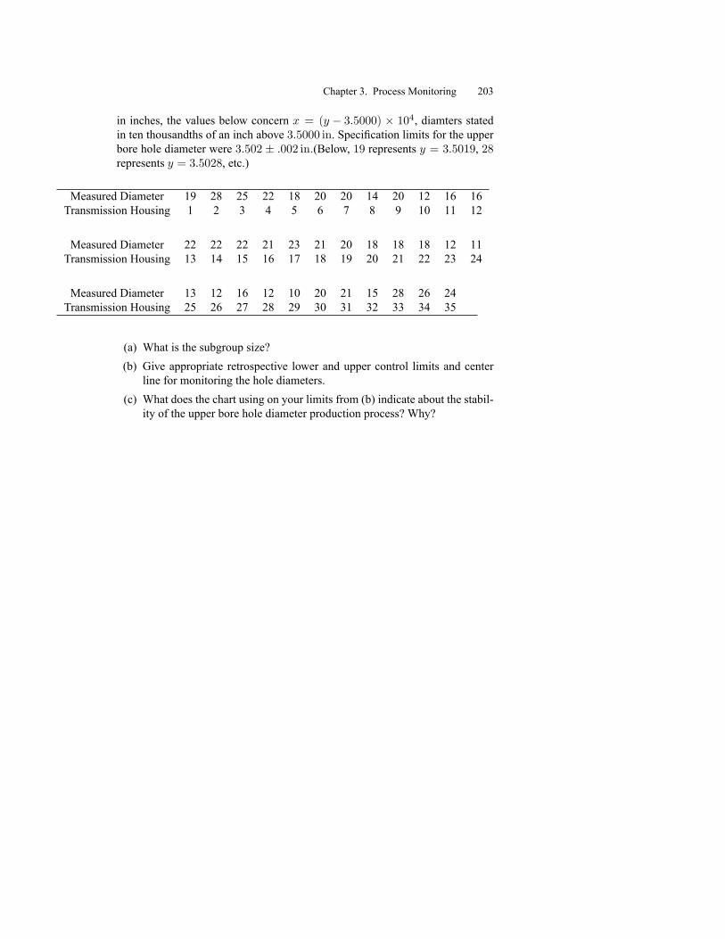
Chapter 3. Process Monitoring 203
in inches, the values below concern x = (y � 3:5000) � 104, diamters statedin ten thousandths of an inch above 3:5000 in. Speci�cation limits for the upperbore hole diameter were 3:502 � :002 in:(Below, 19 represents y = 3:5019, 28represents y = 3:5028, etc.)
Measured Diameter 19 28 25 22 18 20 20 14 20 12 16 16Transmission Housing 1 2 3 4 5 6 7 8 9 10 11 12
Measured Diameter 22 22 22 21 23 21 20 18 18 18 12 11Transmission Housing 13 14 15 16 17 18 19 20 21 22 23 24
Measured Diameter 13 12 16 12 10 20 21 15 28 26 24Transmission Housing 25 26 27 28 29 30 31 32 33 34 35
(a) What is the subgroup size?(b) Give appropriate retrospective lower and upper control limits and center
line for monitoring the hole diameters.(c) What does the chart using on your limits from (b) indicate about the stabil-
ity of the upper bore hole diameter production process? Why?