Statistical Methods for Astrophysics and Cosmologylapi/lectures/SMAC/SMAC_inference.pdf · Statistical Methods for Astrophysics and Cosmology Samples, statistics and estimators A

Andrea Lapi

SISSA, Trieste, Italy

IFPU, Trieste, Italy

INFN-TS, Italy

INAF-OATS, Italy

Statistical Methods for

Astrophysics and Cosmology

A.Y. 2019/2020A. Lapi (SISSA)

room: A-509

phone: 470

email: [email protected]

Website: https://lapi.jimdo.com/

mailto:[email protected]

https://lapi.jimdo.com/

Statistical Methods for Astrophysics and Cosmology

Overview


PART II : Statistical inference

• Samples, statistics, and estimators

• Point estimation and Fisher information

• Interval estimation

• Resampling

• Hypothesis testing

• Information, entropy, and priors

• Kolmogorov-Smirnov nonparametric testing

• Regression and correlation

• Sufficiency and completeness


Samples, statistics and estimators


Decision and inference

Science is, at least in a broad sense, a decision process,

often based on small-data samples. For example:

• measure a quantity (parameter estimation) → given

some data, what is the best estimate (including uncertainty) of a particular parameter?

• search for correlations → are two measured variables correlated with each other,

implying a possible physical connection?

• test a model (hypothesis testing) → given data and one or more models, are our data

consistent with the models? Which model best describes the data?

Statistics are summarizing properties of the data, constructed from them, that constitute

the basis toward decision-making.




So far, we have focused on considering given probability distributions for a random

variable X, and on using them to compute various quantities. Now we are going to

consider the case where the probability distribution for some random variable X is at

least partially unknown (e.g., its parameters); then we will focus on the prescriptions

to make some statement about the unknown quantities given a particular set of

measured values X=x. In other words, the goal of statistical inference is to take the

outcome of an experiment to infer something about the validity of one or more

hypothesis.

If we combine the random variables related to observables into a vector X and the

parameters into a vector then we have a pdf fX(x;). The idea is that when we

perform an experiment, we get specific values X=x, and we can use in a way fX(x;)

to infer something on .




A case of particular interest is when the variables Xi in X are independent and

identically distributed, i.e., they form a random sample. Then

fX(x;) = i f(xi;)

To illustrate the different approaches to the problem, in the sequel we will consider the

following example: suppose we have n data points xi, drawn from independent

Gaussian distributions with the same unknown mean and different known variances

i2. We are thus basically making n independent measurements of the same unknown

, each with its own error i2. How can we use the measured values xi to say

something about the ?




Bayesian point of view: posterior pdf

The Bayesian perspective treats the inherently random realization x and the unknown

parameters on the same footing, both representing uncertainty or lack of

knowledge. The sampling function is thus better written as

f = f (x|)

a pdf for x values given . If your apriori knowledge about is reflected by a pdf f(),

then the joint pdf of having parameters and observed data x is

f (x,) = f (x| ) f ()




Actually we are interested in the a-posteriori knowledge of given that we made the

measurements x, which is the conditional probability

f (|x) = f (x,)/f(x) = f (x|) f () / f(x)

This is a form of Bayes’s theorem. Naming conventions:

f () is the prior pdf

f (|x) is the posterior pdf

f (x|) is the sampling pdf, or likelihood pdf when considering its dependence

f(x) = d f (x|) f () is a normalization factor

Caveats on the Bayesian approach: conceptual subtlety to assigning probabilities to

unknowns which are not repeatable experiments; some arbitrariness in the prior pdf.




Coming to our working example, the likelihood is

Now when we substitute into Bayes’s theorem, we will get a pdf for that is Gaussian

too. We can write this transparently by completing the square and writing

and solving for 0({xi}), 2({xi}), and 0

2({xi}), the names of which have been

deliberately chosen.




Expanding both sides and equalizing, we find

which is actually independent of the {xi},

which is irrelevant here, and

which is a sort of weighted mean.




Then the likelihood function can be written as

and the posterior pdf reads

where the proportionality constant can be worked out from the normalization condition

on the posterior pdf. As you can see the essential information about the outcome of

the experiment is encoded in the weighted mean 0({xi}) !




Frequentist point of view: optimal estimates

In the frequentist approach, we are just limited to the use of the likelihood f (x|); this

often reduces to try getting an optimal estimate of our unknowns.

Coming to our working example, the best thing we can do is trying to estimate the

value of , and to consider what is the best estimator to use. For simplicity let’s

restrict ourselves to linear combination of the random variables

= i a i Xi

We would like that the expectation value of the estimate < > =i a i < Xi > = i a i

coincides with the true value (unbiased estimate), so implying i a i = 1.




The variance of the estimate is

Var()= i j a i aj Cov(Xi Xj) = i a i2i

2

The optimal estimate would be the unbiased estimate with the lowest variance. We

can use the method of Lagrange multipliers, by minimizing i a i2i

2 + (i a i -1)

with respect to {a i } and to . This gives a i = - /2 i2 and i a i =1, so yielding = -2/

i i-2 . The optimal estimate is found to be

= i i-2 Xi / i i

-2

with variance Var() =1/ i i-2 . Note that this is precisely the weighted mean that

showed up in the posterior pdf for the Bayesian approach, and its variance is the

width of the posterior pdf in the case of a uniform prior.




Statistics and estimators

Given a random vector X, a statistics T(X) is any function of the random variables.

The statistics T(X) is itself a random variable, that in a particular realization where

X=x takes on values T(x). Often a statistics is used to get an estimate of a parameter

; in that case we say that T(X) is an estimator for .

A statistics T(X) is called an unbiased estimator for if

<T(X)> =

otherwise B=<T> - is called the bias of T. For example, consider a random sample X

drawn from any distribution with < Xi > = . Then we know that the statistics T(X) = X

= i Xi /n satisfies < X > = . Thus X is an unbiased estimator of .




Consider now an exponential pdf with unknown parameter :

f(x; ) = exp(- x)

We know that 1/ is the expectation value for an exponential pdf, so X is an unbiased

estimator of 1/. However, one can show that 1/X is a biased estimator of , because

in general

<1/X> 1/<X>

E.g., for a random sample of size n following an exponential pdf we have

<1/X> = n n dx1…dxn exp[-(x1+…+xn)] / (x1+…+xn)




Change to variables

yi = n j=1i xj

so that the limits of the integrals become 0<yi<yi+1 for i<n and 0 <yn<

We get

<1/X> = n dyn exp[-yn] /ynn-2 (n) = n (n-1)/ (n) = n /(n-1)

Of course, in this case we can just multiply by a constant to get an unbiased estimator

for , i.e.

(1-1/n) (1/X)




It is instructive to look at the average squared error for an estimator T of a parameter :

<[T(X)- ]2> = <[(T-<T>)+(<T>- )]2> = <(T- <T>)2 > + 2 (<T>- ) <(T-<T>)> + (<T> - )2 =

= Var[T] + B[T]2

This is the square of the bias plus its variance. So it is reasonable to look for an unbiased

estimator with the smallest possible variance !

The square root of the variance for an estimator in known as its standard error

T = Var[T]




Consistency

A sample of statistics Tn is called a consistent estimator for if and only if it

converges in probability to it, i.e.,

Tn→

For example, the quantity (n-1) S2 /n = i (Xi -Xn)2 is a biased estimator of the

variance since <(n-1) S2 /n> = (n-1) 2 /n, but it is still consistent since (n-1) S2 /n →

2 as n→ .

On the other hand the sequence Tn =Xn is obviously an unbiased estimator of the

mean but does not converge to anything, so it is not a consistent estimator.


Point estimation and Fisher information


Estimating with moments

One method for estimating the parameters of the likelihood is to express them as a

combination of its moments

<Xk> = dx f(x|) xk

E.g., for a Gaussian likelihood we have the two parameters and . The moments of the

likelihood are <x> = and <x2> = 2+ 2; solving for and we can thus define the

method-of-moments estimates of and as

= <X> =X 2 = (<X2> -<X>)2 = (n-1)/n * S2

Note that < >= while <2> = (n-1)/n * , so is unbiased while is biased.




Maximum likelihood estimator

One method for obtaining an estimator of the parameter is to pick up the value which

maximizes the likelihood f (x|), where x are the observed data. This seems reasonable

because it gives the parameter value for which the actual data were most likely. However,

there is still something a bit fishy, since the likelihood function is not a probability

distribution for , but rather for x with a dependence from . The mle is defined as

df (x|) /d|= = 0

The Bayesian approach tells why the mle is a good idea. Since f (|x) f (x|) f() from

Bayes, we see that if the prior pdf f() for is uniform, then the mle also maximizes the

posterior pdf f(|x).




Since the max likelihood estimate depends on x, it can be thought as a random

variable, hence as a statistics constructed from the random sample X. In this respect

two considerations give support to the use of the maximum likelihood estimate:

1. Suppose 0 is the true value of a parameter , and X is a random sample of size n.

then the true parameter maximizes the likelihood in the limit n → , i.e.,

limn → f(x|0) > f(x|)

2. The maximum likelihood estimator converges in probability to the true parameter,

i.e., it is a consistent estimator, i.e.,

→ 0

So essentially in the large n limit, the true value becomes the mle and viceversa.




Log-likelihood

In practice, it is easier to compute the maximum likelihood estimate using the

logarithm of the likelihood function and considering it as a function of , i.e.,

L() = ln f (x|)

For example, consider the exponential distribution. The loglikelihood function is

L() = n ln() - i xi

Differentiating and setting this to zero gives the (biased) estimator

= n /i xi = 1/X




Method of least squares

Suppose you have two random variables X and Y related by a known functional

dependence g such that

Y = g(X,)

where is a vector of parameters. Assume that the variables follow a normal

distribution with X << Y . The method of least squares is based on the log-likelihood

L() = - i=1…n [yi-g(xi,)]2 / i2 + cost.

If the variance are equal, the maximum likelihood method tells us that it is enough to

minimize the squares of residuals given by i=1…n [yi-g(xi,)]2




As a relevant example, suppose to fit the data with a straight line. In this case

Y=aX+b. Find the parameters of the best fitting (“regression”) line. Assuming the

same variance 2 for the y values, one has

a i=1…n [yi- (axi+b)]2 = 0 → ai xi2+b i xi - i xi yi = 0

b i=1…n [yi- (axi+b)]2 = 0 → ai xi +nb -i yi = 0

whose solution is the following (where the average is defined as x= (1/n) i xi )

a = [xy-x y] / [x2-x2] b = [y x2- x xy] / [x2 - x2]

a2 = 2 / [x2 - x2] b

2 = 2 x2/ [x2 - x2]




If the variances are not equal, we have to minimize i=1…n [yi-g(xi,)]2 / i2

a i=1…n [yi- (axi+b)]2/ i2 = 0

b i=1…n [yi- (axi+b)]2 / i2 = 0

whose solution is the following

a = [xy-xy] / [x2-x2] b = [y x2- x xy] / [x2 - x2]

where the averages are weighted with a weight i-2 and the variances are

a2 = 1 / i i

-2 [x2 - x2] b2 = x2/ i i

-2 [x2 - x2]




One can also try to fit the data with other shapes, e.g., a polynomial by assuming

Y=a +b X +c X 2 +d X 3 . One finds

i=1…n [yi- (a+bxi+cxi2 +dxi

3)] 2 xik / i

2 = 0 k=0,1,2,3

whose solution is given by the system

a+b x+c x2 + d x3 – y = 0

ax+b x2 +c x3 + d x4 – yx = 0

ax2+b x3 +c x4 + d x5 – yx2 = 0

ax3+b x4 +c x5 + d x6 – yx3 = 0




Other estimator algorithms modifying the least square method that are often used:

Least absolute residuals (LAR) → minimize the absolute difference of residuals,

rather than the square difference, implying that extreme values have a lesser

influence.

Bisquare weights → minimize a weighted sum of squares, where the weight to each

point depends on how far the point is from the fitted line. Points that are farther from

the line than would be expected by random chance get zero weight.

As the least square method corresponds to finding the mle for a random sample

drawn from a normal Gaussian f(x) exp[-(x-)2], these other methods can be shown

to arise when other pdf are considered; e.g., the LAR corresponds to the double

exponential pdf f(x) exp[-|x-|]







Robust estimators

Let {Xi} be a random sample drawn from a pdf f(xi-) where is a parameter. The

corresponding log-likelihood will be

L’() = i f’(xi - )/ f(xi - ) = i (xi - )

E.g., if f(x) is Gaussian, then (x)=x, while if f(x) is the Cauchy distribution (x)=2x/(1+x2).

Clearly the mle found by solving the equations i (xi - ) =0 will be very different for different

initial pdf f(x). E.g., for a Gaussian we find that the mle is the sample mean x = (1/N) ixi ,

which estimates optimally the median of the Gaussian but poorly that of the Cauchy pdf.

An estimator that is fairly good (small variance) for a wide variety of distributions (but not

necessarily the best for any) is called robust.




Quality of an estimator: Cramer-Rao bound

The variance of an unbiased estimator Var(Y) = <[Y- ]2> can be interpreted as a loss

function, measuring the risk of making a poor estimate. So choosing an estimator that

minimizes the variance is highly desirable. An estimator T(X) is called an unbiased

minimum variance estimator (mve) of if it is unbiased, i.e. <T(X)> = , and if the

variance of T is less than or equal to the variance of every other unbiased estimator

of .

Looking for mve among all estimator is a complex issue. A first look at the problem

comes by introducing the concept of Fisher information in terms of the log-likelihood

L() = ln f (x|) as

I() = Var[L’()]




First of all note that

<L’()> = dx f(x,) ln f(x,) = dx f(x,) = 1 = 0

Then the Fisher information is actually

I() = <[L’()]2>

The following identity holds

0 = d <L’()> = d dx f(x,) ln f(x,) = dx f(x,) ln f(x|) + dx f(x|) 2 ln f(x|)

so that

I() = - <L’’()>




For example, consider the normal distribution with mean and variance 2 . Then

L() = -(x- ) 2 / 22 - ln(22 )/2

so taking derivatives we have L’() = (x- ) / 2 from which we can easily cross-check

that <L’()> = 0 and

L’’() = -1/ 2

from which we compute the Fisher information

I() = 1/ 2




Interestingly, for a random sample of size n one has L X() = ln f (x|) = ln i f(xi;) = i

ln f(xi;) and so I X() = -<L X’’()> = -i <L’’ ()> = n I().

Now for a general estimator T(X) of a parameter , the variance is given by

Var(T|) = <[T - <T>()]2|>

This has a similar structure to the Fisher information for the sample, since both are of

the form <[a(X)] 2| > = a • a , where we have defined the dot product

a • b = dx f(x, ) a(x) b(x)

From the Cauchy-Schwarz algebraic inequality (a • a) (b • b) | a • b |2 one has




Var(T|) n I() [<[T - <T>()] L’()|>]2 = [<T L’()| > - <T>() <L’()>]2 =

= [ dx T(x) f(x, ) ]2 = [ dx T(x) f(x, )]2 = [d<T>]2 = [<T()>’ ]2

So we have obtained the so-called Cramer-Rao bound

Var(T|) [<T ()>’]2 /n I()

In the special case when T is an unbiased estimator of then <T()> = and

Var(T|) 1 /n I()

The variance of an estimator can be no less than the inverse of the Fisher information

of the sample.




For a Gaussian likelihood with mean and variance 2 , and an estimator like the

sample mean X the bound tells us that

Var(X|) 1 /n I() = 2 /n

In this case we know that the bound is saturated, and the sample mean is the lowest

variance unbiased estimator of the distribution mean .

When the Cramer-Rao bound is saturated, the estimator T is said to be efficient.

Otherwise the ratio of the bound to the actual variance is called efficiency of the

estimator. Another selling point of the maximum likelihood estimate is that it becomes

efficient in the limit of infinite sample size. Also, the distribution of the mle converges

in probability to a Gaussian with zero mean and variance specified by the bound:

n [ - ] → N(0, 1/I())




Fisher information matrix

We can now ask how the likelihood pdf performs in the vicinity of the maximum

likelihood estimate of the parameters. One trick would be to Taylor expand f(x|) near

its maximum, but since f(x|) 0 this can cause problems if we extrapolate too much.

So instead expand the log-likelihood

L() L() + L’() (- ) + ½ L’’() (- )2 +…

Taking the expectation value, now we know that <L’()> =0 and <L’’()> <0. If we

truncate the expansion at the first nontrivial order we get

f(x|) f(x| ) exp[- ½ <|L’’()|> (- )2]




which is a Gaussian with width <|L’’()|> -1/2 . The second derivative <|L’’()|> is the

one dimensional version of what is known as the Fisher information matrix. More

rigorously, if one has multiple parameters = {1, 2,…, m} it is true that

<L()/i > = dx f(x|) / i = ( / i) dx f(x|) = 0

Since L()/i is a random vector, we can construct the (symmetric) variance-

covariance matrix, known as Fisher matrix, with elements

Fij = <L()/i L()/j>

Now we can differentiate with respect to j to get the identity

0 = ( / j) dx f(x|) ln f(x|) / i = dx f(x|)/j ln f(x|) / i +

+ dx f(x|) 2 ln f(x|) /ij = < 2 L()/ij > + Fij




So an equivalent way of writing the Fisher information matrix is

Fij = - < 2 L()/ij >

The Fisher matrix gives an estimate of the uncertainties of the parameters. Recall

indeed from the Cramer-Rao bound that the mle from a sample of size n>>1 tends

to a normal distribution; in the multiparametric case this is a multivariate normal

n [ - ] → N[0, F() -1]

The matrix inverse F() -1 of the Fisher matrix is the variance-covariance matrix of the

limiting distribution. The multiparameter version of the Cramer-Rao bound is

Var[T i(X)] (1/n) [F() -1] ii




Thus the diagonal elements of the inverse Fisher matrix provide lower bounds on the

variance of the unbiased estimators of the parameters. This is the justification for the

common practice of quoting such quantity as one-sigma uncertainty on the parameter

estimate.

Note that if the Fisher matrix has off-diagonal elements, then it is mandatory to take

the diagonal elements of the inverse Fisher and not the inverse of the diagonal

elements of the Fisher matrix, since typically

[F -1] ii 1/ Fii

This is thus a stronger bound than one would get by assuming all of the “nuisance”

parameters to be known and applying the usual Cramer-Rao bound to that of interest.




Maximum a-posteriori estimate and Hessian matrix

To perform a point estimate in the Bayesian approach one could simply find the value of

which maximizes the posterior f(|x), known as maximum a posteriori estimate (map). Note

that if we perform a change of variables in the parameters, the mle does not change, while

the map does, because the likelihood f(x|) is not a density in , while the posterior f(|x)

is. Analogously to what we have done with the likelihood expansion around the mle, one

can expand the posterior in the vicinity of the map estimate . One will obtain then

in terms of the Hessian matrix H with elements Hij = [2 ln f(|x) /i j ]= Plainly, the width

of the marginal pdf for a particular parameter is

Var[i ] = [H-1 ]ii

f(|x) f(|x) exp[- ½ (- )T H (- ) ]


Interval estimation


Beyond finding the most likely parameter value and describing the shape of the

likelihood around that value, an important task in parameter estimation is to provide

an interval that we associate quantitatively with likely values of the parameter.

Bayesian plausible intervals

From the Bayesian point of view, where a particular sample instance x results in a

posterior pdf f(|x), one would have a straightforward definition for a plausible interval

in which we think is to lie with some probability 1-

iu d f(|x) = 1-

So this means the probability that the estimates are under the posterior pdf, between

l and u is 1-.


Interval estimation


This leaves the freedom to choose where the interval begins. Some convenient

choices are:

-) Lower limit P(l < ) = 1-

-) Upper limit P( < u) = 1-

-) A symmetric two-sided interval P( > l) = P(u > )= /2

-) A interval centered on the mode of the posterior pdf P( - /2 < < + /2)= 1-

-) The narrowest possible intervals, i.e., of all the intervals with P(i < < u) = 1-

pick up the one that minimizes u - i

Note that the prescription above is unique for a given posterior pdf, but recall that to

obtain that pdf we need to use whatever information we have about the problem to

construct the appropriate prior pdf f().


Interval estimation


Frequentist confidence intervals

In the frequentist picture, we can only design a procedure to generate an interval

such that if you collect many random datasets and make such an interval from each,

some fraction of those intervals will contain the true parameter value: this is known as

a (frequentist) confidence interval. It is defined as a pair of statistics L=L(X) and

U=U(X) chosen so that the probability that the parameter lies between them is 1-

P(L< <U) = 1-

It is important to stress that the probability is referred to the randomness of the

statistics L and U, and not to . From the frequentist perspective we cannot talk about

probabilities for ; it has some specific value, even if it is unknown. Given a particular

realization x of the sample X, we have a confidence intervals between L(x) and U(x).


Interval estimation


One method to construct the confidence intervals is to choose a statistics T(X;)

dubbed pivot variable, whose pdf is a known function of the parameters, and find an

interval using

P(a< T(X;) <b) = 1-

By solving algebraically the inequalities a< T(X;) and T(X;)<b for , one should be

able to write

P(L(X)< <U(X)) = 1-

However, note that this construction is not unique; different choice of the pivot

variable will give different confidence intervals.


Interval estimation


Now to illustrate the pivot variable method, consider the case where X is a sample of

size n drawn from a normal distribution with both mean and variance unknown,

where we want a confidence interval on .

The pivot variable should depend on and X but not on , so taking

Z = (X-)/ (/n)

will not work. Fortunately, we know from Student’s theorem that the quantity

T = (X-)/ (S2/n)

obeys a t-distribution with n-1 degrees of freedom, i.e., fT(t;n-1).


Interval estimation


This works as a pivot variable, since S2 = i (X i -X)2 /n depends only on the sample,

and requires no knowledge of or .

In general, the (1-) 100th percentile of the distribution t,n is easy to compute

1- = P(T<t,n) = -t,n dt fT(t;n)

Since we want a two-side

confidence interval, actually we

need t/2,n and t1- /2,n ,

but because of the symmetry

in the t-distribution we can use that

t1- /2,n = - t/2,n


Interval estimation


Turning back to our pivot variable T, which is t-distributed with n-1 degrees of freedom, we

find

1- = P(-t/2,n-1 < T< t/2,n-1) = P(-t/2,n-1 < (X-)/ (S2/n) < t/2,n-1)

which, solving for the two inequalities gives the confidence intervals

P[X - t/2,n-1 (S2/n) < < X + t/2,n-1 (S2/n)] = 1-

Thus typically the Student distribution is exploited to give confidence intervals to Gaussian

estimates, especially in the cases of a sample with few data points.


Resampling


The best way to establish the properties of a population is to examine each and every

member, make the appropriate measurements, and record their values.

The alternative is to select many samples, and to estimate their statistical properties.

Plainly, by taking different samples we might record quite different values. Finding out how

different, it is the best way to determine how precise our estimates are.

There are two practical procedures to do this known as bootstrap and jacknife; these can

be used not only to get an estimate of a parameter but also to estimate its variance when

the latter is difficult to get (e.g., correlated data), and check for biases.


Resampling


Bootstrap

The bootstrap treats the original sample of values as a stand-in for the population and

resamples from it repeatedly, with replacement, computing the desired estimate each time:

• observe a sample X=x={x1… xn} and compute the estimate (X)

• for i=1…s where s is the number of bootstrap samples to be generated:

o generate a bootstrap sample Xi = xi ={x i1… x i

n} by sampling with replacement

from the observed dataset

o compute i = (Xi) in the same way that you calculated the original estimate

• compute the bootstrap mean and variance

* = (1/s) i=1…s i S* = [1/(s-1)] i=1…s ( i - *)2


Resampling


Suppose that the measured data come from a cumulative distribution function F(x). In an

ideal world, we would just get more samples from F and then evaluate the variance of our

estimate with these new samples. In reality we do not know this and so we cannot. What

boostrap does is to replace F with an empirical distribution which is an estimate of F. The

number of bootstrap sample s needs to be large but since the error in evaluating the

variance decreases like 1/s there is no point in making s too big. A good technique is to

plot the estimate of variance against s to see whether it has settled down to some value.


Resampling


Example: Bhavsar (1990) estimated via bootstrap the uncertainty in measuring the slope of

the galaxy angular two-point correlation function w() for radio galaxies.

Left: a least square fit to the slope gives -0.19. Right: the distribution of slopes obtained by

bootstrapping the sample with 1000 trials; the slope is less than zero (signal is present) for

96.8 percent of the trials.


Resampling


Jacknife

The jacknife is a more orderly version of the bootstrap.

• observe a sample X=x={x1… xn} and compute the estimate (X)

• for i=1…n :

o generate a jacknife sample X-i = x-i ={x1… xi-1 xi+1…xn} by leaving out the i-th

observation

o compute -i = (X-i) in the same way that you calculated the original estimate

• compute the jacknifed mean and variance

*= (1/n) i=1…n -i S*= [(n-1)/n] i=1…n ( -i - *)2


Resampling


The jacknife is a good method to compute not only the variance of an estimate, but also its

bias. The jacknife estimate of the bias is given by B= (n-1) (*- ) and the bias corrected

jacknife estimate reads

+= - B = n - (n-1) *

This comes about because, for many statistics, B() a/n + b/n2. Then B( -i) a/(n-1) +

b/(n-1)2 and likewise for B(*). Thus

 = (n-1) <(*- )> (n-1) {a[1/(n-1)-1/n] + b [1/(n-1)2-1/n2] = a/n + b(2n-1)/n2 (n-1) B()

so the jacknife bias estimates the true bias up to order n-2. This implies:

B(+) = B() – a/n + b/n2 - a/n – b(2n-1)/ n2 (n-1) -b/n(n-1)


Resampling


Example: Draw 10 samples from a normal

distribution and calculate variance. Do this for

1000 trials, and the result is the blue histogram

on the top panel. The mean variance is

0.89999 less than the true 1.0, because of the

infamous 1/n vs 1/(n-1) issue…

Now calculate variances for each of 1000

jacknife trials, resulting in the red histogram of

the bottom panel. The peak has shifted to

larger values; in fact, the mean variance is

0.9834, much closer to the true value 1.0.

Bias has been removed (reduced) !


Hypothesis testing


So far we have considered how to get handle of parameters in a probability

distribution given that we had a sample drawn from that, and found a particular

realization. Now we wish to consider how to use the realization of the sample to

distinguish between two competing hypotheses about what the underlying distribution

is. For the sake of simplicity we will assume there is only one family f(x,)

parameterized by which lies somewhere in a region and then take the

hypotheses to be

H0 → the distribution is f(x,) where 0

Ha → the distribution is f(x,) where a

Typically H0 represents the absence of the effect we are looking for, and is known as

null hypothesis, while Ha represents the presence of the effect, and is known as

alternative hypothesis.


Hypothesis testing


A hypothesis test is simply a rule for choosing between the two hypotheses

depending on the realization of the sample X=x. Stated more generally we construct

a critical region C which is a subset of the n-dimensional sample space . If X C

we reject the null hypothesis and favor Ha; if X C, we accept the null hypothesis

and favor H0.

Of course, since X is random, there will be some probability P(X C ; ) that we will

reject the null hypothesis, which depends on the value of . If the test were perfect,

that probability would be 0 if H0 were true (i.e., for any 0) and 1 if Ha were true

(i.e., for any a) but we would not be doing statistics. So in practice there is some

chance we will choose the wrong hypothesis, i.e., some probability that, given a value

of 0 associated to H0, the realization of our data will cause us to reject H0 , and

some probability that, given a value of a associated to Ha, the realization of our

data will cause us to accept H0.


Hypothesis testing


We say that:

If H0 is true and we reject H0 → Type I error or false positive

If Ha is true and we reject H0 → true positive

If H0 is true and we accept H0 → true negative

If Ha is true and we accept H0 → Type II error or false negative

Typically, a false positive is considered worse than a false negative, so we decide

how high a false positive probability we can live with, and then try to find the test

which gives the lowest false negative probability.


Hypothesis testing


Given a critical region C, we would like to talk about the associated false positive

probability and the associated false negative probability 1- (while is called power

of the test), but we have to be careful since H0 and H1 are in general composite

hypotheses. This means each of them does not correspond to a single parameter

value and thus to a single distribution, but rather to a range of values 0 or

a. So may depend on the value of . We take the false alarm probability to be

the worst case scenario within the null hypothesis

= max0P(X C ; )

This is called the size of the critical region C, and sometimes also significance of the

test, which is a bit counterintuitive; a low value of means the probability of a false

positive is low, which means a positive result is more significant than if were higher.

It is the probability that we will falsely reject the null hypothesis H0 ,…


Hypothesis testing


…maximized over any parameters within the range associated to H0 . On the other

hand, since the alternative hypothesis almost always has a definite parameter

associate with it, we define the probability of correctly rejecting the null hypothesis as

C= P(X C ; ) for a

We explicitly write this as a function of the critical region C, since we might want to

compare different tests with the same false alarm probability (critical regions with

the same size ) to see which one is more powerful.

As an example, let X be a random sample of size n from a normal distribution, where

the null hypothesis H0 is =0, and the alternative hypothesis Ha is >0. For simplicity,

let us assume that the variance 2 is known; alternatively, when the sample size is

large we can use S2 as an estimate.


Hypothesis testing


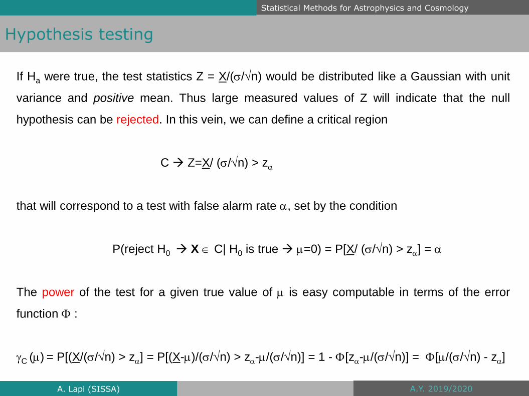
If Ha were true, the test statistics Z = X/(/n) would be distributed like a Gaussian with unit

variance and positive mean. Thus large measured values of Z will indicate that the null

hypothesis can be rejected. In this vein, we can define a critical region

C → Z=X/ (/n) > z

that will correspond to a test with false alarm rate , set by the condition

P(reject H0 → X C| H0 is true → =0) = P[X/ (/n) > z] =

The power of the test for a given true value of is easy computable in terms of the error

function :

C () = P[(X/(/n) > z] = P[(X-)/(/n) > z-/(/n)] = 1 - [z-/(/n)] = [/(/n) - z]


Hypothesis testing


The power of the test as a function of is

illustrated on the right. The power goes from

the value of the significance when =0, and

then increases with () > when >0. This is

a very desirable property, since the test should

be more likely to reject H0 when it is false than

when it is true! A test with this property is

called unbiased.

For definiteness, let’s choose a significance =0.05 ; then using the Gaussian distribution

P[Z=X/ (/n) > z] =

will imply z = 1.645 . And the power of the test is () = [/(/n) – 1.645] .


Hypothesis testing


p-values

In this example, given a data realization x, and specifically a sample mean x, we will

reject the null hypothesis if x > z/n. This means there will be some values of the

false alarm probability for which we reject H0 and some for which we do not. One

convenient way to proceed is quoting the most stringest significance level for which

H0 would be rejected. In other words, we ask, given a measurement (in this case x)

how likely is that we would find a measurement at least as extreme, just by accident,

if the null hypothesis were true. In the previous example we have

p = P[X>x; =0] = 1 - [x/(/n)] = [-x/(/n)]

This is known as p-value. A lower p-value means that the results were less likely to

have occurred by chance in the absence of a real effect. Typically p<0.05 is good!


Hypothesis testing


Pearson’s Chi-squared tests

Both the false alarm rate and the p-values are ways of talking about how inconsistent

the data are with the null hypothesis. Another similar test is the goodness-of-fit or

Pearson’s chi-squared test: we measure how closely the actually collected data come

to the most likely values, and how likely we were to deviate by that much or more, if

the model were actually correct.

As an example, consider the case where the null hypothesis tells us that our random

data vector X is made up of n independent random variables with means i and

variances i . Then we know that the test statistics

Z i = (Xi - i)/i

is a standard normal.


Hypothesis testing


Thus

Y = i Z i2= i [(Xi - i)/i ]

2

is a 2(n) random variable. If the measured data gives a Y=y much larger than

expected for a 2(n) distribution, this casts doubts on the null hypothesis. In other

words, we construct a test with false alarm rate probability by the condition

P(Y > 2n,) =

where 2n, is the 100 (1-)th percentile of the 2(n) distribution.

Other tests based on this very same approach are the likelihood ratio, Wald, and Rao

score tests. We will now analyse them in some detail.


Hypothesis testing


More in general, consider a likelihood f(x|) . A test often used is the so called

likelihood ratio test, based on the quantity (x) = f(x|) / f(x|) with is the mle of the

parameter. It can be demonstrated that asymptotically it converges in distribution to

2L = -2 ln (x) → 2 (1)

For finite n we assume this is approximately true and compare 2L to the 100(1-)th

percentile of the 2 (1) distribution to get a test with false alarm probability .

E.g., consider a sample of size n drawn from a Gaussian with mean and variance

2, for which the mle is the sample mean x. Then the likelihood ratio is (x) = exp[-n

(-x)2 /22] . Since the sample mean X is distributed as a Gaussian with mean and

variance 2/n we have

-2 ln (x) = (X- ) 2 / (2 /n) 2 (1)


Hypothesis testing


Another possibility is to consider the result that the quantity n [(X)- ] converges in

distribution to a Gaussian with mean zero and variance 1/I(), and construct the

statistics

2W = n I() [(X)- ] 2

Comparing this to the percentiles of 2 (1) is known as Wald test.

E.g., for a Gaussian we have I() = 1/2 and Wald test statistics

2W = (n/ 2) [X - ]2 2

L 2 (1)

being of the same form of the likelihood ratio test.


Hypothesis testing


Another possibility is to consider the log-likelihood L() = ln f(x|). We know that

<L’()> = 0 and that Var[L’()] = n I(). So we can construct a test statistics which, in

the limit that the sum of scores is normally distributed, becomes a 2 (1) , i.e.,

2R = [L’()] 2 /n I()

Comparing this to the percentiles of 2 (1) is known as Rao scores test.

E.g., for a Gaussian we have L’() = n (X- )/2 and Rao scores test statistics

2R = (n/ 2) [X - ]2 2

L 2

W 2 (1)

which is again of the same form of the preceding tests, and exactly 2 (1) distributed.


Hypothesis testing


Most powerful test: Neyman-Pearson lemma

The most powerful test between two one-point hypotheses H0 and H1 can be constructed

from the likelihood ratio (x) = f(x|H0) / f(x|H1) in the following way. We define the critical

region C so that xC if and only if (x) < k where k is defined by

P[(x) < k|H0] = C dx f(x|H0) =

which ensures that the critical region is of size given by the significance . Now we prove

that the power of this test

C =P[(x) < k|H1] = C dx f(x|H1)

is greater than for any other test with the same significance.


Hypothesis testing


Proof

If A is some other critical region of size than we have to prove that C > A . To this purpose

split A and C in terms of their overlap region C A as

C = (C A) (C A) A = ( C A) (C A)

The contribution to C A cancels out of any comparison, so we have just to prove that

C A > C A . Now by definition (x) <k in C and (x) >k in C implying that

C A = C A dx f(x|H1) > C A dx f(x|H0) /k

C A = C A dx f(x|H1) < C A dx f(x|H0) /k

Now = C dx f(x|H0) = C A + C A and = A dx f(x|H0) = C A + C A so that

C A dx f(x|H0) = C A dx f(x|H0) implying C A > C A , hence proving C > A .


Hypothesis testing


Suppose now that H0 is a one-point hypothesis while H1 is a composite hypothesis which

allows for a range of values of the model parameters but comes with a prior f(|H1). If we

define a test which rejects H0 when

(x) = f(x|H0) / f(x|H1) = f(x|H0) / d f(x|) f(|H1) < k

the Neyman-Pearson lemma tells us that this is the most powerful test of H0 over H1 . This

is most powerful in the sense of maximizing the power function

C(H1) = P[(x) < k|H1] = C dx f(x|H1) = C dx d f(x|) f(|H1) = d () f(|H1)

We note that the above is precisely the test statistics based on posteriors from Bayes

[f(x|H0)/f(x|H1)] × [P(H0)/P(H1)] × [f(x)/f(x)] = P(H0|x)/P(H1|x)


Hypothesis testing


Reduced Chi-square

Consider now H0 to be a composite hypothesis corresponding to a family of models,

such that the Xi are to follow normal distributions with means i () and variances i()

depending on a m-dimensional vector of parameters . Then the 2-statistics

corresponding to a particular set of parameter values is

Y() = q(X, ) = i [Xi - i ()]2 /i2()

If H0 is true and are the actual parameter values, Y() is 2(n) distributed. But

suppose that we do not know the parameter values, and we have collected a data

vector X=x. We can choose as our best estimate of the parameters the values

jY() = 0 for j=1,2,…,m


Hypothesis testing


If you put these values back into Y, we get the minimized chi-squared values

Y =Y [(X)]

It turns out that, under many circumstances, this statistics obeys a 2(n-m)

distribution, which is called reduced chi-squared. If a model predicts that X are to

follow a Gaussian distribution, we can collect a realization of these data X=x and

construct a test with significance from

P(Y > 2n-m, ) =

As an example of reduced 2 with m=1, suppose H0 says that, for a parameter , the

data are a normal random sample with each mean i = and each variance i = .

Then the chi-square statistics is Y = i (Xi - ) 2 /2 .. The minimum chi-squared is


Hypothesis testing


0 = (2/2) i (-xi + ) = (2/2) (n - i xi)

Thus the corresponding statistics is

(X) = X

i.e., the sample mean. Note that is also the maximum likelihood estimate, since

the likelihood function L() exp(-Y). Substituting into the chi-square statistic, we

get the minimized chi-square

Y = Y( = X) = i (Xi - X ) 2 /2 = (n-1) S2 /2

where S2 is the sample variance. But from Student’s theorem this follows a 2(n-1)

distribution; so we have indeed found that the chi-squared statistics minimized over

m=1 parameter follows a 2(n-1) distribution.


Hypothesis testing


Bayesian hypothesis testing

In the Bayesian framework, the joint pdf for a sample X drawn from a distribution with

parameter can be written f(x,), and we can talk about the posterior probability

P(H1|x) that a hypothesis is true, given an observed sample x. There are few caveats,

however.

Typically, our hypothesis allows to describe the joint pdf for a random sample X

collected in the presence of that hypothesis f(x|H1), and then we can use Bayes’s

theorem to construct the desired probability

P(H1|x) = f(x|H1) P(H1)/f(x)

But this expression depends on P(H1), which is the prior probability that the…


Hypothesis testing


…hypothesis H1 is true, and we might have difficulties in stating it. Another issue in

the Bayesian framework is that the pdf f(x|H1) and f(x|H0) require to specify the

hypothesis a little more precisely than we have done so far (a range like 1 is not

enough). In particular, if one or both are composite hypothesis, we need to state the

pdf associated with the hypothesis for . For instance, marginalizing over yields

f(x|H1) = 1d f(x|) f(|H1)

Finally, the denominator f(x) is the overall pdf for the sample, marginalized over a

complete set of mutually exclusive models, i.e.,

f(x) = f(x|H0) P(H0) + f(x|H1) P(H1) + f(x|H2) P(H2) + …

which we are even less likely to have an handle on.


Hypothesis testing


Odds ratio, Bayes factor, and Occam principle

The usual way to circumvent the latter issue is to calculate not P(H1|x) but the odds

ratio O10, the ratio of the posterior probabilities of the competing models H1 and H0

O10 = P(H1|x)/P(H0|x) = f(x|H1) P(H1)/f(x|H0) P(H0) = B10 P(H1)/ P(H0)

where the ratio of the likelihoods B10 = f(x|H1)/f(x|H0) is known as Bayes factor. The

Bayes factor allows to overcome one of the problems about using a frequentist chi-

square test to assess the validity of a model: adding more parameters to the model

make the fit better, but clearly an overtuned model is scientifically unsatisfying.

Suppose model H1 has one parameter and model H0 has none. Then

B10 = d f(x|,H1) f(|H1) / f(x|H0)


Hypothesis testing


Let’s assume that the likelihood can be approximated as a Gaussian near the mle:

f(x|,H1) f(x| ,H1) exp[- (- )2/22]

We will also assume that this is sharply peaked compared to the prior f(|H1) and

therefore we can replace with in the argument of the prior:

d f(x|,H1) f(|H1) f(x|,H1) f(|H1) d exp[- (- )2/22] = f(x|,H1) f(|H1) (2

2) ½

Then the Bayes factor can be approximated as

B10 = [f(x|,H1)/f(x|H0)] (22) ½ f(|H1)

The first factor is the ratio of the likelihood between the best-fit version of model with

parameters and that with no parameters.


Hypothesis testing


That’s the end of the story in the frequentist approach, and we can see that if H0 is

included as a special case of H1 then the ratio will be always greater or equal than 1,

i.e., the tunable model will be able to find a higher likelihood than the model with no

parameter. But in the Bayesian version, there is also a second factor, called the

“Occam factor”, because it implements the Occam razor, the principle that, all else

being equal, the simpler explanation must be favoured over more complicated ones.

In fact, because the prior f(|H1) is normalized, then [f(|H1)]-1 is a measure of the

width of the prior, i.e., how much parameter space the tunable model is available to it.

For example, if the prior is uniform the Occam factor becomes (22) ½ / (max - min)

Because we have assumed that the likelihood function was narrowly peaked

compared to the prior, the Occam factor is always less than one, and the tunable

model must have a large enough increase in likelihood over the simpler model in

order to overcome this effect.


Hypothesis testing


Example: modelling of radio-source spectra. Left: data, corresponding to a powerlaw

S(f) = k f -1. Right: same data but with an offset error of b = 0.4 units as well as

random noise = 10% Gaussian added.

First take the original data (left hand side) and test the model S(f) = k f -. Each term in

the likelihood product is proportional to

[2( k f i-) 2 ] 1/2 exp [- (S i - k f i

- ) 2 /2 ( k f i-) 2 ]


Hypothesis testing


The log-likelihood contours are shown in the

top panel.

The Gaussian approximation via Fisher

matrix expansion is in the bottom panel.


Hypothesis testing


Now take the data with offset and random noise added (right-hand) and test the original

model without offset and another possible model S(f) = b+ k f - with offset b. Each

likelihood term is

[2( k f i-) 2 ] 1/2 exp [- (S i - b - k f i

- ) 2 /2 ( k f i-) 2 ]

and we pose a Gaussian prior on b of mean 0.4 (we are well informed! ☺). Then

marginalize b out to find the contours reported in figure (solid: model without offset;

dashed: model with offset). The model with offset

does a better job in recovering the true parameter.

But now suppose we are not informed…is a model

with offset (1) a good a priori bet over one without (0)?

To answer, compute the odds ratio [assume P(1)=P(0), i.e.,

agnostic state] by integrating likelihood over parameters:

O10 = B10 P(1)/ P(0) = B10 = 8 → definitely a good bet!


Hypothesis testing


Note that up to now we have adopted a Gaussian prior on the offset b, with known mean

0.4 and stddev , i.e.,

[2 2 ] 1/2 exp [-(b-0.4) 2 /2 2 ]

…a very strong assumption! Suppose we know the

stddev but not the mean , and take the prior on

 as uniform. This is called an hyperparameter, and

is useful to get a posterior distribution for the

interesting parameters (in our case k and )

which includes a range of models. Recomputing

and marginalizing over both b and we get the

solid contours on the right (dashed line is model

with known ): the figure shows there is a tendency for estimating flatter powerlaws if

we do not know much about .


Hypothesis testing


Finally, we can allow a separate offset bi at each frequency, so that each term in the

likelihood product takes the form

exp [-(b i -) 2 /2 2 ] * [2( k f i-) 2 ] 1/2 exp [- (S i - b i - k f i

- ) 2 /2 ( k f i-) 2

and assume again the weak uniform prior on .

The contours (dashed: model above;

solid: original model without offset) tell that

by allowing a range of models via hyperparameters

the solution has moved away from the well-defined

(but wrong) parameters of the non-offset model…

but this is at the cost on much wider error bounds

on the parameters.


Information, entropy, and priors


In the Bayesian approach to parameter estimation, we use some data D to make an

inference based on Bayes’s theorem to construct the posterior pdf

f(|D) p(D|) f()

where the prior distribution f() is expected to reflect the plausibility we assign to

different values of , given our information on the process. Unfortunately, sometimes

it is difficult to convert this information into a prior pdf. Some tricks can be used for

constructing useful prior given seemingly incomplete information.

Jeffreys prior

The simplest prior one may think of is a uniform distribution over the allowed range of

. However, since f() is a pdf, this causes an issue with any change of variables…




If, instead of , we use a parameter (), then

f() = f() |d/d|

so if f() is a constant, f() will not be, in general. The Jeffrey prior is a prescription for

generating a prior pdf from a likelihood function, in a way which is invariant under

reparametrization. Given a log-likelihood L(), we construct

f() I()

in terms of the Fisher information I() = <-L’’()> = <[L’()]2>. Changing variable yields

I() = I() |d/d|2

which gives just the Jacobian needed to transform f() in f().




As an example, for an exponential distribution

f(x,) = exp(- x)

the loglikelihood is L()=ln - x, the Fisher inormation is I() = 1/ 2 and the Jeffreys

prior reads

f() = 1/

For a Gaussian, the Jeffreys prior for is 1/, but for the mean it is uniform.

There is a sort of odd property of the Jeffreys prior, however. To construct it, you need

to know the likelihood, and in some cases this is not simple.




Maximum entropy principle

A way around the issue of constructing a prior when we have incomplete information

is to use the maximum entropy prescription. It suggests to choose the prior which

maximizes the (Shannon) information entropy subject to any constraint

S = - i p i ln p i

where the summation is over all the states of a system with probability pi. The

motivation for this definition is as follows. Suppose there are a number K of discrete

states, each with probability pi . The frequentist interpretation of probability tells us

that if we run the random experiment N times, it will be found in the i-th state N i=N p i

times. The number of different ways to choose which N 1 of the N experiments are …




… in state 1, N 2 are in state 2, etc. is

= N! / N 1! N 2!...N K!

The (thermodynamic) entropy is defined as S ln , the logarithm of the number of

equivalent states that can be constructed. If Ni is large we can use the Sterling

approximation ln Ni ! Ni ln Ni - Ni so

ln N ln N - N - i Ni ln Ni - i Ni = -N i (Ni /N) ln Ni /N= -N i p i ln p i

Since we are looking for S up to a constant we can define

S (ln )/N = -i p i ln p i




Suppose now that only the minimal constraint of a normalized prior is present, i.e.,

i p i =1

Let’s use the method of Lagrange multipliers and minimize

Seff = -i p i ln p i + (i p i -1)

Differentiating with respect to p j and one finds

p j = exp(-1) and i=1K p i =1

so that the distribution is uniform

p i = 1/K




In the continuous case, one defines the information entropy as

S = - dx f(x) ln [f(x)/m(x)]

where m(x) is a measure, called Lebesgue measure, which acts like a density in x.

The above definition is invariant under reparameterization, since changing variable

from x to y one has the same trasformation for f and m.

The other added complication is that varying S with respect to f(x) becomes a

functional derivatives. As an example, one can easily show that if m(x)=1, the

maximum entropy distribution with mean and variance 2 is a Gaussian…


Kolmogorov-Smirnov nonparametric testing


Non parametric tests are used to compare a sample with a reference probability

distribution (or two samples), without assumption about the true distribution. Let F(x)

= P(X 1x) a cdf of a true underlying distribution of data. We define an empirical cdf by

Fn(x) = (1/n) i I (x i x)

where I is an histogram that counts the proportion of

the data below level x. The law of large numbers implies

Fn(x) → <I(X 1 x)> = P(X 1 x) = F(x)

It is easily recognized that this approximation holds uniformly for all x, so that

maxx | Fn(x) – F(x)| → 0




The crucial observation in the KS test is that the distribution of

maxx | Fn(x) – F(x)|

does not depend on F. For given x, the central limit theorem implies that

n | Fn(x) – F(x)| → N(0, F(x) [1-F(x)])

since F(x)[1-F(x)] is the variance of I[X 1 x]. Now it turns out that (a statement

difficult to be proved)

P[n maxx | Fn(x) – F(x)| > t] → H(t) = 1-2 i=1…(-1) i-1 e -2i2 t

where H(t) is the cdf of the Kolmogorov-Smirnov distribution.




Let us reformulate the hypothesis in terms of cdf

H 0 : F=F0 vs H 1 : FF0

Now we can consider the statistics

Dn = n maxx | Fn(x) – F0(x)|

If the null hypothesis is true, then Dn is well approximated by the KS distribution. On

the other hand, suppose the null hypothesis fails. Since F is the true cdf of the data,

by law of large numbers the empirical cdf Fn will converge to F and it will not

approximate F0 . For large n we will have maxx | Fn(x) – F0(x)| > for small enough .

Then one finds

Dn = n maxx | Fn(x) – F0(x)| > n




If H 0 fails Dn > n → for n → . Therefore, to test H 0 we will consider the decision

rule

= H 0 : Dn c vs H 1 : Dn > c

The threshold c depends on the level of significance and can be found from the

condition

= P [ H 0 | H 0 ] = P[Dn > c | H 0]

When n is large we can use the KS distribution to find c since

= P[Dn > c | H 0] 1 - H(c)


Regression and correlation


Pearson correlation coefficient

We are now interested in testing whether two variables are stochastically independent,

and to define statistics that measure the association between two variables. Given

measured datasets {x i} and {yi} we consider the sample covariance

s(x,y) = [1/(n-1)] i (xi - x) (yi - y)

and the Pearson correlation coefficient

r(x,y) = s(x,y)/s(x)s(y)

The correlation satisfies the following trivial properties

r(cx,y) = r(x,y) if c >0 or c<0 and r(x+c,y+c)=r(x,y)




Now suppose we have a cloud of measure points in the (x,y) plane. Fix x as the

predictor and y as the response variable, and try to find the best line y=a x+b passing

through the points: this is a typical regression problem. We know from the least

square method that the regression line minimizing the squared errors is given by

y = y + s(x,y) [x-x]/s2 (x)

and the minimized square error is

s2 (y) [1- r2(x,y)]

r(x,y)=1 if and only if points lie on a line

with positive or negative slope.




The correlation measures the degree of linearity of the sample points. If the data

vectors are uncorrelated then x has no value as predictor of y, and the regression line

is the horizontal line y=y , r(x,y)=0 and the minimized square errors is s2 (y) .

Note that the sample regression line with predictor variable x and response variable y

is NOT the same as the regression line with predictor variable y and response

variable x, except in the extreme cases where all points lie on a line.

If we model the joint distribution of x and y as a bivariate Gaussian, then the

correlation probability tests the significance of a nonzero value of r(x,y). It can be

demonstrated (it is a hard work) that the probability followed by r is a Student’s t-

statistics with n-2 degrees of freedom

t = r (n-2) / (1-r2)




Some examples:

r=0.0050.031 r=0.8610.008

prob. null hypothesis 0.8 prob. null hypothesis 10-8




Caveat 1:

r(x,y)=0 does NOT imply that the variables are uncorrelated, but only that there is not

a linear relation.

Caveat 2:

beware of summary statistics!

Anscombe’s quartet comprises four

datasets with nearly identical simple

statistical properties: same mean and

sample variance in x and y, same

regression line and same r=0.816.




Spearman rank correlation coefficient

The Pearson coefficient assumes that the relation is linear and that the variances on x

and y account for the errors on the data and their intrinsic scatter. However, in general

these conditions are not satisfied if either we have no prior information about the

parent distribution or when statistical errors are different for each datapoint. The

solution is to adopt nonparametric test, typically the Spearman (or Kendall)

correlation: analyse the correlation in the ranks (ordinal number of sorted values)

where variables are distributed uniformly an no prior is needed. The Spearman rank

correlation coefficient is defined as

rs = 1- 6 (n3-n) i [i-ui]2

where [i-ui] is the difference in ranks in the i-th observations. The probability followed

by the Spearman rank correlation coefficient is again a Student’s t with n-1 d.o.f.




A Spearman coefficient equal to 1 results

when the two variables are monotonically

related, even if the relationship is nonlinear.

When data are roughly elliptically

distributed and there are no

prominent outliers, Spearman and

Pearson coefficients are similar.

Spearman coefficient is less sensitive than Pearson

to strong outliers in the tails of the sample, because

Spearman limits the outlier to the value of its rank.




Partial correlation

Given two variables X and Y, if you know they both depend on a third variable Z in the

same way, then you should study how strong is the correlation between X and Y

considering that it can be partially induced by Z (the lurking variable).

It may be of interest to know if there is a correlation between X and Y that it is NOT

due to their common relation with Z. To do this one computes the partial correlation

r(x,y|z) = [r(x,y) - r(x,z)r(y,z)] / [1-r2(x,z)]1/2 [1-r2(y,z)]1/2

that measures the relationship between X and Y while mathematically controlling the

influence of Z by holding it constant. The above correlation can be Pearson or

Spearman.




Example: churches vs. serious crimes (lurking variable is city dimension)




Principal component analysis

Principal component analysis (PCA) is the ultimate searcher for correlation when

many variables are present. It can answer the questions: given a sample of N objects

with n measured parameters for each, what is correlated with what? What variables

produce primary correlations, and what produce secondary via the lurking third (or n-

2) variables? PCA is a algorithm belonging to the family of multivariate statistics, that

operates as follows. It finds a new set of variables

i = j=1…n aij xj

with values of aij such that the smallest number of new variables account for as much

of the variance as possible. The i are the principal components. If most of the

variance involves just a few of the n new variables, we have found a simplified

description of the data.




Example: sample of QSO by Francis & Wills 1999




For each of the 13 variables, normalize by subtracting mean and dividing by stddev.




Construct variance covariance matrix (13 by 13)

Solve the eigenvalue problem to find eigenvalues, which are the variances.

It is seen that the first 3 components contribute about 84% of the total variance. For

eigenvalues to be significant, they must be larger than unity.




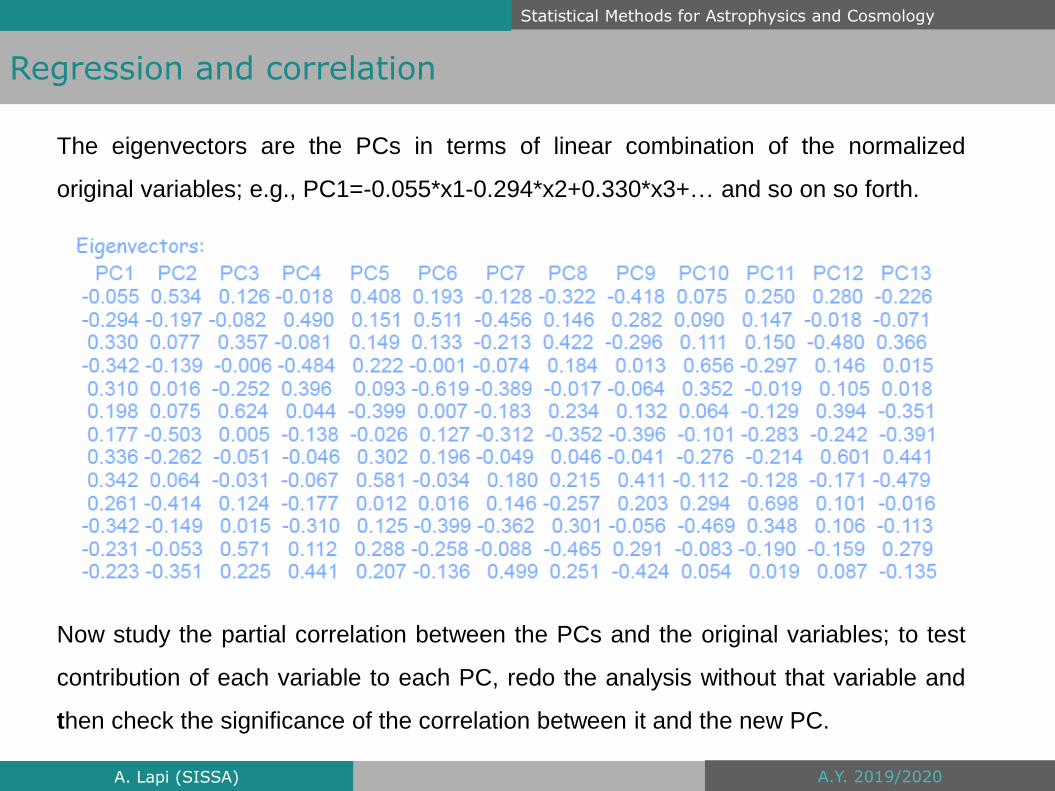
The eigenvectors are the PCs in terms of linear combination of the normalized

original variables; e.g., PC1=-0.055*x1-0.294*x2+0.330*x3+… and so on so forth.

Now study the partial correlation between the PCs and the original variables; to test

contribution of each variable to each PC, redo the analysis without that variable and

then check the significance of the correlation between it and the new PC.




Residual analysis in regression

The appropriateness of a given regression model can be checked by examining

residual plots, i.e., observed-predicted values vs. predicted values.

Ideally, your plot should look symmetrically

distributed, and clustered toward the middle

of the plot, with no clear pattern.




This requirements is not met when:

y-axis unbalanced→ majority of points are below zero line, but a few points are very

above the line. This is a typical problems induced by outliers, observations that lie

abnormally distant from other values in a random sample from a population. Usually

solved by transforming one variable (e.g., with a log-transform)





heteroscedasticity→ residuals get larger as the prediction moves from small to large

(or viceversa). Usually indicates that a variable is missing, and the model can be

improved.





nonlinearity → a linear model does not accurately represent the relation between

variables. Solution is to create a nonlinear model.





strong outliers → the regression has clear outliers. Remove or use appropriate

estimators (e.g., bilinear).


Sufficiency and completeness


We now come back to the issue of searching for the minimum variance unbiased

estimator (mve). We have seen that an estimator saturating the Cramer-Rao bound is

a minimum variance one. But how to search for the mve among all the unbiased

estimator of a parameter? In this context it is extremely relevant the following

concept. An estimator T(X) of a parameter is a sufficient statistics for it if

fX(x, )/fT(t, ) = H(x)

i.e., the likelihood for the whole sample is a -independent multiple of the likelihood

for T. The terminology is appropriate because the statistics T(X) exhausts all the

information about present in the sample; e.g., the conditional pdf of X given T=t and

hence of any other statistics G(X) given T=t does not depend on , and so cannot be

used for statistical inference on that parameter.




We now demonstrate the so called factorization theorem: T is a sufficient statistics for

if and only if the likelihood for X can be factorized as follows

fX(x, ) = k1[t(x),] k2(x)

in terms of two nonnegative functions k1,2

Proof.

Assume the factorization above. Then change variable from x to y(x), with y1(x)=t(x)

and the Jacobian of the transformation being |J|. Then

fY(y,) = k1(y1,) k2(y) |J|

Now we compute the pdf for y1 = t(x)




fT(y1,) = dy2…dyn fY (y,) = dy2…dyn k1(y1,) k2(y) |J| = k1(y1,) dy2…dyn k2(y) |J|

Now the integral does not depend on , so it is only a function m(y1). Thus

fT(y1,) = k1(y1,) m(y1)

If m(y1) = 0 then fY (y1,) = 0. If m(y1)>0 then k1(y1,) = fT (y1,)/m(y1) and the assumed

factorization becomes

fX(x, ) = fT (t,) k2(x)/m[t(x)]

so proving sufficiency. Conversely, If T is a sufficient statistics, then the factorization

can be readily found by taking k1 = fT . The theorem is proved.




Rao-Blackwell theorem

We now prove the so called Rao-Blackwell theorem: let X and Y two random

variables such that Y has a mean and positive variance Y2 , and let <Y|X> Y = (X);

then <(X)>X= and (X)2 Y

2 .

Proof.

We have

(X) = <Y|X>Y = dy y f(y|X) = dy y f(x,y) / f(X)

Then

<(X)>X = dx f(x) (x) = dx dy f(x,y) y = dy y dx f(x,y) = dy y f(y) =

proving the first part of the theorem.




Now consider

Y2 = <(Y- ) 2>Y = dy f(y) [Y-] 2 = dx dy f(x,y) [Y- (x)+(x)-] 2 =

= <[Y- (x)]2 >XY+ <[(x)-]2>X +2 <[Y- (x)] [(x)-] >XY

But the last term is zero because

<[(Y- (x)] [(x)-)] >XY = dx dy f(x,y) [y- (x)] [(x)-] =

= dx [(x)-] f(x) dy f(y|x) [y- (x)] =0

given that (x) = <Y|x> = dy f(y|x) y.




Accordingly

Y2 = <[Y- (x)]2 > XY + (X)

2 (X)2

and this completes the proof of the theorem.

Putting together our results on sufficiency and the Rao-Blackwell theorem, we have that

if Y1 is a sufficient statistics for , and Y2 is an unbiased estimator of based on some

other combination of data, we can make another unbiased estimator

(Y1) = < Y2 | Y1>

which has an equal or lesser variance (Since Y1 is sufficient, f(y2|y1) does not depend on

, so (Y1) is independent of too). So when looking for the minimum variance

estimator, we can confine our attention to sufficient statistics.




Completeness and uniqueness

The Rao-Blackwell theorem tells us that if there is a sufficient statistics Y for , one

function of it is a minimum variance estimator. But we could imagine a case where,

even though we have constructed an unbiased estimator (Y), there might be another

unbiased estimator (Y) which could have a lower variance. One thing we do know

about such a pair of unbiased estimator is that

<(Y) - (Y)> = - = 0

Now in general this does not mean that (Y) = (Y). But suppose that the pdf fY (y,)

of Y has the property that any function u(Y) which satisfies <u(Y)>=0 for all also

satisfies u(Y) = 0. The we know that the function (Y) is unique, and there is only one

unbiased estimator that can be built from the sufficient statistic, and this is the mve.




This property is known as completeness. We say that fX(x,) is a complete family of

distributions if, for any u(x) satisfying <u(X)>=0 for all , then P[u(X)=0]=1. Moreover,

if X is a sufficient statistics for and fX(x,) is complete, then X is called a complete

sufficient statistics for . As an example, consider the exponential distribution with rate

parameter , i.e.,

fX(x,) = exp[- x]

We can write the likelihood for a sample of size n in exponential form as

f X(x,) exp[- n x +n ln ]

Now it is easy to show that Y = i Xi is a sufficient statistics for by the factorization

fY(y, ) = N(y) exp[- y +n ln ] f X(x,)




This is also a complete statistics, since the only function with <u(y)>=0 is equal to

zero. This can be demonstrated on considering that

<u(y)> = exp(n ln ) dy u(y) N(y) exp[- y ] = 0

implies u(y) = 0 because N(y) >0 and exp[- y ]>0. Now it is easy to show that

<Y> = n/

If we can make an unbiased estimator of out of this, we know it will be the mve. We

already know that <1/Y> = /(n-1) so that the unique mve is

(Y) = (n-1)/Y




We put together the concepts of sufficiency, completeness and stochastic

independence in the following theorem: let g(y,) a complete family of distributions

and Y be a complete sufficient statistics for ; then the statistics Z is stochastically

independent of Y if and only if the pdf h(z) of Z does not depend upon .

Proof.

To prove the theorem, let’s first assume stochastic independence, so that h(z|Y) =

h(z); since Y is sufficient, then h(z|Y) will not depend on , and so h(z) will not depend

on too. Viceversa, consider that the marginal pdf of Z may be written

h(z) = dy g(y, ) h(z|y)

which by hypothesis does not depend on .




Since h(z) = h(z) dy g(y, ) we have

0 = dy g(y, ) [h(z)-h(z|y)] for all .

Since Y is a sufficient statistics for , then h(z|y) does not depend upon , hence h(z)-

h(z|y) doen not depend on too. Now if the family g(y,) is complete, then

h(z)=h(z|Y)

and this implies the stochastic independence of Z and Y.

Documents

Statistical Methods for Astrophysics and Cosmologylapi/lectures/SMAC/SMAC_inference.pdf · Statistical Methods for Astrophysics and Cosmology Samples, statistics and estimators A