1

The Statistical MatchingProblem

1.1 Introduction

Nowadays, decision making requires as much rich and timely information as pos-sible. This can be obtained by carrying out appropriate surveys. However, thereare constraints that make this approach difficult or inappropriate.

(i) It takes an appreciable amount of time to plan and execute a new survey.Timeliness, one of the most important requirements for statistical information,risks being compromised.

(ii) A new survey demands funds. The total cost of a survey is an inevitableconstraint.

(iii) The need for information may require the analysis of a large number ofvariables. In other words, the survey should be characterized by a very longquestionnaire. It is well established that the longer the questionnaire, thelower the quality of the responses and the higher the frequency of missingresponses.

(iv) Additional surveys increase the response burden, affecting data quality, espe-cially in terms of total nonresponse.

A practical solution is to exploit as much as possible all the informationalready available in different data sources, i.e. to carryout a statistical integrationof information already collected. This book deals with one of these data integra-tion procedures: statistical matching. Statistical matching (also called data fusion

Statistical Matching: Theory and Practice M. D’Orazio, M. Di Zio and M. Scanu 2006 John Wiley & Sons, Ltd ISBN: 0-470-02353-8

2 THE STATISTICAL MATCHING PROBLEM

or synthetical matching) aims to integrate two (or more) data sets characterized bythe fact that:

(a) the different data sets contain information on (i) a set of common variablesand (ii) variables that are not jointly observed;

(b) the units observed in the data sets are different (disjoint sets of units).

Remark 1.1 Sometimes there is terminological confusion about different proce-dures that aim to integrate two or more data sources. For instance, Paass (1985)uses the term ‘record linkage’ to describe the state of the art of statistical match-ing procedures. Nowadays record linkage refers to an integration procedure thatis substantially different from the statistical matching problem in terms of both(a) and (b). First of all, the sets of units of the two (or more) files are at leastpartially overlapping, contradicting requirement (b). Secondly, the common vari-ables can sometimes be misreported, or subject to change (statistical matchingprocedures have not hitherto dealt with the problem of the quality of the data col-lected). The lack of stability of the common variables makes it difficult to linkthose records in the files that refer to the same units. Hence, record linkage pro-cedures are mostly based on appropriate discriminant analysis procedures in orderto distinguish between those records that are actually a match and those that referto distinct units; see Winkler (1995) and references therein.

A different set of procedures is also called statistical matching. This is char-acterized by the fact that the two files are completely overlapping, in the sensethat each unit observed in one file is also observed in the other file, contradictingrequirement (b). However, the common variables are unable to identify the units.These procedures are well established in the literature (see DeGroot et al., 1971;DeGroot and Goel 1976; Goel and Ramalingam 1989) and will not be consideredin the rest of this book.

A natural question arises: what is meant by integration? As a matter of fact,integration of two or more sources means the possibility of having joint informa-tion on the not jointly observed variables of the different sources. There are twoapparently distinct ways to pursue this aim.

• Micro approach – The objective in this case is the construction of a syntheticfile which is complete. The file is complete in the sense that all the variablesof interest, although collected in different sources, are contained in it. It issynthetic because it is not a product of direct observation of a set of unitsin the population of interest, but is obtained by exploiting information in thesource files in some appropriate way. We remark that the synthetic nature ofdata is useful in overcoming the problem of confidentiality in the public useof micro files.

• Macro approach – The source files are used in order to have a direct estima-tion of the joint distribution function (or of some of its key characteristics,

THE STATISTICAL FRAMEWORK 3

such as the correlation) of the variables of interest which have not beenobserved in common.

Actually, statistical matching has mostly been analysed and applied followingthe micro approach. There are a number of reasons for this fact. Sometimes it isa necessary input of some procedures, such as the application of microsimulationmodels. In other cases, a synthetic complete data set is preferred simply becauseit is much easier to analyse than two or more incomplete data sets. Finally, jointinformation on variables never jointly observed in a unique data set may be ofinterest to multiple subjects (universities, research centres): the complete syntheticdata set becomes the source which satisfies the information needs of these subjects.

On the other hand, when the need is just for a contingency table of variablesnot jointly observed or a set of correlation coefficients, the macro approach canbe used more efficiently without resorting to synthetic files. It will be emphasizedthroughout this book that the two approaches are not distinct. The micro approachis always a byproduct of an estimation of the joint distribution of all the variablesof interest. Sometimes this relation is explicitly stated, while in other cases it isimplicitly assumed.

Before analysing statistical matching procedures in detail, it is necessary todefine the notation and the statistical/mathematical framework for the statisticalmatching problem; see Sections 1.2 and 1.3. These details will open up a set ofdifferent issues that correspond to the different chapters and sections of this book.The outline of the book is given in Section 1.5.

1.2 The Statistical Framework

Throughout the book, we will analyse the problem of statistically matching twoindependent sample surveys, say A and B. We will also assume that these two sam-ples consist of records independently generated from appropriate models. The caseof samples drawn from finite populations will be treated separately in Chapter 5.

Let (X, Y, Z) be a random variable with density f (x, y, z), x ∈ X , y ∈ Y ,z ∈ Z , and F = {f } be a suitable family of densities.1 Without loss of generality,let X = (X1, . . . , XP )′, Y = (

Y1, . . . , YQ

)′and Z = (Z1, . . . , ZR)′ be vectors of

random variables (r.v.s) of dimension P , Q and R, respectively. Assume that A andB are two samples consisting of nA and nB independent and identically distributed(i.i.d.) observations generated from f (x, y, z). Furthermore, let the units in A haveZ missing, and the units in B have Y missing. Let

(xA

a , yAa

) = (xA

a1, . . . , xAaP , yA

a1, . . . , yAaQ

),

1We will use the term ‘density’ for both absolutely continuous and discrete variables, in the formercase with respect to the Lebesgue measure, and in the latter case with respect to the counting measure.Hence, in the discrete case f (x, y, z) should be interpreted as the probability that X assumes categoryx, Y category y and Z category z.

4 THE STATISTICAL MATCHING PROBLEM

a = 1, . . . , nA, be the observed values of the units in sample A, and

(xB

b , zBb

) = (xB

b1, . . . , xBbP , zB

b1, . . . , zBbR

),

b = 1, . . . , nB , be the observed values of the units in sample B (for the sake ofsimplicity, we will omit the superscripts A and B and identify the observed valuesin the two samples by the sample counters a and b, unless otherwise specified).When the objective is to gain information on the joint distribution of (X, Y, Z)

from the observed samples A and B, we are dealing with the statistical matchingproblem.

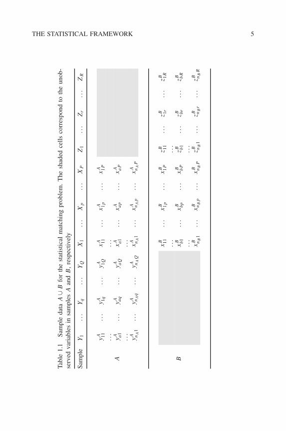
Table 1.1 shows typical statistical matching samples A and B. These samplescan be considered as a unique sample A ∪ B of nA + nB i.i.d. observations fromf (x, y, z) characterized by:

• the presence of missing data, and hence of a missing data generation mech-anism;

• the absence of joint information on X, Y, and Z.

The first point has been the focus of a very large statistical literature (see alsoAppendix A). The possible characterizations of the missing data generation mech-anisms for the statistical matching problem are treated in Section 1.3. It will beseen that standard inferential procedures for partially observed samples are alsoappropriate for the statistical matching problem.

The second issue is actually the essence of the statistical matching problem. Itstreatment is the focus throughout this book.

Remark 1.2 The previous framework for the statistical matching problem has fre-quently been used (at least implicitly) in practice. However, real statistical matchingapplications may not fit such a framework. One of the strongest assumptions is thatA ∪ B is a unique data set of i.i.d. records from f (x, y, z). When, for instance, thetwo samples are drawn at different times, this assumption may no longer hold.

Without loss of generality, let A be the most up-to-date sample of size nA stillfrom f (x, y, z) (which is the joint distribution of interest), with Z missing. Let B

be a sample independent of A whose nB sample units are i.i.d. from the distributiong(X, Y, Z), with g distinct from f . It is questionable whether these samples canbe statistically matched. Matching can actually be performed when, although thetwo distributions f and g differ, the conditional distribution of Z given X is thesame on both occasions. In this case, appropriate statistical matching procedureshave been defined which assign different roles to the two samples A and B: B

should lend information on Z to the A file. In the following it will be made clearwhenever this alternative framework is under consideration.

THE STATISTICAL FRAMEWORK 5

Tabl

e1.

1Sa

mpl

eda

taA

∪B

for

the

stat

istic

alm

atch

ing

prob

lem

.T

hesh

aded

cells

corr

espo

ndto

the

unob

-se

rved

vari

able

sin

sam

ples

Aan

dB

,re

spec

tivel

y

Sam

ple

Y1

...

Yq

...

YQ

X1

...

Xp

...

XP

Z1

...

Zr

...

ZR

yA 11

...

yA 1q

...

yA 1Q

xA 11

...

xA 1p

...

xA 1P

...

...

Ay

A a1

...

yA aq

...

yA aQ

xA a1

...

xA ap

...

xA aP

...

...

yA nA

1..

.y

A nAq

...

yA nA

Qx

A nA

1..

.x

A nAp

...

xA nAP

xB 11

...

xB 1p

...

xB 1P

zB 11

...

zB 1r

...

zB 1R

...

...

Bx

B b1

...

xB bp

...

xB bP

zB b

1..

.zB br

...

zB bR

...

...

xB nB

1..

.x

B nB

p..

.x

B nB

PzB nB

1..

.zB nB

r..

.zB nB

R

6 THE STATISTICAL MATCHING PROBLEM

1.3 The Missing Data Mechanism in the StatisticalMatching Problem

Before going into the details of the statistical matching procedures, let us describethe overall sample A ∪ B. As already described in Section 1.2, it is a sample ofnA + nB units from f (x, y, z) with Z missing in A and Y missing in B. Hence,the statistical matching problem can be regarded as a problem of analysis of apartially observed data set. Generally speaking, when missing items are present, itis necessary to take into account a set of additional r.v.s R = (

Rx, Ry, Rz

), where

Rx , Ry and Rz are respectively random vectors of dimension P , Q and R:

Rx = (RX1 , . . . , RXP

)′,

Ry = (RY1 , . . . , RYQ

)′,

Rz = (RZ1, . . . , RZR

)′.

The indicator r.v. RXjshows when Xj has been observed (RXj

= 1) or not(RXj

= 0), j = 1, . . . , P . Similar definitions hold for the random vectors Ry andRz. Appropriate inferences when missing items are present should consider a modelthat takes into account the variables of interest (X, Y, Z) and the missing data mech-anism R. Particularly important is the relationship among these variables, defined bythe conditional distribution of R given the variables of interest: h(rx, ry, rz|x, y, z).Rubin (1976) defines three different missing data models, which are generallyassumed by the analyst: missing completely at random (MCAR), missing at random(MAR), and missing not at random (MNAR); see Appendix A. Indeed, the statisti-cal matching problem has a particular property: missingness is induced by the sam-pling design. When A and B are jointly considered as a unique data set of nA + nB

independent units generated from the same distribution f (x, y, z), with Z missingin A and Y missing in B, i.e. for the statistical matching problem, the missing datamechanism is MCAR. A missing data mechanism is MCAR when R is independentof either the observed and the unobserved r.v.s X, Y and Z. Consequently,

h(rx, ry, rz|x, y, z) = h(rx, ry, rz). (1.1)

In order to show this assertion, it is enough to consider that R is independentof (X, Y, Z), i.e. equation (1.1), or, equivalently for the symmetry of the conceptof independence between r.v.s, that the conditional distribution of (X, Y, Z) givenR, say φ(x, y, z|rx, ry, rz) does not depend on R:

φ(x, y, z|rx, ry, rz) = φ(x, y, z),

for every x ∈ X , y ∈ Y , z ∈ Z .As a matter of fact, the statistical matching problem is characterized by just

two patterns of R:

THE MISSING DATA MECHANISM 7

• R = (111P ,111Q,000R) for the units in A and

• R = (111P ,000Q,111R

)for the units in B,

where 111j and 000j are two j -dimensional vectors of ones and zeros, respectively.Due to the i.i.d. assumption of the generation of the nA + nB values for (X, Y, Z),we have that

φ(x, y, z|111P ,111Q,000R

) = φ(x, y, z|111P ,000Q,111R

) = f (x, y, z) (1.2)

for every x ∈ X , y ∈ Y , z ∈ Z , where φ(x, y, z|111P ,111Q,000R

)is the distribution

which generates the records in sample A and φ(x, y, z|111P ,000Q,111R

)is the distri-

bution which generates the records in sample B. In other words, the missing datamechanism is independent of both observed and missing values of the variablesunder study, which is the definition of the MCAR mechanism. This fact allows thepossibility of making inference on the overall joint distribution of (X, Y, Z) withoutconsidering (i.e. ignoring) the random indicators R. Additionally, inferences canbe based on the observed sampling distribution. This is obtained by marginalizingthe overall distribution f (x, y, z) with respect to the unobserved variables. As aconsequence, the observed sampling distribution for the nA + nB units is easilycomputed:

nA∏

a=1

fXY (xa, ya)

nB∏

b=1

fXZ (xb, zb) . (1.3)

The observed sampling distribution (1.3) is the reference distribution for this book,as it is for most papers on statistical matching; see, for instance, Rassler (2002,pg. 78). The following remark underlines which alternatives can be considered,what missing data generation mechanism refers to them, and their feasibility.

Remark 1.3 Remark 1.2 states that A and B cannot always be considered as gen-erated from an identical distribution. In this case, equation (1.1) no longer holds andthe missing data mechanism in A ∪ B cannot be assumed MCAR. In the notationof Remark 1.2, the distributions of (X, Y, Z) given the patterns of missing data are:

φ(x, y, z|111P ,111Q,000R

) = f (x, y, z) ,

φ(x, y, z|111P ,000Q,111R

) = g (x, y, z) ,

for every x ∈ X , y ∈ Y , z ∈ Z . This situation can be formalized via the so-calledpattern mixture models (Little, 1993): if the two samples are analysed as a uniquesample of nA + nB units, the corresponding generating model is a mixture of thetwo distributions f and g. Little warns that this approach usually leads to underi-dentified models, and shows which restrictions that tie unidentified parameters withthe identified ones should be used. In general, as already underlined in Remark 1.2,the interest is not in the mixture of the two distributions, but only in the most up-to-date one, f (x, y, z) (an exception will be illustrated in Remark 6.1). For thisreason, these models will not be considered any more. The framework illustratedin Remark 1.2 will just consider B as a donor of information on Z, when possible.

8 THE STATISTICAL MATCHING PROBLEM

1.4 Accuracy of a Statistical Matching Procedure

Sections 1.2 and 1.3 have described the input of the statistical matching problem:a partially observed data set with the absence of joint information on the variablesof interest and some basic assumptions on the data generating model. This sectiondeals with the output. As declared in Section 1.1, the statistical matching problemmay be addressed using either the micro or macro approach. These approaches canbe adopted by using many different statistical procedures, i.e. different transforma-tions of the available (observed) data. Are there any guidelines as to the choice ofprocedure? In other words, how is it possible to assess the accuracy of a statisticalmatching procedure?

It must be remarked that it is not easy to draw definitive conclusions. Papersthat deal explicitly with this problem are few in number, among them Barr andTurner (1990); see also D’Orazio et al. (2002) and references therein. A numberof different issues should be taken into account.

(a) What assumptions can be reasonably considered for the joint model (X, Y, Z)?

(b) What estimator for f (x, y, z) is preferable, if any, under the model assumedin (a)?

(c) What method of generating appropriate values for the missing variables canbe used under the model chosen in (a) and according to the estimator chosenin (b)?

As a matter of fact, (a) is a very general question related to the data generationprocess, (b) is related to the macro approach, and (c) to the micro approach. Theyare interrelated in the sense that an apparently reasonable answer to a questionis not reasonable if the previous questions are unanswered. Actually, there is yetanother question that should be considered when a synthetic file is distributed andinferential methods are applied to it.

(d) What inferential procedure can be used on the synthetic data set?

The combination of (a) and (b) for the macro approach, (a), (b) and (c) for themicro approach, and (a), (b), (c), and (d) for the analysis of the result of the microapproach gives an overall sketch of the accuracy of the corresponding statisticalmatching result. A general measure that amalgamates all these aspects has not beenyet defined. It can only be assessed via appropriate Monte Carlo experiments in asimulated framework.

Let us investigate each of the accuracy issues (a)–(d) in more detail.

1.4.1 Model assumptions

Table 1.1 shows that the statistical matching problem is characterized by a veryannoying situation: there is no observation where all the variables of interest are

ACCURACY OF A STATISTICAL MATCHING PROCEDURE 9

jointly recorded. A consequence is that, of all the possible statistical models for(X, Y, Z), only a few are actually identifiable for A ∪ B. In other words, A ∪ B

does not contain enough information for the estimation of parameters such as thecorrelation matrix or the contingency table of (Y, Z). Furthermore, for the samereason, it is not possible to test on A ∪ B which model is appropriate for (X, Y, Z).There are different possibilities.

• Further information (e.g. previous experience or an ad hoc survey) justifiesthe use of an identifiable model for A ∪ B.

• Further information (e.g. previous experience or an ad hoc survey) is usedtogether with A ∪ B in order to make other models also identifiable.

• No assumptions are made on the (X, Y, Z) model. This problem is studiedas a problem characterized by uncertainty on some of the model properties.

The first two assumptions are able to produce a unique point estimate of the param-eters. For the third choice, which is a conservative one, a set rather than a pointestimate of the inestimable parameters, such as the correlation matrix of (Y, Z),will be the output. The features of this set of estimates describe uncertainty forthat parameter.

The first two choices are assumptions that should be well justified by additionalsources of information. If these assumptions are wrong, no matter what sophisti-cated inferential machinery is used, the results of the macro and, hence, of themicro approaches will reflect the assumption and not the real underlying model.Also in these cases, evaluation of uncertainty is a precious source of information.In fact, reliability of conclusions based on one of the first two choices can bebased on the evaluation of their uncertainty when no assumptions are considered.For instance, if a correlation coefficient for the never jointly observed variables Yand Z is estimated under a specific identifiable model for A ∪ B or with the helpof further auxiliary information, an indication of the reliability of these estimatesis given by the width of the uncertainty set: the smaller it is, the higher is thereliability of the estimates with respect to model misspecification.

1.4.2 Accuracy of the estimator

Let us assume that a model for (X, Y, Z) has been firmly established. When theapproach is macro, accuracy of a statistical matching procedure means accuracy ofthe estimator of the distribution function f (x, y, z). In this case, appropriate mea-sures such as the mean square error (MSE) or, accounting for its components, thebias and variance are well known in both the parametric and nonparametric case.

In a parametric framework, minimization of the MSE of each parameter estima-tor can (almost) be obtained, at least for large data sets and under minimal regularityconditions, when maximum likelihood (ML) estimators are used. More precisely,the consistency property of ML estimators is claimed in most of the results of thisbook. It must be emphasized that the ML approach given the overall set A ∪ B

10 THE STATISTICAL MATCHING PROBLEM

has an additional property in this case: every parameter estimate is coherent withthe other estimates. Sometimes a partially observed data set may suggest distinctestimators for each parameter of the joint distribution that are not coherent. It willbe seen that this issue is fundamental in statistical matching, given that it dealswith the partially observed data set of Table 1.1.

In a nonparametric framework, consistency of the results is also one of themost important aspects to consider. Consistency of estimators is a very importantcharacterization for the statistical matching problem. In fact, it ensures that, for largesamples, estimates are very close to the true but unknown distribution f (x, y, z).In the next subsection it will be seen that this aspect is relevant also to the microapproach.

1.4.3 Representativeness of the synthetic file

This aspect is the most commonly investigated issue for assessing the accuracyof a statistical matching procedure. Generally speaking, four large categories ofaccuracy evaluation procedures can be defined (Rassler, 2002), from the mostdifficult goal to the simplest:

(i) Synthetic records should coincide with the true (but unobserved) values.

(ii) The joint distribution of all variables is reflected in the statistically matchedfile.

(iii) The correlation structure of the variables is preserved.

(iv) The marginal and joint distributions of the variables in the source files arepreserved in the matched file.

The first point is the most ambitious and difficult requirement to fulfil. It can beachieved when logical or mathematical rules determining a single value for-eachsingle unit are available. However, when using statistical rules, it is not as importantto reproduce the exact value as it is the joint distribution f (x, y, z), which containsall the relevant statistical information.

The third and fourth points do not ensure that the final synthetic data set isappropriate for any kind of inferences for (X, Y, Z), contradicting one of the maincharacteristics that a synthetic data set should possess. For instance, the fourthpoint ensures only reasonable inferences for the distributions of (X, Y) and (X, Z).

When the second goal is fulfilled, the synthetic data set can be considered as asample generated from the joint distribution of (X, Y, Z). Hence, the synthetic dataset is representative of f (x, y, z), and can be used as a general purpose sample inorder to infer its characteristics.

Any discrepancy between the real data generating model and the underlyingmodel of the synthetic complete data set is called matching noise; see Paass (1985).

Focusing on the second point, under identifiable models or with the help ofadditional information (Section 1.4.1), the relevant question is whether the data

OUTLINE OF THE BOOK 11

synthetically generated via the estimated distribution f (x, y, z) are affected by thematching noise or not. It is not always a simple matter. As claimed in Section 1.4.2,when the available data sets are large and the macro approach is used with aconsistent estimator of f (x, y, z), it is possible to define micro approaches with areduced matching noise. Note that a good estimate of f (x, y, z) is a necessary butnot a sufficient condition to ensure that the matching noise is as low as possible.In fact, the generation of the synthetic data should be also done appropriately.

1.4.4 Accuracy of estimators applied on the synthetic data set

This is a critical issue for the micro approach. If the synthetic data set can beconsidered as a sample generated according to f (x, y, z) (or approximately so),it is appropriate to use estimators that would be applied in complete data cases.Hence, the objective of reducing the matching noise (Section 1.4.3) is fundamental.

In fact, estimators preserve their inferential properties (e.g. unbiasedness, con-sistency) with respect to the model that has generated the synthetic data. Whenthe matching noise is large, these results are a misleading indication as to the truemodel f (x, y, z).

As a matter of fact, this last problem resembles that of Section 1.4.1. InSection 1.4.1 there was a model misspecification problem. Now the problem isthat the data generating model of the synthetic data set differs from the data gener-ating model of the observed data set. In both cases the result is similar: inferencesare related to models that differ from the target one.

1.5 Outline of the Book

This book aims to explore the statistical matching problem and its possible solu-tions. This task will be addressed by considering features of its input (Sections 1.2and 1.3) and, more importantly, of its output (Section 1.4).

One of the key issues is model assumption. As remarked in Section 1.4.1, a firstset of techniques refer to the case where the overall model family F is identifiablefor A ∪ B. A natural identifiable model is one that assumes the independence ofY and Z given X. This assumption is usually called the conditional independenceassumption (CIA). Chapter 2 is devoted to the description and analysis of thedifferent statistical matching approaches under the CIA.

The set of identifiable models for A ∪ B is rather narrow, and may be inappro-priate for the phenomena under study. In order to overcome this problem, furtherauxiliary information beyond just A ∪ B is needed. This auxiliary information maybe either in parametric form, i.e. knowledge of the values of some of the param-eters of the model for (X, Y, Z), or as an additional data sample C. The use ofauxiliary information in the statistical matching process is described in Chapter 3.

Both Chapters 2 and 3 will consider the following aspects:

(i) macro and micro approaches;

12 THE STATISTICAL MATCHING PROBLEM

(ii) parametric and nonparametric definition of the set of possible distributionfunctions F ;

(iii) the possibility of departures from the i.i.d. case (as in Remark 1.2).

As claimed in Section 1.4.1, a very important issue deals with the situation whereno model assumptions are hypothesized. In this case, it is possible to study theuncertainty associated to the parameters due to lack of sample information. Giventhe importance of this topic, it is described in considerable detail in Chapter 4.

The framework developed in Section 1.2 is not the most appropriate for samplesdrawn from finite populations according to complex survey designs, unless ignor-ability of the sample design is claimed; see, for example, Gelman et al. (2004,Chapter 7). Despite the amount of data sets of this kind, only few methodologicalresults for statistical matching are available. A general review of these approachesand the link with the corresponding results under the framework of Section 1.2 isgiven in Chapter 5.

Generally speaking, statistical integration of different sources is strictly con-nected to the integration of the data production processes. Actually, statisticalintegration of sources would be particularly successful when applied to sourcesalready standardized in terms of definitions and concepts. Unfortunately, this isnot always true. Some considerations on the preliminary operations needed forstatistically matching two samples are reported in Chapter 6.

Finally, Chapter 7 presents some statistical matching applications. A particularstatistical matching application is described in some detail in order to make clear allthe tasks that should be considered when matching two real data sets. Furthermore,this example allows the comparison of the results of different statistical matchingprocedures.

All the original codes used for simulations and experiments, developed in theR environment (R Development Core Team, 2004), are reported in Appendix E inorder to enable the reader to make practical use of the techniques discussed in thebook. The same codes can also be downloaded on the site http://www.wiley.com/go/matching.