Statistical Inference

• Statistical Inference is the process of making judgments about a population based on properties of the sample• intuition only goes so far towards making

decisions of this nature • experts can offer conflicting opinions using

the same data

Methods of Statistical Inference

• Estimation• Predict the value of an unknown parameter

with specified confidence

• Decision Making• Decide between opposing statements about

the population (parameter)

Estimation

• Estimating a Population Mean (m)• Point Estimate

• Mean, median, mode, etc.• Easy to calculate and use, but random in value

• Interval Estimate• Range of values containing parameter• Unknown accuracy within range

• Confidence Interval• Interval with known probability of containing truth• Often based on a “pivot statistic” with known

distribution

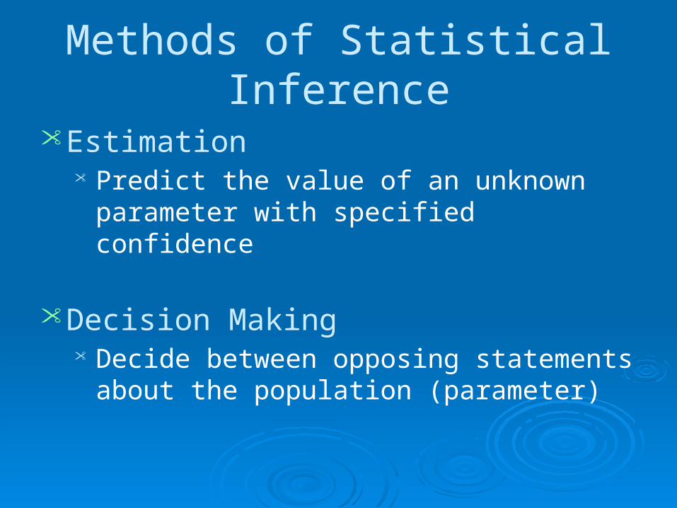
Estimating ( m s known)• The central limit theorem provides a sampling

distribution for the sample mean in cases of sufficient sample size (n ≥ 30). The following probability statement can be used to find a confidence interval for μ:

/ 2 / 2

/ 2 / 2

1 ( )

( )

P z Z zx

P z z

n

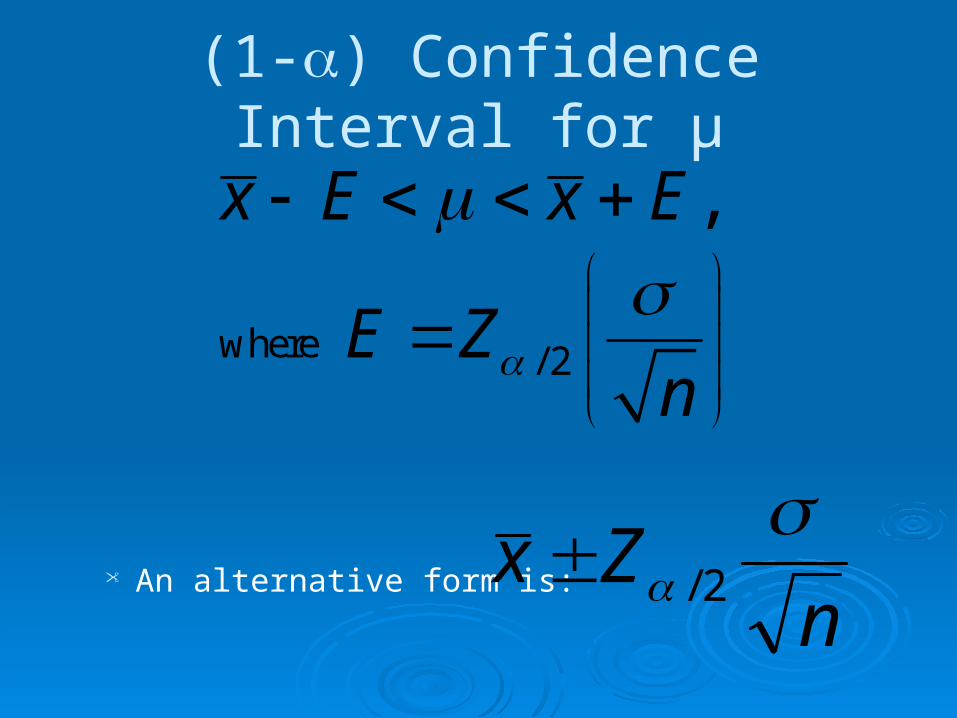
(1-a) Confidence Interval for μ

• An alternative form is:

nZx

2/

where / 2

, x E x E

E Zn

Confidence Intervals

• The level of confidence and sample size both effect the width of the confidence interval. • Increasing the level of confidence results in a wider

confidence interval. • Increasing the sample size results in a narrower

confidence interval. • Setting the level of confidence too high results in a

confidence interval that is too wide to be of any practical use. • i.e. 100% confidence intervals are from -∞ to ∞

Bootstrap Confidence Intervals

• The bootstrap technique can be used to obtain a confidence interval estimate.• Simulate 1000 bootstrap samples from the data.• The 25th order statistic and the 975th order statistic are

used as the lower and upper bounds, respectively.• This is a non-parametric approach since no

assumptions are made about the underlying distribution of the data.

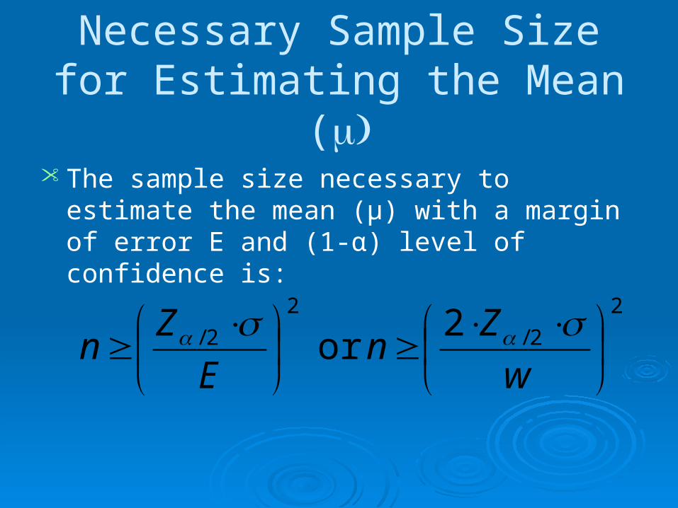
Necessary Sample Size for Estimating the Mean ( )m

• The sample size necessary to estimate the mean (μ) with a margin of error E and (1-α) level of confidence is:

2

2/

2

2/ 2or

w

Zn

E

Zn

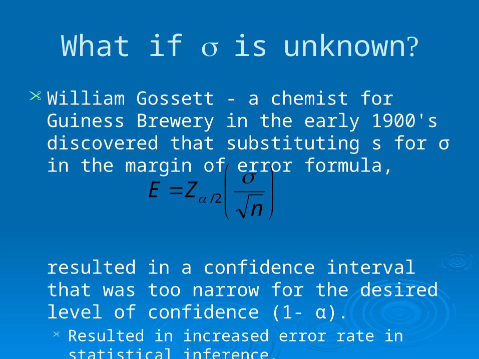
What if s is unknown?• William Gossett - a chemist for Guiness Brewery

in the early 1900's discovered that substituting s for σ in the margin of error formula,

resulted in a confidence interval that was too narrow for the desired level of confidence (1- α). • Resulted in increased error rate in statistical inference. • Error rate particularly noticeable for small samples

n

ZE

2/

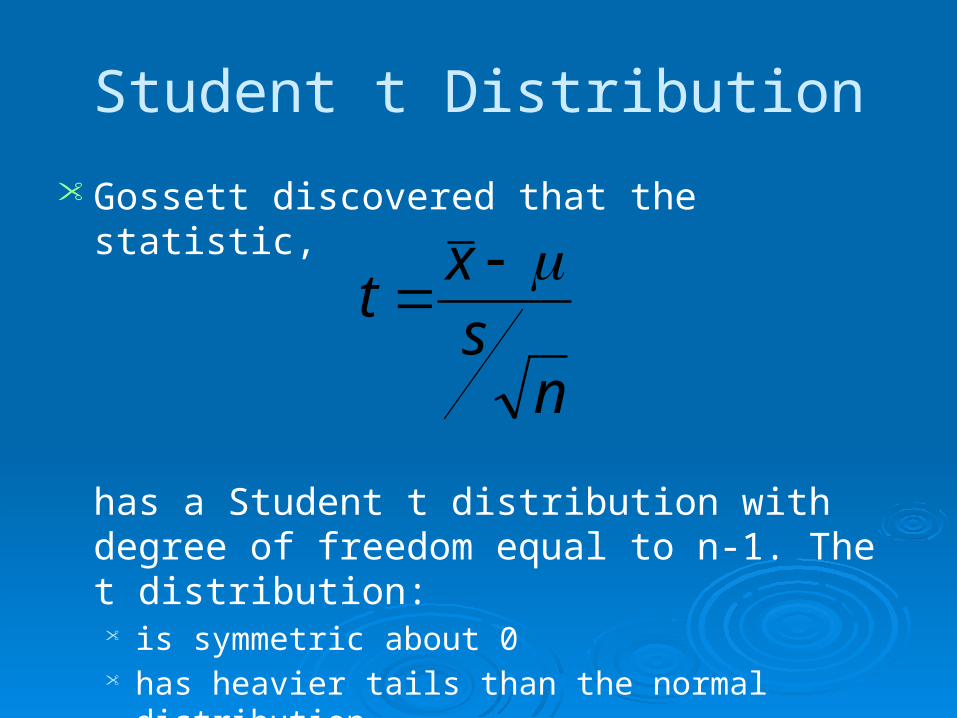
Student t Distribution

• Gossett discovered that the statistic,

has a Student t distribution with degree of freedom equal to n-1. The t distribution: • is symmetric about 0• has heavier tails than the normal distribution• converges to the normal distribution as n∞.

nsx

t

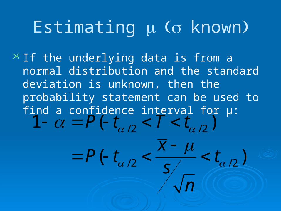
Estimating ( m s known)• If the underlying data is from a normal distribution

and the standard deviation is unknown, then the probability statement can be used to find a confidence interval for μ:

/ 2 / 2

/ 2 / 2

1 ( )

( )

P t T tx

P t tsn

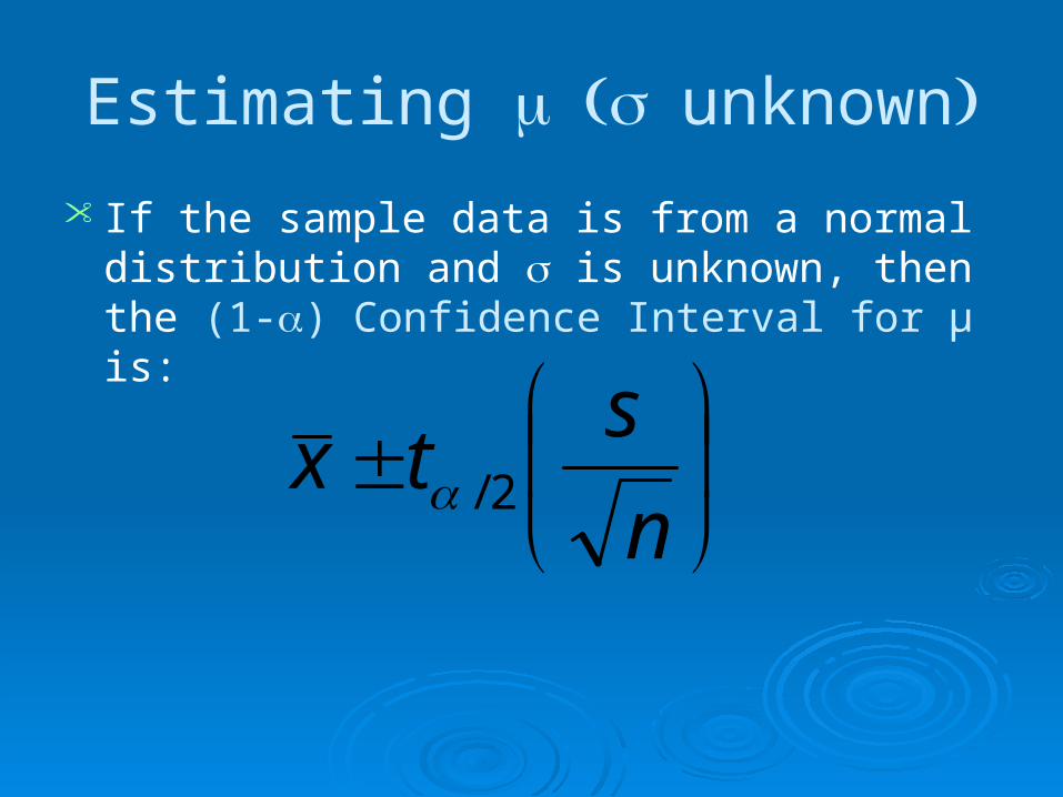
Estimating ( m s unknown)• If the sample data is from a normal distribution

and s is unknown, then the (1-a) Confidence Interval for μ is:

n

stx 2/

Why settle for small sample size?

• Can’t you just collect more data?• Samples can be expensive to obtain.

• shuttle launch, batch run• Samples can be difficult to obtain.

• rare specimen, chemical process• Samples can be time consuming to obtain.

• cancer research, effects of time• Ethical questions can arise.

• medical research can't continue if initial results look bad

Estimating Population Proportion (p)

• Can be thought of as the binomial probability of success if randomly sampling from the population. • Let p be the proportion of the population with some

characteristic of interest. The characteristic is either present or it is not present, so the number with the characteristic is binomial.

Estimating Population Proportion (p)

• The central limit theorem applies to a binomial random variable with sufficient sample size• Expected number of successes (n·p) and failures (n·q)

must be at least 5. • The number of successes (X) is normally

distributed with mean n·p and variance n·p·q. • The proportion of interest is normally

distributed, with mean p and variance of p·q/n.

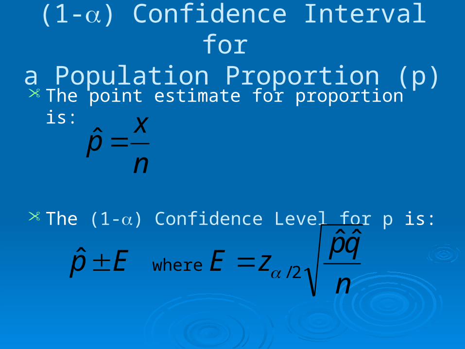
(1-a) Confidence Interval for a Population Proportion (p)

• The point estimate for proportion is:

• The (1-a) Confidence Level for p is:

n

qpzEEp

ˆˆ ˆ 2/ where

n

xp ˆ

Necessary Sample Size for Estimating the Proportion (p)

• The sample size necessary to estimate the proportion (p) a margin of error E and (1-a) level of confidence (a) with prior knowledge of p and q and (b) no prior knowledge of p and q is.

2

2/

2 )

E

Znb **

2

2/ ) qpE

Zna

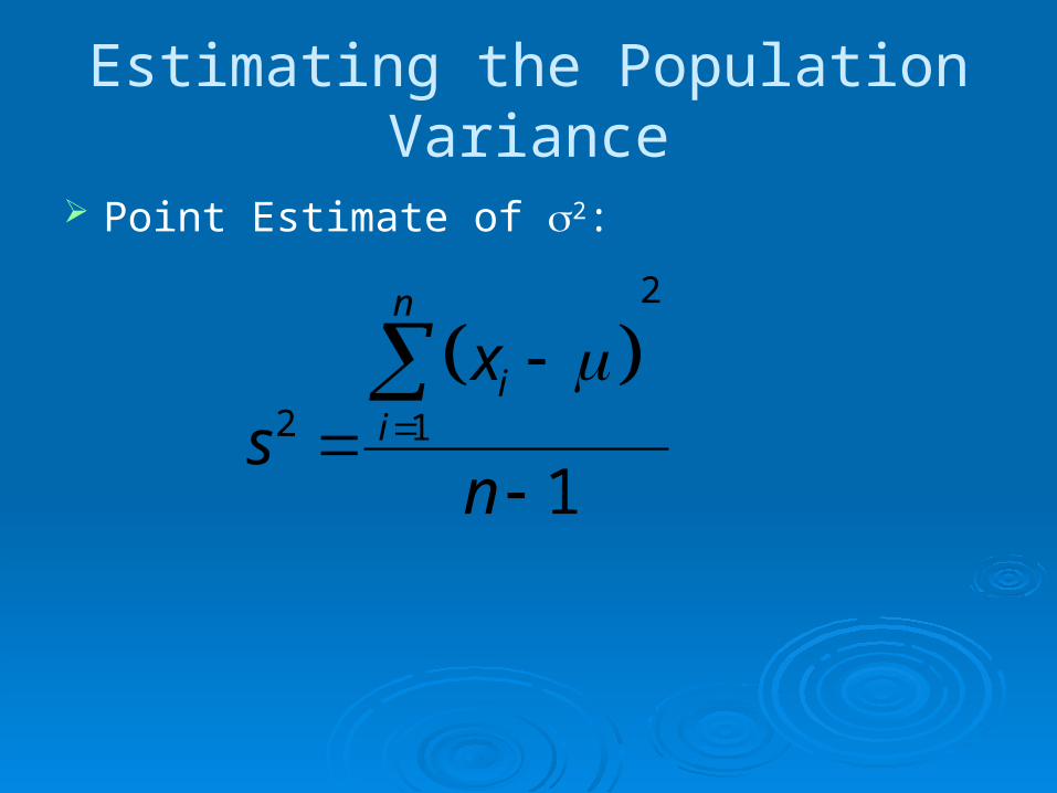
Estimating the Population Variance

Point Estimate of s2:

2

2 1

1

n

ii

xs

n

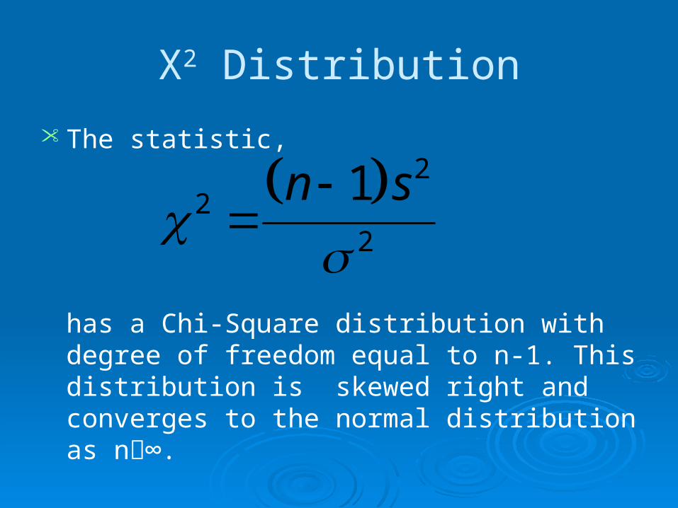
Χ2 Distribution

• The statistic,

has a Chi-Square distribution with degree of freedom equal to n-1. This distribution is skewed right and converges to the normal distribution as n∞.

22

2

1n s

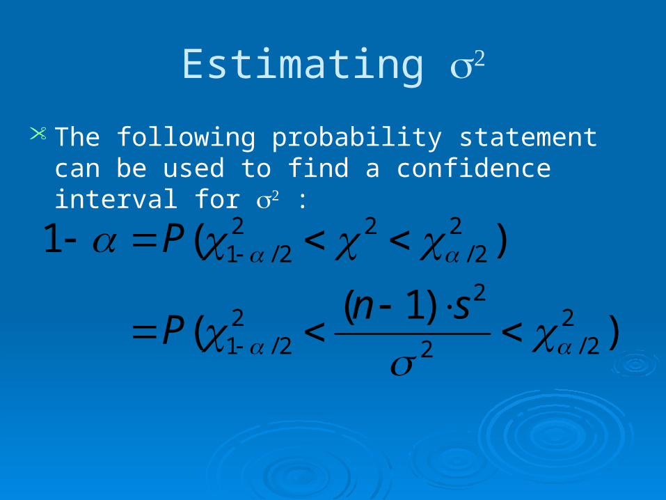
Estimating s2

• The following probability statement can be used to find a confidence interval for s2 :

))1(

(

)(1

22/2

22

2/1

22/

222/1

snP

P

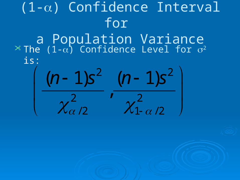
(1-a) Confidence Interval for a Population Variance

• The (1-a) Confidence Level for s2 is:

2 2

2 2/ 2 1 / 2

( 1) ( 1),

n s n s