Statistical Hypotheses Testing Stat 700 Lectures Hypothesis Testing

Statistical Hypotheses Testing

Stat 700 Lectures

Hypothesis Testing

Week of 11/06/200 Hypotheses Testing 2

Overview of this Lecture The problem of hypotheses testing Elements and logic of hypotheses testing

(hypotheses, decision rule, one- and two-tailed tests, significance level, Type I and Type II errors, power of test, implications of the decision, p-values)

Steps in performing a hypotheses test Large-sample test for the population mean Two-sample tests for the population means Large-sample test for the population proportion Two-sample tests for the population proportions


The problem of hypotheses testing Statement of the Problem: Given a population (equivalently a distribution) with a

parameter of interest, , (which could be the mean, variance, standard deviation, proportion, etc.), we would like to decide/choose between two complementary statements concerning . These statements are called statistical hypotheses.

The choice or decision between these hypotheses is to be based on a sample data taken from the population of interest.

The ideal goal is to be able to choose the hypothesis that is true in reality based on the sample data.


Some Situations where Hypotheses Testing is Relevant Example: A drug manufacturer would like to compare

a newly developed pill for eliminating migraine headaches relative to a standard drug. Such a comparison is to be done by comparing the mean time to cessation of headache after taking the pill. Let denote the mean time to headache cessation after taking the new pill. If 0 is the mean time to headache cessation for the standard drug, then the manufacturer would like to decide between:

Statement 1 (Null): > 0 (new drug is not better)

Statement 2 (Alternative): < 0 (new drug is better)


Some Situations … Example: A medical researcher would like to

compare the effectiveness of two treatments (for example, chemotherapy versus radiation-based) for a particular type of cancer, with the effectiveness being measured in terms of the five-year survival rate of patients. If p1 denotes the proportion of patients surviving 5 years which were treated with chemotherapy, and p2 is the survival proportion for those treated with radiation, then the researcher would like to decide between:

Statement 1: p1 < p2;

Statement 2: p1 > p2.


Some Situations ... Example: The Food and Drug Administration would

like to check that the amount of an active ingredient of a certain substance in a certain type of medication is as specified in the label. If is the mean amount of this substance, then the FDA would like to decide between the statements:

Statement 1 (Null): = 0, where 0 is the specified amount;

Statement 2 (Alternative): 0.

This is an example of a two-sided hypothesis since it indicates that either < 0 or > 0.


Elements and Logic of Statistical Hypotheses Testing

Consider a population or distribution whose mean is . To introduce the elements and discuss the logic of hypotheses testing, we consider the problem of deciding whether = 0, where 0 is a pre-specified value, or 0. This is the type of problem that the FDA might be interested.

The first step in hypotheses testing, which should be done before you gather your sample data, is to set up your statistical hypotheses, which are the null hypothesis (H0) and the alternative hypothesis (H1).


The Statistical Hypotheses The null hypothesis, H0, is usually the hypothesis that

corresponds to the status quo, the standard, the desired level/amount, or it represents the statement of “no difference.”

The alternative hypothesis, H1, on the other hand, is the complement of H0, and is typically the statement that the researcher would like to prove or verify.

These hypotheses are usually set-up in such a way that deciding in favor of H1 when in fact H0 is the true statement will not be a desirable outcome.


An Analogy to Remember

Setting the null and alternative hypotheses has an analog in the justice system where the defendant is “presumed innocent” until “proven guilty.”

In the court system, the null hypothesis corresponds to the defendant being innocent (this is the status quo, the standard, etc.).

The alternative hypothesis, on the other hand, is that the defendant is guilty.

Note that it is very difficult to reject the null (convict the defendant), and only “a proof (based on good evidence) beyond a reasonable doubt” will warrant rejection of H0.


The Hypotheses in our Problem For the problem we are considering, the appropriate

hypotheses will be:

H0: = 0

H1: 0.

Another word of caution: It is not proper for a researcher to set up the hypotheses after seeing the sample data; however, a data maybe used to generate a hypotheses, but to test these generated hypotheses you should gather a new set of sample data!


Determine the Type of Sample Data that will be Gathered

The second step is to determine what kind of sample data you will be gathering. Is it a simple random sample? A stratified sample?

For the moment we will assume that a simple random sample of size n will be obtained, so the data will be representable by X1, X2, …, Xn, with n > 30.

Also, determine if you know the population standard deviation . We assume for the moment that we do.


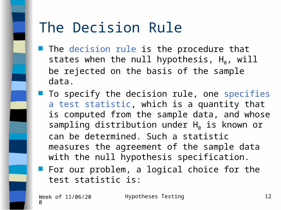
The Decision Rule The decision rule is the procedure that states when

the null hypothesis, H0, will be rejected on the basis of the sample data.

To specify the decision rule, one specifies a test statistic, which is a quantity that is computed from the sample data, and whose sampling distribution under H0 is known or can be determined. Such a statistic measures the agreement of the sample data with the null hypothesis specification.

For our problem, a logical choice for the test statistic is:


The Test Statistic:

The latter is a reasonable choice since it measures how far the sample mean is from the population mean under H0. The larger the value of |Zc| the more it will indicate that H0 is not true.

Furthermore, under H0, by virtue of the Central Limit Theorem, the sampling distribution of Zc will be approximately standard normal.

. ly,equivalentor 0

n

XZX c


When to Reject H0 and its Consequences

Having decided which test statistic to use, the next step is to specify the precise situation in which to reject H0. We have said that it is logical to reject H0 if the absolute value of Zc is large.

But how “large” is “large”? For the moment, let us specify a critical value,

denoted by C, such that if |Zc| > C

then H0 will be rejected. Before deciding on the value of C, let us examine the

consequences of our decision rule.


Possible Errors of Decision

Remember at this stage that either H0 is correct, or H1 is correct. Thus, there is a “true state of reality,” but this state is not known to us (otherwise we wouldn’t be performing a test).

On the other hand, our decision on whether to reject H0 will only be based on partial information, which is the sample data.

We may therefore represent in a table the possible combinations of “states of reality” and “decision based on the sample” as follows:


States of Reality and Decisions Made

In decision-making, there is therefore the possibility of committing an error, which could either be an error of Type I or an error of Type II.

Which of these two types of error is more serious??

State of RealityH0 True H0 False

Do not rejectH0

CorrectDecision

Error inDecision

(Type II error)

DecisionMade Basedon Sample

DataAccording to

Rule

Reject H0 Error inDecision

(Type I error)

CorrectDecision


Assessing the Two Types of Errors

From the table in the preceding slide, we have: Type I error: committed when H0 is rejected when in

reality it is true. Type II error: committed when H0 is not rejected

when in reality it is false.

Just like in the court trial alluded to earlier, an error of Type I is considered to be a more serious type of error (“convicting an innocent man”).

Therefore, we try to minimize the probability of committing the Type I error.


Setting the Probability of a Type I Error

In trying to minimize, however, the probability of a Type I error, we encounter an obstacle in that the probabilities of the Type I and Type II errors are inversely related. Thus, if we try to make the probability of a Type I error very, very small, then it will make the probability of a Type II error quite large.

As a compromise we therefore specify a maximum tolerable Type I error probability, called the significance level, and denoted by , and choose the critical value C such that the probability of a Type I error is (at most) equal to .

This is conventionally set to 0.10, 0.05, or 0.01.


Determining the Critical Value, C Let us now determine the critical value C in our test.

Recall that our test will reject H0 if |Zc| > C. By definition, P{Type I error} = P{reject H0 | H0 is true} = P{|Zc| > C |

H0 is true}.

But, under H0, Zc is distributed as standard normal, so if we want P{Type I error} = , then we should choose the critical value C to be:

C = Z/2, which is the value such that P{Z > Z/2} = /2.


The Resulting Decision Rule

Given a significance level of , for testing the null hypothesis H0: = 0 versus the alternative hypothesis H1: 0, the appropriate test statistic, under the assumptions that (a) is known, and (b) n > 30 is given by:

. if HReject 2

00

z

n

XZc


Data Gathering and Making the Decision

Having specified the final decision rule, the next step is to gather the sample data and to compute the sample mean and the value of Zc.

If |Zc| > z/2 then H0 is rejected; otherwise, we say that we “fail to reject H0.”

Note: If is not known, then we could replace it in the formula of Zc by the sample standard deviation S.

The final step is to make the relevant conclusion.


On the Conclusion that One Could Make

The final step in performing a statistical test of hypotheses is to make the conclusion relevant to the particular study, that is, not to simply say that “H0 is rejected” or “H0 is not rejected.”

When H0 is rejected, then either that a correct decision has been made, or an error of Type I has been committed. But since we have controlled the probability of committing a Type I error (set to , which we could tolerate), then we can conclude in this case that H0 is not true, and hence that H1 is correct.


On Conclusions … continued On the other hand, if we did not reject H0, then either

we are making the correct decision, or we are making a Type II error.

However, since we did not control for the Type II error probability (when we set the Type I error probability to be , we “closed our eyes to the probability of a Type II error”), if we do not reject H0, we cannot conclude that H0 is true. Rather, we could only say that we “failed to reject H0 on the basis of the available data.”

This is the basis of the saying that: “you can never prove a theory, you can only disprove it.”


Recapitulation: Steps in Hypotheses Testing

Step 1: Formulate your null and alternative hypotheses.

Step 2: Determine the type of sample you will be getting with regards to sample size, knowledge of the standard deviation, etc.

Step 3: Specify your level of significance. Step 4: State precisely your decision rule. Step 5: Gather your sample data and compute the

test statistic. Step 6: Decide and make final conclusions.


The p-Value Approach Another approach to making the decision in

hypotheses testing is to compute the p-value associated with the observed value of the test statistic.

By definition, the p-value is the probability of getting the observed value or more extreme values of the test statistic under H0.

In our situation, the p-value would then be: p-value = P{|Z| > |zc|} where zc is the observed value of

the test statistic.


Deciding Based on the p-Value

If the p-value exceed 0.10, then H0 is not rejected and we say that the result is not significant.

If the p-value is between 0.10 and 0.05, we usually say that the result is almost significant or tending towards significance.

If the p-value is between 0.05 and 0.01, we reject H0 and conclude that the result is significant.

If the p-value is less than 0.01 then H0 is rejected and conclude that the result is highly significant.


On the Sensitivity of a Test Ideally, we would like our test procedure to always

produce the correct decision. However, this is not possible if the decision is based only on sample data.

To measure the sensitivity of a test under the alternative hypothesis, we can compute its power, which is the probability of rejecting H0 under the alternative hypothesis.

That is, Power of Test at 1 = P{reject H0 | = 1}. This function could be plotted and can be used to determine the appropriate sample size.


Some Concrete Problems Situation: The mean yield of corn in the US is about

120 bushels per acre. A survey of 40 farmers this year gives a sample mean yield of 123.8 bushels per acre. We want to know whether this is good evidence that the national mean this year is not 120 bushels per acre. Assume that the farmers surveyed are an SRS from the population of all commercial corn growers and that the standard deviation of the yield in this population is = 10 bushels per acre. Test H0: = 120 versus H1: 120 at 5% level of significance.

Solution: Because H1 is a two-sided hypothesis and


Solution … continued Level of significance is = 0.05, then the appropriate

decision rule is: Reject H0 if |Zc| > z.025 = 1.96, where the test statistic is

Zc = (Xbar -0)/(/n1/2). From the given information, the value of this test

statistic is Zc = (123.8 - 120)/[10/401/2] = 2.4033. Since this value is larger than the critical value of 1.96,

then our decision is to reject H0 at 5% significance level.

We can therefore conclude at the 5% level that the mean yield of corn for this year is different from the usual mean yield of 120 bushels per acre.


P-value Approach Illustrated Recall that the p-value is the probability, under H0, of

getting the observed value of the test statistic or more extreme values. For our problem, we therefore have:

p-value = P{|Z| > 2.4033} = 0.0162. Based on this value we could reject H0 at the 5%

level, but not at the 1% level. Another interpretation of the p-value of 0.0162 is that

it is the smallest level of significance at which H0 can be rejected.

Let us also examine the power of our test.


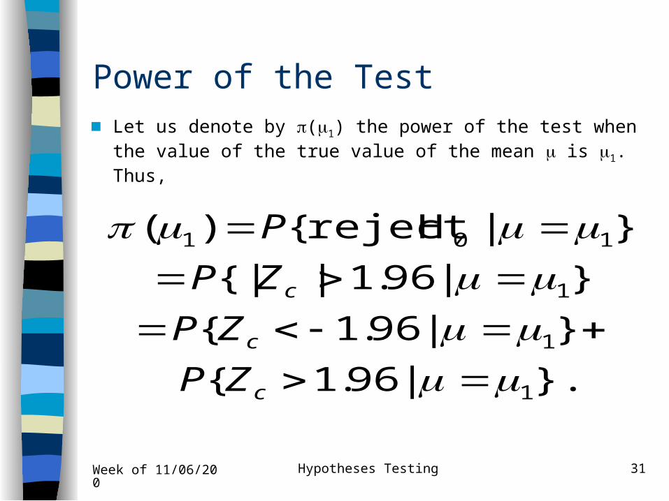
Power of the Test Let us denote by (1) the power of the test when the

value of the true value of the mean is 1. Thus,

}.|96.1{

}|96.1{

}|96.1|{|

}|Hreject {)(

1

1

1

101

c

c

c

ZP

ZP

ZP

P


Power … continued

.)(

96.1)(

96.1)(

Therefore,

when Since

01011

1.0010

nZP

nZP

n

Z

nn

X

n

XZc

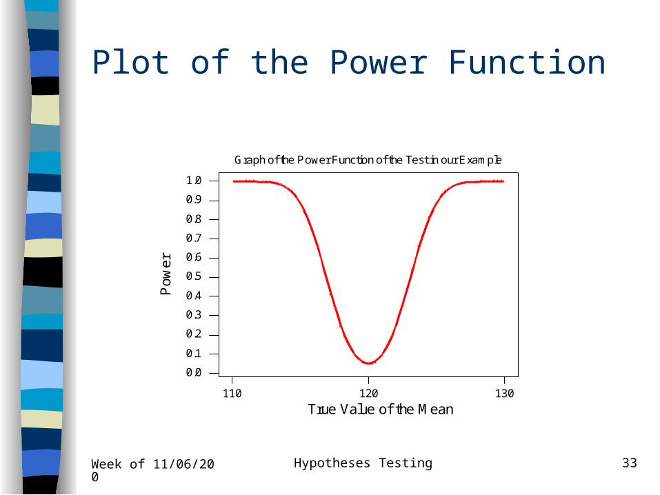
Substituting 0 = 120, = 10, and n = 40 into the above expression, we can then calculate the value of (1) for different values of 1.

The values of 1 and (1) could then be plotted. This plot is given in the next slide.


Plot of the Power Function

110 120 130

0.0

0.1

0.2

0.3

0.4

0.5

0.6

0.7

0.8

0.9

1.0

True Value of the Mean

Pow

erGraph of the Power Function of the Test in our Example


Problems ... Situation: The Survey of Study Habits and Attitudes

(SSHA) is a psychological test that measures the motivation, attitude toward school, and study habits of students. Scores range from 0 to 200. The mean score for US college students is about 115, and the standard deviation is about 30. A teacher who suspects that older students have better attitudes toward school gives the SSHA to 20 students who are at least 30 years of age. Their mean score is 135.2. Assume that = 30. Perform a test of H0: = 115 versus H1: > 115 using the p-value approach.

Solution: To be done in class.


Some Comments on Assumptions The testing procedure we developed here required

two assumptions: (a) sample size is at least 30; (b) population standard deviation is known. Assumption (b) is not crucial since could be

replaced by S in the formula for Zc. When assumption (a) is not satisfied, then we need

to be able to assume that the population is normal and we need to know the population standard deviation.

If is not known, we will need to use the t-distribution, which will be discussed next week.


Concrete Problems for Testing Two Means

Question of Interest: Does cocaine use by pregnant women cause their babies to have low birth weight?

Hypothesis:

– H0: Mean birth weight of babies of cocaine users is greater than or equal to the mean birth weight of babies from non-cocaine users. Symbolically, 1 > 2.

– H1: 1 < 2.


Data of the Study

Data Gathering Performed: Birth weights (measured in grams) of babies of women who tested positive for cocaine/crack during a drug-screening test were compared with the birth weights for women who either tested negative or were not tested, a group called “other.” Below is the summary statistics for the two samples.

Group Sample Size Sample Means SampleStandardDeviation

Positive Test 134 2733 599Other 5974 3118 672


Problems … continued

Study Question: Is the mean hemoglobin level among breast-fed babies higher than those fed with standard baby formula without iron supplements?

What are the appropriate hypotheses?

Situation: A study of iron deficiency among infants compared the samples of infants following different feeding regimens. One group contained breast-fed infants, while the children in another group were fed a standard baby formula without any iron supplements. A summary of the blood hemoglobin levels at 12 months of age is presented in the following table.


Summary of the Data from Study

The appropriate test will be done in class. What conclusions could be made? What assumptions are needed for the test to be

valid? What if the standard deviations that were provided

were actually the sample standard deviations?

Group Sample Size Sample Means PopulationStandardDeviation

Breast-Fed 23 13.3 1.7Formula 19 12.4 1.8


Tests of a Population Proportion

Situation: A peony plant with red petals was crossed with another plant having streaky petals. A geneticist states that 75% of the offspring resulting from this cross will have red flowers. To test this claim, 100 seeds from this cross were collected and germinated and 58 plants had red petals.

What hypotheses are being tested? Does the observed data contradict the geneticist’s

claim? The test will be done in class.


Testing Differences of Two Population Proportions

Situation: A clinical trial examined the effectiveness of aspirin in the treatment of cerebral ischemia (stroke). Patients were randomized into treatment and control groups. The study was double-blind in the sense that neither the patients nor physicians who evaluated the patients knew which patients received aspirin and which received the placebo tablet.

After 6 months of treatment, the attending physicians evaluated each patient’s progress as either favorable or unfavorable.


Continued ...

Of the 78 patients in the aspirin group, 63 had favorable outcomes; 43 of the 77 control (placebo) patients had favorable outcomes.

Source: William S. Fields, et al (1977), “Controlled trial of aspirin in cerebral ischemia,” Stroke, 8, 301-315.

What hypotheses are being tested? The hypotheses test will be performed in class. What conclusions could be made based on this data?


Another Problem Situation: Gastric freezing was once a recommended

treatment for ulcers in the upper intestine. A randomized comparative experiment found that 28 of the 82 patients who were subjected to gastric freezing improved, while 30 of the 78 patients in the control group improved.

Based on this information, test for the hypothesis of “no difference” for the two populations.

By the way, what will be the relevant populations in this study?

The test will be done in class.

Documents

Statistical Hypotheses Testing Stat 700 Lectures Hypothesis Testing