Statistical - cs.unc.edu · tire p opulation: h = 1 N N X i =1 i; M temp 0: The me an hipp o c ampus of the p ... i; M 0: Mean hipp o campus represen ting the Sc ... Statistical Signi

'

&

$

%Sarang Joshi May 3, 2000 00

Gaussian Random Fields for Statistical

Characterization of Brain Submanifolds.Sarang Joshi

Department of Radiation Oncology and Biomedical Enginereing University of

North Carolina at Chapel Hill

'

&

$


Global Shape Models for Computational

Anatomy.

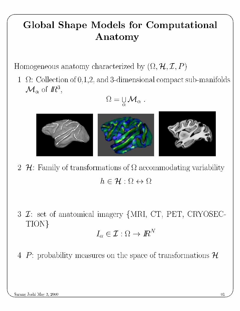
Homogeneous anatomy characterized by (;H; I; P ).

1. : Collection of 0,1,2, and 3-dimensional compact sub-manifolds

M� of IR3,

=[�M� :

2. H: Family of transformations of accommodating variability.

h 2 H : $

3. I : set of anatomical imagery fMRI, CT, PET, CRYOSEC-

TIONg .

I� 2 I : ! IR

N

4. P : probability measures on the space of transformations H.

'

&

$


Global Shape Models for Computational

Anatomy.

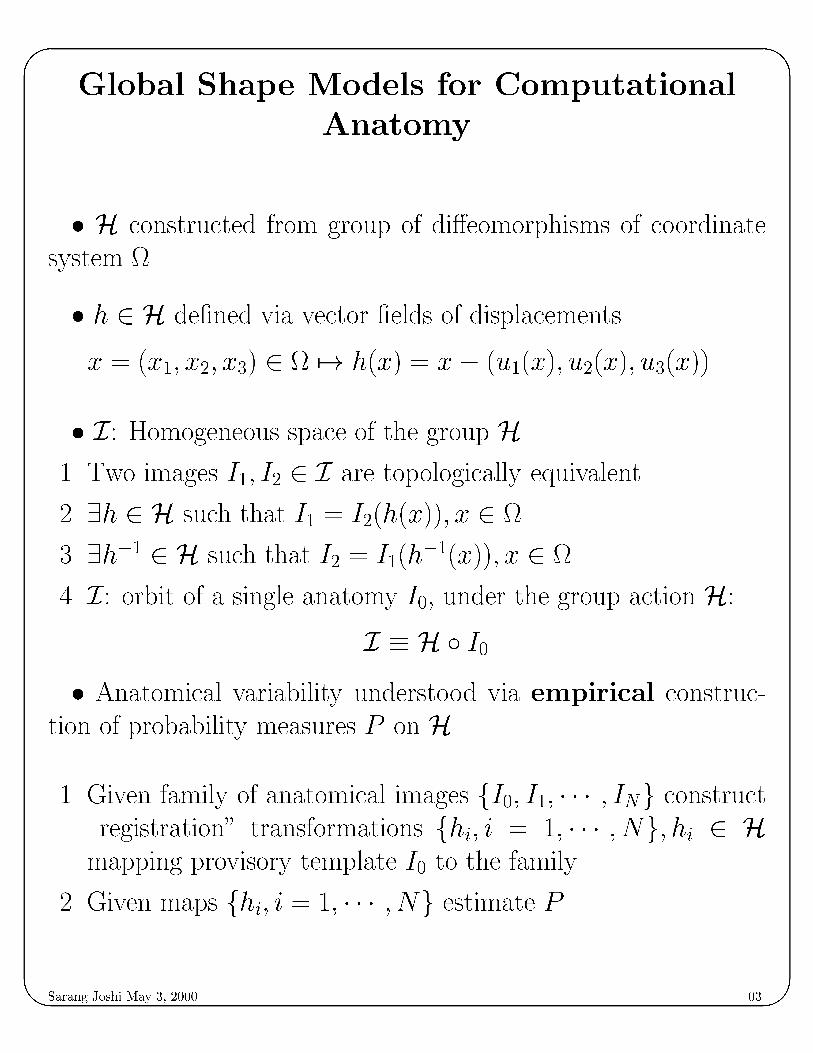
� H constructed from group of di�eomorphisms of coordinate

system .

� h 2 H de�ned via vector �elds of displacements.

x = (x1; x2; x3) 2 7! h(x) = x� (u1(x); u2(x); u3(x))

� I : Homogeneous space of the group H.

1. Two images I1; I2 2 I are topologically equivalent.

2. 9h 2 H such that I1 = I2(h(x)); x 2 .

3. 9h�1 2 H such that I2 = I1(h�1(x)); x 2 .

4. I : orbit of a single anatomy I0, under the group action H:

I � H � I0

� Anatomical variability understood via empirical construc-

tion of probability measures P on H.

1. Given family of anatomical images fI0; I1; � � � ; INg construct

\registration" transformations fhi; i = 1; � � � ; Ng; hi 2 H

mapping provisory template I0 to the family.

2. Given maps fhi; i = 1; � � � ; Ng estimate P .

'

&

$


Representation of Sub-Structures of the

Brain.

The surface M of neuro-anatomically signi�cant substructure

is assumed to be a smooth two-dimensional C2 sub-manifold of

� IR3.

� Build local quadratic charts.

xi

ni

b1xi

b2xi

xj

xpj

hj

Txi(M )

'

&

$


Shape of 2-D Sub-Manifolds of the Brain:

Hippocampus.

The provisory template hippocampal surfaceM0 is carried onto

the family of targets:

M0

h1�! �h

�11

M1;M0

h2�! �h

�12

M2; � � � ;M0

hN�! �h

�1N

MN:

h1

h2

hN

h1 o M0

h2 o M0

M0

Template

hN o M0

'

&

$



Hippocampus.

� The mean transformation and the template representing the

entire population:

�h =

1

N

NXi=1

hi ; Mtemp = �h �M0 :

The mean hippocampus of the population of thirty subjects.

'

&

$



Hippocampus.

� Mean hippocampus representing the control population:

�hcontrol =

1

Ncontrol

NcontrolXi=1

h

control

i; Mcontrol = �

hcontrol �M0 :

� Mean hippocampus representing the Schizophrenic popula-

tion:

�hschiz =

1

Nschiz

NschizXi=1

h

schiz

i; Mschiz = �

hschiz �M0 :

Control population Schizophrenic population

'

&

$


Gaussian Random Vector Fields on 2-D

Sub-Manifolds.

�HippocampiMi; i = 1; � � � ; N deformation of the meanMtemp:

Mi : fyjy = x + ui(x) ; x 2Mtempg

ui(x) = hi(x)� x; x 2Mtemp :

Vector �eld ui(x) shown in red.

� Construct Gaussian random vector �elds over sub-manifolds.

'

&

$



Sub-Manifolds.

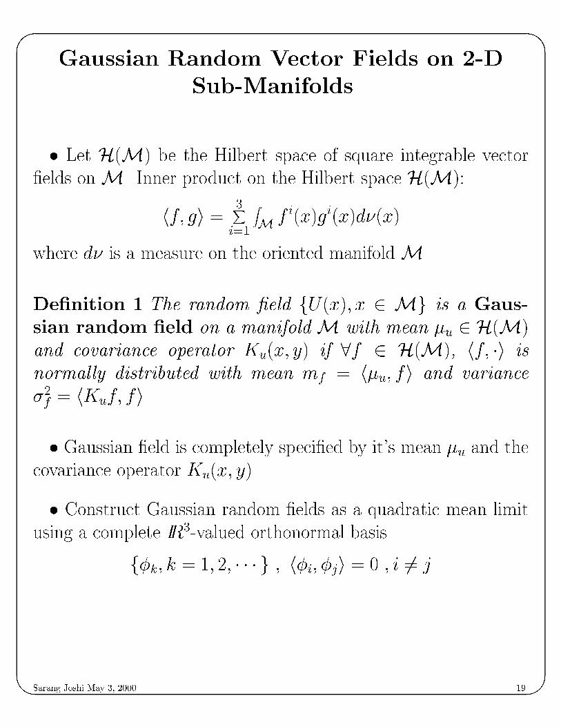
� Let H(M) be the Hilbert space of square integrable vector

�elds onM. Inner product on the Hilbert space H(M):

hf; gi =3Xi=1

ZMf

i(x)gi(x)d�(x)

where d� is a measure on the oriented manifoldM.

De�nition 1 The random �eld fU(x); x 2 Mg is a Gaus-

sian random �eld on a manifoldM with mean �u 2 H(M)

and covariance operator Ku(x; y) if 8f 2 H(M), hf; �i is

normally distributed with mean mf = h�u; fi and variance

�2f= hKuf; fi

� Gaussian �eld is completely speci�ed by it's mean �u and the

covariance operator Ku(x; y).

� Construct Gaussian random �elds as a quadratic mean limit

using a complete IR3-valued orthonormal basis

f�k; k = 1; 2; � � � g ; h�i; �ji = 0 ; i 6= j

'

&

$


Isotropic Stochastic Process on The Sphere:

Oboukhov expansion

� Let H(S) be the Hilbert space of square integrable functions on

the sphere S . Inner product on the Hilbert space H(S):

hf; gi =ZSf(�; �)g(�; �)sin(�)d�d�

where sin(�)d�d� is the measure on the sphere S .

� The Spherical Harmonics Y m

nare a complete orthonormal ba-

sis of H(S)

De�ne process fu(p); p 2 Sg

u(p) = limN!1

in q:m:

NXn=0

nXm=�n

ZnmYm

n(p) ;

where � Znm are zero mean independent Gaussian random vari-

ables with variance �n withP�n <1.

Theorem: The stochastic process fu(p); p 2 Sg constructed

above is an isotropic zero mean q.m. continuous Gaussian process

with covariance

K(x; y) =1Xn=0

�nPn(cos d(x; y))

'

&

$



Sub-Manifolds.

Theorem 1 Let fU(x); x 2Mg be a Gaussian random vector

�eld with mean mU 2 H and covariance KU of �nite trace.

There exists a sequence of �nite dimensional Gaussian random

vector �elds fUn(x)g such that

U(x)q.m.= lim

n!1Un(x)

where

Un(x) =nX

k=1Zk(!)�k(x) ;

fZk(!); k = 1; � � � g are independent Gaussian random vari-

ables with �xed means EfZkg = �k and covariances EfjZij2g�

EfZig2 = �

2i= �i;

Pi �i < 1 and (hk; �k) are the eigen func-

tions and the eigen values of the covariance operator KU :

�i�i(x) =ZMKU(x; y)�i(y)d�(y) ;

where d� is the measure on the manifoldM.

If d�, the surface measure on �Mtemp is atomic around the

points xk then f�ig satisfy the system of linear equations

�i�i(xk) =MXj=1

K̂U(xk; yj)�i(yj)�(yj) ; i = 1; � � � ; N ;

where �(yj) is the surface measure around point yj.

'

&

$


Eigen Shapes of the Hippocampus.

� Assume that deformation �elds fui(x); i = 1; � � � ; Ng are

realizations from a Gaussian �eld on the surface of the mean hip-

pocampusMtemp.

� Empirical estimate of the covariance operator given by

K̂U(x; y) =1

N � 1

NXi=1

ui(x)ui(y)T:

� Numerically compute the eigenfunctions and eigenvalues of

using Singular Value Decomposition:

1. Let f�(i); i = 1; � � � ; Ng be vectors of length 3M with

�(i)k = �i(xk)

2. � be a diagonal matrix of size 3M � 3M with

�3j;3j = �3j+1;3j+1 = �3j+2;3j+2 = �(yj);

3. K̂U be a 3M � 3M symmetric matrix with

K̂i;j = K̂U(xi; xj):

The system of linear equations in the above theorem becomes

�i�(i) = K̂��(i)

; i = 1; � � � ; N:

The basis vectors f�(i); i = 1; � � � ; Ng are generated by diago-

nalizing the matrix K̂�.

'

&

$


Eigen Shapes of the Hippocampus.

� Eigen shapes E i; i = 1; � � � ; N de�ned as:

E i = fx + (�i)�i(x) : x 2 �Mtempg :

� Eigen shapes completely characterize the variation of the sub-

manifold in the population.

'

&

$


Statistical Signi�cance of Shape Di�erence

Between Populations.

� Assume that fuschizj

; ucontrol

jg; j = 1; � � � ; 15 are realizations

from a Gaussian process with mean �uschiz and �ucontrol and common

covariance KU .

Statistical hypothesis test on shape di�erence:

H0 : �unorm = �uschiz

H1 : �unorm 6= �uschiz

�Expand the deformation �elds in the eigen functions �i:

u

schiz(j)N (x) =

NXi=1

Z

schiz(j)i �i(x)

u

control(j)N (x) =

NXi=1

Z

control(j)i �i(x)

� fZschiz

j; Z

control

j; j = 1; � � � ; 15g Gaussian random vectors

with means �Zschiz and �

Zcontrol and covariance �.

Hotelling's T 2 test:

T

2N=M

2( �̂Znorm � �̂

Zschiz)T �̂�1( �̂Znorm � �̂

Zschiz) :

N T2N

p-value : PN(H0)

3 9.8042 0.0471

4 14.3086 0.0300

5 14.4012 0.0612

6 19.6038 0.0401N: number of eigen functions.

'

&

$


Bayesian Classi�cation on Hippocampus

Shape Between Population.

� Bayesian log-likelihood ratio test: H0: normal hippocampus,

H1: schizophrenic hippocampus.

�N = �(Z � �̂Zschiz)

y�̂�1(Z � �̂Zschiz)

+ (Z � �̂Znorm)

y�̂�1(Z � �̂Znorm)

H0

<

>

H1

0

� Use Jack Knife for estimating probability of classi�cation:

-6

-4

-2

0

2

4

6

Control Schiz

Log

Like

lihoo

d R

atio

'

&

$


DISTRIBUTION FREE STATISTICAL

TESTING.

� Use Fisher's method of randomization to empirically estimate

the distribution of the test statistics with out the Gaussian as-

sumption.

� Under the null hypothesis H0 the expansion coe�cients

(ZN

i)schiz; Z

N

i)control) for i = 1; � � � ;M are independent random

samples from a single population.

� Each of the (2NN ) possible permutations of the data are equally

likely and can be used for estimating the distribution of the test

statistics under the hypothesis H0.

� For N = 15 , 1:551175e + 08 di�erent combinations.

� Use monte carlo simulations for estimating the probability

distribution by generating uniformly distributed random combi-

nations.

'

&

$


DISTRIBUTION FREE STATISTICAL

TESTING.

� Estimate probability distribution of the T 2 statistics under the

hypothesis H0 computed using 100000 monte carlo simulations.

0 1 2 3 4 5 6 7 80

0.02

0.04

0.06

0.08

0.1

0.12

0.14

0.16

0.18Number of Simulations = 100,000 P = 0.02320

� The signi�cance level or the p-value becomes:

P =Z1

T 2 F̂ (f)df :

� Using 4 eigen shapes the p-value is estimated at 0:0232

� Statistically signi�cant di�erence in the populations.

4000

3500

3000

2500

2000

1500

1000

Hip

poca

mp

us v

olu

me

(m

m3 )

Younger control CDR 0 CDR 0.5

L R L R L R

A

4000

3500

3000

2500

2000

1500

1000

Hip

poca

mp

us v

olu

me

(m

m3 )

Youngercontrol

ConsistentCDR 0

InconsistentCDR 0.5

ConsistentCDR 0.5

L R L R L R L R

B

John G. Csernansky, Lei Wang, Sarang Joshi, J. Philip Miller, Mohktar Gado, Daniel Kido, Daniel McKeel,John C. Morris, Michael I. Miller, “Hippocampal Deformities Distinguish Dementia of the Alzheimer Type fromHealthy Aging,” submitted to Science, 1999.

Inward, 3.3mm

Outward, 3.3mm

Inconsistent CDR 0.5 vs. Consistent CDR 0

R L R L

Consistent CDR 0.5 vs. Consistent CDR 0

Inconsistent CDR 0.5

Consistent CDR 0

p = .015

Consistent CDR 0.5

Consistent CDR 0

p = .0015

A

B

Log

-lik

elih

ood

ra

tio

Log

-lik

elih

ood

ra

tio

C

R L R L

Outward, p < 0.05

Inward, p < 0.05

p > 0.05


Inward, 3.3mm

Outward, 3.3mm

R L

R L

ConsistentCDR 0

Younger control

p < .001

Log

-lik

elih

ood

ra

tio

A

B

C

Consistent CDR 0 vs. Younger control

Outward, p < 0.05

Inward, p < 0.05

p > 0.05


Documents

Statistical - cs.unc.edu · tire p opulation: h = 1 N N X i =1 i; M temp 0: The me an hipp o c ampus of the p ... i; M 0: Mean hipp o campus represen ting the Sc ... Statistical Signi