STATISTICAL BACKGROUND FOR CBER PROPOSALS FOR ACCEPTABLE PROCESS CONTROL PLANS

John Scott, Ph.D.

Division of Biostatistics

FDA / CBER / OBE

October 19, 2012

Outline

Statistical Quality Control overview Sampling for quality control Single-stage sampling plans

Binomial plans Hypergeometric plans

Double-stage sampling plans Binomial plans Hypergeometric plans

Further possibilities

2

Statistical Quality Control Overview3

4

What is quality control?

Quality = “fitness for purpose” Many aspects to assessing quality, e.g.

Performance, reliability, durability, serviceability, aesthetics, features, perceived quality, conformance to standards

Much of the quality control literature centers on reduction of variability

We’re focused on assessing conformance Non-conformance is the end result of

uncontrolled variability

Methods of statistical quality control

Statistical process control methods Describe and explain variability in an

ongoing process Methods focus on graphical displays –

simple plots, Pareto charts, control charts

Experimental design methods Systematically assess sensitivity of

outputs to changes in input Acceptance sampling methods

Inspect and test final product for conformance

5

Some SPC graphs

Stem and leaf plot

Box plot Pareto chart The decimal point is 2 digit(s) to the left of the |

87 | 13

87 | 69

88 | 11233334

88 | 6788999

89 | 000011111223344444

89 | 556666677788888888889999

90 | 00001111112233344

90 | 5555666677778888

91 | 000000011122333333344

91 | 555556778

92 | 24444

92 | 6

Do

no

r

Op

era

tor

Filt

er

RBC Recovery Failures

Fre

qu

en

cy

05

10

15

20

0%

20

%4

0%

60

%8

0%

10

0%

Cu

mu

lativ

e P

erc

en

tag

e

6

Control charts

Control charts map samples of a product characteristic over time to identify when a process might be out of control

Features: A center line corresponding to the

average “in control” value Upper and lower control limits Out of control values or unusual runs

may be signals for investigation or action

7

Control chart example

RBC Recovery Control

Sample

% R

BC

Re

cove

ry

1 3 5 7 9 11 13 15 17 19 21 23 25

0.8

90

0.8

95

0.9

00

0.9

05

0.9

10

0.9

15

0.9

20

LCL

UCL

CL

8

Sampling for QC9

PopulationPopulation

Sample

Conformance to standards

The plateletpheresis and leukoreduction Guidances each recommend: Standards for QC testing of individual units A maximum acceptable proportion of non-

conforming units A minimum confidence level

Only process failures are counted as non-conforming Non-process failures (failures due to

uncontrollable parameters) are replaced in QC testing

10

Leukoreduction standards11

Plateletpheresis standards12

Maximum process failure rates 5% for:

Residual WBC content Content recovery / retention pH

25% for: Platelet yield

13

Minimum confidence levels

In each case, the Guidances recommend establishing a process failure rate below the maximum “with 95% confidence”

That means: if the true process failure rate for a given month is at the maximum allowable level, there’s: A 95% chance that QC testing will detect a problem,

or A 5% chance that the problem will go erroneously

undetected 95% confidence in a 95% success rate is

called “95%/95% acceptance” 95% confidence in a 75% success rate is

“95%/75% acceptance”

14

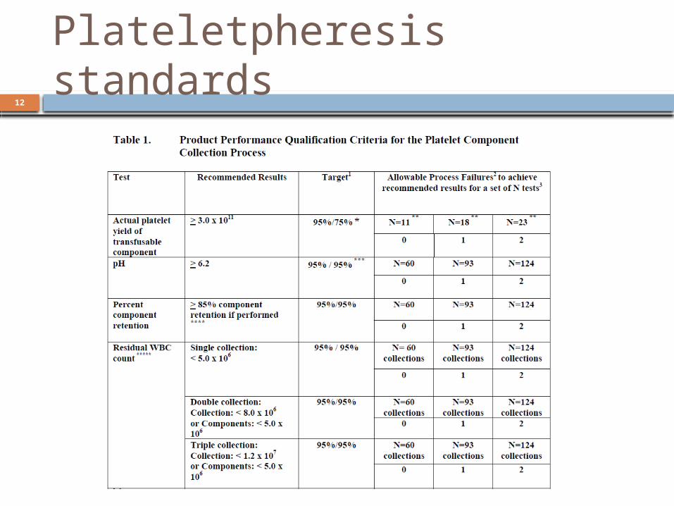
How to get to 95% confidence There’s an “easy” way to have 100%

confidence: test every unit. E.g.: Suppose you produce 200 units of RBC, LR

in a given month You test residual WBC content on every unit All but 8 units meet WBC < 5.0 x 106 The failure rate is 8/200 = 4% with 100%

confidence When testing every unit is impractical

(i.e. usually), you can use statistical sampling to get to 95% confidence

15

The logic of statistical sampling The population is what you

want to draw a conclusion about E.g. this month’s RBC units

Take a random sample, measure failure rate in the sample, use probability models to make inference about population rate Yields an estimate of population

rate Estimate has some uncertainty

because sample is incomplete

Population

Sam-ple

16

Acceptance sampling

Acceptance sampling consists of taking a sample from a lot and making a decision to accept or reject the lot based on the sample

Not the same as SPC for blood establishments A month’s worth of units is not a “lot” A month’s worth of units will not be

discarded on failed QC Common methods of acceptance

sampling do correspond to FDA recommendations

17

Acceptance sampling translations In order to use acceptance

sampling terminology, we need a couple translations

“Accept” = Pass QC testing for the month No further action required

“Reject” = Fail QC testing for the month Launch a failure investigation

18

Single-stage sampling plans

19

0.00 0.02 0.04 0.06 0.08 0.10

0.0

0.2

0.4

0.6

0.8

1.0

Single-stage sampling plans

In a given month, N units will be produced In a single-stage sampling plan:

A sample of n units is tested If more than c process failures, reject;

otherwise accept E.g. n = 60, c = 0 means:

We test a sample of 60 units If no process failures, accept If at least 1 process failure, reject, launch a

failure investigation n and c need to be chosen to provide

recommended confidence

20

Binomial single-stage sampling The Guidances recommend that n and c

be chosen such that the probability of accepting is at most 5% when the true failure rate is at the maximum allowed

We need a probability model to calculate the probability of accepting

For large N we usually use the binomial distribution Called “Type B sampling” in SPC literature

The binomial distribution assumes a random sample is taken with replacement from an infinite population

21

*The binomial distribution

Assume: The true failure rate is p The sample size is n The acceptance number is c

Then, under binomial sampling, the probability of accepting is given by:

For example, p = .05, n = 60, c = 0 gives

a probability of accepting of

22

0

!(1 )

!( )!

ck n k

k

np p

k n k

160

0

60!.05 (.95 .0)

!( )46

60 !k k

k k k

Operating characteristic curves For any sampling plan, we can ask:

what’s the probability of accepting at any given true failure rate? Recall that the Guidances recommend,

e.g., 5% probability of accepting at a true residual WBC failure rate of 5%

We also care about the probability of accepting at a “good” failure rate

An operating characteristic (OC) curve plots the probability of accepting against the true failure rate

23

OC curve examples24

0.00 0.02 0.04 0.06 0.08 0.10

0.0

0.2

0.4

0.6

0.8

1.0

OC Curves for type B sampling plans, n=93

Proportion of process failures

Pro

ba

bili

ty o

f acc

ep

tan

ce c=0, n=93c=1, n=93c=2, n=93

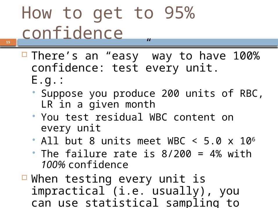
Practical binomial single-sampling Very few binomial single-stage sampling

plans are useful in practice Once you choose c, the smallest

allowable n is the best choice For 95%/95%:

1. c = 0, n = 59*2. c = 1, n = 933. c = 2, n = 124

*note that the Guidances mention c = 0, n = 60; establishments often prefer the round number, but c = 0, n = 59 is also acceptable

25

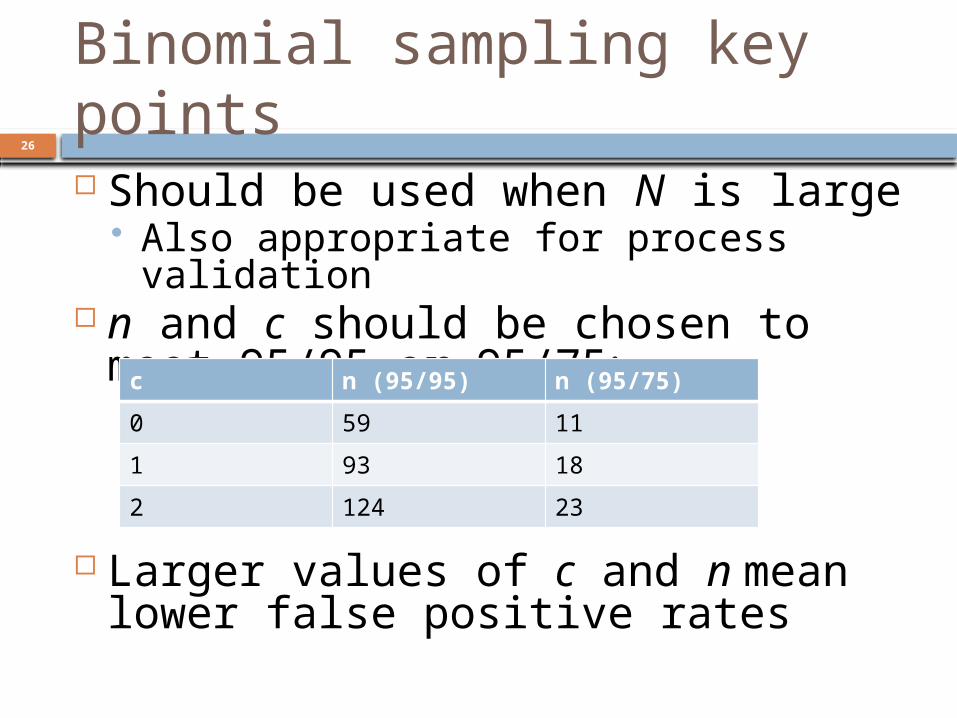
Binomial sampling key points Should be used when N is large

Also appropriate for process validation n and c should be chosen to meet

95/95 or 95/75:

Larger values of c and n mean lower false positive rates

26

c n (95/95) n (95/75)

0 59 11

1 93 18

2 124 23

Hypergeometric single-stage sampling The binomial distribution assumes

an infinite population You don’t produce an infinite number of

units, but this works well enough for large N

If the population is small, we can use the hypergeometric distribution instead Called “Type A sampling” in SPC

literature The hypergeometric distribution

assumes a random sample is taken without replacement from a finite population of size N

27

*The hypergeometric distribution Assume:

The population size is N The population number of successes is m

(m ≥ (1-p)N) The sample size is n The acceptance number is c

Under hypergeometric sampling, the probability of accepting is given by:

28

0

! ( )!!( )! ( )!( )!

!!( )!

c

k

m N mk m k n k N m n k

Nn N n

Hypergeometric OC curve examples

29

0.00 0.02 0.04 0.06 0.08 0.10

0.0

0.2

0.4

0.6

0.8

1.0

OC Curves for type A sampling plans (N=100)

Proportion of process failures

Pro

ba

bili

ty o

f acc

ep

tan

ce c=0, n=45c=1, n=65c=2, n=81

Binomial vs. hypergeometric plans Hypergeometric plans have

logistical difficulties: You need to know N (or put upper

bound on N) QC process may change from month to

month or component to component Binomial plans require larger

samples As N gets large, difference between

binomial and hypergeometric approaches narrows Almost no difference when N is at least

10 times bigger than n

30

Hypergeometric key points

Useful when N is small Sampling plan depends on knowing

N You may need to plan around an upper

bound on N Can’t be used for process validation For each N, you can choose n and c

to meet 95/95 or 95/75. E.g. for N = 100:

31

C n (95/95) n (95/75)

0 45 10

1 65 16

2 81 22

Single-stage sampling issues The sampling plan needs to be

prespecified Not acceptable to plan on c=1, n=93, then get

to 59 with no process failures and accept without further testing

You need to sample in such a way that you’ll have enough tests to meet QC acceptance rule With a c=1, n=93 sampling plan, if you have 1

process failure in 80 tests in a month, 95%/95% hasn’t been met

For small N, hypergeometric plans may involve testing almost 100% of units You may need to test consecutively from start

of month Potentially problematic if something changes

mid-month

32

Double-stage sampling plans

33

0.00 0.02 0.04 0.06 0.08 0.10

0.0

0.2

0.4

0.6

0.8

1.0

Double-stage sampling plans In a double-stage sampling plan:

A sample of n1 units is tested If c or fewer process failures are observed,

accept If c+2 or more process failures are

observed, reject If c+1 process failures are observed:

A second sample of n2 units is tested If no more process failures are observed,

accept If one or more process failures are observed,

reject c, n1 & n2 are chosen to meet

recommended criteria (e.g. 95%/95%, 95%/75%)

34

Binomial double-stage plans

For large N, we calculate probability of acceptance using the binomial distribution

Some acceptable double-stage sampling plans:

35

C 95/95 95/75

N1 n2 n1 n2

0 60 71 11 11

1 94 75 18 8

2 125 69 23 17

Double vs. single-stage sampling

36

0.00 0.02 0.04 0.06 0.08 0.10

0.0

0.2

0.4

0.6

0.8

1.0

OC Curves for single- vs. double-sampling

Proportion of process failures

Pro

ba

bili

ty o

f acc

ep

tan

ce c=0, n=59c=0, n1=60, n2=71c=1, n=93c=1, n1=94, n2=75c=2, n=124c=2, n1=125, n2=69

Flexibility in double-stage plans There are more choices with

double-stage plans All of these meet 95%/95%:

c n1 n2 Pr(accept) if p = 1%

Avg. total n if p = 1%

Max n

0 59 90 69% 89 149

0 60 71 71% 84 131

0 61 61 72% 82 122

0 62 55 73% 81 117

37

Hypergeometric double-sampling As with single-stage sampling,

binomial double-stage sampling is pretty efficient if N is large

For small N, hypergeometric double-stage sampling may allow smaller samples

You need to know N (or be able to put an upper bound on it)

The calculations are a little complicated; Appendix A of the leukoreduction guidance provides a table

38

Hypergeometric double-stage sampling examples

39

Double-stage sampling issues As with single-stage sampling:

Pre-specification required Need to ensure enough units are tested

Note that many hypergeometric plans have a second stage of 100% (“ALL”) or almost 100% You can’t get to 100% if you skipped any For N=50, c=0, n1=31, n2=18, you may be

done with testing two weeks into the month Will you catch issues late in the month? Supplemental testing may be advisable

40

Double-stage sampling key points Adopting a double-stage sampling

plan: Gives you a chance to “rescue” a

process in the event of a failed test Reduces risk of false positives

Binomial plans are appropriate for large N

Hypergeometric plans yield smaller sample sizes for small N Can’t be used for process validation

Plans should be pre-specified

41

Other Possibilities42

Multiple-stage sampling

Double-stage sampling can be generalized: The second stage can be designed

to allow for 1 or more process failures

Third, fourth, or … stages can be added

None of these techniques are likely to lead to practical sample sizes in the blood establishment setting

43

Chain sampling

In chain sampling, a sample of size n would be taken each month

If 0 process failures, accept If 2 process failures, reject If 1 process failure:

Accept if there have been 0 process failures in the past i months

Otherwise reject Hasn’t been proposed, to my

knowledge

44

Scan statistics

Scan statistics can be used to continuously monitor an ongoing process to look for event clusters

How it works: N tests over a year Look at every possible sequence of m

consecutive tests (a “window”) If there are more than k failures in a

window, the process is out of control N, m and k chosen to achieve probability of

declaring: In control at a “good” failure rate, p1 (e.g. 1%) Out of control at a “bad” failure rate, p2 (e.g.

5%)

45

Scan statistic pros and cons

A natural way to look at blood product QC Months are arbitrary (although c.f. CFR)

Avoids issues related to non-random sampling

Mathematically & logistically complex No free lunch!

Added flexibility of the scan statistic comes at a price

If you want 95%/95% for any scan window, large N (e.g. N > 1000) required, or false positives high

Compare to 60/month binomial N = 720

46

Thanks!47