Statistical Analysis of Urban Design Variables and - State of Oregon

��

��

6677$$77,,6677,,&&$$//��$$11$$//<<66,,66��22))��8855%%$$11��''((66,,**11��99$$55,,$$%%//((66��

$$11''��77++((,,55��8866((��,,11��7755$$99((//��''((00$$11''��0022''((//66��

��

1RYHPEHU��3UHSDUHG�IRU��3HUIRUPDQFH�0HDVXUHV�6XEFRPPLWWHH�RI�WKH�2UHJRQ�0RGHOLQJ�6WHHULQJ�&RPPLWWHH��3UHSDUHG�E\�� /DQH�&RXQFLO�RI�*RYHUQPHQWV�3RUWODQG�0HWUR�2UHJRQ�'HSDUWPHQW�RI�7UDQVSRUWDWLRQ�

Principal Researchers/Authors: Bud Reiff, Lane Council of Governments

Chair, Performance Measures Subcommittee of the Oregon Modeling Steering Committee

Kyung-Hwa Kim, Portland Metro Reviewers: William Upton, Oregon Department of Transportation Brian Gregor, Oregon Department of Transportation Richard Walker, Portland Metro Staff Support: Michal Wert, MW Consulting

Copyright @2003 by the Oregon Department of Transportation. Permission is given to quote and reproduce parts of this document if credit is given to the source. This project was funded in part by the Federal Highway Administration, U.S. Department of Transportation. Copies of this document are available on the ODOT website at www.odot.state.or.us/tddtpau/modeling.html or from: William J. Upton Oregon Department of Transportation Transportation Planning Analysis Unit 555 13th Street Salem, OR 97301 Telephone: 503-986-4106 Email: [email protected]

______________________________________________________________________________________________ Statistical Analysis of Urban Design Variables and Their Use in Travel Demand Models i

TABLE OF CONTENTS

TABLE OF CONTENTS .......................................................................................... i EXECUTIVE SUMMARY....................................................................................... iii INTRODUCTION....................................................................................................1 RECENT STUDIES ................................................................................................2 SELECTED VARIABLES........................................................................................2 DATA-SET PREPARATION ...................................................................................4

Composite Urban Design Measures Test I ........................................................ 5 Composite Urban Design Measures Test II ........................................................6 Composite Urban Design Measures Test III .......................................................6 Composite Urban Design Measures Test IV.......................................................7

STATISTICAL ANALYSIS IN THE AUTO-OWNERSHIP MODEL..........................9 STATISTICAL ANALYSIS IN THE MODE CHOICE MODEL ...............................11

Simple Regression Model 1 ..............................................................................12 Simple Regression Model 2 ..............................................................................12 Home-Based-Other Mode Choice Model 1 .......................................................13 Home-Based-Other Mode Choice Model 2 .......................................................14 Home-Based-Other Mode Choice Model 3 .......................................................14 Home-Based-Other Mode Choice Model 4 .......................................................15

MIXED LAND USE SENSITIVITY TEST ..............................................................15 REPRESENTATIVE SAMPLE LOCATIONS ........................................................17 CONCLUSIONS ...................................................................................................18 APPENDIX 1: REFERENCES APPENDIX 2: URBAN DESIGN VARIABLES CONSIDERED APPENDIX 3: URBAN DESIGN VARIABLES EVALUATED MAP FOLLOWING APPENDIX 3: REPRESENTATIVE SAMPLE LOCATIONS List of Tables Table 1. Example of Normalization Procedure---------------------------------------------5 Table 2. Mixed I Calculation Result Summary --------------------------------------------5 Table 3. Mixed II Calculation Result Summary -------------------------------------------6 Table 4. Mixed III Calculation Result Summary------------------------------------------7 Table 5. Mixed IV Calculation Result Summary ------------------------------------------8 Table 6. Auto Ownership Model with Urban Accessibility Variable Test ---------- 10 Table 7. Correlation Matrix -------------------------------------------------------------------- 11 Table 8. Home-Based-Other Mode Choice Model-------------------------------------- 13 Table 9. Home-Based-Other Mode Choice Model-------------------------------------- 14 Table 10. Non-Auto Mode and Land use Data Summary by Four Areas--------- 15

______________________________________________________________________________________________ Statistical Analysis of Urban Design Variables and Their Use in Travel Demand Models ii

______________________________________________________________________________________________ Statistical Analysis of Urban Design Variables and Their Use in Travel Demand Models iii

STATISTICAL ANALYSIS OF URBAN DESIGN VARIABLES AND THEIR USE IN TRAVEL DEMAND MODELS

EXECUTIVE SUMMARY

Many travel demand models do not account for land use mixing and urban design effects. The purpose of this study is to further the understanding of how aspects of urban design influence transportation choices. This research identifies where it is important for models to account for urban design issues and where there would be minimal or no effect. It is intended to show how much land use change is necessary to significantly affect travel behavior. An extensive review was conducted of numerous recent studies that investigated the relationships between travel and the mixed-use and pedestrian-oriented design elements of urban areas. Simple statistical correlations have suggested that these elements can encourage shorter trips and trips by non-auto modes but the more rigorous studies have been largely inconclusive. The research identified eight specific urban design variables for further investigation. These generally fell into one of two categories: those related to accessibility (quantitative) and those related to other characteristics of the urban environment (qualitative). The accessibility variables affect the accessibility of destinations by various modes of travel or increase accessibility to other activities. These included: Census block density, dissimilarity index, entropy index, less auto-dependent urban form, residential parking permit districts and proximity to retail business establishments. The environmental variables included skinny streets and building coverage ratio.1 Each variable was studied to determine feasibility for data development and testing. The environmental variables proved to be too difficult to quantify using currently available Geographic Information System (GIS) data and software but should be considered in the future as necessary data and software become available. Several of the accessibility variables were also technically complex and difficult to forecast. Model estimation data was prepared for the Census block, business establishment and residential parking permit variables. These variables were tested using 1994/1995 Oregon Household Survey Data, along with three other accessibility-related variables currently used in the Portland Metro models. These include local street intersections, household density and employment density. The accessibility variables proved to be closely correlated with one another. It was surmised that they are also closely related to, and therefore would be co-linear with, the other accessibility and environmental variables. For example, increasing the variety of uses in close proximity produces a more attractive pedestrian environment.

1 Some variables are not clearly quantitative or qualitative and judgment was required to categorize the variable.

______________________________________________________________________________________________ Statistical Analysis of Urban Design Variables and Their Use in Travel Demand Models iv

Each of the correlated variables showed significance when tested alone. When tested together, some variables failed statistical tests for significance. Based on this evaluation, the focus of the remainder of the study was directed at developing a measure that captured multiple aspects of an accessible mixed-use development pattern. This measure includes: � The density of local street intersections - where intersections are more prevalent, walk and

bike distances tend to be shorter. � The density of households - with higher densities the average distance between households is

shorter, making walking and bicycling easier and more cost-effective to serve with transit. � The density of retail businesses - higher densities mean shorter travel distances, making it

easier for people to shop without using a car and to chain shopping trips together by walking, biking and/or public transit.

A test data set was prepared by compiling the number of local intersections, households and retail business establishments within a half-mile of each household included in the Household Survey Data. Three methods to combine these variables into a composite urban design measure were tested: fuzzy logic, factor analysis and harmonic mean. The results for the three methods were not significantly different and the latter method proved to be easiest to implement. An examination of the results for various neighborhood prototypes indicated that the relative significance of each component was preserved in the composite urban design measure. The composite urban design measure was tested to determine its effect on both auto ownership and mode choice. In the case of auto ownership, the composite measure did not improve overall explanatory power of the existing model of auto ownership choices which depends on household size, number of workers and income. In the case of mode choice, the composite urban design measure was found to be important in predicting mode choices. Sensitivity tests were conducted to see how changes in the composite urban design measure would affect the predicted use of non-automobile travel modes. To do this, all areas of the Portland region were stratified into four neighborhood types representing different levels of the composite urban design measure. Type 1 is characterized by discontinuous streets, low-density housing and no retail goods and services, such as the East Portland/Johnson Creek area. Type 2 has somewhat better street connectivity, higher residential density and/or access to retail businesses, such as parts of Lake Oswego. Type 3 has even more of the characteristics of a mixed-use urban neighborhood, such as Garden Home. Type 4 is characterized by a regular street grid, medium- to high-density residential neighborhoods and integral retail businesses, such as the NW 21st/23rd Avenue neighborhood. A summary of neighborhood-type characteristics is included in the following table.

______________________________________________________________________________________________ Statistical Analysis of Urban Design Variables and Their Use in Travel Demand Models v

Characteristic Type 1 Type 2 Type 3 Type 4

Portion of Portland Metropolitan Area 40% 30% 20% 10%

Non-Automobile Mode Share 4.69% 8.96% 12.66% 32.33%

Average Number of Households within ½ mile of TAZ*

976 1779 2869 4567

Average Number of Retail Businesses within ½ mile of TAZ*

3 19 35 121

Average Number of Local Intersections within ½ mile of TAZ*

65 103 168 232

Value of Urban Design Variable 19 128 399 1496

Average Number of Retail Employees within ½ mile of TAZ*

125 570 762 2447

Employees/Retail Business 36 30 22 20 *The Metro area was divided into about 1300 Transportation Analysis Zones for analytical purposes.

Average Value by Neighborhood Type For the initial testing, the value of the composite urban design measure was increased by 10 percent, 20 percent and 30 percent in each of the area prototypes. This corresponded to changes in one or more of the component variables ranging from modest to fairly substantial. Since the values of the composite urban design measure for nearly three-quarters of the Portland area were less than 10 percent of the average values for neighborhoods of Type 4, these marginal increases proved to be ineffective at reducing predicted automobile use. Even the 30 percent across-the-board increase in the composite urban design measure resulted in only half of a percent reduction in predicted auto use.2 An additional sensitivity test was performed to see what would happen if all the neighborhoods classified as Type 3 were changed so that their composite urban design values matched the average for neighborhoods classified as Type 4. To do this the values of the composite urban design measures for these neighborhoods was increased an average of 275 percent. Major land use and street system changes would need to occur to achieve this increase. Such a change is estimated to result in a 44 percent increase in predicted non-auto mode trips and a 6.5 percent reduction in auto use in the area affected. The regional effects would be smaller. However, the benefits may be underestimated for reasons noted above. 2 This reduction may be somewhat underestimated, since the kind of urban design changes necessary to achieve the 30 percent increase would also be likely to affect trip distances and transit accessibility. These were not varied in the sensitivity testing.

______________________________________________________________________________________________ Statistical Analysis of Urban Design Variables and Their Use in Travel Demand Models vi

Conclusions This study tested the relationship between mixed land use patterns and travel behavior. Conclusions of this research include: � A simple mixed-use variable that incorporates measures of residential density, employment

density and local street intersection density is useful for predicting travel mode choice. � There is a strong statistical association between this mixed-use variable and mode choice. � A statistical model which incorporates this variable explains mode choice behavior better

than a model which includes the elements of this measure separately, confirming the concept that land use mixing is useful and probably has some real effect on mode choice behavior.

� This mixed-use variable did not have a significant effect on auto ownership decisions. � Across the board increases in land use mixing of up to 30 percent has minimal effects on

regional auto travel (less than one percent) because most of the region has low mixing values and the effects of mixing are small until values are relatively large.

In summary, while land use mixing does influence mode choice behavior and this influence can be captured in urban travel models, the amount of influence is relatively small. Very large increases in residential, employment and street densities are necessary to achieve even modest decreases in automobile use.

______________________________________________________________________________________________ Statistical Analysis of Urban Design Variables and Their Use in Travel Demand Models 1

STATISTICAL ANALYSIS OF URBAN DESIGN VARIABLES AND THEIR USE IN TRAVEL DEMAND MODELS

INTRODUCTION Many planners and policy makers are concerned with the effects of urban design and mixed-use development on transportation choices. Several statistical surveys suggest that mixed-use development patterns are influential in encouraging shorter trip lengths and the use of non-single occupancy vehicle (SOV) travel modes. However, the conclusions derived from researchers are mixed. Numerous urban design characteristics potentially affect travel behavior. A number of these affect the accessibility of destinations by various modes of travel. For example, if more stores are located within walking distance of a residential neighborhood, then it will be easier for residents to walk to a store to shop. Similarly, if buses run more frequently thus reducing wait time to catch a bus, then people can go more places in the time they have available. This increases accessibility to other activities. A number of other urban design characteristics do not affect accessibility, but may make walking, bicycling or using public transportation more desirable. These could include skinny streets, street trees, building orientation and the amount of parking lots. Portland Metro’s travel demand model uses several urban design variables including mixed land use, retail employment within one mile, total employment within 30 minutes by transit, and number of intersections of local streets. These urban design variables are accessibility-related measures and are correlated with each other. This and the lack of detailed data make it difficult to understand the impacts of individual urban design elements on travel. The purpose of this research is to better understand the effects of urban design variables so that they can be incorporated into urban travel demand models. This will allow the transportation impacts of urban design policies to be estimated. This research focuses on the accessibility characteristics of urban design variables and their impact on travel behavior. Refining and testing these types of variables leads to a better understanding of urban design variables in transportation models. The study did not address other urban design characteristics. Data to objectively describe these are relatively difficult to obtain and to forecast and are an area for future research. This report is organized into the following elements: � Introduction � Research into the most recent studies of urban design variables � Selection of the final urban design variables to test � Preparing the data to calculate the final urban design variables � Performing statistical analyses and estimating the auto-ownership model with the final urban

design variables � Analyzing urban design variables in the mode choice model


� Carrying out a mixed land-use sensitivity test � Developing a representative sample area � Conclusions This research project is sponsored by the Oregon Modeling Steering Committee (OMSC). The OMSC Performance Measurements Subcommittee provided research and project oversight. Lane Council of Governments (LCOG), Portland Metro (Metro), and the Oregon Department of Transportation (ODOT) staff were responsible for data preparation, model estimation, and analysis of the model results and data. RECENT STUDIES Metro and LCOG staff summarized current urban design research conducted in the United States and other countries. This included papers from the Transportation Research Board (TRB), the Federal Transportation Model Improvement Program (TMIP), and research by the consulting firm Parsons Brinckerhoff Quade and Douglas. Studies reviewed, definitions, sources, required data to calculate the value, and an assessment regarding the degree of difficulty to prepare the variables are included in the references in Appendix 1. The categories of urban design variables considered include:

Accessibility Diversity Balance Neighborhood Design Connectivity Pedestrian-oriented Crime Transit-oriented Density

SELECTED VARIABLES The many variables were categorized into one of two types: quantitative and qualitative. Quantitative variables are more objective and can be easily measured. They deal with land use variety, circulation efficiency and proximity. Qualitative variables are more subjective and deal with the human interaction aspects of urban design that are more difficult to measure, such as building orientation, pedestrian safety and streetscape. It is recognized that the distinction between quantitative and qualitative measures is not always clear and some judgment was required to define these measures. Appendix 2 lists these variables. After studying the most current research, eight variables were chosen for further analysis based primarily upon their potential for producing significant results. These included skinny streets, Census blocks, dissimilarity index, building coverage, residential parking permit, less auto-dependent urban form (LADUF), entropy index and business establishments. Each variable was analyzed for the feasibility and implementation of use. Following is a summary of the analyses of each urban design variable. They are defined and discussed in more detail in Appendix 3.


Skinny streets - This typically refers to local streets having a paved width less than 30 feet and a corner turning radius of less than 10 feet. The purpose of skinny streets is to slow traffic and make a friendlier environment for pedestrians. Collecting and forecasting this data is difficult. Census blocks - The number of Census blocks is correlated to the number of local intersections and other measures of population density. This variable is difficult to forecast for large, currently undeveloped tracts. Dissimilarity index - The dissimilarity index is a measure of land use mixing. It is a measure of the degree to which differing land uses come into contact with one another. It is calculated by dividing areas into grids, characterizing each grid cell by the predominant land use, and then evaluating the similarity between each grid cell and its neighbors. The results of this measure depend on the choice of grid cell size and the number of land use categories. For example, if the grid cells are small and the number of land use categories is few, the result is a fairly low level of dissimilarity. The complexity of this measure makes it difficult to compute and forecast. Mean entropy - Entropy is an indicator of land use balance and is like the dissimilarity index. It measures the uniformity in dispersion of various development types. The analysis of this variable is fairly complex and presents some technical challenges to implement. Entropy is not an easy variable to explain to non-technical public and elected officials. Building coverage index - Building coverage is the proportional land area occupied by buildings. It is associated with a number of urban design attributes, including building orientation, parking supply and orientation, setback, streetscape and density. This variable will likely require aerial photography interpretation software in order to be efficiently produced for an entire urban area. It is not clear how parking structures should be handled. Less auto-dependent urban form (LAUDF) -This is a composite urban design variable. The value combines measures for density, land use mix and circulation using 150 meter grid cells as the geographic unit of analysis. Although current data is readily available to compute the values, the analysis required to calculate a measure that maximizes its explanatory power is complex and difficult. It is also difficult to forecast this measure. Residential parking permit areas - The residential parking permit areas are neighborhoods in which long-term weekday on-street parking is available only to area residents with parking permits. These areas tend to be centrally located near major attractors such as retail, service and employment centers. This variable is similar to other accessibility variables because areas where residential parking permits are required tend to be older neighborhoods where there is good street connectivity, bus service, sidewalks and proximity to downtown areas. This variable was found not to be a strong predictor of auto ownership. Business establishments -Retail and service activities are typically represented in models by employment. However, they can also be represented by retail and service business establishments. While employment is an appropriate indicator of the number of primary trips


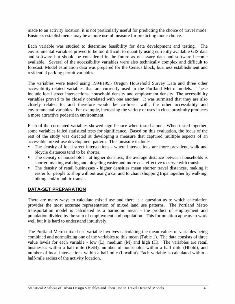
made to an activity location, it is not particularly useful for predicting the choice of travel mode. Business establishments may be a more useful measure for predicting mode choice. Each variable was studied to determine feasibility for data development and testing. The environmental variables proved to be too difficult to quantify using currently available GIS data and software but should be considered in the future as necessary data and software become available. Several of the accessibility variables were also technically complex and difficult to forecast. Model estimation data was prepared for the Census block, business establishment and residential parking permit variables. The variables were tested using 1994/1995 Oregon Household Survey Data and three other accessibility-related variables that are currently used in the Portland Metro models. These include local street intersections, household density and employment density. The accessibility variables proved to be closely correlated with one another. It was surmised that they are also closely related to, and therefore would be co-linear with, the other accessibility and environmental variables. For example, increasing the variety of uses in close proximity produces a more attractive pedestrian environment. Each of the correlated variables showed significance when tested alone. When tested together, some variables failed statistical tests for significance. Based on this evaluation, the focus of the rest of the study was directed at developing a measure that captured multiple aspects of an accessible mixed-use development pattern. This measure includes: � The density of local street intersections - where intersections are more prevalent, walk and

bicycle distances tend to be shorter. � The density of households - at higher densities, the average distance between households is

shorter, making walking and bicycling easier and more cost effective to serve with transit. � The density of retail businesses - higher densities mean shorter travel distances, making it

easier for people to shop without using a car and to chain shopping trips together by walking, biking and/or public transit.

DATA-SET PREPARATION There are many ways to calculate mixed use and there is a question as to which calculation provides the most accurate representation of mixed land use patterns. The Portland Metro transportation model is calculated as a harmonic mean - the product of employment and population divided by the sum of employment and population. This formulation appears to work well but it is hard to understand intuitively. The Portland Metro mixed-use variable involves calculating the mean values of variables being combined and normalizing one of the variables to this mean (Table 1). The data consists of three value levels for each variable - low (L), medium (M) and high (H). The variables are retail businesses within a half mile (RetB), number of households within a half mile (Hhold), and number of local intersections within a half mile (Localint). Each variable is calculated within a half-mile radius of the activity location.


RetB Hhold Localint L 6 1012 68 M 21 1814 112 H 71 3825 215

Mean 32 2217 132

Normalize factor to RetB 69.3 (2217/32) 4.13 (132/32) L-low; M-medium; H-high; RetB-retail businesses within a half mile; Hhold-households within a half mile; Localint-local intersections within a half mile

Table 1. Example of Normalization Procedure

Four tests of composite urban design measures were conducted using a harmonic mean to produce the composite measures. Composite Urban Design Measures Test I � Calculate a new-scaled household variable that is normalized to the smaller mean, which is a

retail business. � Calculate harmonic mean. This variable is called the mixed-use variable.

Mixed I = ( RetB * (hhold/69.3)) / (RetB + (hhold/69.3)) The mixed I measure is an abstract one and is not easy to understand. Table 2 expresses the calculation in terms of three sample gradations. The RetB and Normhh variable values were chosen for illustrative purposes.

Combine Rank RetB Normhh Mixretbhh L-L 9 6 15 4 L-M 8 6 26 5 L-H 7 6 55 5.5 M-L 6 21 15 8.6 M-M 5 21 26 11.6 M-H 3 21 55 15.2 H-L 4 71 15 12.1 H-M 2 71 26 19.1 H-H 1 71 55 31.0

L-low; M-medium; H-high; RetB-retail businesses within a half mile; Normhh-normalized value for households within a half mile; Mixretbhh-mixed value with retail business and households

Table 2. Mixed I Calculation Result Summary


The first column indicates the combined relationship between number of retail businesses (High, Medium, Low) and number of households (High, Medium, Low). The rank column represents the order of the mixed value result. A lower rank suggests a higher mixed land use value. For example, a transportation analysis zone (TAZ) with a medium number of retail businesses and a high number of households has a higher mixed value compared to a TAZ with a high number of retail businesses and a low number of households. Composite Urban Design Measures Test II � Calculate a retail business variable, normalized to highest mean, which is number of

households. � Calculate Mixed II.

Mixed II = ( (RetB *69.3)* (hhold) ) / ( (RetB*69.3) + (hhold)) Test II was done to determine the effect of normalizing to household. The same illustrative variable values as in Table 2 are used in the calculation. Table 3 shows that the two tests result in the same ranking scheme.

Combine Rank Nor_retb Hhold Mixretbhh L-L 9 416 1012 295 L-M 8 416 1814 338 L-H 7 416 3825 375 M-L 6 1455 1012 597 M-M 5 1455 1814 807 M-H 3 1455 3825 1054 H-L 4 4919 1012 839 H-M 2 4919 1814 1325 H-H 1 4919 3825 2152

L-low; M-medium; H-high; Nor_retb-normalized value for retail businesses within a half mile; Hhold-households within a half mile; Mixretbhh-mixed value with retail business and households

Table 3. Mixed II Calculation Result Summary

Composite Urban Design Measures Test III � Test III was executed to quantify the impact of omitting the normalization process. � Calculate Composite III without normalization.

Mixed III = (RetB * hhold) / (RetB + hhold) The larger number in this mixed-use formula usually influences this calculation. In this case, number of households has more influence than the number of retail businesses (Table 4). The


most effective mixed-use design is one that is “big” and the household and employment are in balance.

Combine Rank Retb Hhold Mixretbhh L-L 9 6 1012 5.96 L-M 8 6 1814 5.98 L-H 7 6 3825 5.99 M-L 6 21 1012 20.57 M-M 5 21 1814 20.76 M-H 4 21 3825 20.89 H-L 3 71 1012 66.35 H-M 2 71 1814 68.33 H-H 1 71 3825 69.71

L-low; M-medium; H-high; RetB-retail businesses within a half mile; Hhold-households within a half mile; Mixretbhh-mixed value with retail business and households

Table 4. Mixed III Calculation Result Summary

These three tests showed how the mixed harmonic mean value is calculated. Test I or Test II is preferred since variables are normalized before calculating the mixed values. This normalization effect accounts for the problem when the average value of one variable is much larger and influences the value of the mixed calculation. Composite Urban Design Measures Test IV Harmonic means can also be tested with three variables - number of retail businesses (RetB), number of households (hhold) and number of local intersections (locint). � Calculate new-scaled household and local intersection variables that are normalized to the

smaller mean, which is a retail business. � Calculate harmonic mean with three variables. This variable is called the mixed-use

variable. The following formula shows how a three dimensional harmonic mean value is calculated.

Mixed IV (ret,hh,locint) =

( RetB * (hhold/69.3) * (locint/4.13) ) / (RetB + (hhold/69.3)+ (locint/4.13)) Table 5 suggests that the ranking is due to the well-balanced combination of the three variables. The highest mixed value in this table is the consequence of a well-balanced value of H-H-H for retail, households and intersections. Intuitively, the result is reasonable. If any low category is among the combination, the mix value has a lower rank than another combination near its


category. For example, the M-M-L combination has a rank of 17 while M-M-M has a rank of 13 and M-L-H has a rank of 14. Furthermore, the combination with the first rank has the best mixed-use while the combination with the last rank of 27 has the worst mixed use.

Combine Rank RetB Normhh Norlint Mixretbhhlint L-L-L 27 6 15 16.48 38.95

L-L-M 26 6 15 27.15 49.83 L-L-H 24 6 15 52.12 62.81 L-M-L 25 6 26 16.48 53.21 L-M-M 22 6 26 27.15 71.89 L-M-H 20 6 26 52.12 97.13 L-H-L 23 6 55 16.48 70.29 L-H-M 19 6 55 27.15 101.79 L-H-H 16 6 55 52.12 152.35 M-L-L 21 21 15 16.48 97.07 M-L-M 18 21 15 27.15 132.71 M-L-H 14 21 15 52.12 182.25 M-M-L 17 21 26 16.48 142.37 M-M-M 13 21 26 27.15 200.84 M-M-H 9 21 26 52.12 288.60 M-H-L 12 21 55 16.48 206.19 M-H-M 8 21 55 27.15 304.56 M-H-H 4 21 55 52.12 470.89 H-L-L 15 71 15 16.48 167.46 H-L-M 11 71 15 27.15 249.73 H-L-H 7 71 15 52.12 392.48 H-M-L 10 71 26 16.48 269.61 H-M-M 6 71 26 27.15 405.96 H-M-H 3 71 26 52.12 648.98 H-H-L 5 71 55 16.485 452.85 H-H-M 2 71 55 27.152 694.00 H-H-H 1 71 55 52.121 1145.69

L-low; M-medium; H-high; RetB-retail businesses within a half mile; Normhh-normalized value for households within a half mile; Norlint-normalized value for number of local intersections; Mixretbhhlint-mixed value with retail business, households and local intersections

Table 5. Mixed IV Calculation Result Summary


STATISTICAL ANALYSIS IN THE AUTO-OWNERSHIP MODEL Numerous statistical analyses were tested comparing the different urban design variables in the auto ownership model. The auto ownership model used the 1994/1995 Household Survey Data in the analysis. Multiple variables were used in the estimation, including several combined design variables such as the multi-modal-accessibility-logsum value, and a mixed land use variable (retb, hhold, locint). In addition, Brian Gregor from the Oregon Department of Transportation created a model that used “fuzzy logic”3 to combine the accessibility variables. This fuzzy logic model combined number of households and workplace proximity to produce a fuzzy logic mixed-use variable. A factor value combining retail, household and local intersection was also developed and used in estimating the auto-ownership model. Following is a list of the variables with definitions: � HHhm: number of household by half mile � Rethm: number of retail employment by half mile � RetBhm: number of retail business by half mile � ServBhm: number of service business by half mile � RetB1m: number of retail business by one mile � MutAcc: logsum of multi accessibility value from mode choice model (value includes eleven

mode constants, impedance, cost, accessibility) � Totemphm: total employment by half mile � TotBhm: total business by half mile � Totemp30T: total employment within 30 minutes by transit � Locinthm: local intersection by half mile � Ret.ratio hm/1m: retail employment by half mile/ retail employment by 1 mile � Ret.ratio hm/Max: retail employ by half mile/maximum retail employ by half mile � Fuzzmixhm: fuzzy mixed value of household, retail, and intersection by half mile � Mixrethhhm: mixed, retail and household by half mile � MixretBhhhm: mixed, retail business and household by half mile � Mixtotemphhhm: mixed, total employment and household by half mile � FactretBhhlinthm: factor, retail business, household, local intersection by half mile � MixretBhhlinthm: mixed, retail business, household, local intersection by half mile � Dwelling: single dwelling vs. multi dwelling � Hhsize: household size � Income: household income � Work4: number of workers (0,1,2,3) When tested individually, the accessibility-related variables showed strong statistical significance and explanatory power. The T-statistics and R-square of each accessibility variable in the auto-ownership regression model was similar (Table 6). Thus any one of these variables will not change the model conclusions. Each of these variables explains the same statistical property. Moreover the variables are highly correlated to each other.

3 Documented in a spreadsheet "FuzzyMixed_v1a.xls". June 18, 2001. [email protected]


Model Variable Name T-Stat R-Square 1. Single Accessibility Variable Test

1 HHhm -26.27 0.090 2 Rethm -25.00 0.082 3 RetBhm -25.46 0.087 4 ServBhm -22.23 0.068 5 RetB1m -25.29 0.087 6 MutAcc. -21.90 0.082 7 Totemphm -22.80 0.069 8 TotBhm -23.86 0.078 9 Totemp30T -26.79 0.093 10 Locinthm -24.91 0.082 11 Ret.ratio hm/1m -10.45 0.016 12 Ret.ratio hm/max -25.46 0.087

2. Combined Accessibility Variable Test 13 Fuzzmixhm -25.46 0.108 14 Mixrethhhm -28.62 0.105 15 MixretBhhhm -27.48 0.101 16 Mixtotemphhhm -29.06 0.108 17 Factretbhhlinthm -28.13 0.104 18 MixretBhhlinthm -30.18 0.115

3. Test with Household & Combined 19 Hhhm -5.21

Rethm -12.00 Locinthm -7.76 0.116

20 Mixretbhhhm -16.84 Locinthm -9.92 0.117

21 hhsize 24.73 Income 2.76 work4 26.00 Dwelling 6.20 Hhhm -3.38 RetBhm -8.37 Locinthm -8.42 0.328

22 hhsize 24.36 Income 2.89 Work4 25.17 Dwelling 6.41 MixretBhhlinthm -23.16 0.331

Table 6. Auto Ownership Model with Urban Accessibility Variable Test


Models 1 through 12 showed the auto-ownership results with a single accessibility variable. The models show similar results in terms of their T-statistics and R-squares. Models 13 through 18 present auto-ownership results when combined variables such as the various mixed variables and the factor variable are used. The composite mixed variable, MixretBhhlinthm, combines number of retail businesses, number of households, and number of local intersections within a half-mile. It has the highest R-square among the other composite variables. Models 19 through 22 test whether a composite mixed use variable adds more explanatory value than its components when used separately. Auto ownership was tested with each of the accessibility variables alone and then with a composite mixed value. Models 19 and 20, which include no household and demographic variables, show no benefit in using the mixed variable. The test statistics for model 19, which uses the variables separately, are about the same as for model 20 which uses a composite variable. Moreover, the total variation explained with these models (R-square value) is about the same as for model 18. When the household and demographic variables are added in models 21 and 22, the amount of variation explained increases but there is still no significant improvement in using the composite variable. The above tests show no evidence of an advantage of using the mixed-use variable. Moreover, using individual accessibility variables or mixed land use variables produce auto-ownership models with similar results. STATISTICAL ANALYSIS IN THE MODE CHOICE MODEL The following analysis continues the understanding of mixed use variables in the model choice models. Home-based-other trips were used for the mode choice model test. Table 7 shows the correlation between number of retail businesses within a half-mile (prethbhm), number of households within a half-mile (phhhm), number of local intersections within a half-mile (plinthm), mixed land use within a half-mile (pmxrbhli), a factor variable composed of the first three variables within a half-mile, and a non-auto mode dummy variable (wlkbikbus). . cor retbhm hhhm linthm mxrbhli factor wlkbikbus (obs=26480) |retbhm hhhm linthm mxrbhli factor wlkbikbus ---------+------------------------------------------------------ retbhm | 1.0000 hhhm | 0.5807 1.0000 linthm | 0.5007 0.7961 1.0000 mxrbhli | 0.8654 0.7981 0.6824 1.0000 factor | 0.6761 0.9611 0.9139 0.8478 1.0000 wlkbikbus| 0.5489 0.4234 0.3965 0.5445 0.4772 1.0000 prethbhm-number of retail businesses within a half-mile; phhhm-number of households within a half-mile; plinthm-number of local intersections within a half-mile; pmxrbhli-mixed land use within a half-mile; factor-variable composed of the first three variables within a half-mile; wlkbikbus-a non-auto mode dummy variable

Table 7. Correlation Matrix


All variables are based on the production location which is home. According to the correlation table, retail businesses (prethbhm) and mixed land-use (pmxrbhli) have the highest correlation to the non-auto mode (wlkbikbus). The following two simple regression models tested which accessibility variable has more explanatory power in choosing the non-auto mode. Model 1 shows how the mixed land-use composite value of number of retail businesses, number of households, and number of local intersections are related to choosing the non-auto mode. Model 2 tested the factor value from the same land use combination. Model 1 has a stronger R-squared and T-statistic value compared to Model 2. Simple Regression Model 1 . reg wkbkbs pmxrbhli Source | SS df MS Number of obs = 26480 ---------+------------------------------ F( 1, 26478) =11158.14 Model | 210.200173 1 210.200173 Prob > F = 0.0000 Residual | 498.799853 26478 .018838275 R-squared = 0.2965 ---------+------------------------------ Adj R-squared = 0.2964 Total | 709.000026 26479 .026775937 Root MSE = .13725 ----------------------------------------------------------------------- wlkbikbus| Coef. Std. Err. t P>|t| [95% Conf. Interval] ---------+------------------------------------------------------------- pmxrbhli | .0001799 1.70e-06 105.632 0.000 .0001766 .0001833 _cons | .0536982 .0009641 55.697 0.000 .0518085 .0555879 -----------------------------------------------------------------------

Simple Regression Model 2 . reg wlkbikbus factor Source | SS df MS Number of obs = 26480 ---------+------------------------------ F( 1, 26478) = 7806.44 Model | 161.43664 1 161.43664 Prob > F = 0.0000 Residual | 547.563386 26478 .020679938 R-squared = 0.2277 ---------+------------------------------ Adj R-squared = 0.2277 Total | 709.000026 26479 .026775937 Root MSE = .14381 -----------------------------------------------------------------------wlkbikbus| Coef. Std. Err. t P>|t| [95% Conf. Interval] ----------------------------------------------------------------------- factor | .0856047 .0009689 88.354 0.000 .0837056 .0875037 _cons | .1030294 .0008837 116.586 0.000 .1012973 .1047615 -----------------------------------------------------------------------


An analysis similar to that done in the auto ownership model was performed with the home-based-other mode choice model. First, individual accessibility variables were tested. Then various mixed land-use variables were added to the models. The following four home-based-other (HBO) mode choice tests were conducted. Home-Based-Other Mode Choice Model 1 This model tested each urban accessibility variable separately - number of retail businesses, number of households and number of local intersections. Not all modes revealed a strong statistical relationship to each urban accessibility variable due to the strong co-linearity problem as shown in Table 8. Dropping several insignificant accessibility variables due to small t-statistics should improve this model.

Home-Based-Other Model I Home-Based-Other Model 2

R-sq .27* coef. t-stat. R-sq .269* coef. t-stat. 10 Walk -0.82 -10.70 10 Walk -0.72 -9.50 20 Bike -3.99 -23.70 20 Bike -3.99 -24.00 30 Transit -4.78 -21.90 30 Transit -4.70 -22.20 34 TranImp -0.03 -6.10 34 TranImp -0.03 -6.20 51 Cost -0.55 -11.90 51 Cost -0.53 -11.60 100 AutoIvtt -0.10 -6.60 100 AutoIvtt -0.10 -6.70 107 Biketime -0.12 -13.10 107 Biketime -0.12 -13.10 108 Walktime -0.09 -33.00 108 Walktime -0.09 -33.00 361 Walkcv0 2.73 21.10 361 Walkcv0 2.65 20.80 362 Bkcv0 2.43 10.80 362 Bkcv0 2.40 10.90 364 Buscv0 4.15 28.00 364 Buscv0 4.09 28.20 371 Walkcv1 0.68 7.50 371 Walkcv1 0.66 7.30 372 Bkcv1 0.54 2.70 372 Bkcv1 0.53 2.70 374 Buscv1 1.01 6.10 374 Buscv1 1.01 6.00 401 Wkhhhm 0.0002 7.90 421 Wklinshm 0.0009 1.80 402 Bkhhhm 0.0000 -0.10 422 Bklinshm 0.0037 3.30 403 bushhhm 0.0001 2.10 423 Buslinshm 0.0052 5.00 411 wkrtbhm 0.0007 1.30 431 Wkmixrtbhm 0.0213 8.50 412 bkrtbhm -0.0004 -0.30 432 Bkmixrtbhm 0.0039 0.70 413 busrtbhm -0.0003 -0.40 433 Busmixrtbh 0.0082 1.80 421 wklinshm -0.0001 -0.20 422 bklinshm 0.0042 3.50 423 buslinshm 0.0048 4.20

*R-square value Table 8. Home-Based-Other Mode Choice Model

with Urban Accessibility Variable Test


Home-Based-Other Mode Choice Model 2 Individual accessibility variables were not successful in Model 1. Therefore, a model including number of local intersections and a mixed land-use combination of number of households and number of retail businesses was tested. This model showed better statistics compared to Model 1 as shown in Table 8. However, some variables still need to be dropped because of low t-statistics. Home-Based-Other Mode Choice Model 3 From Model 1, the number of local intersections seemed to be correlated to the number of retail businesses. This model tested two accessibility variables - households and retail businesses. The result shows that the number of retail businesses is a weak indicator of accessibility while the number of households dominates that relationship (Table 9).

Home-Based-Other Model 3 Home-Based-Other Model 4

R-sq .268* coef. t-stat. R-sq .267* coef. t-stat. 10 Walk -0.84 -12.30 10 Walk -0.49 -9.10 20 Bike -3.75 -25.20 20 Bike -3.61 -31.40 30 Transit -4.37 -23.20 30 Transit -3.92 -26.60 34 TranImp -0.04 -6.80 34 TranImp -0.04 -7.40 51 cost -0.54 -11.80 51 Cost -0.53 -11.50 100 autoIvtt -0.11 -7.10 100 AutoIvtt -0.11 -7.60 107 Biketime -0.13 -13.60 107 Biketime -0.13 -13.80 108 Walktime -0.09 -33.40 108 Walktime -0.09 -34.00 361 Walkcv0 2.72 21.20 361 Walkcv0 2.65 20.80 362 Bkcv0 2.48 11.10 362 Bkcv0 2.38 10.80 364 Buscv0 4.20 28.60 364 Buscv0 4.10 28.50 371 Walkcv1 0.67 7.50 371 Walkcv1 0.68 7.50 372 Bkcv1 0.60 3.10 372 Bkcv1 0.57 2.90 374 Buscv1 1.07 6.40 374 Buscv1 1.06 6.40 401 wkhhhm 0.0002 10.20 431 Wkmixrtbhm 0.00053 12.50 402 bkhhhm 0.0001 2.80 442 BKmixrtbhm 0.00042 4.90 403 bushhhm 0.0002 5.70 443 Busmixrtbhm 0.00048 6.70 411 wkrtbhm 0.0007 1.30 412 bkrtbhm 0.0001 0.10 413 busrtbhm 0.0003 0.30

*R-square value

Table 9. Home-Based-Other Mode Choice Model with Urban Accessibility Variable Test


Home-Based-Other Mode Choice Model 4 One combined mixed land-use variable, consisting of the number of retail businesses, the number of households and the number of local intersections, improved the model and produced strong t-statistics for all modes as shown in Table 9. These models are very similar to each other in terms of the R-squared values. To understand the impacts of number of households, number of businesses, number of local intersections or other urban design issues, composite mixed values should be implemented. This composite value provides a solution to the co-linearity problem between urban design variables and allows planners and engineers to measure how design types affect travel behavior. MIXED LAND USE SENSITIVITY TEST It is important to understand the sensitivity of an urban accessibility variable when used in modeling. Table 10 summarizes the average values of urban accessibility variables and non-auto travel for the four Portland neighborhood prototypes described earlier. These partitions group TAZs that have similar values of non-auto travel for home-based-other trip purposes. The table shows that the proportions of the Portland metropolitan area are not evenly distributed among these areas. Only 10 percent of the metropolitan area averages 32.33 percent of non-auto mode share, while 70 percent of the metropolitan area has below 10 percent of non-auto mode share. The relationship between land use mixing and non-auto travel is not linear. The effect of density increase is greater when density is higher than when density is lower. This can be seen by comparing the differences between Types 1 and 2 with the differences between Types 3 and 4. It is also interesting to note that retail employment per business declines as the non-auto mode increases. This supports the hypothesis that large retailers cater more towards serving auto travel.

Type 1

Pct of region

Type 2

Pct of region

Type 3

Pct of region

Type 4

Pct of region

40% 30% 20% 10% Nonauto Mode 4.69% 8.96% 12.66% 32.33% HH_hm 976 1779 2869 4567 Retb_hm 3 19 35 121 Locint_hm 65 103 168 232 Mxretbhhli_hm 19 128 399 1496 Ret_hm 125 570 762 2447 Ret_emp/business 36 30 22 20

HH_hm-number of household by half mile; RetB_hm-number of retail business by half mile; Locint_hm-local intersection by half mile; MixretBhhli_hm-mixed, retail business, household, local intersection by half mile; Ret_hm-number of retail employment by half mile; Ret_emp/business-average number of retail employees/establishment.

Table 10. Non-Auto Mode and Land use Data Summary by Four Area Types


Table 11 hypothetically depicts the impact of mixed land use. A sensitivity test was done to the variable mxretbhhli_hm. The variable combined three attributes - number of retail businesses, number of households and number of local intersections by half mile. There are three tests for all regions and four tests for Type 3.

All Type Mixed Use Increases Type 3 Mixed Use Increases

Mode

Mode Share (%)

Change (%)

Mode

Mode Share (%)

Change (%)

Walk Walk walk base 7.57 walk base 8.99 walk 10% 7.68 1.51 walk 10% 9.13 1.54 walk 20% 7.80 3.02 walk 20% 9.27 3.09 walk 30% 7.91 4.54 walk 30% 9.41 4.67

Walk 3 to 4 13.16 46.34 Bike Bike

Bike base 1.08 Bike base 1.35 Bike 10% 1.09 1.07 Bike 10% 1.37 1.28 Bike 20% 1.10 2.14 Bike 20% 1.38 2.58 Bike 30% 1.11 3.22 Bike 30% 1.40 3.89

Bike 3 to 4 1.86 37.69 Bus Bus

Bus base 1.66 Bus base 2.32 Bus 10% 1.68 1.52 Bus 10% 2.35 1.33 Bus 20% 1.71 3.07 Bus 20% 2.38 2.68 Bus 30% 1.73 4.63 Bus 30% 2.42 4.05

Bus 3 to 4 3.27 40.86 Auto Auto

Auto base 89.70 Auto base 87.34 Auto 10% 89.55 -0.17 Auto 10% 87.15 -0.21 Auto 20% 89.39 -0.34 Auto 20% 86.96 -0.43 Auto 30% 89.24 -0.51 Auto 30% 86.77 -0.65

Auto 3 to 4 81.71 -6.44 Total Non-auto Total Non-auto Nonauto base 10.30 Nonauto base 12.66 Nonauto 10% 10.45 1.47 Nonauto10% 12.85 1.47 Nonauto 20% 10.61 2.94 Nonauto20% 13.04 2.96 Nonauto 30% 10.76 4.41 Nonauto30% 13.23 4.47

Nonauto 3 to 4 18.29 44.41

Table 11. Hypothetical Impacts of Mixed Land Use Three tests were done to evaluate the potential region-wide effects of increasing mixed use. Mixed use values were increased in all area types and the region-wide effects on mode choice were calculated using HBO Model 4 evaluated in the previous section. The first test increased


mixed use by 10 percent, the second by 20 percent and the third by 30 percent. The results of these tests are shown in the left side of Table 11. It can be seen that even a 30 percent across the board increase in the mixed use value only decreases the auto mode share by 0.51 percent (from 89.7 percent to 89.24 percent). A limited effect should be expected because most of the Portland region has low mixed-use values and correspondingly high auto mode shares. This is shown in Table 11. A fourth test was done to see what would happen if the mixed value of all of Type 3 were raised to the level of Type 4, an increase of approximately 275 percent. The results of this test and the other three tests on Type 3 alone are shown in the right side of Table 11. The 275 percent increase in mixed use increased the non-auto mode share by 44 percent in the area type and decreased the auto mode share by 6.5 percent. This test illustrates how difficult it is to influence mode shares by urban accessibility alone. Note that the changes in region-wide averages would be smaller. As the mixed use value increases, so does density. This can result in shorter trips which will also influence mode share. REPRESENTATIVE SAMPLE LOCATIONS The map following Appendix 3 shows locations of the four prototypical neighborhoods described earlier, plus the Jantzen Beach retail mall. It is difficult to translate from quantitative analysis to the real world. The aerial photography map showing the actual location of businesses, households and local streets might help the analyst to understand the concept of mixed land use as it appears in reality. Three elements are shown: retail business location, household location and local streets. Five locations were chosen to demonstrate the combination of these three variables. Northwest 21st/22nd, Garden Home, Lake Oswego, and East Portland/Johnson Creek illustrate neighborhood prototypes 4 through 1, respectively. Jantzen Beach represents the special case of a suburban regional mall characterized by concentrations of retail and service businesses in low density neighborhoods and with poor local street connectivity. As depicted on the map, there are clear differences between the land use types. Non-auto mode shares are also different among these land use types. The variance is shown in Table 12.

Location

Mixed Type (Retail Business, Household,

Local Intersection)

Non-Auto Mode Share (Percent)

Northwest 21st/22nd HHH 32 Jantzen Beach Mall HLL 6 Garden Home MMM 15 Lake Oswego LHM 9 Johnson Creek LLL 5 H-high; M-medium; L-low

Table 12. Sample Location Summary


CONCLUSIONS This study tested the relationship between mixed land use patterns and travel behavior. It evaluated a number of potential measures and found that most are not practical to use for forecasting policy effects. The study found that the practical forecasting measures are ones that measure the accessibility effects of mixed land use patterns. That is, they measure how land use patterns and the street layout affect the ease of getting to urban activities by walking, bicycling and using public transportation. They do not measure the aesthetic qualities of the urban landscape that might have some bearing on travel choices. Several formulations of mixed use variables were tested to determine their effects on travel behavior. It was found that a simple mixed-use variable that incorporates measures of residential density, employment density and local street intersection density is useful for predicting travel mode choice. There is a strong statistical association between this variable and mode choice. Moreover, a statistical model which incorporates this variable explains mode choice behavior better than a model which includes the elements of this measure separately. This confirms that the concept of land use mixing is useful and probably has some real effect on mode choice behavior. However, it was also found that this variable did not have a significant effect on auto ownership decisions. Sensitivity tests were performed using the model that incorporated the mixed use variable to determine the potential effects of strengthening mixed land use patterns in the Portland metropolitan region. Transportation analysis zones were grouped into four areas based on having similar averages for non-auto travel. The average land use mixing values in these areas corresponded to the non-auto mode share averages (more mixing = less auto use). It was found that across the board increases in land use mixing of up to 30 percent has minimal effects on regional auto travel (less than one percent) because most of the region has low mixing values and the effects of mixing are small until values are relatively large. To evaluate the potential effects of a large policy intervention, the land use mixing value of the next to the highest area was increased to be the same as that of the highest area. This was a 275 percent increase. With this change, the estimated non-auto mode share increased by 44 percent while the auto mode share decreased by 6.5 percent in the area. The region wide effects would be smaller. However, this does not account for the potential for shorter trips in the much denser area. It appears that while land use mixing does influence mode choice behavior and that this influence can be captured in urban travel models, the amount of influence is relatively small. Very large increases in residential, employment and street densities are necessary to achieve even modest decreases in automobile use.

______________________________________________________________________________________________ Statistical Analysis of Urban Design Variables and Their Use in Travel Demand Models Appendix 1-1

APPENDIX 1 REFERENCES

1. Apogee Research, Inc. and Criterion, Inc. Costs and Effectiveness of Transportation

Control Measures (TCMs): A Review and Analysis of the Literature. 2. Apogee Research, Inc. and Criterion, Inc. The Transportation and Environment Impacts

of Infill versus Greenfield Development: A Comparative Case Study Analysis. U.S. Environmental Protection Agency, Washington, D.C., 1997.

3. Allen, D. P. Bicycle - Pedestrian Conflicts at Intersections. University of North Carolina, Chapel Hill North Carolina, 1998.

4. Allen, W.G. and J.D. Curley. Using “Life Cycle” in Trip Generation. Presented at Transportation Research Board 76th Annual Meeting, Washington, D.C., 1997.

5. Anas, A. and L. Duann. Dynamic Forecasting of Travel Demand, Residential Location, and Land Development. Papers of the Regional Science Association, Vol. 56:37-58, Northwestern University, Evanston, Illinois, 1985.

6. Anas, A. and R. Armstrong. The Impact of Various Land Use Strategies on Suburban Mobility. USDOT FTA-NY-08-7001-93-1, Washington, D.C., 1993.

7. Anas, A. and R. Armstrong. Transit Access and Land Value: Modeling the Relationship in the New York Metropolitan Area. USDOT FTA-NY-06-0152-93-1, Washington, D.C., 1993.

8. Boarnet, M.G. and S. Sarmiento. Can Land-Use Policy Really Affect Travel Behavior? A Study of the Link between Non-Work and Land-Use Characteristics. Urban Studies, Vol. 35, 1998, pp. 1155-1169.

9. Cambridge Systematics, Inc. The Effects of Land Use and Travel Demand Management Strategies on Commuting Behavior. Prepared for U.S. Department of Transportation, USDOT -T-95-06, 1994.

10. Cambridge Systematics, Inc. and Deakin, Harvey, Skabardonis, Inc. The LUTRAQ Alternative/Analysis of Alternatives. Portland, Oregon, 1992.

11. Cambridge Systematics, Inc. and Parsons Brinckerhoff. Mixed-Use Urban Centers: Economic and Transportation Characteristics. Prepared for Metropolitan Service District, Portland, Oregon, January 1993.

12. Cervero, R. Congestion Relief: The Land Use Alternative. In Journal of Planning Education and Research, Volume 10, No. 2, California, 1991, pp. 119-128.

13. Cervero, R. Land Uses and Travel at Suburban Activity Centers. In Transportation Quarterly, Volume 45, No. 4, 1991, pp. 479-491.

14. Cervero, R. Mixed Land Uses and Commuting: Evidence from the American Housing Survey. University of California, Berkeley, California, December, 1994.

15. Cervero, R., A. Round, T. Goldman, and K. Wu. Rail Access Modes and Catchment Areas for the BART System. Working Paper UCTC No. 307, University of California, Berkeley, California, September, 1995.

16. Cervero, R. and J. Landis. Why The Transportation-Land Use Connection Is Still Important. Berkeley, CA. 1996.

17. Cervero, R. and K. Kockelman (1997) Travel Demand and the 3Ds: Density, Diversity, and Design, Transportation Research D, Vol. 2, pp. 199-219.


18. Cervero, R. and R. Gorham. Commuting in Transit versus Automobile Neighborhoods. In APA Journal, Volume 61, No. 2, American Planning Association, Chicago, Illinois, Spring 1995.

19. Clifton, K. and S. Hand. Evaluating Neighborhood Accessibility: Issues and Methods Using Geographic Information Systems. ACSP, Pasadena, CA, 1998.

20. Crane, R. and R. Crepeau. Does Neighborhood Design Influence Travel?: A Behavioral Analysis of Travel Diary and GIS Data. Transportation Research Part D-Transport and Environment, 1998.

21. Eash, R. Incorporating Urban Design Variables in Metropolitan Planning Organizations’ Travel Demand Models. Presented at TMIP, Urban Design, Telecommuting and Travel Behavior, Williamsburg, Virginia, 1996.

22. Evans, J. E., V. Perincherry, and G.B. Douglas. Transit Friendliness Factor: An Approach to Quantifying the Transit Access Environment in a Transportation Planning Model. In Transportation Research Record 1604, Transportation Research Record, National Research Council, Washington, D.C., 1997, pp. 32−39.

23. Ewing, R. Pedestrian and Transit-Friendly Design. Florida Department of Transportation, Public Transit Office, 1996.

24. Ewing, R., P. Haliyur, and C.W. Page. Getting Around a Traditional City, a Suburban Planned Unit Development, and Everything in Between. In Transportation Research Record 1466, TRB, National Research Council, Washington, D.C., 1994, pp. 53-62.

25. Frank, L. and G. Pivo. Impacts of Mixed Use and Density on Utilization of Three Modes of Travel: Single-Occupant Vehicle, Transit, and Walking. In Transportation Research Record 1466, Transportation Research Board, Washington, D.C., 1994, pp. 44-52.

26. Frank, L. D., B. Stone, and W.A. Bachman. Land Use Impacts on Household Travel Choice and Vehicle Emissions in the Atlanta Region. Turner Foundation, Georgia Institute of Technology, Atlanta, GA, 1999.

27. Guy, C. M. The Assessment of Access to Local Shopping Opportunities: A Comparison of Accessibility Measures. Environment and Planning B: Planning and Design 10: 219-238, 1983.

28. Handy, Susan. Methodologies for Exploring the Link Between Urban Form and Travel Behavior, Transportation Research D, Vol. 1, No. 2, pp. 151-165, 1996.

29. Handy, S. Review of Urban Design/Travel Studies. Presented at USDOT Travel Model Improvement Program, Urban Design, Telecommuting and Travel Behavior, Austin, Texas, 1996.

30. Hanson, S. and M. Schwab. Accessibility and Intraurban Travel. Environment and Planning A, Vol. 19, pp. 735-748, 1987.

31. Hess, P. M., A. V. Moudon, and M.C. Snyder. Neighborhood Site Design and Pedestrian Travel. Presented at Transportation Research Board 78th Annual Meeting, Washington, D.C., 1999.

32. Hess, P. M., A. V. Moudon, et al. Measuring Land Use Patterns for Transportation Research. Transportation Research Board, Washington D.C., 2000.

33. Howard/Stein-Hudson Associates, Inc. The Impact of Various Land Use Strategies on Suburban Mobility. Boston, Massachusetts, 1992.

34. Hsaio, S., J. Lu, J. Streling, and M. Weatherford. Using Geographic Information System for Analysis of Transit Pedestrian Access. In Transportation Research Record 1604,


Transportation Research Board National Research Council, Washington, D.C., 1997, pp. 50-59.

35. IBI Group. Greater Toronto Area Urban Structure Concepts Study. Summary Report, 1990.

36. Kitamura, R., C. Chen, and R. Narayanan. The Effects of Time of Day, Activity Duration and Home Location on Travelers’ Destination Choice Behavior. Washington, D.C., 1997.

37. Kitamura, Ryuichi, P.L. Mokhtarian, and L. Laidet. A Micro-Analysis of Land Use and Travel in Five Neighborhoods in the San Francisco Bay Area. Netherlands, 1997.

38. Kockelman, K. M. Travel Behavior as a Function of Accessibility, Land Use Mixing, and Land Use Balance: Evidence from the San Francisco Bay Area. In Transportation Research Record 1607, Washington, D.C., 1997, pp. 116−125.

39. Krizek, Kevin J. From untitled Draft PhD Thesis, University of Washington, Seattle, WA. To be published as Operationalizing Neighborhood Accessibility for Land Use-Travel Behavior Research and Regional Modeling in the Journal of Planning Education and Research.

40. Landis, B. et. al. Modeling the Roadside Walking Environment: A Pedestrian Level of Service. TRB Paper 01-0511, 2000.

41. Lee Engineering, Inc. Maricopa Association of Governments Parking Cost Study: Final Report. Phoenix, Arizona, 1996.

42. Levine, J., A. Inam, et al. Innovation in Transportation and Land Use as an Expansion of Household Choice. Association of Collegiate Schools of Planning, Atlanta, GA, 2000.

43. Loutzenheiser, D. R. Pedestrian Access to Transit: A Model of Walk Trips and Their Design and Urban Form Determinants around BART Systems. In Transportation Research Record 1604, Transportation Research Board National Research Council, Washington, D.C., 1997, pp. 40-49.

44. Maryland National Capital Park and Planning Commission. County Executives Recommendations on FY 94 Annual Growth Policy. Montgomery County, Maryland, 1993.

45. McNally, M.G. and A. Kulkarni. Assessment of Influence of Land Use - Transportation System on Travel Behavior. In Transportation Research Record 1607, Transportation Research Board National Research Council, Washington, D.C., 1997, pp. 105−115.

46. Messenger, T., and R. Ewing. Transit-Oriented Development in the Sunbelt. In Transportation Research Record 1552, Transportation Research Board National Research Council, Washington, D.C., 1996, pp. 145-153.

47. Mieszkowski, P. and B. Smith. Urban Decentralization in the Sunbelt: The Case of Houston. Houston, Texas. Rice University, Houston, Texas, 1990.

48. Miller, E. J. and A. Ibrahim. Urban Form and Vehicular Travel: Some Empirical Findings. Presented at Transportation Research Board 77th Annual Meeting, Washington, D.C., 1998.

49. Moudon, A. V., P. Hess, M.C. Snyder, and K. Stanilov. Effects of Site Design on Pedestrian Travel in Mixed Use, Medium-Density Environments. Presented at Transportation Research Board 76th Annual Meeting, Washington, D.C., 1997.

50. Nelson, Arthur C. Transit Stations and Commercial Property Values: A Case Study with Policy and Land Use Implications. Presented at Transportation Research Board 75th Annual Meeting, Washington, D.C., 1996.


51. Nelson, A., M. Meyer, and C. Ross. Parking Supply and Transit Use. Case Study, Georgia Tech, 1997.

52. Nelson, G. G. Pedestrianism and Space-Time Adaptive Planning. Presented at Transportation Research Board 72nd Annual Meeting, Washington, D.C., 1993.

53. Nowland, D. M. and G. Stewart. Downtown Population Growth & Commuting Trips: A Recent Toronto Experience. In APA Journal, Vol. 57, No.2, Toronto, Ontario, 1991, pp. 165-182.

54. Parsons Brinckerhoff, Cambridge Systematics, Inc., and Calthorpe Associates. Making the Connections: A Summary of the LUTRAQ Project, Volume 7, 1000 Friends of Oregon, Portland, Oregon,

55. Parsons Brinckerhoff, Cambridge Systematics, Inc., and Calthorpe Associates. Model Modifications. LUTRAQ Volume 4, 1000 Friends of Oregon, Portland, Oregon, August 1992.

56. Parsons Brinckerhoff, Cambridge Systematics, Inc., and Calthorpe Associates. The LUTRAQ Alternative/Analysis of Alternatives: An Interim Report. 1000 Friends of Oregon, Portland, Oregon, 1992.

57. Parsons Brinckerhoff, Cambridge Systematics, Inc., and Calthorpe Associates. The Pedestrian Environment. LUTRAQ Volume 4a, 1000 Friends of Oregon, Portland, Oregon, 1993.

58. Parsons Brinckerhoff Quade & Douglas, Inc. Greater Hartford Region Phase II Rail Corridor Project; Task 5 Technical Report. Hartford, Connecticut, 1990.

59. Parsons Brinkerhoff Quade & Douglas, Inc. Griffin Corridor Land Use Action Plan. Hartford, Connecticut, 1990.

60. Parsons Brinkerhoff Quade & Douglas, Inc. Impacts of Alternative Land Use and Parking Policies on Griffin Corridor Transit Ridership Forecasts. Hartford, Connecticut, 1990.

61. Parsons Brinckerhoff Quade & Douglas, Inc., COMSIS, and Gary Hawthorne Associates, Ltd. Congestion Management Plan for the MAG Region. Phoenix, Arizona, 1991.

62. Putman, S. H. DRAM/EMPAL ITLUP. S.H. Putnam’s Associates, Philadelphia, Pennsylvania, 1991.

63. Putman, S. H. Extending the EMPAL and DRAM Models: The Theory – Practice Nexus. Presented at Transportation Research Board 75th Annual Meeting, Washington, D.C., 1996.

64. Putman, S. H. and A. Ross. Planning Tools to Evaluate and Analyze the Bicycle Compatibility of Urban Street Networks. Presented at Transportation Research Board 77th Annual Meeting, Washington, D.C., 1998.

65. Replogle, M. Integrating Pedestrian and Bicycle Factors into Regional Transportation Planning Models: Summary of the State-of-the-Art and Suggested Steps Forward. Environmental Defense Fund, Washington, D.C., 1995.

66. Rutherford, G. S., E, McCormack, and M. Wilkinson. Travel Impacts of Urban Form: Implications From An Analysis of Two Seattle Area Travel Diaries. Presented at Travel Model Improvement Program, Urban Design, Telecommuting and Travel Behavior, Williamsburg, Virginia, 1996.


67. Sun, X., C.G. Wilmot, and T. Kasturi. Household Travel, Household Characteristics, and Land Use: An Empirical Study from the 1994 Portland Travel Survey. University of Southwestern Louisiana, Baton Rouge, Louisiana, 1998.

68. Transit Cooperative Research Program. Integration of Bicycles and Transit. Washington, D.C. Rep. 16: Part I, Chp. II.

69. Transit Cooperative Research Program. Integration of Bicycles and Transit. Washington, D.C. Rep. 16: Part II, Chp. I.

70. Verroen, E. J. and G. Jansen. Location Planning for Companies and Public Facilities: A Promising Policy to Reduce Car Use. In Transportation Research Record 1364. Transportation Research Board National Research Council, Washington, D.C., 1992, pp. 81−88.

71. Waddell, P. Integrating Land Use and Transportation Models. Working Paper, Presented at Land Use Modeling Conference, Dallas, Texas, 1995.

72. Waddell, P. The Oregon Prototype Metropolitan Land Use Model. Presented at ACSE Conference, Oregon, 1998.

73. Waddell, P. and J. Ryan. OMPO Peer Review Meeting Land Use Forecasting Procedures. Oahu Metropolitan Planning Organization, Honolulu, HI. 1994

74. Weisel, W. H. and J.L. Schofer. Effects of Nucleated Urban Growth Patterns on Transportation. Northwestern University, Evanston, Illinois, 1980.



APPENDIX 2 URBAN DESIGN VARIABLES CONSIDERED

Potential Micro-Scale Design Variables for Travel Demand Models

CATEGORY DESCRIPTION 1 Accessibility "DIST" - straight-line distance from the regional CBD to the cluster 2 Accessibility "Number of Jobs w/ Walk Access" 3 Accessibility "Number of Residents w/ Walk Access" 4 Accessibility # of access points / perimeter length 5 Accessibility # Retail / Service Employees within x minutes by mode y 6 Accessibility # Retail / Service Establishments within x minutes by mode y 7 Accessibility Average # of a Specific Commercial Establishments within a Time

Limit 8 Accessibility Average Transit Accessibility Index 9 Accessibility Car Dependency Workers Percentage 10 Accessibility Directness of Non-Motorized Network 11 Accessibility Household to Job Accessibility 12 Accessibility Job to Household Accessibility 13 Accessibility Neighborhood Shopping Index 14 Accessibility Number of Stations Within the 30-Minute Range 15 Accessibility Pedestrian Accessibility Index 16 Accessibility Percentage of Neighborhood Within 1/4 Miles of Convenience Store 17 Accessibility Transit Accessibility Index 18 Balance "Employment/Population" - # of jobs within a 5 km radius of the zone

centroid divided by the population within this same 5 km radius. 19 Balance "Entropy Index" {Sum[p*ln(p)]}/ln(k) 20 Balance "Job Balance" - ratio of jobs to dwelling units 21 Balance "Jobs - Housing Ratio" - jobs /dwellings 22 Balance "Mean Entropy" 23 Balance "Mix of Land Use (Land Balance)" - Entropy index of land-use mixture

within one mile radius of downtown stations and two mile radius of all other stations.

24 Balance "Normalized Employment / Population" - Number of jobs within a 5 km radius of the zone centroid, normalized on the range 0 to 1 by dividing by the largest observed value for jobs within a 5 km radius.

25 Balance "Ratio of Jobs to Housing Units" - jobs / dwelling units 26 Balance Balance of Census Tract Where Work Trip Ends (job to household ratio) 27 Balance Entropy 28 Bicycle Bicycle Path Width


CATEGORY DESCRIPTION 29 Bicycle "Bicycle Network Connectivity" - % of site ingress / egress rights-of-

way that have bike route continuity. 30 Bicycle Percent of potential bike trip on a bike path 31 Bicycle "Curb Lane Width" - Curb lane width excluding gutter section 32 Connectivity "Block Texture" - average blocks per acre 33 Connectivity "Number of Intersections per Acre"- # of intersections / acre 34 Connectivity "Parcel Texture" - average parcel size 35 Connectivity Arterial-Collector Intersections per Road Mile 36 Connectivity Blocks per Square Mile 37 Connectivity Census Blocks 38 Connectivity Cul-de-sacs 39 Connectivity Cul-de-Sacs per Road Mile 40 Connectivity Intersections 41 Connectivity Intersections 42 Connectivity Intersections 43 Connectivity Intersections 44 Connectivity Intersections 45 Connectivity Intersections 46 Connectivity Intersections 47 Connectivity Intersections per Road Mile 48 Connectivity Miles of streets 49 Connectivity Network Structure 50 Connectivity Percentage Cul-de-sacs 51 Connectivity Percentage of Four-Way Intersections 52 Crime Perception of Safety 53 Diversity "EMPENT" - reflects the amount of employment mix in each cluster 54 Diversity "Land-Use Diversity" - proportion of dissimilar land uses among 1-acre

grid cells 55 Diversity "MIXA" - degree of land-use mixing in the tract where trips began and

end. 56 Diversity "MIXEDUSE" -used to show the degree of use mixing. 57 Diversity "MIXHI "/ "MIXMED" - variables indicating the land use diversity

within the station area. 58 Diversity "MIXHI" 59 Diversity "MIXMED" 60 Diversity "OFFICE" 61 Diversity "RETAIL"


CATEGORY DESCRIPTION 62 Diversity "TENANCY"-type of tenant 63 Diversity % total floorspace in office; % total floorspace in retail 64 Diversity Availability of services within 1/4 mile of a site 65 Diversity Commercial Establishments per 10,000 Population 66 Diversity Commercial Uses within 300 feet of residential 67 Diversity Dissimilarity Index 68 Diversity Household distance to nearest grocery, gas station, or park 69 Diversity Jobs / Population Ratio 70 Diversity Landscape ecology “patch” metrics 71 Diversity Mix of uses within 1/4 mile of a site 72 Diversity Non-residential activities in the immediate vicinity 73 Diversity Presence of food/drug store 74 Diversity Proportion of commercial parcels w/vertical mixed use 75 Diversity Proportion of Single-Family Homes 76 Diversity Retail / Service Accessibility 77 Diversity Retail / Service Accessibility 78 Diversity Retail / Service Accessibility 79 Diversity Retail / Service Accessibility 80 Diversity Retail / Service Accessibility 81 Diversity Retail / Service Accessibility 82 Nbhd Design "Convenience Shopping Proximity" - % of dwellings within 1/4 mi. of a

grocery store 83 Nbhd Design "Neighborhood Completeness" - % of key uses present or adjacent 84 Nbhd Design % Commercial Bldgs built prior to 1951 85 Nbhd Design % Driveways / block face 86 Nbhd Design % garages setback from house or served by alley 87 Nbhd Design % houses with front porches 88 Nbhd Design % no garage / single-car garage 89 Nbhd Design % of blocks with Service alleys 90 Nbhd Design % right-of-way 91 Nbhd Design Average Age of Development 92 Nbhd Design Block length+Width 93 Nbhd Design Multiple use parcels 94 Nbhd Design On-Street Parking Meters 95 Nbhd Design Preponderance of Convenient Services 96 Nbhd Design Residential parking permit required for daytime on-street parking 97 Nbhd Design Retail / Service at street level


CATEGORY DESCRIPTION 98 Nbhd Design Setbacks / Bldg Orientation 99 Nbhd Design "Neighborhood Classification" 100 Nbhd Design Building Coverage 101 Nbhd Design "LADUF" Less Auto-Dependent Urban Form 102 Ped % of right-of-way for roadway 103 Ped Avg Distance between street lights 104 Ped Factor: design dimension 105 Ped Pedestrian and Bicycle Friendliness 106 Ped Pedestrian Environment Factor 107 Ped Provision of sidewalks 108 Ped Right-of-way Design 109 Ped Traffic volumes 110 Ped Urban Vitality Index 111 Ped Retail Customers / SF (measure of economic vitality) 114 Ped Mean age of development 115 Ped "ARTLEN" - Measures the total length of all arterial streets wider than 2

travel lanes, within a 1/2-mile radius of each BART station. 116 Ped "ARTLEN" - Total length of arterials wider than two lanes. 117 Ped "Average Pedestrian Factor" 118 Ped "FWYPRX" - indicates whether a freeway traverses the station area. 119 Ped "GRID" - indicates whether the station area street pattern resembles a

grid pattern. 120 Ped "Pedestrian Environmental Factor" - building setback 121 Ped "Pedestrian Environmental Factor" - ease of street crossings 122 Ped "Pedestrian Environmental Factor" - existence of topological barriers 123 Ped "Pedestrian Environmental Factor" - measure of walk/bike factor. 124 Ped "Pedestrian Environmental Factor" - street connectivity 125 Ped "Pedestrian Network Connectivity" - % of site ingress / egress rights-of-

way that have sidewalk continuity. 126 Ped "Sidewalk Availability" (PEF) 127 Ped "Sidewalk Ratio" 128 Ped "Sidewalk" or "Trail Continuity" - A factor that is correlated with the

distance pedestrians will travel 129 Ped "Street Connectivity" - ratio of intersections to intersections and cul-de-

sacs 130 Ped Driveway Density 131 Ped Length of Roads per Person


CATEGORY DESCRIPTION 132 Ped Neighborhood Environment 133 Ped Presence of Sidewalk 134 Ped Type of Roadside Development (AREA) 135 Ped Distance From the Urban Center 136 TOD "Ease With Which Employees and Residents Can Use Transit" -miles of

transit routes through the sites * number of transit vehicles traveling those routes each day / total site acres

137 TOD "FWYINT" - number of freeway interchanges within a 0.8-km (0.5-mi.) radius of a BART station.

138 TOD "N" - number of parking spaces associated with each space type (i) and garage (j).

139 TOD "PARKING" - the number of parking spaces at each station. 140 TOD "Transit Friendliness Factor" - A function of the characteristics of the

area surrounding a transit stop. 141 TOD "Transit Serviceability Index" A subjective variable that describes the

ease of service by transit 142 TOD Activity near transit stops 143 TOD Aesthetic Urban Setting 144 TOD PARK/EMP 145 TOD Parking Ratio 146 TOD Parking Spaces per 1000 Commercial Building Density Jobs 147 TOD Parking Stall Ratio 148 TOD Percent Vacant Parking 149 TOD "Skinny Streets" Attributes *Highlighted indicates selected variable for further study


URBAN DENSITY VARIABLES CONSIDERED Potential Variables Describing Size or Intensity of Use

CATEGORY DESCRIPTION

1 Density "Commercial Building Density" - avg. non-residential building FAR: ratio of floor area to total parcel area.

2 Density Intensity of land uses 3 Density Commercial Building Density - Employment Density 4 Density Commercial Building Density- Employees per Acre 5 Density Commercial Building Density - Job Density (per acre) 6 Density Households per Residential Acres 7 Density Households per Total Acres 8 Density Population per Residential Acres 9 Density Population per Total Acres 10 Density "Residential Density"- number of homes per acre of residential area 11 Density Log of Household Density 12 Density " Commercial Building Density Population Density" - Commercial

Building Density population / geographic area 13 Density % of jobs located in the Commercial Building Density 14 Density Average Retail Density 15 Density "EMPDENA" - average gross employment density at origin and

destination of trips ending in the tract. 16 Density land use / total area 17 Density "Gross Employment Density" - # of employees within a designated

geographic area / size of the geographic area 18 Density "Gross Population Density" - Entire population within a designated

geographic area / size of the designated area 19 Density Overall Zoning Density 20 Density % of multifamily dwellings / geographic area. 21 Density "Population Density" - total population / acre or mile 22 Density "Population in Households" - total population / total number of households 23 Density "BLGHEIGHT" - # of stories of office buildings. 24 Density "Residential Density" - units / net residential acre 25 Density Commercial Floor to Area Ratio 26 Density dwelling units / net residential acre 27 Density Retail Floor Area to Area Ratio 28 Density Gross Population Density (DEN) 29 Density "Area Type" - defined in terms of intensity


CATEGORY DESCRIPTION 30 Density "DENSITY" - gross density of office space in a cluster 31 Density Inhabitants in a Station’s Catchment Area 32 Density Inhabitants in the Service Area 33 Density "Floor Space Per Worker (FSW)" - floor space / # of workers 34 Density "SPACE / 25" - office space / a constant 25 square meters per worker for

all years 35 Density "Local Serving" Employment Density 36 Density Gross Population Density 37 Density Net Household Density 38 Density Net Residential Density 39 Density Gross Density Households per Acre 40 Density "Change in Employment Density" - change in employment density from

base to future year.

41 Density "Change in Population Density" - change in population density from base to future year.

42 Density Square Feet Per Employee 43 Density "Average Residential Density" - dwelling units / net acre of all residential

land 44 Density Employees per Net Acre of All Employment Land 45 Density "POPDENA" - avg. of the pop. density at origin and destination of all

trips. 46 Density Household Density- households / acre 47 Density Residential Density Gradient 48 Density dwelling units / acre 49 Density average population / square mile 50 Density "Floor-Area Ratio" - total building area / total land area. 51 Density (Population + Employment) / Land Area 52 Density Building Height 52 Size Commercial Building Density Employment Size 53 Size Commercial Building Density jobs 53 Size "Commercial Coverage" - % of commercial area within 1/4 mile of

destination. 54 Size "Proportion of Population in Commercial Building Density " - % of

population in Commercial Building Density 54 Size "Build-Out Potential" - max. potential floor area that is allowable under

current zoning 55 Size Total Number of Households Within a Geographic Area 55 Size Total Zonal Employment


CATEGORY DESCRIPTION 56 Size Total Zonal Retail Employment 56 Size Total Zonal University Enrollment 57 Size "TOTALSQFT" - total gross square feet of floorspace 57 Size Retail Floor Area 58 Size "SIZE" - square feet of office space in an office cluster 58 Size "SPACE" - occupied mid-year office space within the cordon 59 Size Number of Dwelling Units 59 Size "SPACE / FSW"- occupied mid-year office space within the cordon /

measured space per worker

60 Size Building Area 60 Size Gross leasable Area - total amount of leasable space. 61 Size Land Area 61 Size Commercial Floor Area 62 TOD Proportion of Station Area Jobs in a Specific Transit Area 62 TOD Proportion of Station Area Land in a Specific Transit Area 63 TOD "Log of Population Density" - natural log of population per square mile

within station catchment area. 63 TOD "DWLDEN" - station area housing density 64 TOD "POPDEN" - station area population density 64 TOD Employees per Acre Within 1/2 Mile of a Subway Station 65 TOD "Population Density" - population per square mile within station catchment

area. 65 TOD "Population Density" - population density within 1/2 and 2 miles of a

transit station 66 TOD "Log of Employment Density" - Natural log of employees per acre within

one mile radius of downtown stations and two mile radius of all other stations.

66 TOD "Employment Density" - employees per acre within one mile radius of downtown stations and two mile radius of all other stations.


APPENDIX 3 URBAN DESIGN VARIABLES EVALUATED

SKINNY STREETS Description Skinny Streets typically refers to local streets having a paved width less than 30 feet and corner turning radius of less than 10 feet. Such streets were typical of pre-World War II residential development and have seen a resurgence in recent years. Numerous jurisdictions within Oregon metropolitan areas have adopted skinny street standards for new residential development. The narrower paved width of skinny streets has been correlated with slower traffic speeds, and the smaller corner radii reduce the width of pedestrian crossings. Both of these features have been associated with improved perceptions of safety among cyclists and pedestrians. Possible Implementation of the Variable for Model Estimation Skinny street standards may specify several paved widths, depending on whether the street is one-way or two-way and depending on whether there is no on-street parking, parking on one side only, or parking on both sides. Paved width is a road attribute that is typically carried in municipal engineering databases. Allowable on-street parking is not always carried in the GIS data or may not be as accurate or current as pavement data. The simplest implementation uses the proportion of TAZ street miles having paved widths of less than some standard width. A standard street width of 28 or 30 feet might be the logical choice. An alternative is to use TAZ local street miles in the calculations, since most streets having less than 30 feet paved width will be local. A more complex implementation is to narrow the paved width criteria in places where on-street parking is prohibited or limited to one side of the street. However, the elimination of a few street segments from the numerator may not provide enough additional explanatory power to be worth the extra effort. Possible Implementation of the Variable for Forecasting The variable would be assumed in new development areas (primarily residential) that are subject to the skinny street standards. Some rules of thumb have to be applied to predict the miles of local skinny streets that occur on greenfield sites (e.g., miles per gross acre).


CENSUS BLOCKS Description Census blocks (CB) are the smallest geographic units for which basic demographics are available from the U.S. Census Bureau. They are defined by physical features such as streets, shorelines and railroads. CB densities (number of blocks per gross unit area) are correlated with urban street pattern and intersection densities. An urban grid typically has a higher CB density than a suburban cul-de-sac pattern. A small-block grid typical of central Portland has a higher CB density than is typical of other Oregon cities. Possible Implementation of the Variable for Model Estimation The Chicago Area Transportation Study (CATS) model uses CB density as a surrogate pedestrian environment factor. CATS defines it as the number of CBs per quarter-section (1/4 mile square or 160 acres). It is compiled at the quarter-section grid cell level, and then applied as a TAZ variable presumably using weighted grid cell averages. A simpler implementation counts the number of CBs in the TAZ and divides by the gross TAZ area. Possible Implementation of the Variable for Forecasting Forecasting the CB variable entails some rules of thumb for applying CB densities to varying development patterns. This is similar to forecasting the number of local street intersections currently. Potential Problems � This variable is almost certainly collinear with intersection density and choosing one or the

other might be necessary. � Inconsistent results may occur in areas where there are large parcels, despite high pedestrian

and bicycle usage. Examples are Portland State University, the Salem Capitol Mall, or the University of Oregon.

DISSIMILARITY INDEX Description The dissimilarity index is a measure of land use mixing. Specifically, it is a measure of the degree to which differing land uses come into contact with one another. It is implemented using a grid cell structure, whereby each cell is evaluated in terms of the number of adjacent cells having different land uses.


Possible Implementation of the Variable for Model Estimation A 1991 paper prepared by Kara Kockelman describes dissimilarity indices based upon a one hectare (approximately 2-1/2 acre) grid structure applied over developed lands. Each cell within the grid is assigned a predominant land use. Kockelman uses a general land use scheme with four major uses - commercial (including office and industrial), residential, educational and recreational. Each cell is assigned a value between 0/8 and 8/8 according to the number of adjacent cells having a different predominant land use. The average of these point accumulations for all developed land within the TAZ is then calculated. The general mix dissimilarity measure was used for predicting vehicle miles traveled (VMT) and auto ownership, although it was not statistically significant in the latter. Possible Implementation of the Variable for Forecasting The index has to be computed for numerous development prototypes and then applied to development areas on the basis of land use policy direction. Potential Problems � The challenge is to find the proper fit between grid cell density and number of predominant

uses. For example, a cell size of 30 meters generally corresponds to a single parcel. If a relatively small number of land use categories were assigned, the results would be a fairly low level of dissimilarity. For larger grids, the assignment of a predominant use within each grid cell might be problematic. A one hectare cell may contain a dozen or more parcels and there may be a fair amount of dissimilarity even within the cell.

� The use of four general land use categories was somewhat arbitrary. Kockelman also used a more detailed eleven-category land use scheme, but it performed poorly at the one hectare grid level. It might be more appropriate to try at a one acre grid level.

BUILDING COVERAGE INDEX Description Building coverage is the proportional land area occupied by buildings. It is associated with a number of urban design attributes, including building orientation, parking supply and orientation, setbacks, streetscape and density. No studies were found in which this variable has been tested. Possible Implementation of the Variable for Model Estimation This variable would be captured as a TAZ-wide proportion of building to total land area or building to tax lot land area.


Non-residential building square footage is seldom included in Assessor’s data or it may be noted on records not available to the public. Even residential Assessor records, which typically include both square footage and number of stories, may not be useful for accurately estimating the ground floor building footprint. The best source of building coverage data appears to be aerial photographs. Area-wide development of the data would presuppose an automated method for computing building coverage. There are active software developments underway to accomplish this. There are also opportunities to use NASA land satellite data for this purpose. A pilot project would estimate approximate building coverage for several prototypical areas by manual interpretation of aerial photographs. An ordinal ranking of 5 or 6 prototype quarter-section maps could be used for initial testing. Possible Implementation of the Variable for Forecasting The building coverage index would be computed for several prototypical areas and applied to future forecasts for currently undeveloped tracts on the basis of plan and policy direction. Potential Problems It is not clear how parking structures should be handled. In downtown Portland, Salem and Eugene, parking structures typically have ground-floor retail uses and help to define the streetscape and pedestrian environment in a beneficial way. In downtown Bellevue, they typically provide plentiful parking for poorly-oriented high-rise buildings that contribute nothing positive to the streetscape. RESIDENTIAL PARKING PERMIT AREAS Description The residential parking permit (RPP) areas are neighborhoods in which long-term weekday on-street parking is available only to area residents who have acquired parking permits. In Portland, Salem and Eugene, these areas tend to be centrally located near major attractors such as retail, service and employment centers. They are also often located adjacent to paid parking areas. RPP areas are typically characterized by limited parking supply and by high non-auto accessibility to jobs, goods and services. This may be a significant explanatory variable for auto ownership models and for home-based work mode choice models. Being on the fringe of paid-parking areas, the RPP variable may prove to be a useful supplement to parking costs in the mode choice model. No models were identified that currently use this variable.


Possible Implementation of the Variable for Model Estimation RPP can be implemented as a continuous TAZ variable with the percent of TAZ area that is subject to RPP restrictions. The data are readily available in GIS polygons. Possible Implementation of the Variable for Forecasting Forecasting this variable requires interpretation of local land use and parking policies. It is similar to the problem of forecasting parking costs, since both are closely related to anticipated parking availability. Potential Problems � The RPP may cover areas already assigned a parking cost in the mode choice model if the

paid parking area is large enough. � Permit costs, rules and regulations covering RPP areas may differ among cities. MEAN ENTROPY Description Entropy is an indicator of land use balance. It measures the uniformity in dispersion of various development types. Possible Implementation of the Variable for Model Estimation Kara Kockelman tested two forms of entropy. The first looked at dispersion of uses among developed hectares within the TAZ or Census tract. The study included six use types for work (residential, commercial, public, office/research, industrial, park/recreation) and four for non-work (excluding office/research and industrial). It may not be an appropriate measure for smaller TAZs, such as typically used for representing central business district areas, where there are not enough developed hectares to accommodate a full spectrum of uses. The second form considers all developed area within one-half mile. Kockelman called this mean entropy:

Mean Entropy = ∑∑

×

k

j

jkjk

KJ

PP)ln(

))ln((

where K = number of developed hectares in the zone and Pjk

= Proportion of Use Type j within ½ mile radius of the developed area surrounding the kth hectare.

Mean Entropy proved to be a more useful variable than TAZ-bounded entropy. Kockelman also suggests a weighting scheme whereby the maximum entropy is achieved when the TAZ land use


proportions mirror those of the region. In this form, the entropy variable is normalized with respect to the natural log of the number of uses and thus varies between 0 and 1, with 1 representing perfect uniformity of the uses considered. This type of analysis can probably be achieved with Arc/View Spatial Analyst software, although some front-end programming work is required. Possible Implementation of the Variable for Forecasting Forecasting this variable requires interpretation of local land use policies and an assessment of how the local development community may respond to incentives for building multiple-use developments. It is probably useful to conduct a base-year assessment of selected TAZs representing a range from relatively homogenous to relatively heterogeneous land use patterns, and then categorize future development in terms of one of those prototypes. Potential Problems � The analysis is fairly complex and might present some technical challenges. � Entropy is not an easy variable to explain to non-technical public or elected officials. � It is like the dissimilarity index, in that a fair amount of trial-and-error must be done to

determine the optimal combination of grid cell size and number of land uses. BUSINESS ESTABLISHMENTS Description Retail and service activities are typically represented in models by employment. However, they can also be represented by retail and service business establishments. While employment is an appropriate indicator of the number of primary trips made to an activity location, it is not particularly useful for predicting the choice of travel mode. A big-box retail outlet may employ a comparable number of persons and generate a comparable number of trips to several block faces of small business, such as those along NW 23rd Avenue in Portland. The latter, however, may also generate a number of secondary trips between the businesses, a high proportion of which are by non-motorized modes. In that case the number of business establishments may be a better indicator than the number of employees. Possible Implementation of the Variable for Model Estimation Business establishments (BE) can be implemented in most of the forms that employment is used. Typical examples are number of BE (by type) per square mile, number of BE within a half mile or mile from the TAZ of interest, or number of BE within x minutes by mode y.


Employment records obtained from the state ES202 files typically include address and industrial classification of the firm. These data can also be supplemented with business data from private sources. Possible Implementation of the Variable for Forecasting Growth allocation models typically forecast the number of TAZ employees by type. Forecasting the number of business establishments may require some additional input data. Parcel sizes, number of employees at nearby businesses of similar type, and development regulations may give some indication of the number of employees per business establishment that may reasonably be anticipated. Potential Problems The use of this variable depends heavily on how respondents in the Household Activity Survey report their activities. For example, if a visit to NW 23rd Avenue is recorded as a single trip to and from the area (perhaps by car) with no trips between stores, the number of BE will not be useful for predicting secondary non-home-based trips or non-motorized travel. It is also likely that visitors to the Washington Square Mall in Beaverton will report a single shopping trip by car (or perhaps a couple of trips if also accessing a smaller, non-contiguous shopping center nearby) and not report trips between business establishments within the centers. Therefore, the separate business establishments within Washington Square probably need to be aggregated for model estimation purposes. LESS AUTO-DEPENDENT URBAN FORM Description Less Auto-Dependent Urban Form (LAUDF) is a composite urban design variable that is discussed in a draft paper by University of Washington PhD candidate Kevin Krizek. The author combines measures for density, land use mix and circulation using 150 meter cells as the geographic unit of analysis. Parcel data are used for estimating housing density. Employment data with two-digit SIC codes are used to derive retail employment density. Census TIGER files provide the basis for estimating block size and intersection density. The author found the three continuous variables to be highly co-linear, so factor analysis was used to combine them into a single variable. Possible Implementation of the Variable for Model Estimation The data sources are uniform and available in all the metropolitan planning organization (MPO) areas. There is a great deal of latitude in how these or similar variables can be combined into single continuous variables that maintain or that eliminate the co-linearity problems without sacrificing explanatory power. Principal factor analysis can be used. Scaling to harmonic


means is another method. Much of the work in implementing composite variables such as LAUDF would be in exploring optimal methods for combining the components. Possible Implementation of the Variable for Forecasting Each component of the composite variable must be forecasted for the future. The density and land use mix components are essentially dealt with in the Portland area regional growth allocation models and processes. The block density or local intersection density component is policy-based. One approach is to develop a handful of prototype areas representing the range of existing intersection densities, then associate future local urban development policies with one of the prototypes. Potential Problems � While the base year data are readily available, the analysis required for combining them into

a composite that maximizes explanatory power may be very complex and difficult. � It may be difficult to associate future local urban development policies with a base year

intersection density prototype.


REPRESENTATIVE SAMPLE LOCATIONS

Documents

Statistical Analysis of Urban Design Variables and - State of Oregon