- 1

STATISTICAL ANALYSIS OF METEOROID PENETRATION DATA INCLUDING EFFECTS OF CUTOFF

by J. M . Alvarez

Langley Research Center Lance7 Station, Hampton, Va.

u.’ L

N A T I O N A L A E R O N A U T I C S A N D S P A C E A D M I N I S T R A T I O N W A S H I

I N G T O N , D. C . F E B R U A R Y 1970 i !

TECH LiBRARY KAFB, NM

1. Report No.

NASA TN D-5668 I 2. Government Accession No.

4. T i t l e and Subtitle

STATISTICAL ANALYSIS OF METEOROID PENETRATION DATA INCLUDING

EFFECTS OF CUTOFF

7. Author(.)

3. Recipient's Catalog No.

5. Report Dote February 1970

6. Performing Organization Code

1 8. Performing Organization Report No.

J. M. Alvarez I L-5944 ~

110. Work Uni t No.

9. Performing Organization Name and Address

NASA Langley Research Center

1 124-09-24-00-23 ~ . . . . . . .

11 1 . Contract or Grant No.

Hampton, Va. 23365 13. Type of Report and Period Covered

2. Sponsoring Agency Name ond Address

National Aeronautics and Space Administration

Washington, D.C. 20546

Technical Note

I 14. Sponsoring Agency Code

1

5. Supplementary Notes

6. Abstract

The meteoroid data from Explorers U, 16, and 23 are treated from two standpoints: statistical analysis

or the penetration data per se and an interpretation of the meteoroid environment from the penetration data.

Expressions describing the data as a funct ion of t ime are obtained and used to calculate penetration rates

through various kinds of detectors. No shower activity was noted in the data. An error analysis indicated

that a constant penetration rate can be adequately defined from the first eight or 10 penetrations.

The existence of a lower l imit (a cutoff) on the size of meteoroids i s investigated to see how such a

limit affects penetration data. A meteoroid flux varying as a-a, where a i s t h e meteoroid radius and a

i s a constant, was fit to the Explorer and Pegasus data to test the strength of cutoff effects. These effects

were found capable of explaining the apparently different values of a obtained by the Explorer and Pegasus

penetration experiments.

17. Key Words Suggested by Authorb) Meteoroids Meteoroid hazard Meteoroid satellite data Penetration rate Statistical analysis of meteoroid data

18. Distribution Statement

Unclassified - Unlimited

19. Security Classif. (of this report) 20. Security Classif. (of this poge) 21. No. of Pages 22. Price*

Unclassified

'For sale by the Clearinghouse for Federal Scientific and Technical Information Unclassified I 7 1 1 $3.00

Springfield, Virginia 22151

CONTENTS

Page

SUMMARY . . . . . . . . . . . . . . . . . . . . . . . . . . . . . . . . . . . . . . . 1

INTRODUCTION . . . . . . . . . . . . . . . . . . . . . . . . . . . . . . . . . . . . 1

SYMBOLS . . . . . . . . . . . . . . . . . . . . . . . . . . . . . . . . . . . . . . . 2

EXPERIMENTAL DATA . . . . . . . . . . . Satellite Descriptions and Orbital Elements Measured Data . . . . . . . . . . . . . . .

Pressure cells . . . . . . . . . . . . . . Grid detectors . . . . . . . . . . . . . . Wire cards . . . . . . . . . . . . . . . . Impact detectors . . . . . . . . . . . . . Cadmium sulfide cells . . . . . . . . . . Explorer capacitor detectors . . . . . . . Pegasus capacitor detectors . . . . . . .

. . . . . . . . . . . . . . . . . . . . 6

. . . . . . . . . . . . . . . . . . . . 6

. . . . . . . . . . . . . . . . . . . . 7

. . . . . . . . . . . . . . . . . . . . 7

. . . . . . . . . . . . . . . . . . . . 7

. . . . . . . . . . . . . . . . . . . . 8

. . . . . . . . . . . . . . . . . . . . 8

. . . . . . . . . . . . . . . . . . . . 8

. . . . . . . . . . . . . . . . . . . . 8

. . . . . . . . . . . . . . . . . . . . 8

DATA ANALYSIS . . . . . . . . . . . . . . . . . . . . . . . . . . . . . . . . . . . 8 One-Shot Detectors . . . . . . . . . . . . . . . . . . . . . . . . . . . . . . . . . 8 Multiple-Event Detectors . . . . . . . . . . . . . . . . . . . . . . . . . . . . . . 10

Capacitor detectors . . . . . . . . . . . . . . . . . . . . . . . . . . . . . . . . 10 CdS cells . . . . . . . . . . . . . . . . . . . . . . . . . . . . . . . . . . . . . 10 Impact detectors . . . . . . . . . . . . . . . . . . . . . . . . . . . . . . . . . 12

Conversion Factors . . . . . . . . . . . . . . . . . . . . . . . . . . . . . . . . . 12 Error Analysis . . . . . . . . . . . . . . . . . . . . . . . . . . . . . . . . . . . 13

THE METEOROID ENVIRONMENT . . . . . . . . . . . . . . . . . . . . . . . . . . 15 Connection Between Particle Size Distribution and Penetration Rate . . . . . . . 15 Derivation of Penetration Rate for a Special Case . . . . . . . . . . . . . . . . . 18 Cutoff Model . . . . . . . . . . . . . . . . . . . . . . . . . . . . . . . . . . . . . 20

RESULTS AND DISCUSSION . . . . . . . . . . . . . . . . . . . . . . . . . . . . . . 23 Statistical Analysis . . . . . . . . . . . . . . . . . . . . . . . . . . . . . . . . . 23

One-shot detectors . . . . . . . . . . . . . . . . . . . . . . . . . . . . . . . . 23 Multiple-event detectors . . . . . . . . . . . . . . . . . . . . . . . . . . . . . 23

Impact detectors . . . . . . . . . . . . . . . . . . . . . . . . . . . . . . . . 23 CdS cells . . . . . . . . . . . . . . . . . . . . . . . . . . . . . . . . . . . . 24 Capacitor detector . . . . . . . . . . . . . . . . . . . . . . . . . . . . . . . 25

Error analysis . . . . . . . . . . . . . . . . . . . . . . . . . . . . . . . . . . 25 Penetration Data and the Meteoroid Environment . . . . . . . . . . . . . . . . . 26

iii

Page

CONCLUDING REMARKS . . . . . . . . . . . . . . . . . . . . . . . . . . . . . . . 28

APPENDIX A . DERIVATION OF TIME HISTORY OF PUNCTURED CELLS . . . . 30

APPENDIX B . IMPACT-ANGLE PROBABILITY DENSITY FUNCTION . . . . . . 32

APPENDIX C . NORMAL-VELOCITY PROBABILITY DENSITY FUNCTION . . . . 33

APPENDIX D . RELATION BETWEEN PENETRATION FLUX AND PROB- ABILITY DENSITY FUNCTIONS . . . . . . . . . . . . . . . . . . . . . . . . . . 35

REFERENCES . . . . . . . . . . . . . . . . . . . . . . . . . . . . . . . . . . . . . 39

TABLES . . . . . . . . . . . . . . . . . . . . . . . . . . . . . . . . . . . . . . . . 42

FIGURES . . . . . . . . . . . . . . . . . . . . . . . . . . . . . . . . . . . . . . . 48

iv

STATISTICAL ANALYSIS OF METEOROID PENETRATION DATA

INCLUDING EFFECTS OF CUTOFF

By J. M. Alvarez Langley Research Center

SUMMARY

The two objectives of this paper are to present a unified analysis of Explorer 13, 16, and 23 penetration data as a concluding report on the satellite series and to interpret the data in terms of the meteoroid environment. In the analysis it was determined that the puncture time history was an exponential of the form n = N(l - e-hT), where n is the number of detectors punctured during time T, N is the initial number of detectors, and X is a constant. Meteoroid showers were not detected by the Explorer penetration satellites. The data were reasonably consistent, with the exception of the impact detector data, which had to be discarded, and the cadmium sulfide cell data, which were inconclu- sive. The error analysis indicated that a constant penetration rate can be adequately defined from the first eight or so detector penetrations.

A variety of meteoroid models a r e capable of explaining the Explorer and Pegasus penetration data. To test the effects of a lower limit of particle size on Penetration data, a meteoroid model having a cutoff was hypothesized and fit to the penetration data. This model is given by

L

where F(a) is the flux of particles of radius a or greater , Fo is the maximum flux (the cutoff f lux ) and is about 7 kmm2 sec-I, a. (the cutoff radius) is about 5 pm, and the radius at which the f l u x from the satellite data intersects with ground-based meteor mea- surements is 0.9 mm. Cutoff effects explain the difference in slope between the Explorer and Pegasus penetration results if the meteoroid environment specified in the equations above is assumed.

INTRODUCTION

The advent of manned spacecraft has generated an urgent need for more knowledge in specific areas of science. Meteor science was one such area when it was realized that

interplanetary particles posed a great potential threat to manned spacecraft. Many experiments were performed by probes and satellites to add to the knowledge obtained from meteor observations and thus permit a better definition of the meteoroid environ- ment. The Explorer penetration satellites were one such series.

Explorers 13, 16, and 23 were used to obtain information of the near-earth meteor- oid hazard by exposing thin metal sheets to the meteoroid environment. Researchers from Goddard Space Flight Center, Lewis Research Center, and Langley Research Center participated in the satellite series to obtain the variety of meteoroid data reported in ref- erences 1 to 10. The two objectives of the present paper are to present a unified analysis of all the Explorer penetration data as a concluding report on the Explorer penetration satell i te series and to interpret the data in terms of the meteoroid environment. Explorer penetration experiments are first considered as statistical sampling processes. Mathe- matical descriptions of the processes are presented, and the Explorer penetration data are used to evaluate certain statistical parameters of these processes. A portion of this work yields results applicable to penetration experiments in general.

The Explorer data are then viewed in a different aspect. The Explorer experiments, together with the Pegasus experiments, are considered as information about the near- earth meteoroid environment. A statistical analysis is presented for interpreting pene- tration measurements in terms of the meteoroid environment. A limit, or cutoff, on the smallness of a particle existing in the solar system is postulated to determine whether cutoff can explain the difference in slope between the Explorer and Pegasus penetration data. A test case is presented which shows that the difference in slope can be explained by considering cutoff effects. These effects have not been investigated, although much work has been performed in interpreting penetration data (refs. 2 and 11).

SYMBOLS

A detector area, m2

AC area of Langley capacitor detectors, m2

ACdS CdS cell area, m2

Ag,O,Ag,l a rea of Lewis grid detectors, m2

Ah hole a rea of CdS cell detector, m2

a particle radius, p m unless otherwise specified

2

particle cutoff radius , pm

cumuiative area-time product, m2 sec

constant depending on detector parameters only

flux of meteoroids of radius a and larger, m-2 sec-1

upper limit of meteoroid flux, m-2 sec-1

function which defines the penetration equation t/a = f

inverse of f which is equal to f-'(t/a,p,,T)

number of meteoroids coming from the direction defined by angles e,+ (see sketch E in appendix B), sec-1 m-2 sr-1

probability density function for random variable X

probability density functions for normal velocity, speed, and impact angle, respectively, of penetrating particle

Ma) number density function of meteoroid radius

K constant, K = (v-2) (a-2/13> p ( T ) p p y - U P

1(T) number of penetration events detected by capacitor detector during time T

M number of meteoroids penetrating a detector

m,m' number of meteoroids penetrating CdS cells

statistical symbol, E) m!(M - m)! MI

N initial number of sensitive detectors

Ng,O,Ng, 1 initial number of sensitive Lewis grid detectors

3

4 7 ) predicted number of detectors penetrated once or more during time 7

"i actual number of detectors penetrated once or more during time 7i

Po(M,N) conditional probability that any one of N detectors survives M pene- trating particles

P(M,m) probability that CdS cells have m penetrations on one cell and M - m on

the other, P(M,m) = ($($y($"" P(M) Poisson probability of having M penetrating meteoroids,

PS probability that one cell survives M penetrating particles, p, = P()(M,N>P(M>

P(N,n,R) probability that n of N cells are punctured, assuming penetration rate R

P(X 5 x) probability that random variable X is less than or equal to the number x, X

P(X 5 x) = J gx(x')dx' 0

probability of cell puncture p = 1 - Ps

conversion constant between Pegasus aluminum detector and Explorer stainless-steel pressure-cell detector

R(t) meteoroid penetration rate through thickness t, me2 sec- l

r(a,v,e,Pp) function of meteoroid radius, velocity, impact angle, and density

4 7 ) number of cells surviving at time 7

T symbol standing for all target parameters

t thickness of detector material, pm

4

tE thickness of Explorer detectors

tP thickness of Pegasus detectors

to ,t 1 material thicknesses defined by the penetration equation to = aoC(T)vo pp , P S

t l = aoC(T)vl P 6 pP

U random variable for normal velocity component of penetrating meteoroids

U normal velocity component of penetrating meteoroids, u = v cos 8, km sec-1

u1 upper limit of normal velocity component of penetrating meteoroids, u1 = v1

V random variable for meteoroid velocity

V meteoroid velocity, km sec- l

vo ,v 1 lower and upper limits, respectively, of meteoroid velocity distribution function

) function which cannot in general be factored into product of two functions

z E ( T ~ ) ,zp(Tp) functions characterizing Explorer 16 and 23 detector-material com- bination and Pegasus detector-material combination, respectively

a population index

P exponent of velocity in penetration equation (eq. (27))

Y constant, y = In

yg,o’yg,l constants used in grid detector analysis, %,o

yg,l = In (, 1 - - N;,JNg”

6 exponent of meteoroid density in penetration equation (eq. (27))

5

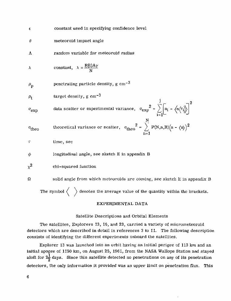
constant used in specifying confidence level

meteoroid impact angle

random variable for meteoroid radius

constant ,

penetrating particle density, g

target density, g j b-l

L

data scatter o r experimental variance, oexp 2 = 1 f - + ~ i $ j i=l

N theoretical variance or scatter, utheo = 2 P(N,n,R)(n - (n))2

n= 1

t ime, sec

longitudinal angle, see sketch E in appendix B

chi-squared function

solid angle from which meteoroids are coming, see sketch E in appendix B

The symbol ( ) denotes the average value of the quantity within the brackets.

EXPERIMENTAL DATA

Satellite Descriptions and Orbital Elements

The satellites, Explorers 13, 16, and 23, carried a variety of micrometeoroid detectors which are described in detail in references 3 to 11. The following description consists of identifying the different experiments onboard the satellites.

Explorer 13 was launched into an orbit having an initial perigee of 113 km and an initial apogee of 1150 km, on August 25, 1961, from the NASA Wallops Station and stayed aloft for 3 days. Since this satellite detected no penetrations on any of its penetration

detectors, the only information it provided was an upper limit on penetration flux. This

1

6

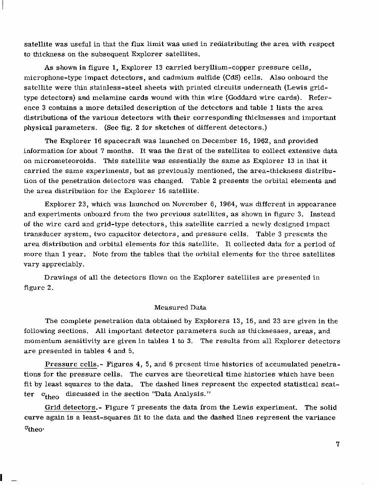
satellite was useful in that the f l u x limit was used in redistributing the area with respect to thickness on the subsequent Explorer satellites.

As shown in figure 1, Explorer 13 carried beryllium-copper pressure cells, microphone-type impact detectors, and cadmium sulfide (CdS) cells. Also onboard the satellite were thin stainless-steel sheets with printed circuits underneath (Lewis grid- type detectors) and melamine cards wound with thin wire (Goddard wire cards). Refer- ence 3 contains a more detailed description of the detectors and table 1 lists the area distributions of the various detectors with their corresponding thicknesses and important physical parameters. (See fig. 2 for sketches of different detectors.)

The Explorer 16 spacecraft was launched on December 16, 1962, and provided information for about 7 months. It w a s the first of the satellites to collect extensive data on micrometeoroids. This satellite was essentially the same as Explorer 13 in that it carried the same experiments, but as previously mentioned, the area-thickness distribu- tion of the penetration detectors was changed. Table 2 presents the orbital elements and the area distribution for the Explorer 16 satellite.

Explorer 23, which was launched on November 6, 1964, was different in appearance and experiments onboard from the two previous satellites, as shown in figure 3. Instead of the wire card and grid-type detectors, this satellite carried a newly designed impact transducer system, two capacitor detectors, and pressure cells. Table 3 presents the area distribution and orbital elements for this satellite. It collected data for a period of more than 1 year. Note from the tables that the orbital elements for the three satellites vary appreciably.

Drawings of all the detectors flown on the Explorer satellites are presented i n figure 2.

Measured Data

The complete penetration data obtained by Explorers 13, 16, and 23 a r e given in the following sections. All important detector parameters such as thicknesses, areas, and momentum sensitivity are given in tables 1 to 3. The results from all Explorer detectors are presented in tables 4 and 5.

Pressure cells.- Figures 4, 5, and 6 present time histories of accumulated penetra- tions for the pressure cells. The curves are theoretical time histories which have been f i t by least squares to the data. The dashed lines represent the expected statistical scat-

ter Otheo discussed in the section 'Data Analysis."

Grid detectors.- Figure 7 presents the data from the Lewis experiment. The solid curve again is a least-squares fit to the data and the dashed lines represent the variance

Otheo.

7

Wire cards.- The Goddard wire card data are presented in figure 8. Since only one penetration event was recorded on each set of cards, the theoretical curve was made to go through that one event for each thickness.

Impact detectors.- The events recorded by the impact detectors (figs. 9 and 10) are not considered to be impact data in this paper. It is thought that the detectors were ther- mally sensitive and that most events were caused by thermal effects. A complete dis- cussion of these effects is presented in a subsequent section.

Cadmium sulfide cells.- The Explorer 16 cadmium sulfide cell data (fig. 11) a r e not a histogram in the sense that the abrupt increases in hole area did not occur on the dates shown. The plot actually shows the hole area at the times when the satellite was in a proper position relative to the sun to enable a correct measurement to be taken. The CdS cells on Explorer 23 were ruptured during launch.

Explorer capacitor detectors.- Figure 12 presents the data from the capacitors onboard Explorer 23. Only two events were recorded by this detector and the theoretical curve is a straight line in this case. In the Data Analysis section it will be shown that the straight line reflects the fact that the sensitive area of the capacitors remains constant. The dashed lines represent the expected statistical scatter.

Pegasus capacitor detectors.- Table 6 presents the orbital elements and the data obtained with the Pegasus capacitor detectors. The Pegasus data are used later to con- struct a meteoroid model and are tabulated here for convenience.

DATA ANALYSIS

This section presents the analysis performed on the data. The analysis is com- posed of two main parts. The first part treats the satellite data as a se t of statistical events and examines relations between different detectors. The second part attempts to deduce information about the meteoroid environment from the data.

One-Shot Detectors

In experiments which consist of a number of one-shot detectors (detectors such as the pressure cells, the grid-type detectors, o r the wire cards flown on the Explorer pene- tration satellites), the time at which the ith cell was punctured is known. The total num- ber of particles which penetrated the entire area is not known since only the first particle to penetrate each cell is detected. The following statistical technique gives the time history of the number of punctured cells and is general enough to make possible extensive analysis of one-shot phenomena.

8

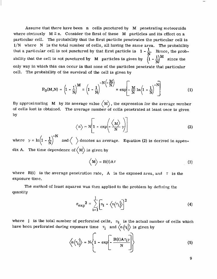
Assume that there have been n cells punctured by M penetrating meteoroids where obviously M 2 n. Consider the first of these M particles and its effect on a particular cell. The probability that the first particle penetrates the particular cell is 1/N where N is the total number of cells, all having the same area. The probability that a particular cell is not punctured by that first particle is 1 - -. 1 Hence, the prob-

ability that the cell is not punctured by M particles is given by (1 - i)M since the

only way in which this can occur is that none of the particles penetrate that particular cell. The probability of the survival of the cell is given by

N

By approximating M by its average value (M) , the expression for the average number of cells lost is obtained. The average number of cells penetrated at least once is given

where y = In ( 1 - $IN and ( ) denotes an average. Equation (2) is derived in appen-

dix A. The time dependence of

(M) = R(t)AT (3)

where R(t) is the average penetration rate, A is the exposed area, and T is the exposure time.

The method of least squares was then applied to the problem by defining the quantity

where j is the total number of perforated cells, ni is the actual number of cells which have been perforated during exposure time 7i and

9

which is obtained by substituting equation (3) into equation (2). The value of R(t) chosen was that value for which aexp2 was a minimum and, therefore, that value R(t) for which the following equation holds:

This procedure was followed on all the penetration data from the pressure cells and wire cards, and the results obtained are given in tables 4 and 5 and illustrated in figure 13.

The technique had to be modified for the grid-detector data since all the detectors were not of the same size. In this case, the number of cells not surviving is given by

J

where Ag,o and Ag,l are the respective detector areas and Ng,O and Ng,l are the respective numbers of detectors. Thus, equation (7) replaces equation (5) in the least- squares analysis for the grid-detector data.

Multiple-Event Detectors

Multiple-event detectors are capable of sustaining more than one impact or pene- tration event without the loss of the individual detector. The detectors falling into this category are the capacitor detectors, the CdS cells, and the impact detectors.

Capacitor detectors.- The capacitor detector is assumed to count all meteoroids passing through the outside steel sheet. Thus the number of detections 1 ( ~ ) at time T

is the same as the number of penetrating particles, namely,

" .~ .

1(T) = R(t)AcT = M 0 where A, is the total area of the capacitor detectors. Note that it is the reusable quality of the capacitor detectors which makes the number of detections equal to the num- ber of penetrating particles. The value of flux was determined by a least-squares fit of the calculated number of detections to the actual number of detections as was done with the pressure cells.

CdS cells.- The objective of the CdS experiment was to obtain some idea of the size of the micrometeoroids penetrating 6 p m of aluminized plastic film. This was done by

10

monitoring the resistance of a cadmium sulfide cell illuminated by sunlight coming in through the holes left by micrometeoroids. The data and a complete description of this experiment are reported in reference 7.

The analysis presented here attempts to deduce the size and the number of particles which penetrated the cadmium sulfide cell. The following assumptions were made in the analysis :

(1) The particles which penetrated the cells are characterized by an average size.

(2) According to reference 7, hypervelocity tests on this detector indicated that the hole diameter is 1.0 to 1.5 times greater than the particle diameter. The hole area is assumed herein to be 1.5 times the cross-sectional area of the particle.

In accordance with the assumptions, the total hole area Ah caused by M pene- trating particles all of {a) average radius is

Ah = 1.5M7r(a)

and the average penetration rate is

R(t) = - M ACdS '

where ACdS is the area exposed to the environment

(10)

for time 7. Since there are two equations and three unknowns, unique values for these unknowns cannot be obtained. The most information which can be obtained is a relation which summarizes all compatible values for two of the unknowns if some bound can be found for the other unknown. This analysis will attempt to put bounds on the number of penetrating particles by requiring that the data obtained from each of the two independent cells be consistent with one another.

As shown in figure 11, the ratio of the cumulative hole areas of one detector with respect to the other was about 3.4:l for an exposure time of about 22 days. If all the penetrating particles make holes of about the same size in the plastic film, the number of particles penetrating each cell should be in about the same ratio as the hole areas. Since the cells are identical, each cell should detect approximately the same number of parti- cles if the number of particles is reasonably large. This statement cannot be made if the number of particles is small, because in that case, it is very possible that one detec- tor will collect considerably more holes than the other. For example, if the detectors a r e identical, the probability that one detector will have three holes and the other six is much greater than the probability that one detector will have 300 holes and the other 600.

11

The ratio of the number of particles detected by the cells therefore implies something about the total number of particles.

The probability that m particles penetrate one of the two identical detectors and that M - m particles penetrate the other detector is

The probability of obtaining a ratio equal to or larger than 3.4:l is given by

P m' 2 3.4(M c where m' is the integer closest to the inequality. Thus the probability

0.77M and is obtained by solving the lower limit of of obtaining the present ratio or one larger is given

by equation (12). Figure 14 presents the value of this probability as a function of total number of penetrating particles M. It is seen that M is rather unlikely to be greater than 20.

Table 4 presents the relation between the penetration rate and the particle radius obtained by substituting the value for M from equation (9) into equation (10); an equation in terms of the product of the average particle size and penetration rate is thus obtained.

Impact detectors.- ~. -~~ No analysis is given here for the impact detectors since they are thought to produce spurious counts as a result of thermal effects. The matter is dis- cussed in Results and Discussion.

Conversion Factors

Tables 4, 5, and 6 give the penetration rates for the various experiments as func- tions of the detector thickness or sensitivity. A simple comparison of ra tes between the experiments is not physically meaningful since the penetration rates must be given as functions of a common detector and material combination, This section will interpret all the data in terms of an equivalent thickness of a stainless-steel pressure cell. The penetration data from all the Explorer detectors are shown in figure 13 in terms of an equivalent thickness of stainless steel.

Conversion of the data from the Lewis grid detectors and the beryllium-copper pressure cells to equivalent stainless-steel pressure-cell data proceeds very simply. The grid-type detector used stainless steel and like the pressure cell was sensitive to spalling; therefore, this material-detector combination is approximately the same as a pressure cell of stainless steel of the same thickness. The beryllium-copper pressure

12

cells, on the other hand, require a conversion constant to compensate for the differences in density of the two materials. The equation used for the conversion was the Fish- Summers penetration relation (ref. 12) which has a (&)-'I2 dependence on target den- sity. Tables 4 and 5 give the equivalent stainless-steel pressure-cell thicknesses for all the detectors onboard the Explorers.

An accurate analysis cannot be given for the Goddard wire-card data since not enough events were recorded to deduce the conversion constant empirically from the penetration data. However, since a particle causing a hole of radius equal to the wire diameter would probably break the circuit and since this same particle would probably also puncture a pressure cell of thickness equal to the wire diameter, it was assumed that copper wire cards were equivalent to stainless-steel pressure cells having a thick- ness equal to the wire diameter. The melamine backing which tended to increase the resistance to penetration on the detector compared with a pressure cell was assumed to be counterbalanced by the lower mass per unit area of the wire sheet which tended to decrease its penetration resistance.

An empirical conversion had to be performed for the stainless-steel capacitor data from Explorer 23 since no laboratory calibrations between stainless-steel capacitors and stainless-steel pressure cells were available. The low number of penetrations precluded a direct evaluation of the equivalent thickness of the capacitor detector in terms of stainless-steel pressure cells from the penetration data. The approach used to convert the stainless-steel capacitor data to stainless-steel pressure-cell data was to use the relation in equation (33) for conversion of a Pegasus aluminum capacitor thickness to an equivalent stainless-steel pressure-cell thickness, where the numerical value of the con- version constant q is 0.99. Since the Explorer capacitor detector material was stain- less steel instead of aluminum, the steel capacitor thickness first had to be converted to an equivalent aluminum capacitor thickness by use of the Fish-Summers penetration rela- tion (ref. 12). Then this aluminum capacitor thickness was converted to a stainless-steel pressure-cell thickness by using equation (33), with the value of q equal to 0.99.

E r r o r Analysis

Assuming that the penetrations were characterized by a Poisson distribution, the probability of M penetrations would be

P(M) = LR(t)Ad exp ER(t)Ad M!

The average flux would have a probability of 1 - E (ref. 4) of being within the bounds

13

where x2 is the chi-squared distribution function and Bi is the cumulative area-time product.

In order to calculate the upper and lower limits, Bi must be computed. It can be computed directly from the data, but will be calculated in another manner. By using equation (2) for the number of cells penetrated, an expression for the number of cells surviving at time T may be formulated:

and, therefore, the total area-time product is

where A is the total cell area and N is the number of cells. Substituting the value for Bi obtained in equation (16) into the limits (14) yields the limits

where ni has been approximated by n(Ti). The upper and lower limits on the penetra- tion rate given in tables 4, 5, and 6 were obtained by substituting the rate obtained by the least-squares technique into the limits in expression (17) and picking the confidence coef- ficient 1 - E to be 0.90.

The foregoing error analysis implicitly assumes that the penetration rate is con- stant, and this assumption was checked in the following manner: If the actual penetration rate were constant over the experimental area, data scatter would be expected since some particles would penetrate dead cells. This scatter is given by the variance

'the0 -

(n - (n))'P(N,n,(R)) = P P ( 1 - P j 1'2 n=O

14

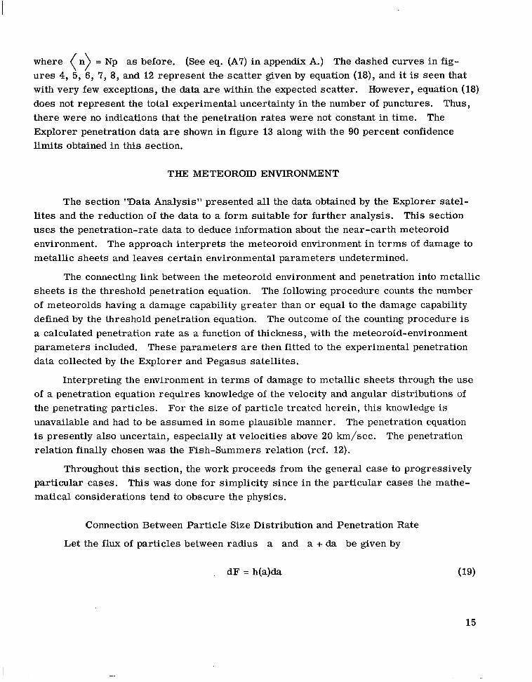
where (n) = Np as before. (See eq. (A?) in appendix A.) The dashed curves in fig- ures 4, 5, 6, ?, 8, and 12 represent the scatter given by equation (18), and it is seen that with very few exceptions, the data are within the expected scatter. However, equation (18) does not represent the total experimental uncertainty in the number of punctures. Thus, there were no indications that the penetration rates were not constant in time. The Explorer penetration data are shown in figure 13 along with the 90 percent confidence limits obtained in this section.

THE METEOROID ENVIRONMENT

The section 'Data Analysis" presented all the data obtained by the Explorer satel- lites and the reduction of the data to a form suitable for further analysis. This section uses the penetration-rate data to deduce information about the near-earth meteoroid environment. The approach interprets the meteoroid environment in terms of damage to metallic sheets and leaves certain environmental parameters undetermined.

The connecting link between the meteoroid environment and penetration into metallic sheets is the threshold penetration equation. The following procedure counts the number of meteoroids having a damage capability greater than or equal to the damage capability defined by the threshold penetration equation. The outcome of the counting procedure is a calculated penetration rate as a function of thickness, with the meteoroid-environment parameters included. These parameters are then fitted to the experimental penetration data collected by the Explorer and Pegasus satellites.

Interpreting the environment in terms of damage to metallic sheets through the use of a penetration equation requires knowledge of the velocity and angular distributions of the penetrating particles. For the size of particle treated herein, this knowledge is unavailable and had to be assumed in some plausible manner. The penetration equation is presently also uncertain, especially at velocities above 20 km/sec. The penetration relation finally chosen was the Fish-Summers relation (ref. 12).

Throughout this section, the work proceeds from the general case to progressively particular cases. This was done for simplicity since in the particular cases the mathe- matical considerations tend to obscure the physics.

Connection Between Particle Size Distribution and Penetration Rate

Let the f l u x of particles between radius a and a + da be given by

d F = h(a)da (19)

15

If these particles number of particles R

impinge on a unit surface of material T and thickness t, the penetrating this surface is given by

where gv and go are probability density functions (assumed statistically independent)

of the particle velocity v and impact angle 8. The integration is to be carried out over all appropriate values of the variables.

In order to f i x limits on the integration, a penetration equation is required. The threshold penetration equation is assumed to be of the form

- = f v COS 8,pp,T) a where f is a function, a is the particle radius, and t is the maximum thickness which can be penetrated by a particle of velocity v, impact angle 8, and density pp. The dependence on material thickness parameters is indicated by T.

Several investigators of hypervelocity impact in the past :(refs. 12 to 16) described their results in the form given by equation (21). Note that penetration has been assumed to depend on the normal component of velocity. ~

The integration in equation (20) is usually carried out over all values of the vari- ables. Thus the penetration rate R(t) is usually given by

where v1 and vo a r e the upper and lower limits of the velocity probability density function. Since penetration has been assumed to depend on mal to the plate, a simpler way of writing equation (22) is

where u is defined as the normal velocity component (u =

the velocity component nor-

du (2 3)

v cos 8) and gu(u) is the probability density function for this normal velocity component. This density function can of course be constructed from the density functions for impact angle and velocity. The limits of integration in equation (23) may be represented graphically as shown in sketch A. It is seen that i f a particle has a radius ap and a normal velocity up which

16

Particle radius

a

0 ;

Sketch A

are above the curve t = af u,p ,T , then the function apf(up,pp,T) is greater than the threshold penetration thickness t, and that particle will penetrate thickness t. From sketch A it is seen that the particles which wil l penetrate thickness t are those parti- cles which have radii and normal velocities in the shaded region because the function af(u,pp,T) is greater than t for those particles.

( P )

If a lower limit on particle size is assumed to be ao, the limits of integration in sketch A must be modified as shown in sketch B.

Particle radius

a

aO

t =

to be used in 4 equation (24)

I YS (t 5 to) region \ I

Equation (24) to be used in this region (t 2 to)

and for the lower curve,

where f'l is the inverse of the function f and T refers to the material dependence. The first equation is recognized as the integral commonly used for this problem - it is the same as equation (23) - but equation (24) is of a different character. It gives the thickness dependence for small thicknesses and describes the manner in which the pene- tration rate approaches its maximum value as a function of decreasing thickness. Equa- tion (25) is affected by the size cutoff, whereas equation (24) is not. The transition curve depicts the points where equations (24) and (25) give identical results. For thicknesses greater than to, equation (24) must be used, and for thicknesses less than to, equa- tion (25) must be used. By including a cutoff parameter in the analysis of penetration experiments, a particle population which substantially agrees with the zodiacal-light analysis of Beard (ref. 17) can be obtained.

Derivation of Penetration Rate for a Special Case

In accordance with meteor (ref. 18) and zodiacal-light results (ref. l?), the cumu- lative flux for a special case is given by

where F(a) is the cumulative flux of particles of radius a and greater, and P ( A > a) is the probability that the particle radius A is greater than the number a. More. cor- rectly, A is the random variable for particle radius and is used to denote the event that the particle radius is greater than a. Reference 19 may be consulted for more details about random variables. The penetration equation assumed is a more specific form of equation (21) which has been widely used in the past to describe results of hypervelocity experiments (refs. 12 to 15). The equation is given by

- = C(T)u pp t P 6 a

where p and 6 are material constants and C(T) is a constant which contains all the material properties of the target.

To obtain the penetration rate given in equations (24) and (25), the probability den- sity of the normal velocity is required. The probability density function for the normal

18

component of the impact velocity was obtained by assuming an isotropic f lux in the vicin- ity of the earth. Appendix B presents an argument for obtaining the probability density for impact angle. This density is given by the equation

The normal-velocity probability density function is obtained from the velocity prob- ability density and the impact-angle density in appendix C. The probability density for normal velocity is given by

where u is the normal velocity (u = v cos e), gv(v) is the velocity probability density, v1 is the upper limit of meteoroid velocities, and vo is the lower limit.

Once the function gu(u) has been computed, all the quantities necessary for eval- uating equations (24) and (25) have been compiled. The evaluation of the integrals in equations (24) and (25) is presented in detail in appendix D. It was found that the integra- tion gave different mathematical forms for penetration rate as a function of thickness. The expressions for penetration rate are given in equations (30), (3l) , and (32).

For 0 5 t 5 aoC(T)vo P d pp ,

R(t) = Fop - Kt2/P) (30)

where

19

For thicknesses simply

greater than or equal to aoC(T)vl@Pp6 = to, the penetration rate is

R(t) = Fo ( T l OLppu6aOo! (u"> t'" (32)

This last expression is the one which is usually used in interpreting penetration data and is interesting since it shows that the population index a! specifies the dependence of penetration rate on thickness of material provided that the material penetrated is rela- tively thick.

Cutoff Model

One way to determine the strength of cutoff effects is to try to fit a flux-mass model like the one given by equation (26) to the penetration data to see whether such a model can explain the data. Such a model is characterized by a cutoff and a constant slope on log- log scales.

The data available for the construction of the meteoroid model consist of the Explorer 16 and 23 pressure-cell results (tables 4 and 5) and the Pegasus capacitor- type-detector measurements (table 6).

In order to fit a particle f lux model from the satellite data, the penetration measure- ments must first be correlated since the Explorer and Pegasus satellites used different detectors and different materials. The assumption used here is that the Explorer stainless-steel pressure-cell thickness and the Pegasus aluminum-capacitor thickness are related by the equation

tE = q tp (33)

where tE represents the Explorer stainless-steel pressure-cell thickness, tp repre- sents the Pegasus aluminum-capacitor thickness, and q is a "total" conversion constant.

It should be noted in passing that the requirements necessary for equation (33) to hold are fairly flexible. If the penetration equation is given by

t = z(T)r a,v,6,pp 0 (34)

where z(T) is a function depending only on detector characteristics such as detector density, strength, and so forth, and r(a,v,6,pp) is a function depending only on the par- ticle parameters of size, velocity, impact angle, and density, then equation (33) holds. This happens because the Explorer penetration equation would be given by

20

tE = ~E(TE)r(a,v,e,Pp)

and the Pegasus penetration equation would be

Also, the ratio

(3 5)

is a constant depending only on the detectors, if the detectors are penetrated by the same particles. The penetration flux expected on the thicknesses tE and tp above is the same if they a r e exposed to the same environment. Two thicknesses related in the man- ner of equation (37) are said to be equivalent.

The penetration data used for fitting were the Explorer pressure-cell data and the 200 p m and 400 pm Pegasus data. The data from the thinnest Pegasus detectors were not used because the aluminum alloy used for these detectors was different from the alloy on the thicker detectors. Also, the thickness of the epoxy backing on the aluminum increased the resistance of this detector to penetration.

It was assumed that the Pegasus data were in the region where equation (32) holds, and thus a is the magnitude of slope of the Pegasus data and is given by

1

where R p is the Pegasus penetration rate. Since the slope for the Explorer data is less than for the Pegasus data, the Explorer data have to be in the region where equa- tions (30) and (31) hold. The values of FO and a0 are constrained to be consistent with these data since everything else in the expression is fixed once a velocity probability density and a penetration equation are chosen.

Since the velocity probability density function is not known for small particles, it must be assumed. The guidelines for assuming the density function were that it approx- imate meteor velocity density functions and that it be mathematically simple. The assumed density function is shown in figure 15 along with some meteor density functions (refs. 20 and 21) and is given by

21

The normal velocity probability density obtained by using equation (29) is derived in appendix C and is given by ‘

(0 5 u 5 11 km/sec) 7

The penetration equation used was the empirical Fish-Summers relation (ref. 12) given by

t - 1.82 ”- a p

where pt is the target density. This equation, obviously a specific form of equation (27), was used because it was derived from penetration into material sheets of finite thickness instead of the usual semi-infinite results. This equation implicitly assumes a particle density of about 2.7 g cm-3.

As previously mentioned the values of a0 and Fo were chosen to be consistent with the Explorer penetration data. The particular values for Fo and a0 were obtained by requiring equations (30) and (31) to give the actual penetration rates observed. These constants were obtained by trial and e r r o r and a r e given in the following table together with all the quantities used in the equations:

Fo, mm2 sec- l . . . . . . . . . . . . . . . . . . . . . . . . . . . . . . . . . . 6.7 x 10-6

a 0 , p m . . . . . . . . . . . . . . . . . . . . . . . . . . . . . . . . . . . . . . . . . . 5

(v-2), (sec/m)2. . . . . . . . . . . . . . . . . . . . . . . . . . . . . . . . . 3.0 x 10-3

Q . . . . . . . . . . . . . . . . . . . . . . . . . . . . . . . . . . . . . . . . . . . . . 2.1 p . . . . . . . . . . . . . . . . . . . . . . . . . . . . . . . . . . . . . . . . . . . . . 1.0

(,-Up>, (prn1-2 . . . . . . . . . . . . . . . . . . . . . . . . . . . . . . . . 2.0 x 10-7

q . . . . . . . . . . . . . . . . . . . . . . . . . . . . . . . . . . . . . . . . . . . . . o . g g

The choice of values for a0 and Fo determines the values for equations (30) to (32)

provided that the thickness t refers to an Explorer-type penetration detector. Because

22

of this the expression cannot be expected to fit the Pegasus data points for the two larger thicknesses since they have not been converted to Explorer thicknesses. To convert the Pegasus aluminum capacitor thicknesses to Explorer stainless-steel pressure-cell thick- nesses, the value of q in equation (33) must be determined. This value was obtained by determining the stainless-steel pressure-cell thicknesses corresponding to the Pegasus penetration rates. The thicknesses obtained in this manner are equivalent thicknesses. Knowing the equivalent thicknesses and the actual thicknesses is sufficient to calculate the value of q, which was determined as 0.99.

The meteoroid environment suggested by the present'investigation and other inves- tigations (refs. 10, 11, 17, 18, and 22) is given in figure 16. The flux for large particles was determined from meteor measurements (ref. 18) and extrapolated to the point where the curve intersected with the extrapolated curve from the present investigation.

RESULTS AND DISCUSSION

Statistical Analysis

One-shot detectors.- As previously mentioned, the results of analyzing all the one- shot detectors on the Explorer 16 and 23 satel l i tes are a se t of penetration rates with their respective limits (tables 4 and 5). The statistical analysis contains a number of more general results. One such result is the expression for the expected puncture time history given by equation (2). This equation clearly shows that the dependence of cells punctured on penetrating particles is an exponential function.

Another general result is the manner in which the predicted time history was f i t to the data. An important characteristic of the expressions developed and of the fitting tech- nique is that the entire technique can be used i f the penetration rate varies with time. This fact is important for meteoroid penetration experiments to detect time-varying pen- etration rates, such as a penetration rate measured in the asteroid belt. The penetration rate in that case would be dependent on the location of the satellite and the location of the trajectory of the satellite; these a re a function of elapsed mission time.

Multiple-event detectors. - Multiple-event detectors are capable of sustaining more than one impact or penetration without the loss of the individual detector. Impact detec- tors, cadmium sulfide cells, and capacitor detectors fall into this class.

-

Impact detectors: One of the objectives of the Explorer satellite series was the correlation of impact-detector data with penetration-type data. This was the reason for both types of experiments on one satellite. The threshold momentum levels of the detec- to rs were fixed so that a correlation of the two types of data would be possible. Thus it was expected that penetration rates and impact rates would be of the same order of

23

magnitude. Such was not the case, however, since the impact rates were generally much higher than the penetration rates (tables 4 and 5), and in some cases the rates differed by several orders of magnitude.

There have been doubts cast on the validity of measurements obtained by this type of detector. Nilsson (ref. 23) has found impact detectors on the OGO satellite& to be tem- perature sensitive, and the high impact rates obtained by the Explorer 23 satellite prompted Holden and Beswick (ref. 9, pp. 45-57) to investigate a possible temperature effect on the impact detectors onboard Explorer 23. Holden and Beswick's comparison of percent time in sunlight with impact rate is shown in figure 10 for Explorer 23. Figure 9 presents the same correlation for Explorer 16. Both figures show that when the satel- lites were in sunlight 100 percent of their orbit, the impact rates dropped rather drasti- cally. It should be noted that when the satellites were in sunlight 100 percent of the time, the satellite temperature was constant with time.

Probable causes of the behavior of the detector might be

(1) Piezoelectric elements can generate impact-type signals due to discontinuities in polarization as a function of temperature (ref. 24).

(2) Mechanical noise may also be generated by expansion and contraction of the sounding boards as a result temperature changes.

All the foregoing phenomena suggest that the impact data obtained by the Explorer satellites may in fact not be due solely to particle impacts but due also to various types of thermally caused system noise. Because the particle impacts apparently cannot be filtered from the thermally generated noise, the impact data from the Explorer satellites must be discarded. It should be noted, however, that this noise apparently depends on the threshold sensitivity of the system, and thus, the lowest-sensitivity impact detector on Explorer 23 may have obtained good data.

CdS cells: Table 4 presents all compatible values of the product of penetration rate and the square of the average particle radius for particles penetrating the cadmium sulfide detector. Also, statistical considerations of the data imply that the total number of pen- etrating particles was likely less than 20. If the value of penetration rate obtained from 20 penetrations in 22 days (5.1 X 10-3 m-2 sec-1) is substituted into the equation in table 4, the value of the average particle radius turns out to be about 16 pm assuming that the hole size is 1.5 times the projected area of the particle. The value for the penetration rate is about 3 orders of magnitude higher than the .penetration rate from the penetration measurements for particles of about the same size. Thus the penetration meaiurements and the CdS cell results seem to disagree. In an analysis of the same data (ref. 7), it was concluded that the CdS cell results were consistent with the f l u x model presented by

24

Alexander et al. (ref. 25), which predicted a great number (=1000) of penetrations through these detectors.

Capacitor detector: Although this detector sustained only two penetrations, it was considered a successful experiment. At the time of the flight it was felt that the elec- trons in the Van Allen belts would be trapped in the capacitor dielectric and that the capacitor would fire when the electron charge built up high enough to break down the dielectric. This effect was thought capable of causing false penetration events ranging in the hundreds. Reference 9 cites the capacitor data as inconclusive because it was impossible to determine whether the events were caused by meteoroid penetration or radiation effects. The approach taken here is to assume that the events were caused by meteoroid penetration and then to compare these measurements with all the penetration data to see whether the assumption is contradicted. It is seen in figure 13 that the two capacitor-detector events are compatible with the rest of the penetration data.

Error analysis.- The results of the error analysis, for example, the penetration- rate measurements, are given in tables 4, 5, and 6 and a r e shown as boundaries in fig- ure 13. More general results may be obtained by investigating how rapidly penetration rate goes to its ultimate value.

In order to see how fast the penetration rate converges, the value of penetration rate for the pressure cells given in table 5 was assumed to be the actual one and the limits (expression (17)) were interpreted to mean that experimental measurements should be within the limits given as a function of n. The resu l t s a re shown in figures 17 and 18.

This error analysis may be used to answer the question of how many punctures or events are necessary in order to have a good estimate of penetration rate. This is shown in figure 19 as the values of

These functions give the ratio of the confidence limits (expression (17)) to the actual value of penetration rate R, assuming y 1 (large number of cells) and therefore indicate how these limits converge to their ultimate value. It is seen that knowledge of penetra- tion rate goes from an upper bound at n = 0 to within a factor of 2 at n = 5.

Thus it is seen that most information about a constant penetration rate is obtained from the first few penetration events. The ratio of the upper and lower limits of penetra- tion rate to the actual penetration rate obtained is shown in figure 19. The ratio rapidly approaches 1 for about the first eight or 10 punctures. The "knee" of the curves occurs at about five punctures, and further significant closing of the confidence limits requires

25

many more punctures. For example, the probability is 80 percent that the penetration- rate estimate obtained from 30 punctures is between 1.25 and 0.77 times the actual pene- tration rate. On the other hand, the penetration-rate estimate for five punctures is between 1.8 and 0.48 times the actual penetration rate. It is readily seen that a sixfold increase in number of punctures does not give a penetration-rate estimate that is six times as good. It is also readily seen from the plot that sizable increases in accuracy accompany rather small changes in the number of punctures so long as the number of punctures is less than about eight or 10. Thus, most of the accuracy of the penetration rate is obtained from the first eight o r 10 punctures, and therefore, the minimum number of punctures yielding a "good" penetration-rate estimate is about eight or 10.

The penetration data failed to show the presence of shower effects in two ways:

1. The scatter from the expected or mean number of cells not surviving is with very few exceptions less than the average mathematical scatter Otheo expected from mete- oroids puncturing dead cells.

2. A convincing simultaneous increase in penetration rates for two or more detec- tors or detector thicknesses was not observed.

Thus, it was concluded that the shower component of the meteoroid environment could not be distinguished from the sporadic component.

Penetration Data and the Meteoroid Environment

Equations (30), (3 l), and (32) clearly show that a curved line for penetration rate against thickness can be expected on log-log scales even though the flux as a function of particle radius is a straight line. Sketch C illustrates the situation.

c

log FO a-@ dependence

log penetration

rate

"-,_c""- "" :_

log particle radius log thickness

Sketch C

26

The fitting of the penetration data to a distribution function of the zodiacal-light type has given a simple explanation for the difference in slope between the Explorer and Pegasus data. The explanation is that the slope change is due to cutoff effects. The model obtained by fitting the penetration data to a meteoroid model with a cutoff is shown in figure 16 along with other meteoroid models for comparison. There are, of course, other explanations for the slope difference.

One possible explanation for the slope differences between Pegasus and Explorer data is that the cumulative flux as a function of thickness is curved on log-log scales. As mentioned previously, this possibility was investigated by Naumann (ref. 11) and Alvarez (ref. 10). Each investigator fitted a curved cumulative flux function to the Explorer and Pegasus data and each found that his respective model predicted a cutoff. Both cutoff predictions were close enough to the data so that cutoff effects were to be expected. Had cutoff effects been incorporated in the functions, the flux curve would have been closer to a straight line. These investigators did not t ry all functions which produce a curved cumulative flux function, and it is also possible that the flux function looks as depicted in sketch D.

Other possible population functions

log flux .-Naumann (ref. 11) and Alvarez (ref. 10) type predictions

L . . ._ ". "

log particle radius

Sketch D

The flux function can, of course, have just about any shape provided that the cumulative flux never decreases with decreasing radius.

Another explanation for the slope difference is that the penetration equation is not of the form given by equation (21). For example, if the penetration equation is nonlinear and is given by

27

(43)

where T again refers to target parameters and w is a function, there is in general no reason to expect the Pegasus and Explorer data to define the same slope even if the flux function is a straight line. One way of avoiding difficulties like this is to calibrate the detector by determinibg the mass or s ize of the particle required to penetrate it at mete- oroid velocities. The penetration rate through the material is then equated to the f l u x corresponding to that mass. In order for the calibration procedure to yield valid results, the detectors in space have to be thick enough so that there are no cutoff effects. There is at present no way to determine whether the particles penetrating the Explorer detectors a r e far enough away from cutoff to permit a valid calibration.

The foregoing remarks show the need for an experiment to determine cutoff. Such an experiment does not require much area; for example, a penetration detector a few micrometers thick with an area of about 0 .5 m2 would suffice to test the validity of cut- off models like the present one.

Since experiments on small thicknesses give little information on the form of the flux function and those on large thicknesses do, it becomes obvious that another pene- tration detector thicker than the Pegasus detectors might indicate the manner in which penetration experiments and meteor measurements are tied together. Such an experi- ment would surely be indicative of the rate of change of slope, if any. It should be noted, however, that i f cutoff is determined experimentally to be very much higher than about 7 x 10-6 m-2 sec-1 - a doubtful possibility since the Explorer slopes are so flat - then Explorer and Pegasus measurements would indeed imply that the exponent Q defined in equation (38) is not constant. <

CONCLUDING REMARKS

A probability analysis of the one-shot detectors onboard the Explorer 13, 16, and 23 satellites showed that the puncture time history could be adequately represented by an exponential of the form n = N ( 1 - FAT) where n is the number of cells punctured during exposure time T, N is the initial number of detectors, and X is a constant. This exponential expression resulted from the loss of detectors with time. No unexpected deviation from this formula was noted in the data, thus, a constant penetration rate was indicated. Shower effects could not be detected in the data. The technique used to deter- mine the penetration rate is also flexible enough to be used when the penetration rate is time dependent rather than constant with time.

The meteoroid data from Explorers 13, 16, and 23 were analyzed statistically and were found to show a good degree of consistency with the exception of the data from the

piezoelectric impact detector and the cadmium sulfide cell. The impact-detector data were probably not due solely to meteoroid impacts but also to temperature effects both on the piezoelectric crystal and on the detector structure. Because of this, the impact data were not included in the meteoroid analysis. The cadmium sulfide cell data tended to disagree with the penetration data and, furthermore, seemed to exhibit a degree of self-inconsistency if the number of penetrating particles was assumed to be large. As a result, the analysis of the CdS cell data was termed inconclusive.

Analysis of the convergence rate of penetration rate as a function of number of detections indicated that most knowledge is obtained by the first eight or so detections. The convergence of constant flux after eight detections becomes a slowly varying function of number of detections.

The penetration data from both the Explorer and Pegasus satellite series were examined and it was found that a variety of flux-mass models can explain these data. A model of the environment of the form used in zodiacal-light work was hypothesized and fit to the data as a test of the strength of cutoff effects. The model was found capable of accounting for the penetration data obtained thus far and, furthermore, seems also to agree with zodiacal-light results. The model obtained for small particles is given by

F(a) =

c where F(a) is the flux of particles having radius a or larger, Fo is the maximum flux observable and equal to about 7 km-2 sec-1, and the cutoff radius a0 is about 5 pm. The radius at which the flux from the satellite data intersects with results from ground- based meteor measurements is 0.9 mm.

The analysis performed indicates that the parameter most urgently needed now is the cutoff flux Fo. An empirical value for the cutoff would indicate the shape of the f l u x as a function of particle dimensions. An experiment such as this does not need a large exposed area.

Langley Research Center, National Aeronautics and Space Administration,

Langley Station, Hampton, Va., November 24, 1969.

29

APPENDIX A

DERIVATION OF' TIME HISTORY OF PUNCTURED CELLS

The probability obtained in equation (1) is a conditional probability since it assumes that M particles have penetrated the cells. Then, a suitable value for M must be obtained in the derivation of the time history of punctured cells. If the probability of obtaining M penetrations were known, the probability of survival of the cell would be given by

where Ps is the survival probability, Po is the conditional probability that any one cell will survive M penetrating meteoroids, and P(M) is the probability of M pene- trations. An average value for PS would next be obtained as follows:

where ( ) indicates an average value. If P(M) were known, the average value of P,

could be obtained, but in reality P(M) is unknown, and an alternate approach must be chosen. The approach chosen here is simply that an average value such as that described by equation (A2) yields a number close to Po((M) ,N) and the approximation used herein is that

= exp(- + 3 -N

where y = ln(l - i) . Note that the survival probability is a function of the average

number of penetrating particles per cell - (M) and a constant y (which is close to 1) N

provided that the initial number of one-shot detectors is reasonably large.

30

APPENDIX A

The probability that the detector was punctured at least once is therefore

Since the detector was picked qt random, equation (A4) is true of any detector and hence the probability that n out of N cells will be penetrated is given by the binomial distribution

where

and p is given by equation (A4).

The average number of cells

- N

(') = n!(N - n)! N!

penetrated is given by 7

Thus the expected time history has the form of an exponential.

31

APPENDIX B

IMPACT-ANGLE PROBABILITY DENSITY FUNCTION

The number of particles per second passing through an elemental area dA and coming from the solid angle dS2 (in steradians) is given by

where G(B,+) is the number of particles sec-1 m-2 sr-1 coming from direction e,+ as is shown in sketch E.

Z

Sketch E

The direction of the normal to dA also defines the Z-axis.

The f lux is given by

and the assumption of isotropic flux implies that G(8,+) is a constant. The probability density was obtained by dividing the flux by G(8,+) and normalizing over a hemisphere. Therefore, the impact-angle probability density function is given by

go( e) = 2 sin e cos e = -2 COS e - COS e d de

32

APPENDIX C

NORMAL-VELOCITY PROBABILITY DENSITY FUNCTION

The normal-velocity probability density function was obtained from the velocity probability density and the impact-angle density, as shown in this appendix. The prob- ability that the normal velocity (u = v cos e) is equal to or l e s s than u is given by P(U 5 u), which is the probability that the normal velocity random variable U is equal to or less than the number u. This probability requires that U be in the shaded por- tion of sketch F:

"""""

"I 1 I u = v COS e

COS e I

VO "

Particle velocity v V 1

Sketch F

The expression for this probability is

P(U 5 u) = { "

The density function for u, where u = v cos 8, is obtained by differentiating the prob- ability with respect to u and is given by

33

APPENDIX C

gu(u) = - P(U 5 u) = d du

34

APPENDIX D

RELATION BETWEEN PENETRATION FLUX AND PROBABILITY DENSITY FUNCTIONS

In performing the integrations in equations (24) and (25), it was found necessary to segment the regions of integration since these different regions give different forms to the penetration rate. Sketch G illustrates the three thickness ranges where the penetra- tion rate has radically different dependences on thickness.

Particle radius

a

-For all particles in 4 cross-hatched region,

0 - - I 1

u = vo u = v1

Particle normal velocity u

Sketch G

It will be shown that for thicknesses less than to, the penetration rate varies as

Fo(l - Kt2/p), and thus as t goes to zero, the penetration rate goes to FO as expected.

For thicknesses greater than t l (particles in region In), the penetration rate will be shown to vary as t-@, also as expected. ’ Thicknesses in the range between t l and to a r e i n a transition region and the penetration rate is not easily expressible as a function of thickness.

The particles in the cross-hatched area starting in region I are those particles for which the normal velocities u and radii a are such that C(T)auPpppb 2 t and thus those particles capable of penetrating thickness t provided t 5 to. Thus in region I where 0 5 t 5 aOC(T)vo@ppb = to,

35

Substituting equation (D2) in place of the probability distribution in equation (Dl) gives

The number density may be expressed as

by differentiating equation (26) where gA(a) is the probability density for particle size

and is defined as -gA(a) = - P(A > a). Thus equation (D3) may now be expressed as d da

The asymptotic dependence on thickness for very small thicknesses is therefore

R(t) = Fo (1 - Kt2/$

36

APPENDIX D

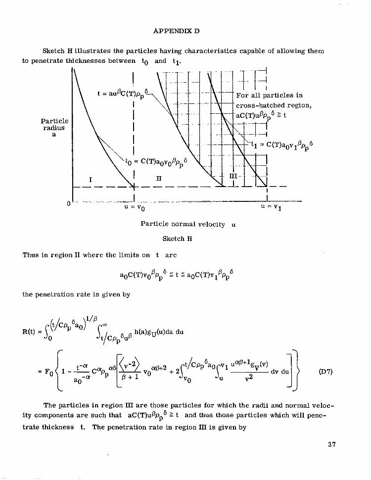
Sketch H illustrates the particles having characteristics capable of allowing them to penetrate thicknesses between to and tl.

Particle radius

a

V u = vo u = v1

Particle normal velocity u

Sketch H

Thus in region 11 where the limits on t a r e

the penetration rate is given by

The particles in region 111 are those particles for which the radii and normal veloc- ity components are such that aC(T)uPpp6 2 t and thus those particles which will pene-

trate thickness t. The penetration rate in region 111 is given by

37

APPENDIX D

38

REFERENCES

1. D'Aiutolo, Charles T., coordinator: The Micrometeoroid Satellite Explorer xIII (1961 Chi) - Collected Papers on Design and Performance. NASA TN D-2468, 196.4.

2. Hastings, Earl C., Jr., compiler: The Explorer X V I Micrometeoroid Satellite - Description and Preliminary Results for the Period December 16, 1962, Through January 13, 1963. NASA TM X-810, 1963.

3. Hastings, Earl C., Jr., compiler: The Explorer XVI Micrometeoroid Satellite - Supplement 1, Preliminary Results for the Period January 14, 1963, Through March 2 , 1963. NASA TM X-824, 1963.

4. Hastings, Earl C., Jr., compiler: The Explorer XVI Micrometeoroid Satellite - Supplement 11, Preliminary Results for the Period March 3, 1963, Through May 26, 1963. NASA TM X-899, 1963.

5. Hastings, Earl C., Jr., compiler: The Explorer XVI Micrometeoroid Satellite - Supplement 111, Preliminary Results for the Period May 27, 1963, Through July 22, 1963. NASA TM X-949, 1964.

6. Davison, Elmer H.; and Winslow, Paul C., Jr.: Micrometeoroid Satellite (Explorer XVI) Stainless-Steel Penetration Rate Experiment. NASA TN D-2445, 1964.

7. Secretan, Luc: Measurements of Interplanetary Dust Particle Flux From Explorer XVI CdS and Wire Grid Dust Particle Detectors. GSFC X-613-66-451, NASA, Sept. 1966.

8. O'Neal, Robert L., compiler: The Explorer XXIII Micrometeoroid Satellite - Description and Preliminary Results for the Period November 6, 1964, Through February 15, 1965. NASA TM X-1123, 1965.

9. O'Neal, Robert L., compiler: The Explorer XXIII Micrometeoroid Satellite - Description and Results for the Period November 6, 1964, Through November 5, 1965. NASA TN D-4284, 1968.

10. Alvarez, Jose M.: Satellite Measurements of Particles Causing Zodiacal Light. The Zodiacal Light and the Interplanetary Medium, J. L. Weinberg, ed., NASA SP-150, 1967, pp. 123-129.

11. Naumann, Robert J.: The Near-Earth Meteoroid Environment. NASA TN D-3717, 1966.

39

12. Fish, Richard H.; and Summers, James L. : The Effect of Material Properties on Threshold Penetration. Proceedings of the Seventh Hypervelocity Impact Sympo- sium, vol. VI ( A D 463 232), Feb. 1965, pp. 1-26. (Sponsored by U.S. Army, U.S. Air Force, and U.S. Navy.)

13. Charters, A. C.; and Locke, G. S., Jr.: A Preliminary Investigation of High-speed Impact: The Penetration of Small Spheres Into Thick Copper Targets. NACA RM A58B26, 1958.

14. Anderson, G. D.: Studies in Hypervelocity Impact. Poulter Lab. Tech. Rep. 018-58, Dec. 1959.

15. Walsh, J. M.; and Johnson, W. E.: On the Theory of Hypervelocity Impact. Pro- ceedings of the Seventh Hypervelocity Impact Symposium, vol. 11 ( A D 463 228), Feb. 1965, pp. 1-75. (Sponsored by U.S. Army, U.S. Air Force, and U.S. Navy.)

16. Herrmann, Walter; and Jones, Arfan H.: Correlation of Hypervelocity Impact Data. Proceedings of the Fifth Symposium on Hypervelocity Impact, vol. 1, pt. 2 ( A D 284 280), Apr. 1962, pp. 389-438. (Sponsored by U.S. Navy, U.S. Army, and U.S. Air Force.)

17. Beard, David B.: Interplanetary Dust Distribution. Astrophy. J., vol. 129, no. 2, Mar. 1959, pp. 496-506.

18. Whipple, Fred L.: Meteoroids and Dust. Bioastronautics and the Exploration of Space, Theodore C. Bedwell, Jr., and Hubertus Strughold, eds., Dec. 1965, pp. 7-24. (Sponsored by Aerosp. Med. Div., U.S. Air Force.)

19. Feller, William: An Introduction to Probability Theory and Its Applications. Vol. II, John Wiley & Sons, Inc., c.1966, pp. 165-217.

20. Clough, Nester; and Lieblein, Seymour: Significance of Photographic Meteor Data in the Design of Meteoroid Protection for Large Space Vehicles. NASA TN D-2958, 1965.

21. Dohnanyi, J. S . : Model Distribution of Photographic Meteors. TR-66-340-1 (Contract NASw-417), Bellcomm, Inc., Mar. 29, 1966.

22. Van de Hulst, H. C.: Zodiacal Light in the Solar Corona. Astrophys. J., vol. 105, no. 3, May 1947, pp. 471-488.

23. Nilsson, Carl: Some Doubts About the Earth's Dust Cloud. Science, vol. 153, no. 3741, Sept. 9, 1966, pp. 1242-1246.

24. Kittel, Charles: Introduction to Solid State Physics. Second ed., John Wiley & Sons, Inc., 1963, p. 186.

40

25. Alexander, W. M.; McCracken, C. W.; Secretan, L.; and Berg, 0. E.: Review of Direct Measurements of Interplanetary Dust From Satellites and Probes. Space Research III, Wolfgang Priester, ed., North-Holland Pub. Co. (Amsterdam), 1963, pp. 891-917.

41

TABLE 1.- EXPLORER 13 DETECTOR PROPERTIES AND ORBITAL ELEMENTS

Detector

Langley pressure cells

~

Lewis grid detectors

Goddard wire cards

Langley impact detectors

Goddard CdS cells

-L

date, August 25, 1961. Initial orbital elements: apogee, 1150 km; perigee, 113 km; inclination, 37.7O- period, 97 min 1

1 p m 1 dyne-sec 1 cm2 1 Of 1 detectors Thickness, Sensitivity, detector, Area per Number Total initial

Material

Annealed beryllium- copper throughout; density, 8.23 g cm-3 ~ 51

I

i \ 40 3940

I I I 20 i 1970 I

i 64 I

\' i 20 1970 I 127 \ I 20 1970

, Stainless steel, type 1 76 1 1 58.1 j 50 2905

!

I 304, throughout; 1 152 i

density, 7.83 g cmm3 ' 58.1 ~ 10 581 ~

I i I

I 7. r"---i-i

Copper wire wound on I a51 44 l4 I 616

melamine card

Lead zirconate

16 j 1408 ~

88 a76

2 I 1420 , 709 0.01 I

titanate piezo-

Aluminized plastic 40

2 1420 709 1.0 electric element 20 1 1970 98.5 .1

I

aWire diameter. bThickness of aluminized plastic film.

TABLE 2.- EXPLORER 16 DETECTOR PROPERTIES AND ORBITAL ELEMENTS

Detector

Langley pressure cells

Lewis grid detectors

Goddard wire cards

Langley impact detectors

Goddard CdS cell

date, December 16, 1962. Initial orbital apogee, 1180 km; perigee, 750 km; inclination, 52O; period, 104 min

Material Thickness, Pm

Annealed beryllium- copper throughout; density, 8.23 g cm-3

Stainless steel, type 304, throughout; density, 7.83 g cm-3

Copper wire wound on melamine card

Lead zirconate titanate piezo- electric element

Aluminized plastic film

25 51

12 7

25 25 76 76

152

a51 a76

b6

aWire diameter. bThickness of aluminized plastic film.

dyne-brc~I deteOcftars Sensitivity, detector, area,

cm2

Area per Number Total initial

98.5

I 116 58.1

116 58.1 58.1

44

~ 88

100

1970 20 3940 40 98 50

8 928 8 464 8 928

15 232 4 8 72

14 6 16 16 1408

0.1 .5

1.0

709 98.5

70 9

2

1420 2 19 70 20 1420

1 2 0 1 2 1 40

2

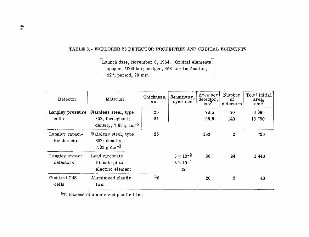
TABLE 3.- EXPLORER 23 DETECTOR PROPERTIES AND ORBITAL ELEMENTS

[Launch date, November 6, 1964. Orbital elements4 I apogee, 1000 km; perigee, 458 km; inclination, I I 52O; period, 99 min - i

Detector Material

Langley pressure 302, throughout; cells

Stainless steel, type

density, 7.83 g cm-3

Thickness, I-lm

25 51

Sensitivity, dyne-sec

Langley capaci- Stainless steel, type 25 tor detector 302; density,

7.83 g cm-3

Area per of detector,

Number

cm2 detectors

Total initial area, cm2

6 895 13 790

363 2 72 6

Langley impact Lead zirconate 3 x 10-2 60 24 1 440 -~

detectors titanate piezo- 8 x 10-1 electric element 12

Goddard CdS Aluminized plastic “6 20 2 40 cells film

aThickness of aluminized plastic film.

TABLE 4.- EXPLORER 16 RESULTS

(a) Penetration detectors

Thickness of Total Penetration rate, m-2 sec-l Unshielded penetration Thickness, equivalent number rate limits, m-2 sec-1

cell, pm events Upper Lower Detector

Pm steel pressure Of Earth shielded Unshielded "

Langley pressure 3.9 x 5.2 x 6.6 x 10-6 3.9 x 10-6 ' cells 2.0 x 2.7 x 10-6 4.4 x 1.4 x 10-6

12 7 0 1.2 x 10-6

Lewis grid 25 6 4.7 X 10-6 6.3 X 10-6 1.2 X 10-5 3.4 X 10-6 I 3.3 X 10-7 detectors 76 1

8.7 X 10-7 1.2 X loe6 1 3.0 X 152 152 0 1 1.6 X 10-5 0

Goddard wire a5 1 1 8.8 X 10-7 3.0 X 10-8 2.8 X 10-6 5.8 X 10-7 cards a76 75 1 4.3 X 10-7 6.2 X loW8 5.7 X 10-6 1.2 X "} Assumed

I

Goddard CdS b6 cells I

awlre diameter. bThickness of aluminized plastic film.

(b) Langley impact detectors

Sensitivity, Impact rate, m-2 sec-1

dyne-sec Earth shielded , Unshielded

0.1 4.0 X 10-3 3 X 10-3 .5 1.3 x 10-2 10-2 i 1.0 2.0 X 10-3 1.5 X 10-3

TABLE 5.- EXPLORER 23 RESULTS

(a) Penetration detectors

Langley pressure 25 51

Thickness of equivalent

steel p res su re cell, pm events

25 51 74 2.5 x 10-6

"I

Langley capaci- 25 43 (Calculated) 2 8.8 x 10-7 tor detector I

~~ ~ _.

Goddard CdS "6 Rupture of plastic film during take-off rendered CdS cells inoperative cells

I

"Thickness of aluminized plastic film.

(b) Langley impact detectors

Sensitivity, Impact rate, m-2 sec-1

4.8 X 10-4 7.0 X 10-4 12 4.4 X 10-7 6.4 X 10-7

TABLE 6.- PEGASUS ORBITAL ELEMENTS AND RESULTS

(a) Orbital elements

rr- Launch date

Pegasus 3 July 30, 1965

I I

744 496 31.8 1 1 748 506 31.8 97

540 52 1 28.9 95

(b) Results

Aluminum Equivalent steel capacitor

thickness, thickness, pressure-ce.11

I.lm I-lm

Unshielded Number

m-2 sec-l events rate, of penetration

Penetration rate limits (90% confidence),

m-2 sec-1

r v E i 3.16 x 10-6 i 3.38 x 10-6 i 2.94 x 10-6 I I 400 1 400 1 201 1 8.17 x I 9.15 x I 7.19 x 1

Impact CdS c e l l t r a n d u c e r s

Be-Cu p r e s s u r e c e l l s

It

ewi s pr i d- / t y p e d e t e c t o r s

Goddard w i r e c a r d s

Figure 1.- Photograph of Explorer 13. L-61-2274.1

48

0.30

A a A

B

Stainless-steel test material

Section A-A

2.46

(a) Langley pressure-cell detector (Explorers

Figure 2.- Sketches of detect01

.i

13, 16, and 23).

's on Explorers 13, 16, and 23. (Al l

on inside 8 p a i n t e d b l a c k on o u t s i d e < T h e r m i s t o r

(b) Gcddard CdS cell (Explorers 13 and 16).

dimensions are in centimeters unless labeled otherwise.)

m 0

11.61

rr / - , - - 7 6 o r 1 5 2 pm s ta in less s tee l cover

25 pm p las t ic insu la to r

1.52 p m th ick go ld g r id

813 pm thick si l icone rubber

panels 72 -7

11' 30'

I I i

26.35

I I LO. 13 thick plate

(c) Lewis grid detector (Explorers 13 and 16). (d) Langley impact detector (Explorer 23).

Figure 2.- Continued.

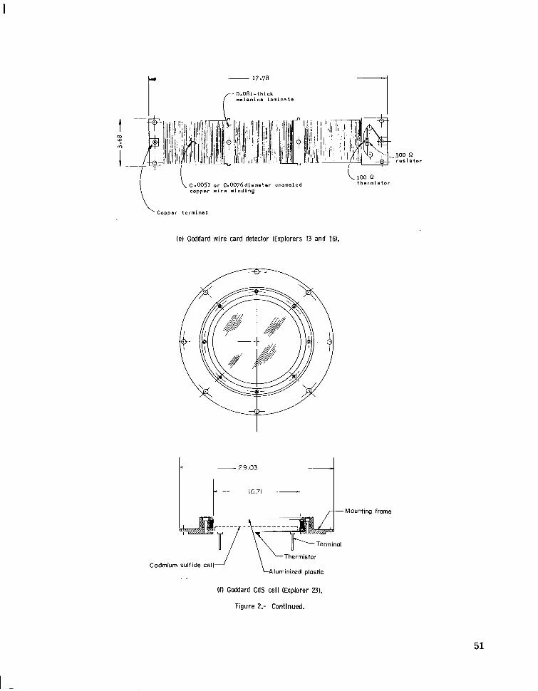
I- 17.78 1 0.081-thick melamine laminate

\ 100 n 0.0051 o r 0.0076diamster enameled copper w i r e winding

thermistor

Copper terminal

(e) Goddard wire card detector (Explorers 13 and 16).

1 1 - ~ 29.03

I I I A Mountina frame

LThermistor

Aluminized plastic Cadmium sulfide cell

(f) Goddard CdS cell (Explorer 23).

Figure 2.- Continued.

51

Nose- cone skin

- Piezoelectric crystal -- -.

Section A - A

.OQ7 e lec t r i ca l inference shield

.~ .~

(g) Langley impact detector (Explorers 13 and 16).

Fiber-glass mounting board

fl

Thermistor

"

- I

-.

J

__

t- i

0.63 open foam 7_

~ Printed circuit

(h) Langley capacitor detector (Explorer 23).

Figure 2.- Concluded.

52

Figure 3.- Photograph of Explorer 23. L-64-10,894.1

53

Days in o r b i t

Figure 4.- Explorer 16 beryllium-copper pressure-cell data.

50

.- C

Days i n o r b i t

Figure 6.- Explorer 23 stainless-steel pressure-cell data. Detector thickness, 50 pm.

0 20 40 6 0 80 100 12 0 140 16 0 180 200

Days i n o r b i t

Figure 7.- Explorer 16 Lewis (stainless-steel) grid-type detector data.

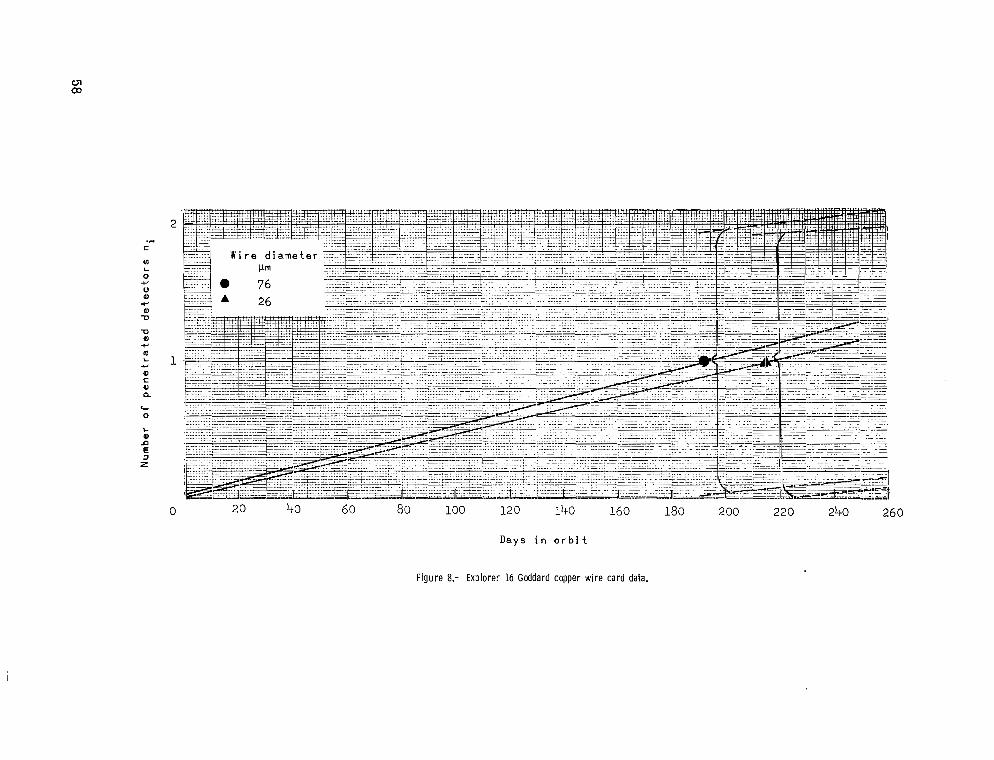
al c

n 0

rc 0

L

0 20 60 80 100 120 l ’ tO 160 180 200 220 240 260

Days i n o r b i t

Figure 8.- Explorer 16 Gcddard copper wire card data.

100

80

x

6 0 d

L 0) a u)

20

100 0

d y n e - s e c )

L 0 ) c a --

I I ._ " 1 6 0 .- I 1 1 I 0 20 40 60 a0 100 120 140

Days i n o r b i t

Figure 9.- Explorer 16 impact detector data. The high-sensitivity-system data are not shown because that system failed (ref. 5).

59

cn 0

x x

rb 7) rb

U

400 r

L Q C a .-

0 40 80 120 16 0 200 240 280 3 20

Days i n o r b i t

Figure 10.- Explorer 23 impact detector data (ref. 9).

.1

.O1

.oo:

.OOOl 0

I l l I I I

U 20

'Detector 1

30

r

40

Days i n o r b i t

60

I

Figure 11.- Explorer 16 cadmium sulfide cell data (ref. 7).

61

4- 0

L m n a E

z

0 20 40 60 80 100 120 l b O 160 180 200 220 240 260

Days i n o r b i t

Figure 12.- Explorer 23 capacitor detector data.

100 1000 10 000

Equivalent stainless-steel thickness,

Figure 13.- Comparison of satellite data with proposed model.

63

.20

.10

0 0 2 4 6 8 10 12 14 16 18 20

Total number o f penetrating particles M

Figure 14.- Results of cadmium sulfide cel l data analysis (eq. (12)).

.10

9 09

.08

[ v

.02 g

.Ol 1 0 --

1

+-

P r o b a b i l i t y d e n s i t y f u n c t i o n s

D o h n a n y i ( r e f . 21)

ttti+t+t c 1 o u g h a n d L i e b l e i n ( r e f . 2 0 ) N o r m a l - v e l o c i t y p r o b a b i l i t y

r e p r e s e n t a t i v e d e n s i t y

d e n s i t y

m w d e n s i t y o b t a i n e d f r o m

_ _ _ _ R e p r e s e n t a t i v e p r o b a b i l i t y

10

\'\

" -

V e l o c i t y v a n d n o r m a l v e l o c i t y c o m p o n e n t u, km/sec

Figure 15.- Velocity probability density functions.

65

II I II II I I I I I 1111 II II

lo-+

lo4

10-8

4

I 0 Q)

LL

/ ' N a u m a n n

Van d e H u l s t ( r e f . 22)

A l v a r e z ( r e f . 10)

P r e s e n t m o d e l

\\ \ r W h i p p l e ( r e f . 18)

l oo M e t e o r o i d mass, p

Figure 16.- Comparison of meteoroid models.

1 7 )

' \ I

lo2

66

lo4 8

6

4

2

10-5 8

6

4

2

10'6 8

6

4

2

10-7 8

6

4

2

10-8 0

i de nce

10 20 30

I /

I /

10% Confidence limits +

rate least-squar es

40

Number of cells punctured n i

50 60

Figure 17.- Comparison of actual convergence with convergence expected from Poisson statistics for the 25-pm thick detector on Explorer 23.

67

8

6

4

2

10-5 8

..

Y

2 10-6 c 8 n

Y

: 4 Q

2

10-7 8 6

4

2

10-8 0 10

% Confidence

20

1 imi ts

30 40

Confidence

(per imental le rnetration rat

Number of cells punctured ni

as e

i T

I

i

4 1 t

i i I

1 I

I I I

1 I I I I I j

i I I

1

limits # i I

50 60 70

Figure 18.- Comparison of actual convergence with convergence expected from Poisson statistics for the 5-pm thick detector on Explorer 23.

68

10.

8.

6.

4.

2.

1.

.8

m 6

.2

.1 .08

06

-04

.02

908 Ti dc

10

/

20

Number o f c e l l s p u n c t u r e d n i

Figure 19.- Convergence of penetration rate.

NASA-Langley, 1970 - 30 L-5944 69

NATIONAL AERONAUTICS AND SPACE ADMINISTRATION WASHINGTON, D. C. 20546

OFFICIAL BUSINESS FIRST CLASS MAIL

NATIONAL AERONAUTICS ANT POSTAGE AND FEES PAID

SPACE ADMINISTRATION

, :. '<'C.

. .

, >, , .1 , ': I I, '? , , ~ , , ; : "

! , , ! ' . !. " 1 1 I . . , . . .< , 7

POSTMASTER: If Undeliverable (Section 15s Postal Manual) Do Not Return

NASA SCIENTIFIC AND TECHNICAL PUBLICATIONS * .

TECHNICAL REPORTS: Scientific and technical information considered important,

' ' . complete, and a lasting contribution to existing . '. knowledge. 1..

TECHNICAL NOTES: Information less broad in scope but nevertheless of importance as a contribution to existing knowledge.

TECHNICAL MEMORANDUMS: Information receiving limited distribution because of preliminary data, security classifica- tion. or other reasons.

CONTRACTOR REPORTS: Scientific and technical information generated under a NASA contract or grant and considered an important contribution to existing knowledge.

TECHNICAL TRANSLATIONS: Information published in a foreign language considered to merit NASA distribution in English.

SPECIAL PUBLICATIONS: Information derived from or of value to NASA activities. Publications include conference proceedings, monographs, data compilations, handbooks, sourcebooks, and special bibliographies.

TECHNOLOGY UTILIZATION PUBLICATIONS: Information on technology used by NASA that may be of particular interest i n commercial and other non-aerospace application<. Publications include Tech Briefs, Ttchnology Utilimtion Reports and Notes, and Technology Surveys.

Details on the availability of these publications may be obtained from:

SCIENTIFIC AND TECHNICAL INFORMATION DIVISION

NATIONAL AERONAUTICS AND SPACE ADMINISTRATION Washington, D.C. 20546