Statistical Analysis of Dr. Guthrie

Public Reception of Dr. Guthrie

With General Discussion of Various Statistical Questions following the Report

By Scott Graham

Ma 405

5-5-15

Note: this is written for a technical audience (a math professor). While non-technical audiences are welcome to read this,

please understand there may be a large amount of undefined statistical vocabulary in this report.

2

Table of Contents

Abstract 5

Sample Characteristics 6

ANOVA 12

Regression 22

Contingency 26

General Discussion 28

Bibliography 32

3

Abstract

Procedures We did a study to test the public reception of a fictional soft drink, Dr. Guthrie (Dr. G). We had each recipient rate the taste of Dr. G on a Likert Scale of 1 to 5 and then had them compare it with Dr. Pepper (Dr. P) to see which they liked better. This will tell us how to market the soft drink. We then analyzed the data the above results and compared them to the demographics of our population. The specific independent demographics were Gender, Age, Minority Status, and Education Level. We used an ANOVA test to compare the means and see exactly which demographics were the most successful; Regression to predict the reaction of a male minority that is 39 years old with 13 years of education and to find out which factors were significant; a contingency study to see if taste and favor were dependent on certain factors.

Conclusions

ANOVA We should market primarily to elderly females in the minority. They seem to receive Dr. G better than the other demographics. The only demographic we should avoid in general is the Youth. They did not

receive Dr. G very well at all (taste=2.78 on a Likert Scale 1 to 5). The rest of the demographics received Dr. G fairly well. We could market to them and still get some profit. In competing with Dr. P, we should mainly worry about Age and Education Level. For Age, we will do better in the younger age groups. For education level, we will do better with those that have a high school education. While ANOVA shows that minority status does not make a difference in Favor, it does show that we will succeed over 50% of the time in advertising to non-minorities with 95% confidence.

Regression For Taste, we found that Education level is not significant in predicting a person’s enjoyment of Dr. G. We then came up with the following model to predict their rating on a Likert Scale of 1 to 5.

.0591.229 .913 .894gen age minTaste X X X

For Favor, we found that Gender and Minority Status were not significant in predicting whether or not a person liked Dr. G over Dr. P. We came up with the following model in which 1 means he will choose Dr. G and 0 means he will choose Dr. P.

. .022 .655068age edFavor X X

Contingency The only new thing Contingency told us is that at α=.05, we do not need to worry about Minority Status as a predictor of Taste. However, the other two tests said we should pay attention to minority status so I recommend we do pay attention to Minority Status.

4

Sample Characteristics To test the acceptance of Dr. Guthrie soft drink, we surveyed 50 people with varying ages, degrees of

education, genders, and ethnicities.

Gender Out of 50 people, 28 were women and 22 were men.

Ethnicity 16 of the sample were in the ethnic minority

34 were non-minorities

Gender

Men 44%

Women 56%

Percent Minorities

Non-minorities 68%

Minorities 32%

5

Ages The ages for the sample were distributed as seen below:

Age Frequency

Youth (0-19) 9

Young Adult (29-39) 24

Middle Aged (40-71) 17

Average Age: 33.2

0

10

20

30

40

50

60

Perc

ent

Age

Age Distribution

0 10 20 30 40 50 60 70 80

Age

Age Statistics Boxplot

6

Education Level The education level was only in number of years so I had to make some assumptions about the degrees

of education attained. I assumed the following for degrees of education:

Degree Years of Education Frequency in Sample

Elementary (k-6) 7 13

High School (7-12) 13 26

College/Grad 14+ 11

The education levels of the people in the sample are seen below:

0

10

20

30

40

50

60

Perc

ent

Education Degree

Education Distribution

7

0

5

10

15

20

25

30

35

40

Perc

ent

Taste (Likert Scale)

Distribution of Likert Ratings

Series1

2%

10%

20%

38% 30%

General Survey Results

Comparison with Dr. Pepper

Overall, the participants enjoyed Dr. Guthrie more than Dr. Pepper.

Likert Rating

Overall, Dr. G was well received by the participants. With 95% confidence, the data shows that Dr. G is

liked by the general public since the mean is greater than 3.

Mean 3.84

Standard Deviation 1.04

p-value for >3 3E-7

Preferred Soda

Dr. Pepper

36%

Dr. Guthrie

64%

8

Correlations Taste

Collinearity of Variables

Taste on Likert

Scale Gender Age Minority Status Education

Pearson

Correlation

Taste on Likert Scale 1.000 .411 .691 .274 .073

Gender .411 1.000 -.142 -.169 -.005

Age .691 -.142 1.000 -.050 .097

Minority Status .274 -.169 -.050 1.000 .106

Education .073 -.005 .097 .106 1.000

Sig.

(1-tailed)

Taste on Likert Scale . .002 .000 .027 .307

Gender .002 . .163 .120 .486

Age .000 .163 . .364 .251

Minority Status .027 .120 .364 . .232

Education .307 .486 .251 .232 .

From this, we see that the only dependent variable at α=.05 is Taste. The other variables are independent of each other.

Favor Collinearity

Favor Gender Age Minority Status Education

Pearson Correlation Favor 1.000 .091 -.590 -.111 .479

Gender .091 1.000 -.142 -.169 -.005

Age -.590 -.142 1.000 -.050 .097

Minority Status -.111 -.169 -.050 1.000 .106

Education .479 -.005 .097 .106 1.000

Sig. (1-tailed) Favor . .266 .000 .222 .000

Gender .266 . .163 .120 .486

Age .000 .163 . .364 .251

Minority Status .222 .120 .364 . .232

Education .000 .486 .251 .232 .

From this, we see that the only dependent variable is Favor at α=.05. The other variables are independent of each other.

9

ANOVA

Gender We found that on average, the females liked Dr. G more than the males. However, there was no difference in their preferences to Dr. G and Dr. P.

Taste

Descriptives

N Mean

95% Confidence Interval for Mean Sig Lower Bound Upper Bound

Male 22 3.36 2.86 3.87 .003 Female 28 4.21 3.91 4.52 Total 50 3.84 3.55 4.13

On average, the females gave Dr. G a rating .85 higher rating than the men on a Likert Scale 1 to 5.

H0: men=women

H1: men<women

p=.003<α=.05, ∴Reject H0.

From the data, we see that on average, females like Dr. G better than Dr. P.

Note: Homoscedasticity is not violated with p=.033<α-.05

Conclusion: We should market more to females than to males.

MenWomen0.0%

20.0%

40.0%

60.0%

Men

Women

Gender by Taste

10

Favor

N Mean

95% Confidence Interval for Mean Sig Lower Bound Upper Bound

Male 22 .59 .37 .81 .531

Female 28 .68 .49 .86 Total 50 .64 .50 .78

H0: men=women

H1 men<women

p=.531>α=.05 ∴Reject H0.

From the data, we see that on average, females like Dr. G better than Dr. P more than men do.

Note: Homoscedasticity is violated with p=.245>α=.05

Conclusion: We should not worry about gender when competing with Dr. P.

11

Age We found that enjoyment of Dr. G increases with age. However, the elderly prefer Dr. P over Dr. G more than the middle aged and youth. Therefore, we should market mostly to the elderly unless we will be competing directly with Dr. P.

Taste

Descriptives

N Mean

95% Confidence Interval for Mean

Lower Bound Upper Bound

Youth 9 2.78 2.14 3.42

Middle Aged 24 3.67 3.28 4.05

Elderly 17 4.65 4.34 4.96

Total 50 3.84 3.55 4.13

Scheffe Multiple Comparisons

(I) Age Grp (J) Age Grp Mean Difference (J-I) Sig.

Youth

Middle Aged

Middle Aged .889* .026

Elderly 1.869* .000

Elderly .980* .002

On average, the elderly gave Dr. G a rating .98 higher rating than the middle aged who gave it a

rating .89 higher than the youth on a Likert Scale of 1 to 5.

H0: Youth=Middle=Elderly

H1: Youth<Middle<Elderly

All p<α=.05, ∴Reject H0.

From the data, we see that on average, the elderly like Dr. G more than the middle aged which

likes Dr. G more than the youth.


Conclusion: We should market mostly to the elderly, some to the middle aged, and very little to

the youth. (Graph on next page).

12

Youth

Young AdultsMiddle Aged

0.0%

20.0%

40.0%

60.0%

80.0%

StrongDislike

Dislike Neutral LikeStrong

Like

Youth

Young Adults

Middle Aged

Age Group by Taste

13

0%

20%

40%

60%

80%

100%

Youth YoungAdults

MiddleAged

Dr. P

Dr. G

Age Group by Preference

Favor

Descriptives

N Mean



Youth 9 1.00 1.00 1.00

Middle Aged 24 .75 .56 .94

Elderly 17 .29 .05 .54

Total 50 .64 .50 .78

Scheffe Multiple Comparison

(I) Age Grp (J) Age Grp

Mean Difference

(I-J) Sig.

Youth

Middle Aged

Middle Aged .250 .311

Elderly .706* .001

Elderly .456* .005

On average, the females gave Dr. G a rating .85 higher rating than the men on a Likert Scale

H0: Youth=Middle=Elderly

H1: Youth>Middle>Elderly

PYM.31>α=.05, PYE=.001<α=.05, PME=.005<α=.05, ∴Reject H0.

From the data, we see that on average, there is no provable difference in the preferences of the

youth and middle aged. Both tend to prefer Dr. G. However, there is a difference between the

preferences of the elderly and the youth and middle aged. The elderly tend to prefer Dr. P more.

Note: Homoscedasticity not is violated with p=.0+>α=.05

Conclusion: In competing with Dr. P, we should not market to the elderly but more to the youth

and middle aged.

14

0%

10%

20%

30%

40%

50%

StrongDislike

Dislike Neutral LikeStrong

Like

Non Minorities

Minorities

Ethnicity by Taste

Minority Status We found that, on average, minorities like Dr. Guthrie more than non-minorities at α=.06. We can therefore market to minorities more than to non-minorities. However, it is safe to compete with Dr. Pepper in non-minorities but not in minorities.

Taste

Descriptives

N Mean


Sig. Lower Bound Upper Bound

Non-Minority 34 3.65 3.27 4.02 .054

Minority 16 4.25 3.79 4.71

Total 50 3.84 3.55 4.13

On average, the minorities gave Dr. G a rating .6 higher rating than the non-minorities on a Likert

Scale 1 to 5.

H0: minorities=non-minorities

H1: minorities>non-minorities

p=.054>α=.05, ∴Do not reject H0.

From the data, we see that on average there is not much of a provable difference between

minorities and non-minorities in their enjoyment of Dr. G.


Conclusion: We cannot reject H0 at α=.05. However, we can reject it at α=.06. That is still plenty

so we can still fairly safely market to minorities more than non-minorities.

15

Favor

Descriptives

N Mean


Sig Lower Bound Upper Bound

Non-Minority 34 .68 .51 .84 .444

Minority 16 .56 .29 .84

Total 50 .64 .50 .78

On average, the minorities gave Dr. G a rating .14 higher rating than the non-minorities on a Likert

Scale 1 to 5.

H0: minorities=non-minorities

H1: minorities<non-minorities

p=.444>α=.05, ∴Do not reject H0.

While there is no provable difference from the data in preference between minorities and non-

minorities, we can say with 95% confidence that most non-minorities prefer Dr. G while we cannot

say the same about minorities.


Conclusion: Avoid competing with Dr. Pepper for minorities but do not avoid non-minorities.

0%

10%

20%

30%

40%

50%

60%

70%

80%

90%

100%

Non-minority Minority

Dr. P

Dr. G

Ethnicity by Preference

16

0.0%

50.0%

Stro

ng…

Dis

like

Neu

tral

Like

Stro

ng

Like

Elementary

Secondary

Post-Secondary

Education by

Education According to the data, education level does not affect a person’s enjoyment of Dr. G. However, we found that those with a high school education tended to prefer Dr. G over Dr. P more than those with a Gradeschool or College education.

Taste

Descriptives

N Mean Std. Error



Gradeschool 16 3.81 .306 3.16 4.46

High School 17 3.88 .241 3.37 4.39

College/Grad 17 3.82 .231 3.33 4.31

Total 50 3.84 .147 3.55 4.13

Sheffe Multiple Comparisons

(I) Ed Grp (J) Ed Grp

Mean Difference

(J-I) Sig.

95% Confidence Interval


Gradeschool

High School

High School .070 .982 -1.00 .86

College/Grad .011 1.000 -.94 .92

College/Grad -.059 .987 -.86 .98

On average, the college/grad people gave Dr. G a rating .01 lower rating than the gradeschool

people who gave it a rating .05 lower than the high school on a Likert Scale of 1 to 5.

H0: Grades=High=College

H1: Grades <College<High

All p>α=.05, ∴Do not reject H0.

From the data, we see that on average,

education level makes no provable difference

a person’s enjoyment of Dr. G.

Note: Homoscedasticity is violated with

p=.434>α=.05

Conclusion: We should not look at education

level to find out who will enjoy Dr. G.

17

Favor

Descriptives

N Mean Std. Error



Gradeschool 16 .38 .125 .11 .64

High School 17 .53 .125 .26 .79

College/Grad 17 1.00 .000 1.00 1.00

Total 50 .64 .069 .50 .78

Scheffe Multiple Comparison

Multiple

Comparisons On average, the females gave Dr. G a rating .85 higher rating than the men on a Likert Scale

H0: Grades=High =College

H1: Grades <High<College

PGH=.57>α=.05, PGC=0+<α=.05, PHC=.007<α=.05, ∴Reject H0.

From the data, we see that on average, there is no provable difference in the preferences of the

gradeschool and high school groups. However, there is a difference between the preferences of

the college and the gradeschool and high school. The college group tends to prefer Dr. G. more.

Note: Homoscedasticity is not violated with p=.0+>α=.05

Conclusion: In competing with Dr. P, our time would be better spent advertising to those with a

college/grad level education. Advertising to lower education groups would be very risky.

(I) Ed Grp (J) Ed Grp

Mean Difference

(J-I) Sig.

95% Confidence Interval


Gradeschool

High School

High School .154 .565 -.52 .21

College/Grad .625* .000 -.99 -.26

College/Grad .471* .007 -.83 -.11

18

Regression From the data, we found that, in analyzing taste, Gender, Age, and Minority Status were all

significant factors in predicting a person’s enjoyment of Dr. G. Education, however, was not a

significant factor.

Also from the data, we found that only Age and Education were significant factors in a person’s

preference between Dr. P and Dr. G. Gender and Minority Status were not significant factors in

predicting a person’s favor.

Taste

Multiple Linear Regression

Coefficients with Significance

Model

Variable

Unstandardized

Coefficients

B Sig.

(Constant)

Gender (Xgen)

Age(Xage)

Minority Status(Xmin)

Education(Xed)

1.009

1.232

.060

.924

-.012

.000

Βgen .000

Βage .000

Βmin .000

Βed .312

From the data, we see that at α=.05, all of the above factors excluding education (pEd=.312>α) are

significant in the prediction of a test statistic’s taste

We believe we can to some degree predict how much a person will like Dr. G with the following

equation:

1.232 .012 1.0. 0906 .924

gen gen age age min min ed ed

gen age min ed

Taste X X X X k

X X X X

Example: a male minority that is 39 years old and has 13 years of education will, on average, give

Dr. Guthrie a rating of 4.12 on a Likert Scale 1 to 5.

Note: from the table of correlations, all of the variables above besides Taste are independent of

each other.

19

Stepwise Regression

R-Squares of Model

Model

R

Square

Adjusted R

Square

Age .477 .466

Age, Gender .742 .731

Age, Gender, Minority Status .908 .902

The Stepwise Regression did not include Education in its model. Therefore, we can eliminate that

from our model giving us:

gen gen age age min minTaste X X X k

Therefore, do not analyze education level in determining whether or not to advertise to them.

Here is another Regression model calculated without Minority:

Regression without Education

Model

Unstandardized

Coefficients

B Sig.

(Constant)

Gender

Age

Minority Status

.894 .000

1.229 .000

.059 .000

.913 .000

Here is the model we came up without Education.

.0591.229 .913 .894gen age minTaste X X X

Example: a male minority that is 39 years old and has 13 years of education will, on average, give

Dr. Guthrie a rating of 4.108 on a Likert Scale 1 to 5.

20

Favor

Multiple Linear Regression

Coefficients with Significance

Model

Unstandardized

Coefficients

B Sig.

(Constant)

Gender

Age

Minority Status

Education

.732 .000

-.035 .682

-.023 .000

-.216 .019

.071 .000

From the data, we see that at α=.05, all of the above factors excluding Gender (pgen=.682>α) and

Minority Status (pmin=.222>α) are significant in the prediction of a test statistic’s taste

We believe we can to some degree predict how much a person will like Dr. G with the following

equation:

.035 .023 – .0216 .071 .732

gen gen age age min min ed ed

gen age min ed

Favor X X X X k

X X X X

Example: a male minority that is 39 years old and has 13 years of education will, on average, favor

Dr. G 54.2% of the time.

Note: from the table of correlations, all of the variables above besides Taste are independent of

each other.

21

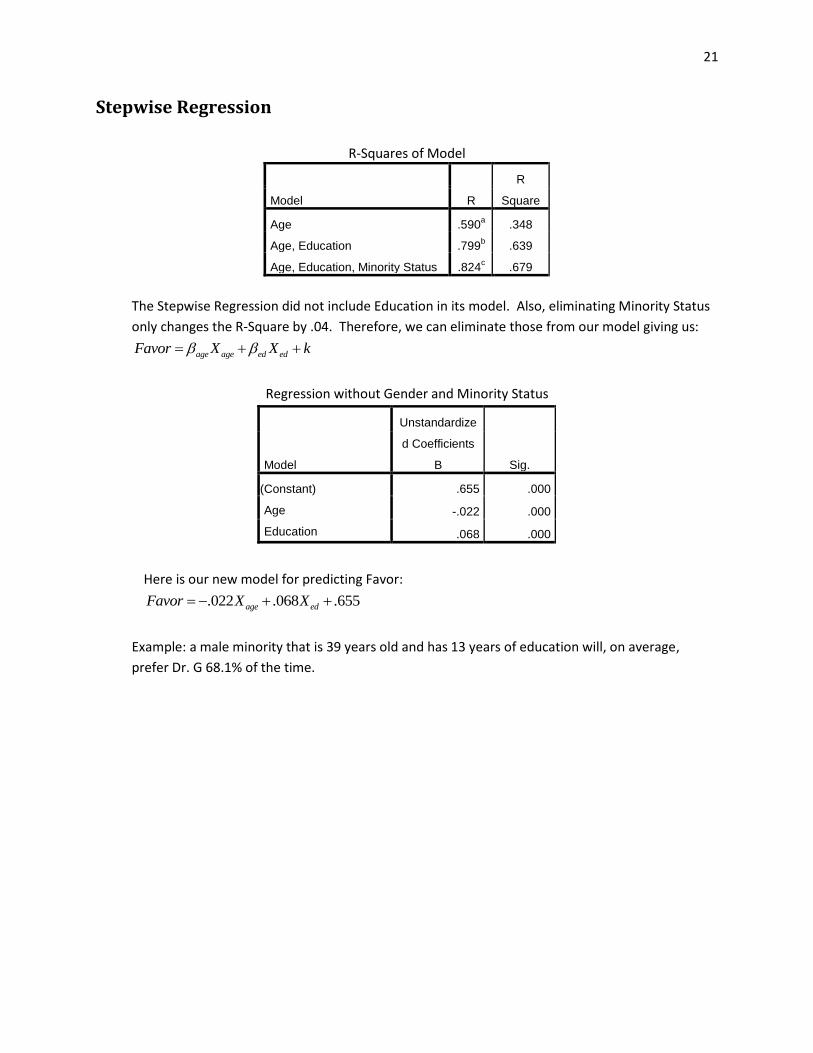
Stepwise Regression

R-Squares of Model

Model R

R

Square

Age .590a .348

Age, Education .799b .639

Age, Education, Minority Status .824c .679

The Stepwise Regression did not include Education in its model. Also, eliminating Minority Status

only changes the R-Square by .04. Therefore, we can eliminate those from our model giving us:

age age ed edFavor X X k

Regression without Gender and Minority Status

Model

Unstandardize

d Coefficients

B Sig.

(Constant)

Age

Education

.655 .000

-.022 .000

.068 .000

Here is our new model for predicting Favor:

. .022 .655068age edFavor X X

Example: a male minority that is 39 years old and has 13 years of education will, on average,

prefer Dr. G 68.1% of the time.

22

Contingency

Taste

Pearson Chi-Square

Phi Sig

Gender 11.30 .475 .023

Age 39.25 .888 .000

Education 4.413 .297 .818

Minority Status 4.713 .307 .318

According to this analysis, there is no significant difference in enjoyment of Dr. G between

difference in Education levels and Minority Status (α=.05). We should only study Age and Gender.

Favor

Pearson Chi-Square

Phi Sig

Gender .411 .091 .522

Age 15.150 .550 .001

Education 15.342 .554 .000

Minority Status .613 .111 .434

According to this analysis, there is no significant difference in enjoyment of Dr. G between

differences in Gender or Minority Status (α=.05). We should only study Age and Education.

23

General Discussion

I. Discuss the problem with the type I error in repeated t-test and how to

handle that problem by A. Bonferroni’s correction on Alpha

In hypothesis testing, pi=α is the probability that a Type I error will occur for a single

test, i. When n hypothesis tests are used, the probability of one Type 1 error is

approximately ip n . Therefore, to keep the actual p to a minimum, we must

divide α by n to get the correct p=α. For example, if we want 95% overall confidence for

five testes, we would have to use α=.01 for each individual test. This will give as an

overall α=.05.1

B. Multiple test as ANOVA and Regression.

ANOVA and Regression don’t need to be adjusted because they are, by definition, all

under the same α.2

II. For ANOVA A. Discuss the type of variables (dependent = performance and independent =

influencing)

In ANOVA, we study whether or not the performance of a variable is influenced by the

characteristics on another variable. For example, a person’s performance in grades may

be influenced by his gender. Another way to say this is his grades are dependent (to a

degree) on his gender. His gender is not dependent of any other variables in the test. It

is independent.3

B. Discuss the assumptions to do an ANOVA test.

1. Random Sample: if it is not a random sample, we could prove anything.

2. Dependent variable is normally distributed: The equation for an ANOVA uses a Normal

distribution.

3. Population Variances must be equal. This is required for the formula to work. Otherwise it

is very complicated.4

C. How would you handle ANOVA data that violated homoscedasticity?

First, make sure the violation is significant enough to worry about. Many times,

heteroscedasticity occurs because one mean is much larger than the other. Try using a

log transformation. Also, you can try to use a Welch’s ANOVA.5

1 Guthrie, Gary. "Intro for Final Project." Ma 405. United States, Greenville. 22 Apr. 2015. Lecture.

2 Abbey Young (paraphrasing Gary Guthrie)

3 Guthrie, Gary.

4 "Hypotheses Statements and Assumptions for One−Way ANOVA." Hypotheses Statements and Assumptions for

One−Way ANOVA. N.p., n.d. Web. 04 May 2015.

24

D. What is tested under ANOVA?

ANOVA tests the differences of means to see if they are significant.6 They are also

useful because they give us a measure of confidence as well.

E. How does one use the results of ANOVA to do confidence intervals for the average

score in a group? If one graphed all of the confidence intervals what would we like to

see?

Instead of using the t-distribution, we can use the F-distribution to find the critical

values of a sample.7 If we graphed the confidence intervals for multiple tests on the

same subject with unchanging factors, we would ideally like to see all of the confidence

intervals placed around the same area.

F. Discuss how to do ANOVA with regression

Since the coefficients in regression are the differences in means in ANOVA from a

reference variable, the p-values in regression give us the significance of the differences

in the means from the reference variable. The two are pretty much the same thing.

One analyzes the means, the other analyzes the difference in means.8

III. For regression A. Discuss the type of variables (dependent = performance and independent =

influencing)

This is the same as in ANOVA. The dependent variables are influenced by the

independent variables. The purpose of regression is to measure how much the

influence of the independent variables affects the performance of the dependent

variables.9

B. Discuss the assumptions to do a regression analysis.

1. For Linear, it there must be a linear relationship. The data sample points must form a

somewhat straight line. Same for Quadratic, Log, etc.

2. Multivariate Normality

3. Little or no multicolinearity: the independent variables may not influence each other in the

test.

4. No autocorrelation: residuals may not be independent from each other.

5. Homoscedasticity: the variances must be equal.10

5 McDonald, John H. "Handbook of Biological Statistics." Homoscedasticity -. N.p., 4 Dec. 2014. Web. 04 May 2015.

6 "Analysis of Variance (ANOVA)." Analysis of Variance (ANOVA). N.p., n.d. Web. 04 May 2015.

7 "Confidence Interval for ANOVA." Real Statistics Using Excel. N.p., n.d. Web. 05 May 2015.

8 Grace-Martin, Karen. "Why ANOVA and Linear Regression Are the Same Analysis." The Analysis Factor RSS. N.p.,

n.d. Web. 05 May 2015. 9 Guthrie, Gary

10 "Assumptions of Linear Regression - Statistics Solutions." Statistics Solutions. N.p., n.d. Web. 05 May 2015.

25

C. Discuss how each of the following can be used to analyze how good a regression

model fits

1. R2

R2 tells us how much of our dependent variable can be predicted by our independent

variables, on average. If R2 is .1, our model is predicting 10% of the dependent

variable.11

2. Residuals and sum of residuals squared

The residuals are simply individual differences between the observed data points and

the expected data points from the model. These typically cannot tell us very much as

some will be negative and some will be positive so their sum can be zero even if it is a

horrible fit. The sum of residuals squared, however will always be positive. It will tell us

how much residual we have in our prediction.12

3. 0 1: ... 0nH

We multiply the coefficients βi by the characteristics of or surrounding the test subjects.

If the coefficients are smaller, they will have less effect on the dependent variable. If we

cannot reject H0, the model is useless because the coefficients cannot predict the

dependent variable.13

D. Discuss how one does a parsimony study.

A parsimony goes through the different factors and analyzes them to see which ones are

useful in analyzing data and in constructing a model. One technique is using a stepwise

regression and seeing how much R2 each of the independent variables contains. If they

contain less than .05, we can disregard that factor as insignificant in our study. After

finding the useless factors, go through and do another regression study excluding the

rejected factors.

E. How does one use the results of regression to do confidence intervals for an

individual’s score that has certain demographic characteristics?

Regression Analysis in SPSS returns the standard error along with the confidence

interval. In this test, we want to see if any of the coefficients equal zero. If zero is in the

confidence interval, we can reject that demographic since it is insignificant.

IV. For contingency – give the questions and answers. A. What is a contingency table?

A contingency table (also known as a Cross Tab table) looks at the divisions within

groups of different factors and looks at how they are distributed across the dependent

discrete results. It can be done in counts, percent, or both. Note: if dealing with

11

"Goodness-of-Fit Statistics." Goodness of Fit Statistics. N.p., n.d. Web. 05 May 2015. 12

Guthrie, Gary 13

Guthrie, Gary

26

continuous data, break up the data into several ranges.14 For two variables Ai and Bi, a

2x2 contingency table looks like the following:

B1 B2 Total

A1 1 1A B 1 2A B

1An

A2 2 1A B 2 2A B

2An

Total 1Bn

2Bn 1 2 1 2A A B Bn n n n

B. Discuss the type of variables (dependent = performance and independent =

influencing)

The goal is to see whether or not the independent variables influence the dependent

variables. It does this by grouping the results into different categories. We can then

look at the resulting table to see if it looks like the variables are dependent and use it in

the calculation of the Chi-Square

C. Discuss Pearson’s Chi-Square.

The Pearson Chi-Square test is used to see if the variables are independent of each

other. It starts with the null hypothesis that the two variables are independent of each

other. Two variables A and B in the above table are independent if

1 2 1 2

i j

i j

A A B B

A BA B

n n n n

.

This is t called the expected value. The Chi-Square finds the sum of the squares of the

differences between each factor’s expected and observed values divided by the

expected value. The higher the Chi-Square, the more likely the variables are

independent. We then use the p-value for hypothesis testing to test the null

hypothesis.15

D. Explain Phi and Cramer’s V

Phi is simply a square root of a Chi-Squared divided by n. It is bounded by 0 and 1.0 and

tells us how predictable one variable is given another variable. Note: Phi is only good

for 2x2 contingency tables.

Cramer’s V is just like Phi except that it also divides by the smaller of (rows-1) or

(columns-1). Therefore, for a 2x2, Cramer’s V=Phi. However, it is useful because it will

not go above 1.0 for tables larger than 2X2. It tells us the same as Cramer’s V.16

14

Stockburger, David W. "Chi-Square and Tests of Contingency Tables." Chi-Square and Tests of Contingency Tables. N.p., n.d. Web. 05 May 2015. 15

"Pearson's Chi-Square Test for Independence." Upenn. N.p., n.d. Web. 05 May 2015. 16

"Nominal Association: Phi and Cramer's V." Measures of Nominal Level Association. N.p., n.d. Web. 05 May 2015.

27

Bibliography

"Analysis of Variance (ANOVA)." Analysis of Variance (ANOVA). N.p., n.d. Web. 04 May 2015.

"Assumptions of Linear Regression - Statistics Solutions." Statistics Solutions. N.p., n.d. Web. 05 May

2015.

"Confidence Interval for ANOVA." Real Statistics Using Excel. N.p., n.d. Web. 05 May 2015.

"Goodness-of-Fit Statistics." Goodness of Fit Statistics. N.p., n.d. Web. 05 May 2015.

Grace-Martin, Karen. "Why ANOVA and Linear Regression Are the Same Analysis." The Analysis Factor

RSS. N.p., n.d. Web. 05 May 2015.

Guthrie, Gary. "Intro for Final Project." Ma 405. United States, Greenville. 22 Apr. 2015. Lecture.

"Hypotheses Statements and Assumptions for One−Way ANOVA." Hypotheses Statements and

Assumptions for One−Way ANOVA. N.p., n.d. Web. 04 May 2015.

McDonald, John H. "Handbook of Biological Statistics." Homoscedasticity -. N.p., 4 Dec. 2014. Web. 04

May 2015.

"Nominal Association: Phi and Cramer's V." Measures of Nominal Level Association. N.p., n.d. Web. 05

May 2015.

"Pearson's Chi-Square Test for Independence." Upenn. N.p., n.d. Web. 05 May 2015.

Stockburger, David W. "Chi-Square and Tests of Contingency Tables." Chi-Square and Tests of

Contingency Tables. N.p., n.d. Web. 05 May 2015.

"Welcome to the Institute for Digital Research and Education." Repeated Measures Anova. N.p., 31 June

1997. Web. 04 May 2015.

Documents

Statistical Analysis of Dr. Guthrie