Embed Size (px)
Citation preview

Stan Benjamin, Shan Sun, Rainer Bleck, Haiqin Li, Georg Grell, John Brown, George Kiladis NOAA Earth System Research Laboratory, Boulder CO USA
Stationary wave prediction – Coupled global model research toward improved
prediction for week 3-4 and month 2-9 from NOAA
1 NMME-Subseasonal Exploratory Workshop – 30 March 2015
March 2012 N. American block

Episodic Weather Extremes from Blocking Longer-term weather anomalies from atmospheric
blocking -Defined here as either ridge or trough quasi-
stationary events with duration of at least 4 days to 2+ months
ESPC focus
area #1
target:
improved 0.5-6
month
forecasts of
blocking and
related
weather
extremes
2

3
Apr 2014 – March 2015 Apr 2014 – March 2015

4
Run-to-run variation of FIM blocking (Tibaldi-Molteni) (30km, 14d)
Stationary wave
depiction – Feb 2015

5
Stationary Wave Metric: % of 500hPa
height anomaly days per month
• Useful complement to blocking per
Tibaldi-Molteni (or Pelly-Hoskins)
• Broader, focuses on daily consistency
% of anomaly days/mon
Mar 2012
Mean 500z anomaly
Mar 2012

Processes related to blocking onset, cessation, prolongation
• Extratropical wave interaction
• MJO life cycle
• Other tropical procs/ENSO
• Tropical storms and their extratropical transitions
• Sudden strato warming events
• Snow cover anomalies
• Soil moisture anomalies
• Cloud/radiation/temp patterns (avoid regions of SST bias, continental warm bias, etc.)
Init
ial v
alu
e –
d
ata
ass
im
Hig
h-r
es Δx
Co
up
led
oce
an
Sto
chas
tic
ph
ys
Clo
ud
/rad
ph
ys
PV
co
ns.
n
um
eri
cs
Ch
em
/ae
roso
l
Soil/
sno
w L
SM
accu
racy
Model component sensitivity NOAA/Navy/others Earth System Prediction Capability
ESPC focus target: improved 1-6 month fcst of blocking
6

Blocking frequency as a function of global model resolution
Jung et al., 2012, J. Climate: High-res ECMWF experiments for Project ATHENA
T511 necessary
T511 topo
necessary
AMIP
Tibaldi-Molteni Index
7

Key research questions for stationary waves/blocking
1. What is predictability (using week-month-90day time-averaging) at week-3 to month-9 (NMME range) duration of blocking and stationary waves from existing global models (especially GFS and CFSv2, FIM-iHYCOM, NMME models)?
2. What is the minimum horizontal and vertical resolution needed for global models to capture blocking events and associated processes? – Identify sensitivity to model numerics as well as resolution.
3. To what extent is accurate prediction of the following phenomena necessary for predicting onset/cessation of stationary wave events? – MJO, stratospheric warming events?
– Subtropical jets (existence, preservation)?
– Tropospheric Rossby wave-breaking?
4. To what extent is over- or under-prediction of blocking dependent on model physics suite? (e.g., formation – deep convection? decay – primarily radiation?)
8
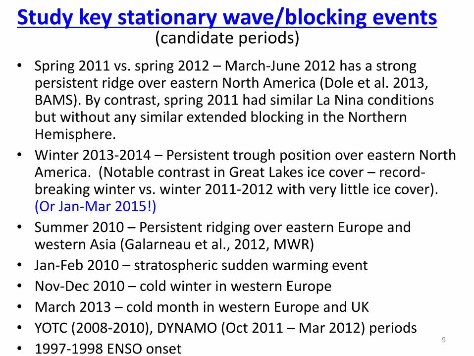
Study key stationary wave/blocking events (candidate periods)
• Spring 2011 vs. spring 2012 – March-June 2012 has a strong persistent ridge over eastern North America (Dole et al. 2013, BAMS). By contrast, spring 2011 had similar La Nina conditions but without any similar extended blocking in the Northern Hemisphere.
• Winter 2013-2014 – Persistent trough position over eastern North America. (Notable contrast in Great Lakes ice cover – record-breaking winter vs. winter 2011-2012 with very little ice cover). (Or Jan-Mar 2015!)
• Summer 2010 – Persistent ridging over eastern Europe and western Asia (Galarneau et al., 2012, MWR)
• Jan-Feb 2010 – stratospheric sudden warming event
• Nov-Dec 2010 – cold winter in western Europe
• March 2013 – cold month in western Europe and UK
• YOTC (2008-2010), DYNAMO (Oct 2011 – Mar 2012) periods
• 1997-1998 ENSO onset
9

FIM numerical atmospheric model •Horizontal grid
• Icosahedral, Δx=240km/120km / 60km/30km/15km/10km
•Vertical grid
• ptop = 0.5 hPa, θtop ~2200K
• Generalized vertical coordinate
• Hybrid θ-σ option (64L, 38L, 21L options currently)
• GFS-like σ-p option (64 levels)
•Physics
• GFS physics suites
• May 2011 version, May 2013 McICA radiation),
• 2015-GFS (incl. “hybrid” EDMF PBL),
• WRF options esp. Grell-Freitas deep/shallow cumulus
•Coupled model extensions
• Chem – WRF-chem/GOCART
• Ocean – icosahedral HYCOM (no coupler),
tri-polar HYCOM (with coupler)
10

Experiments – CMIP – FIM-HYCOM
• Horizontal resolution: 30km.
• Vertical: Atmos: 64 layers.
• Ocean: 26 layers
• Both using vertically adaptive grid
• Physics – atmos: GFS 2015 update physics
• Initial conditions: CFSR atmos & ocean
• Initial time: Dec 11, Jan 12, Feb 12
• Ensemble members 3 for each month
• Forecast duration: 2 months

Evaluation of 2-month forecasts using
Tibaldi-Molteni-defined blocking
NH blocking frequency – DJF 2011-2012
Coupled FIM-HYCOM – 30km

NCEP
Reanalysis
zero month
lead
1 month lead
DEC 2011 JAN 2012 FEB 2012
Coupled FIM-HYCOM
30km
2 month lead
3 month lead
Evaluation
of 3-month
forecasts
using
%-anom
days to
define stat
waves

0 mon lead
1 month lead
Jan 2012 IC x3
2 month lead
Dec 2011 IC
x3
0 month lead
Feb 2012 IC x3
observations
Feb – Mar 2012 TOA outgoing longwave (5oS -15oS average)
Evaluation
of 3-month
forecasts
for OLR for
MJO –
forcing for
stat waves
Coupled FIM-HYCOM
30km

MJO event – OLR
Feb-Mar 2012
Observed
Coupled FIM-iHYCOM
-60km (G7)
Coupled FIM-iHYCOM
-30km (G8)
Improved MJO depiction at 30km
(vs. 60km)

500 AC – ens mean NH-SH
–Jun-Aug2014 - Skill of 10FIM+10GFSens vs.
20GFSens
- Some improvement from mixed-
model ensemble in SH, none in
NH
Improvement from mixed-model ensemble - SH
Improvement from mixed-model ensemble - NH

3rd & 4th Week 2m Temperature Forecast Error in Jan 2012 NCEP 6h reanalysis = truth
Total 8 60km runs, starting at Jan 01 0z, 6z,12z & 18z, with GFS physics and GF, respectively.
30-day FIM AMIP forecasts (GFS-2011 phys)

18
Mean cross-coordinate transport – 24h FIM
quasi-lagrangian hybrid θσ coord (no-physics)
sigma coordinate (no physics)
Stratosphere
Upper
troposphere
Lower
troposphere
1 – stat wave prob 2 – FIM desc 3 – NWP skill 4 – experiments 5 – plans
Reduced cross-coord transport (numerical diffusion) with QL θσ vert coord
Mean abs

θ-σ (solid) vs. σ-p (dashed)
Mean 10hPa zonal wind @60N – Mar2014 – obs vs. FIM fcsts
21 Mar runs capture breakdown, but only θ-σ version for 15 Mar 2-week run
Stratospheric vortex breakdown PV on 600K sfc valid 00 UTC 28 Mar 2014
FIM θ-σ (adaptive) vs. FIM σ-p (fixed) vertical coord

Monthly % of 500 hPa height anomaly days (relative to 30-year mean from Reanalysis)
- θ-σ vs. σ-p FIM 1-yr AMIP runs – Jan 2009
30km 60km 120km 240km Obs
20
θ-σ
σ-p
Feb

21
1-month
– Jan 2012
Obs clouds
GFS with 2014
physics – T574
FIM with GFS-like
sigma vert coord
FIM with θ-σ vert
coord
Better clouds, critical
for coupled
application esp. in
southern oceans.
2014-15 FIM/ESRL activities toward ESPC
- Continued development of FIM-HYCOM
coupled atmos-ocean-chem model
- Physics, dynamics, ocean
- Seasonal and NWP evaluation
2015 - Will start NMME hindcast tests soon
- Rerun blocking/stationary wave exps.
- Bleck et al. (2015-MWR, FIM article)
Atmos-only (AMIP) tests
FIM/HYCOM coupled
atmos/ocean model
•Horizontal grid
• Icosahedral, Δx=30km
•Vertical grid
• Hybrid θ-σ option (64L)
• GFS-like σ-p opt (64L)
•Physics - 2014-GFS, Grell-
Freitas scale-aware cumulus

Stationary Waves Hypotheses on processes for onset/sustenance/cessation Conduct research experiments for 4 stat-wave research ?s (block predictability, Δx/numerics, process pred, physics) Needed experiments for NMME-subseasonal community • Frequency evaluation for blocking and % anom days/mo for extended hindcast for NMME-
subseasonal (and NMME-seasonal) models. • Experiments for YOTC, DYNAMO periods with CFSv2, FIM, (CMIP), blocking processes (MJO,
SSW, etc), physics (CPT)
FIM-HYCOM AMIP/CMIP resolution/coordinate stat-wave-related experiments – FIM – isentropic-sigma vertical coordinate, icosahedral horizontal grid – Resolution –
• More realistic blocking (% anomaly days/month) from higher-res (30, 60km) than coarser-res (120, 240) versions in some seasons (DJF), not in others
• Cold bias (in 500 heights) at coarser resolution (120km, 240km) – Vertical coordinate (θ-σ vs. σ-p )
• Cold bias (in 500 heights) evident with σ-p coordinate, less so with θ-σ • Hypotheses: 1) Cold bias in climate models from vertical diffusion in quasi-
horizontal vertical coordinates (Johnson, 1997, J. Climate , or 2) Difference in precipitation/cloud processes from different vertical coord. • Improved stratospheric sudden warming with θ-σ • Improved MJO with θ-σ, 30km (vs. 60km), CMIP (vs. AMIP)
22