Embed Size (px)
Citation preview

arX
iv:1
504.
0070
6v3
[m
ath.
PR]
21
Aug
201
9
Stationary Distribution Convergence of the Offered Waiting
Processes for GI/GI/1 +GI Queues in Heavy Traffic
Chihoon Lee∗
School of Business
Stevens Institute of Technology
Hoboken, NJ 07030
Amy R. Ward†
Booth School of Business
The University of Chicago
Chicago, IL 60637
Heng-Qing Ye‡
Dept. of Logistics and Maritime Studies
Hong Kong Polytechnic University
Hong Kong
August 23, 2019
Abstract
A result of Ward and Glynn [31] asserts that the sequence of scaled offered waitingtime processes of the GI/GI/1 +GI queue converges weakly to a reflected Ornstein-Uhlenbeck process (ROU) in the positive real line, as the traffic intensity approachesone. As a consequence, the stationary distribution of a ROU process, which is atruncated normal, should approximate the scaled stationary distribution of the offeredwaiting time in a GI/GI/1 + GI queue; however, no such result has been proved.We prove the aforementioned convergence, and the convergence of the moments, inheavy traffic, thus resolving a question left open in [31]. In comparison to Kingman’sclassical result [16] showing that an exponential distribution approximates the scaledstationary offered waiting time distribution in a GI/GI/1 queue in heavy traffic, ourresult confirms that the addition of customer abandonment has a non-trivial effect onthe queue stationary behavior.
Keywords: Customer Abandonment; Heavy Traffic; Stationary Distribution Convergence
∗E-mail: [email protected]†E-mail: [email protected]‡E-mail: [email protected]
1

1 Introduction
There is a long history of studying queueing systems with abandonments, beginning withthe early work of Palm [24] in the late 1930’s. One common objective is to understandthe long time asymptotic behavior of such systems, which is governed by the stationarydistribution (assuming existence and uniqueness). However, except in special cases, themodels of interest are too complex to analyze directly. Instead, some researchers haveexamined the heavy traffic limits of these systems, and developed analytically tractablediffusion approximations (through process-level convergence results). The question oftenleft open is whether or not the stationary distribution of the diffusion does indeed arise asthe heavy traffic limit of the sequence of stationary distributions of the relevant queueingsystem with abandonment. Our objective in this paper is to answer this question for oneof the most fundamental models, the single server queue, operating under the FIFO servicediscipline, with generally distributed patience times; that is, the GI/GI/1 +GI queue.
Our asymptotic analysis relies heavily on past work that has developed heavy trafficapproximations for the GI/GI/1 +GI queue using the offered waiting time process. Theoffered waiting time process, introduced in [2], tracks the amount of time an infinitelypatient customer must wait for service. Its heavy traffic limit when the abandonmentdistribution is left unscaled is a reflected Ornstein-Uhlenbeck process (see Proposition 1,which re-states a result from [31] in the setting in this paper), and its heavy traffic limitwhen the abandonment distribution is scaled through its hazard rate is a reflected nonlineardiffusion (see [27]). However, those results are not enough to conclude that the stationarydistribution of the offered waiting time process converges, which is the key to establishingthe limit behavior of the stationary abandonment probability and mean queue-length.Those limits were conjectured in [27], and shown through simulation to provide goodapproximations. However, the proof of those limits was left as an open question. In thispaper, we focus on the case when the abandonment distribution is left unscaled (i.e., theheavy traffic scaling studied in [31]).
When the system loading factor is less than one, since the GI/GI/1+GI queue is dom-inated by the GI/GI/1 queue, the much earlier results of [16, 17] for the GI/GI/1 queuecan be used to establish the weak convergence of the sequence of stationary distributionsfor the GI/GI/1 +GI queue in heavy traffic. The difficulty arises because, in contrast tothe GI/GI/1 queue, the GI/GI/1 + GI queue can have a stationary distribution whenthe system loading factor equals or exceeds 1 (see [2]). Our main contribution in this pa-per is to establish both the convergence of the sequence of stationary distributions and thesequence of stationary moments of the offered waiting time in heavy traffic, irrespective ofwhether the system loading factor approaches 1 from above or below.
An informed reader would recall [13] and [6], which establish the validity of the heavytraffic stationary approximation for a generalized Jackson network, without customer aban-donment. The proof of the former paper [13] relied on certain exponential integrability
2

assumptions on the primitives of the network and as a result a form of exponential er-godicity was established. The latter paper [6] provided an alternative proof assuming theweaker square integrability conditions that are commonly used in heavy traffic analysis.Our analysis is inspired by the methodology developed in the latter work [6]. However,the main difficulty in extending their methodology to the current model is that the knownregulator mapping under customer abandonment is only locally Lipschitz (that is, the Lips-chitz constant depends on time parameter) whereas the proofs of both [13] and [6] criticallyrely upon the global Lipschitz property of the associated regulator mapping. More pre-cisely, the approaches in [13] and [6] make use of the global Lipschitz continuity propertyof an associated regulator (Skorokhod) mapping to help convert the given moment boundof primitives (the inter-arrival and service times) to the bound of the key performancemeasures (the waiting time or queue-length processes). Such a property is not availablefor the model under study.
In connection to the aforementioned technical issue, the studies of [33, 34] extend theworks of [13] and [6] to a wider range of stochastic processing networks, e.g., the multiclassqueueing network and the resource-sharing network, by relaxing the requirement of theaforementioned Lipschitz continuity. However, their study in [33, 34] deals with networksthat have heavy-traffic limits satisfying the linear dynamic complementarity problem, i.e.,the state process depends on the “free process” (and the regulating process as well) linearly.Therefore, their results do not apply to our GI/GI/1+GI model directly, as the resultingheavy-traffic limit is a reflected Ornstein-Uhlenbeck process and the state process of thislimit (i.e., V (·) in (3) below) depends on the “free process” (i.e., the drifted Brownianmotion in (3)) in a nonlinear manner. Nevertheless, their hydrodynamics approach isadapted to establish a key property, i.e., the uniform moment stability of the offered waitingtime process (see Section 4), in our paper.
A closely related paper is that of Huang and Gurvich [14], which studies the Poissonarrival case (i.e., M/GI/1 +GI queue) and shows the associated Brownian model is accu-rate uniformly over a family of patience distributions and universally in the heavy-trafficregime. For instance, Section EC.3.1 therein corresponds to the critically loaded regime,as considered in this paper. Their approach is based on the generator comparison method-ology, and owing to the Poisson arrivals, it is enough to consider a one-dimensional processwith a simple generator, whereas with general arrival processes, one needs to consider atwo-dimensional process (tracking, e.g., the residual arrival times) and correspondinglymore complicated generator.
In comparison to results for many-server queues, the process-level convergence resultfor the GI/GI/N + GI queue in the quality-and-efficiency-driven regime was establishedin [19] when the hazard rate is not scaled, and in [26], under the assumption of exponentialservice times, when the hazard rate is scaled. Neither paper establishes the convergenceof the stationary distributions. That convergence is shown under the assumption that theabandonment distribution is exponential and the service time distribution is phase type in
3

[10]. The question remains open for the fully general GI/GI/N + GI setting. There hasbeen some progress made in this direction in [15], which establishes the convergence of thesequence of stationary distributions under fluid scaling in the aforementioned fully generalGI/GI/N +GI setting.
The remainder of this paper is organized as follows. We conclude this section with asummary of our mathematical notation. In Section 2, we set up the model assumptions andrecall the known process-level convergence results for the GI/GI/1+GI queue. In Section3, we state our main result, that gives the convergence of the stationary distribution of theoffered waiting time process, and its moments. To prove the main result, we first obtainbounds on the moments of the scaled state process that are uniform in the heavy trafficscaling parameter (n) in Section 4. The proofs of lemmas in this section are technicallyinvolved, and are delayed to Section 6. Lastly, we use uniform moment bounds establishedin Section 4 to prove our main result in Section 5.
Notation and Terminology. Use the symbol “≡” to stand for equality by defi-nition. The set of positive integers is denoted by IN and denote IN0 ≡ IN ∪ 0. LetIR represent the real numbers (−∞,∞) and IR+ the non-negative real line [0,∞). Forx, y ∈ IR, x ∨ y ≡ maxx, y and x ∧ y ≡ minx, y. The function e(·) represents theidentity map; that is, e(t) = t for all t ∈ IR+. For t ∈ IR+ and a real-valued function f ,define ‖f‖t ≡ sup0≤s≤t |f(s)|. Let D(IR) ≡ D(IR+, IR) be the space of right-continuousfunctions f : IR+ → IR with left limits, endowed with the Skorokhod J1-topology (see,for example, [3]). Lastly, the symbol “⇒” stands for the weak convergence; we make thisexplicit for stochastic processes in D(IR), otherwise, it is used for weak convergence for asequence of random variables.
2 The Model and Known Results
The GI/GI/1+GI model having FIFO service is built from three independent i.i.d. se-quences of nonnegative random variables ui, i ≥ 2, vi, i ≥ 1, di, i ≥ 1, that arerepresenting inter-arrival times, service times, and patience times, respectively, and aredefined on a common probability space (Ω,F , IP ). At time 0, the previous arrival to thesystem occurred at time tn0 < 0, so that |tn0 | represents the time elapsed since the lastarrival in the n-th system. We let u1 be the random variable representing the remainingtime conditioned on |tn0 | time units having passed; that is,
IP (u1 > x) = IP (u2 > x|u2 > |tn0 |).
We let F (·) represent the distribution function associated with the patience time d1 and,consistent with [2], assume F (·) is proper. The system primitives are assumed to satisfy:
(A1) For some p ∈ (2,∞), IE[up2 + vp2 ] < ∞, and F ′(0) ∈ (0,∞).
4

We consider a sequence of systems indexed by n ≥ 1 in which the arrival rates becomelarge and service times small. By convention, we use superscript n for any processes orquantities associated with the n-th system. The arrival and service rates in the n-th systemare λn and µn and satisfy the following heavy traffic assumption:
(A2) λn ≡ nλ, limn→∞µn
n = λ ∈ (0,∞) and limn→∞√n(λ− µn
n
)= θ ∈ IR.
The i-th arrival to the n-th system occurs at time
tni ≡i∑
j=1
ujλn
for i ∈ IN,
and has service timevni ≡ vi
µnfor i ∈ IN,
and abandons without receiving service if processing does not begin by time tni + di.
The Offered Waiting Time Process
The offered waiting time process, first given in [2], tracks the amount of time an incom-ing customer at time t has to wait for service. That time depends only upon the servicetimes of the non-abandoning customers already waiting in the queue, that is, those waitingcustomers whose patience time upon arrival exceeds their waiting time. For t ≥ 0, theoffered waiting time process having initial state V n(0) has the evolution equation
V n(t) = V n(0) +
An(t)∑
j=1
vnj 1[V n(tnj −)<dj ] −∫ t
01[V n(s)>0]ds ≥ 0, (1)
whereAn(t) ≡ maxi ∈ IN0 : t
ni ≤ t (2)
is a delayed renewal process when |tn0 | > 0 and is a regular (non-delayed) renewal processwhen tn0 = 0. The quantity V n(t) can also be interpreted as the time needed to emptythe system from time t onwards if there are no arrivals after time t, and hence it is alsoknown as the workload at time t. The initial state V n(0) is 0 if no job is in service andotherwise represents the total workload of all jobs that arrived prior to time 0 and thatwill not abandon before their service begins.
Reflected Ornstein-Uhlenbeck Approximation.
We consider the one-dimensional reflected Ornstein-Uhlenbeck process V ≡ V (t)t≥0
V (t) = V (0) + σW (t) + θλ t− F ′(0)
∫ t0 V (s)ds+ L(t) ≥ 0
subject to: L is non-decreasing, has L(0) = 0 and∫∞0 V (s)dL(s) = 0,
(3)
5

where W (t) : t ≥ 0 denotes a one-dimensional standard Brownian motion, and theinfinitesimal variance parameter is
σ2 ≡ λ−1(var(u2) + var(v2)).
Given F0-measurable initial condition V (0) ≥ 0, the strong existence and pathwise unique-ness of solution (V,L) to the stochastic differential equation (3) hold for the data (V (0),W ),i.e., the solution is adapted to (FW
t ∨ F0)t≥0 (see, e.g., [35]).
The following weak convergence result is a simple modification of Theorem 1(a) of Wardand Glynn [31] and we provide its proof in the Appendix for the sake of completeness.
Proposition 1. Assuming√nV n(0) ⇒ V (0) as n → ∞, we have
√nV n ⇒ V in D(IR) as n → ∞. (4)
3 The Stationary Distribution Existence and ConvergenceResults
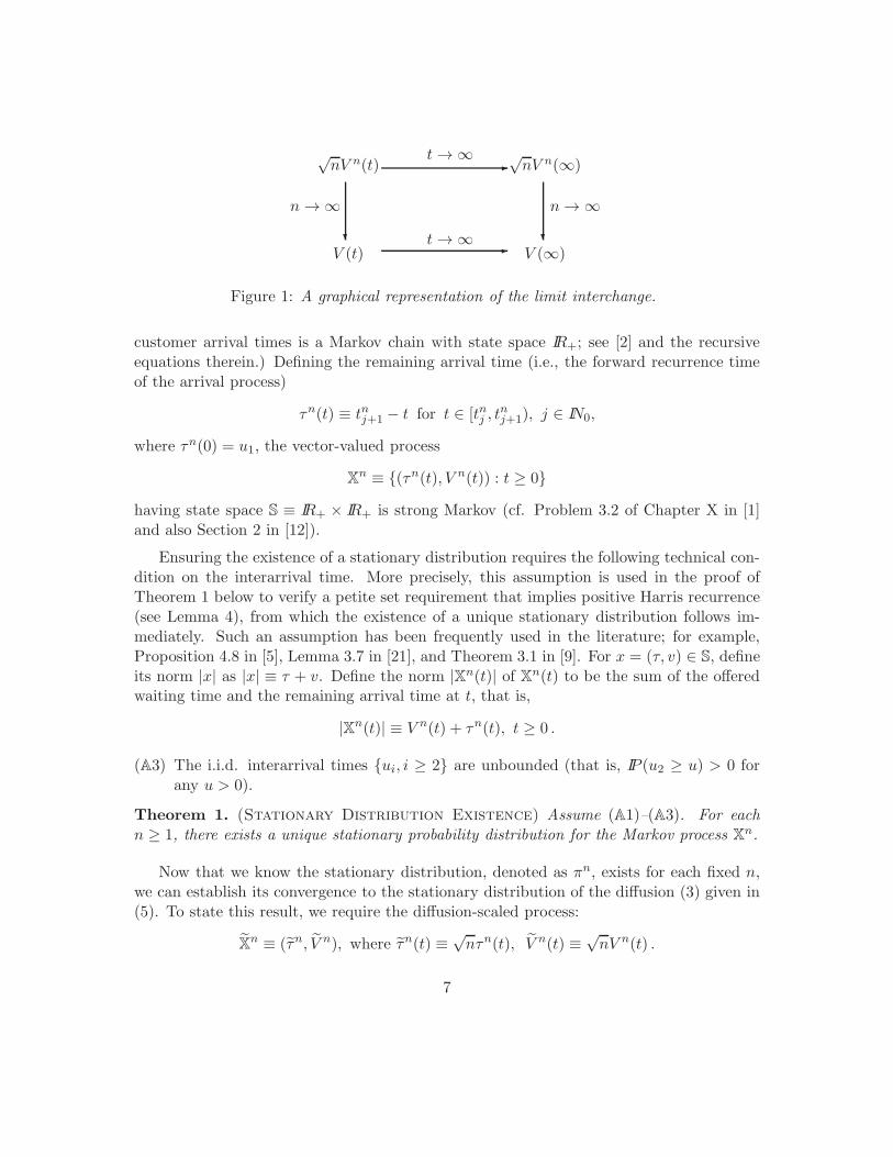
The weak convergence (4) motivates approximating the scaled stationary distributions forV n, and its moments, using the stationary distribution of V , and its moments. Thisrequires establishing the limit interchange depicted graphically in Figure 1. When thelimit n → ∞ is taken first, and the limit t → ∞ is taken second, the convergence is known.More specifically, the convergence as n → ∞ was established in (4), and Proposition 1in [30] shows
V (t) ⇒ V (∞) as t → ∞for V (∞) a random variable having density
f(x) =b−1φ(x−m
b )
1− Φ(−mb )
for x ≥ 0, (5)
where m ≡ θ/(λF ′(0)), b ≡ σ/√
2F ′(0) and φ(·), Φ(·) denote the pdf and cdf of the stan-dard normal distribution, respectively. In other words, V (∞) is distributed as truncatednormal with mean m and variance b2, conditioned to be on IR+.
In this Section, we state our main results, first that a unique stationary distributionexists for each system n, and second that the convergence in Figure 1 is valid when thelimit is first taken as t → ∞ and second taken as n → ∞. In order to do this, we firstspecify the relevant Markov process.
The offered waiting time process V n(t) : t ≥ 0 alone is not Markovian due to theremaining arrival time. (In contrast, the offered waiting time process tracked only at
6
√nV n(t)
√nV n(∞)
V (t) V (∞)
t → ∞
t → ∞
n → ∞ n → ∞
Figure 1: A graphical representation of the limit interchange.
customer arrival times is a Markov chain with state space IR+; see [2] and the recursiveequations therein.) Defining the remaining arrival time (i.e., the forward recurrence timeof the arrival process)
τn(t) ≡ tnj+1 − t for t ∈ [tnj , tnj+1), j ∈ IN0,
where τn(0) = u1, the vector-valued process
Xn ≡ (τn(t), V n(t)) : t ≥ 0
having state space S ≡ IR+ × IR+ is strong Markov (cf. Problem 3.2 of Chapter X in [1]and also Section 2 in [12]).
Ensuring the existence of a stationary distribution requires the following technical con-dition on the interarrival time. More precisely, this assumption is used in the proof ofTheorem 1 below to verify a petite set requirement that implies positive Harris recurrence(see Lemma 4), from which the existence of a unique stationary distribution follows im-mediately. Such an assumption has been frequently used in the literature; for example,Proposition 4.8 in [5], Lemma 3.7 in [21], and Theorem 3.1 in [9]. For x = (τ, v) ∈ S, defineits norm |x| as |x| ≡ τ + v. Define the norm |Xn(t)| of Xn(t) to be the sum of the offeredwaiting time and the remaining arrival time at t, that is,
|Xn(t)| ≡ V n(t) + τn(t), t ≥ 0 .
(A3) The i.i.d. interarrival times ui, i ≥ 2 are unbounded (that is, IP (u2 ≥ u) > 0 forany u > 0).
Theorem 1. (Stationary Distribution Existence) Assume (A1)–(A3). For eachn ≥ 1, there exists a unique stationary probability distribution for the Markov process X
n.
Now that we know the stationary distribution, denoted as πn, exists for each fixed n,we can establish its convergence to the stationary distribution of the diffusion (3) given in(5). To state this result, we require the diffusion-scaled process:
Xn ≡ (τn, V n), where τn(t) ≡ √
nτn(t), V n(t) ≡ √nV n(t) .
7

Notice the time is not scaled in the process V n because the arrival and service rate pa-rameters are scaled instead (from (A2), both λn and µn are order n quantities); therefore,scaling the state by
√n produces the traditional diffusion scaling. Also, a motivation be-
hind the scaling for the residual arrival time τn comes from the way how the√n diffusion
scaling affects the τn under the arrival rate λn = nλ (cf. see (9) below).
Theorem 2. (Stationary Convergence) Assume (A1)–(A3).
(a) (Distribution) Denote by πn0 the marginal distribution of πn on the second coor-
dinate of Xn, i.e., πn0 (A) = πn(IR+ × A) for A ∈ B(IR+). Let V n(∞) be a random
variable having distribution πn0 and also V (∞) a random variable having density (5).
We have that V n(∞) ⇒ V (∞) as n → ∞.
(b) (Moments) For any m ∈ (0, p − 1),
IE[(V n(∞))m] → IE[(V (∞))m] as n → ∞.
Remark 1. (Queue-length Convergence) The queue-length process Qn(t) representsthe number of customers that are in system at time t > 0, either waiting or with theserver. In contrast to V n, Qn includes customers that will eventually abandon but have notyet done so. When the initial condition satisfies Qn(0)/
√n ⇒ Q(0) as n → ∞, Theorem
3 in [31] shows thatQn
√n⇒ λV in D(IR) as n → ∞.
In other words, recalling (4), a process-level version of Little’s law holds. This suggeststhat a version of Theorem 2 should hold for the queue-length process as well. However,proving this is more involved technically due to the need to track both customers in queuethat will eventually receive service and customer in queue that will eventually abandon; seethe “potential queue measure”, a measure-valued state descriptor in Section 2.2 of [15],and also see Figure 4 in [25] for a graphic depiction of that measure. This is the reasonwe leave that analysis as future research.
4 Uniform Moment Estimates
The proofs of both Theorems 1 and 2 rely on a tightness result for the family of stationarydistributions of Xnn≥1. The key to the desired tightness is to obtain uniform (in n)bounds for the moments of the stationary distributions. Henceforth, we use the subscript xto denote the scaled Markov process Xn has an initial state (τn(0), V n(0)) = (τ, v) ≡ x ∈ S.Our convention is to subscript any process that depends on the initial state x ∈ S by x.Then, V n
x has initial state V n(0) = v/√n and is defined from the process V n
x in (1) thatuses the (delayed) renewal process An
x in (2). Recall the norm |x| of x = (τ, v) ∈ S isdefined as |x| ≡ τ + v.
8

Proposition 2. Assume (A1)–(A2). Let q ∈ [1, p). There exists t0 ∈ (0,∞) such that forall t ≥ t0,
lim|x|→∞
supn
1
|x|q IE[|Xn
x(t|x|)|q]= 0. (6)
Before proving Proposition 2, we provide a roadmap about how it will be used inthe proofs of the main results. Proposition 2 yields uniform (in the scaling parameter)moment bounds for the scaled Markov process of the GI/GI/1 +GI system. We use suchuniform moment estimates, in conjunction with the Lyapunov function methods of Meynand Tweedie [23] and Dai and Meyn [11], in order to obtain time uniform moment bounds(via weighted return time estimates) for the aforementioned scaled Markov process. Then,the sought-after moment bounds for the stationary distributions, uniform in the scalingparameter, readily follow (see (26) and (28) in the proof of Theorem 2) and this yieldstightness of the collection of the stationary distributions and hence Theorem 2.
The crux in proving Proposition 2 lies in two versions of pathwise stability results(Lemmas 1 and 2), whose intuitive ideas are provided right after stating those results. Theproof of Proposition 2 relies on a martingale representation of the offered waiting timeprocess. We first provide this setup, and second give the proof.
4.1 Martingale Representation and Diffusion Scaling
Define the σ-fields (Fni )i≥1 where
Fni ≡ σ((tn1 , v
n1 , d1), . . . , (t
ni , v
ni , di), t
ni+1) ⊆ F ,
and let Fn0 ≡ σ(tn1 ). Notice that V n
x (tni −) is Fni−1-measurable and the patience time di of
the i-th customer is independent of Fni−1. Hence,
IP [V nx (tni −) ≥ di|Fn
i−1] = F (V nx (tni −)), i = 1, 2, . . . , (7)
holds almost surely, recalling that F is the distribution function of di. We then have amartingale with respect to the filtration (Fn
i )i≥1 given by
Mnx (i) ≡
i∑
j=1
(1[V n
x (tnj −)≥dj ] − IE(1[V nx (tnj −)≥dj ]|Fn
j−1)).
Using (7), we also see that for all i ∈ IN
Mnx (i) =
i∑
j=1
[1[V n
x (tnj −)≥dj ] − F (V nx (tnj−))
].
9

Next, define the following centered quantities
Sn(i) ≡ 1
n
i∑
j=1
(vj − 1), Snd,x(i) ≡
1
n
i∑
j=1
(vj − 1)1V nx (tnj −)≥dj.
From (1), algebra, and the above definitions, we have for t ≥ 0
V nx (t) =
v√n− t− 1
µn
An(t)∑
j=1
F(V nx (tnj−)
)+
∫ t
01V n
x (s)=0ds (8)
+n
µn
(An
x(t)
n+ Sn (An
x(t))− Snd,x(A
nx(t))−
1
nMn
x (Anx(t))
).
With the initial state Xn(0) = (τ, v) ≡ x ∈ S, define fluid-scaled and diffusion-scaled
quantities to carry out our analysis. For t ≥ 0, let
Anx(t) ≡
Anx(t)
n, An
x(t) ≡√n
(1
nAn
x(t)− λ(t− τ√n∧ t)
), Sn(t) ≡ √
nSn([nt]), (9)
Snd,x(t) ≡
√nSn
d ([nt]) , Mnx (t) ≡
1√nMn
x ([nt]).
Algebra, (8) and substitution of the above scaled quantities into the scaled offered waitingtime process
V nx (·) ≡ √
nV nx (·),
shows that for t ≥ 0
V nx (t) = v + bnt+ Nn
x (t)−n
µn
∫ t
0
√nF
(1√nV nx (s−)
)dAn
x(s) + Inx (t), (10)
where
bn ≡(
n
µn
)√n
(λn
n− µn
n
)
Nnx (t) ≡
(n
µn
)(Sn(An
x(t))− Snd,x(A
nx(t))− Mn
x (Anx(t)) + An
x(t)),
Inx (t) ≡ √n
∫ t
01[V n
x (s)=0]ds .
10

4.2 Proof of Proposition 2
We will establish the claim when q ∈ [2, p). Then the claim with q ∈ [1, 2) follows fromJensen’s inequality. From the inequality (cf. Lemma 2 on page 98 in [28])
(a+ b)r ≤ (1 ∨ 2r−1)(ar + br) for a, b, r ≥ 0,
we obtain for q ∈ [2, p) that
IE[∣∣∣Xn
x(t|x|)∣∣∣q]
≤ 2q−1(IE [τnx (t|x|)q] + IE
[V nx (t|x|)q
]).
Therefore, it is sufficient to show that there exists t0 ∈ IR+ such that for all t ≥ t0,
lim|x|→∞
supn
1
|x|q IE [τnx (t|x|)q] = 0 (11)
and
lim|x|→∞
supn
1
|x|q IE[V nx (t|x|)q
]= 0 (12)
We first show (11) and second show (12).
Proof of (11). We begin by observing that by definition τnx (t|x|) ≤√nu(An
x (t|x|)+1)/(λn),for all t ≥ 0 and x ∈ S. Next, define the regular (non-delayed) renewal process An
2 (·) via
An2 (t) ≡ max
i ∈ IN :
i∑
j=1
uj+1
λn≤ t
, t ≥ 0,
where the maximum over an empty set is 0, and observe that
Anx(t) ≤ An
2 (t) + 1.
Now, take t0 = 1. Then, for t ≥ t0,
τnx (t|x|)q ≤ nq/2
Anx (t|x|)+1∑
k=2
( ukλn
)q≤ nq/2
An2(t|x|)+2∑
k=2
( ukλn
)q,
where the first inequality above uses the fact that Anx(t|x|) ≥ 1 because t0|x| = |x| ≥ τ ≥
u1 = τ/√n. From Wald’s identity,
IE
An
2(t|x|)+2∑
k=2
( ukλn
)q
= IE [An
2 (t|x|) + 1]IE[uq2]
λqnq.
11

Together, the above two displays imply
IE [τnx (t|x|)q] ≤1
λq
1
nq/2IE[uq2]IE [An
2 (t|x|) + 1] . (13)
From the elementary renewal theorem, for any t > 0 and fixed n,
IE [An2 (t|x|)]
λnt|x| → 1 as |x| → ∞,
and soIE [An
2 (t|x|)] ≤ 1 + λnt|x|, for all large enough |x|. (14)
Substituting (14) into the right-hand-side of (13) shows that for any t ≥ t0 and fixed n
IE [τnx (t|x|)q] ≤1
λq
1
nq/2IE[uq2](2 + λnt|x|) ≤ 1
λq
1
nq/22IE[uq2] (1 + λnt|x|) , (15)
where the second inequality follows provided λnt|x| ≥ 1, which is true for large enough |x|and fixed n. Finally, (11) follows from (15) taking, for example, t0 = 1.
To complete the proof, we must show (12), which is more involved than (11), andproceeds following the approach of Ye and Yao ([33], Lemma 10 and Proposition 11).First, we establish two versions of pathwise stability results (Lemmas 1 and 2), one for any(fixed) n-th system and the other for the whole sequence. With the moment condition (A1)on the system primitives, the pathwise stability results are then turned into the momentstability in Lemma 3, which finally leads to (12).
Lemma 1. (Stability of V n(·) for any (fixed) n) Let rii≥1 be a sequence of num-bers such that ri → ∞ as i → ∞ and assume the sequence of initial states xi ∈ Si≥1
satisfies |xi| ≤ ri for all i. Pick any constant c > 1. Then, for any fixed n, the followingholds (with probability one),
limi→∞
1
riV nxi(rit) = 0, u.o.c. for t ≥ c√
n. (16)
Lemma 2. (Stability of V n(·)) Let rn be a sequence of numbers such that rn → ∞as n → ∞ and assume that the sequence of initial states xn ∈ Sn≥1 satisfies |xn| ≤ rn.Then, for any ǫ > 0, the following holds (with probability one),
limn→∞
1
rnV nxn(rnt) = 0, u.o.c. for t ≥ ǫ. (17)
Lemma 3. (Moment stability) Assume (A1) and (A2).(a) Letting ri and xi as in Lemma 1,
limi→∞
IE1
rqiV nxi(rit)
q = 0, for t ≥ 1√n. (18)
12

(b) Letting rn and xn as in Lemma 2,
limn→∞
IE1
rqnV nxn(rnt)
q = 0, for t > 0. (19)
While the proofs of the above three lemmas are provided in Section 6, we provide someintuitions here, for Lemmas 1 and 2 in particular. Consider the (fixed) n-th system inLemma 1. During the initial period, if it starts with a large initial state, say, V n
xi(0) = ri,new arrivals will abandon the service with nearly probability one. On the other hand,the existing workload, under fluid scaling as in (16), drains (i.e., is processed) at the rate√n approximately. Therefore, the workload V n
xi(t) will reach the “normal” operating stateafter the initial period with an order of ri/
√n. The normal operating state, scaled by 1/ri
(where ri → ∞), will be approximately zero, and this is characterized by the convergencein (16). In Lemma 2, the index n approaches infinity. For large n and hence large rn,consider the n-th (scaled) system and suppose it restarts at a time t, i.e., 1
rnV nxn(rn(t+ ·)).
Then, the key observation is similar to the above case; that is, if the initial state (startingat t) is bounded by a constant (say, 1
rnV nxn(rnt) ≤ 1), it should be approximately zero after
a time of O(1/√n). Indeed by applying Bramson’s hydrodynamic approach, we are able to
bound 1rnV nxn(rnt) for any time t during the (arbitrarily given) period [0, T ]. Therefore, our
key observation applies for any time t, which will establish (17). Lastly, Lemma 3 plays apivotal role in establishing the key moment estimate in (12). Given Lemma 3, the proof of(12) repeats the one for Proposition 11 of [33] and is provided below for completeness.
Proof of (12). Pick any time t > 0. Suppose (12) does not hold; then, there exists anǫ0 > 0 and a sequence of initial states xi ∈ S : i = 1, 2, . . . satisfying limi→∞ |xi| = ∞such that
supn
1
|xi|q IE∣∣∣V n
xi(t|xi|)∣∣∣q> 2ǫ0. (20)
Corresponding to each xi, choose an index in the sequence nn≥1, denoted by ni, suchthat
1
|xi|q IE∣∣∣V ni
xi (t|xi|)∣∣∣q> ǫ0. (21)
We claim that nii≥1 cannot be bounded. Otherwise, at least an index, say n′, repeats inthe sequence for infinitely many times; this contradicts to Lemma 3(a). Otherwise, withoutloss of generality, assume ni → ∞ as i → ∞. Then, the bound in (21) contradicts to Lemma3(b). We conclude that the aforementioned sequence of initial states xi ∈ S : i = 1, 2, . . .satisfying (20) cannot exist, which implies (12) holds.
13

5 Proofs of the Main Results (Theorems 1 and 2)
Proof of Theorem 1. From Proposition 2, there exists δ ≡ t0 > 0 such that
lim|x|→∞
1
|x|IE|Xnx(|x|δ)| = 0. (22)
We require the following lemma, whose proof follows along the same lines of Proposition4.8 in Bramson [5]. We provide its proof and the notion of petite set in the Appendix forthe sake of completeness.
Lemma 4. Assume (A3). The set C = x ∈ S : |x| ≤ κ is closed petite for every κ > 0.
Given Lemma 4, Theorem 3.1 of [9] implies the Markov process Xn(·) and the scaled
process Xn(·) are positive Harris recurrent and hence the existence of a unique stationarydistribution follows.
Having Proposition 2 and Theorem 1 at hand, the proof of Theorem 2 follows a simi-lar outline to that of Theorem 3.1 in [6]. (Recall [6] establishes the validity of the heavytraffic stationary approximation for a generalized Jackson network without customer aban-donment, assuming the inter-arrival and service time distributions have finite polynomialmoments, as in (A1).) A global strategy of the proof is as follows. First, Proposition 3 be-low establishes uniform (in n) estimates on the expected return time of the general Markovprocess to a compact set. Second, from such return time estimates, moment bounds for thestationary distributions of Xn, uniform in the scaling parameter n, follow readily, yield-ing tightness of these distributions. Third, the distributional convergence in Theorem 2(a)follows by combining this tightness property with the known weak convergence results ofV n in (4) and [31]. Next, we obtain convergence of moments of stationary distributions,i.e., Theorem 2(b). We begin by providing a general statement concerning strong Markovprocesses.
Proposition 3. (Theorem 3.5 of [6], cf. Proposition 5.4 of [11]) For n ≥ 1, consider astrong Markov process Yn
x(t) : t ≥ 0 with initial condition x on a state space T. For δ ∈(0,∞), define the return time to a compact set C ⊂ T by τnC(δ) ≡ inft ≥ δ : Yn
x(t) ∈ C.Let f : T → [0,∞) be a measurable map. For δ ∈ (0,∞) and a compact set C ⊂ T, define
Gn(x) ≡ IE
[∫ τnC(δ)
0f(Yn
x(t))dt
], x ∈ T.
If supnGn is everywhere finite and uniformly bounded on C, then there exists a constantη ∈ (0,∞), that is independent of n, such that for all n ∈ IN , t ∈ (0,∞), x ∈ T,
1
tIE[Gn(Y
nx(t))] +
1
t
∫ t
0IE[f(Yn
x(s))]ds ≤ 1
tGn(x) + η. (23)
14

Proof of Theorem 2. We first prove (a) and then (b).
Part (a): Using standard arguments (cf. [13]), it suffices to establish the tightness ofthe family of stationary distributions πn : n ≥ 1. Indeed, the tightness implies everysubsequence of πn : n ≥ 1 admits a convergent subsequence. Denote a typical limit pointby π and also define the marginal distribution (corresponding to the limiting stationarydistribution of V n) π0 as π0(A) ≡ π(IR+ × A), A ∈ B(IR+). Then, as in (4), we see thatthe process V n, with X
n(0) distributed as πn, converges in distribution to V defined in (3)with V (0) ∼ π0. The stationarity of V n implies that π0 is a stationary distribution for V .Since V has a unique stationary distribution, say π, it must be π0 = π.
To prove the desired tightness, it suffices to show that there exists a positive integer Nsuch that for all n ≥ N ∫
S
|y|πn(dy) ≤ c, (24)
where c ∈ (0,∞) is a constant independent of n. The following arguments proceed accord-ing to the same outline as the proof of Theorem 3.2 of [6], but with some details that differ.A key observation from Proposition 2 is that there exists γ0 ∈ (0,∞) such that, for t0 asin that same proposition,
supn
IE|Xnx(t0|x|)|q ≤
1
2|x|q, for all x ∈ Cc, C ≡ x ∈ S : |x| ≤ γ0. (25)
Next, we apply Proposition 3 above with
Ynx = X
nx, T = S, δ ≡ t0γ0, f(x) ≡ 1+ |x|q−1 for x ∈ S, q ∈ [2, p), C ≡ x ∈ S : |x| ≤ γ0.
Suppose we can show that there exist N ∈ IN and c ∈ (0,∞) such that
supn≥N
Gn(x) = supn≥N
IE
[∫ τnC(δ)
0(1 + |Xn
x(t)|q−1)dt
]≤ c(1 + |x|q), x ∈ S, (26)
so that the conditions of Proposition 3 are satisfied for the family Xnx : n ≥ N. Then,
for x ∈ S and η ∈ (0,∞) as in Proposition 3,
Φn(x) ≡1
tGn(x)−
1
tIE[Gn(X
nx(t))] ≥
1
t
∫ t
0IE(f(Xn
x(s)))ds − η,
15

and thus an expectation with respect to the stationary distribution πn has a lower bound,
∫
S
Φn(x)πn(dx) ≥
∫
S
(1
t
∫ t
0IE(f(Xn
x(s)))ds − η
)πn(dx)
=
∫
S
(1
t
∫ t
0IE(f(Xn
x(s)))ds
)πn(dx) − η
=1
t
∫ t
0
(∫
S
IE(f(Xnx(s)))π
n(dx)
)ds− η (27)
=
∫
S
f(x)πn(dx)− η, (28)
where (27) is from Fubini’s theorem and (28) follows from the fact that πn is a stationarydistribution. Furthermore, if Φn(x) is a bounded function in x, then from the definitions ofthe stationary distribution πn and the function Φn(x), it is seen that 0 =
∫SΦn(x)π
n(dx).Otherwise, if Φn(x) is unbounded, then Fatou’s lemma implies that (cf. proof of Theorem3.2 in [6] on page 55, also proof of Theorem 5 in [13])
0 ≥∫
S
Φn(x)πn(dx). (29)
Finally, it follows from (28)–(29) that
0 ≥∫
S
Φn(x)πn(dx) ≥
∫
S
f(x)πn(dx)− η, (30)
which establishes the desired uniform moment bound in (24).
To complete the proof of part (a), it only remains to show (26). The following argumentsare similar to those leading to Theorem 3.4 in [6]. We note that the terms δ, f(x), andthe compact set C are chosen exactly the same way as in the cited theorem. However,minor modifications are necessary because the Markov process Xn
x in this paper is defineddifferently from the Markov process Xn
x in [6]. This entails to checking the following bound,which corresponds to (38) in [6]: there exist N ∈ IN and c0 ∈ (0,∞) such that
supn≥N
IE
[∫ σ1
0
(1 + X
nx(t)
)q−1dt
]≤ c0 (1 + |x|q) , x ∈ S, (31)
where σ1 ≡ t0 (|x| ∨ γ0) is defined exactly as in the proof of Theorem 3.4 in [6]. Noticethat σ1 ≤ c1(1+ |x|) for some c1 ∈ (0,∞), which is the same estimate as in (39) of [6]. Fort ≥ 0 and a real-valued function f on IR+, define ‖f‖t ≡ sup0≤s≤t |f(s)|. To show (31),it is sufficient to show there exist constants c2, c3 ∈ (0,∞), and N ∈ IN such that, for alln ≥ N ,
IE∥∥∥V n
x
∥∥∥q−1
c1(1+|x|)≤ c2 (1 + |x|)q−1 (32)
16

andIE ‖τnx ‖q−1
c1(1+|x|) ≤ c3(1 + |x|)q−1. (33)
The argument to show (32). It follows from the proof of Lemma 3 (more precisely, (61) in
Section 6 and the fact that ||V nx ||t ≤ ||W n
x ||t, where W nx (t) : t ≥ 0 denotes the offered
waiting time process of the GI/GI/1 queue defined as in the proof of Lemma 3).
The argument to show (33). The same logic used to show (13) also shows
IE [τnx (t)q] ≤ 1
λq
1
nq/2IE [uq2] (IE [An
2 (t)] + 1) , for t ≥ 0,
where An2 is the regular (non-delayed) renewal process defined in the second paragraph of
the proof of Proposition 2. Since An2 is a non-decreasing process,
IE [τnx (t)q] ≤ 1
λq
1
nq/2IE[uq2] (IE [An
2 (c1 + (1 + c1)|x|)] + 1) , for 0 ≤ t ≤ c1(1 + |x|).
From the elementary renewal theorem, there exists N ∈ IN such that for all n ≥ N ,
IE [An2 (c1 + (1 + c1)|x|)] ≤ λn (c1 + (1 + c1)|x|+ 1) = λn(1 + c1)(1 + |x|),
and so
IE [τnx (t)q] ≤ 1
λqn1−q/2IE[uq2] (λ(1 + c1)(1 + |x|) + 1) , for n ≥ N and 0 ≤ t ≤ c1(1 + |x|).
Recalling that q ≥ 2 and n ≥ 1 ensures n1−q/2 ≤ 1 and so
IE [τnx (t)q] ≤ 1
λqIE[uq2] (λ(1 + c1) + 1) (1 + |x|), for n ≥ N and 0 ≤ t ≤ c1(1 + |x|).
Since 0 < q − 1 < q, Holder’s inequality implies
IE[τnx (t)
q−1]≤ (IE [τnx (t)
q])(q−1)/q , for t ≥ 0.
Hence for c3 ≡ (IE[uq2] (λ(1 + c1) + 1) /λq)(q−1)/q
,
IE[τnx (t)
q−1]≤ c3 (1 + |x|)(q−1)/q ≤ c3(1 + |x|)q−1, for n ≥ N and 0 ≤ t ≤ c1(1 + |x|),
from which (33) follows.
Part (b): Proposition 2 implies the moment estimate (25) with q ∈ [1, p). However, whenapplying Proposition 3 with f(x) ≡ 1+ |x|q−1, we require q ∈ [2, p) in order to obtain (33)and (30). Therefore, we have a uniform (in n) moment bound on the (q− 1)-th moment ofthe family of stationary distributions πnn≥1. If we pick q such thatm < q−1, this uniform
moment bound, in turn, implies the uniform integrability of |Xn|mn≥1 with m ∈ (0, q−1)
in stationarity (i.e., Xn(0) ∼ πn). Combining the weak convergence result established inpart (a) and the aforementioned uniform integrability, we conclude the desired momentconvergence in stationarity as in part (b). This completes the proof.
17

6 Proofs of Lemmas 1–3
Proof of Lemma 1. Without loss of generality, assume that as i → ∞, xi/ri → x ≡(τ , v(0)) with |x| = τ + v(0) ≤ 1; otherwise, it suffices to consider any convergent subse-quence. Fix the index n throughout the proof. We also omit the index n and the subscriptxi whenever it does not cause any confusion.
For the i-th copy of the n-th system, write the offered waiting time as:
1
riV nxi(rit) ≡ vi(t) = φi(t) + ηi(t), with (34)
φi(t) ≡ vi
ri+
n√n
µn· 1
rin
An(rit)∑
j=1
(1− F (V n(tnj−)))−√nt
+n√n
µn· 1ri
(Sn(An(rit))− Sn
d (An(rit))−
1
nMn(An(rit))
), (35)
ηi(t) ≡√n
ri
∫ rit
01V n(s)=0ds. (36)
First, estimate the item associated with the arrival in the above (in the first summation):
An(rit)
rin=
1
rin
(An(rit)− λn(rit−
τi√n∧ rit)
)+ λ(t− τi
ri√n∧ t)
→ λ(t− τ√n∧ t), as i → ∞ a.s. (37)
Second, denote the term associated with the arrival and abandonment as
ξi(t) ≡1
rin
An(rit)∑
j=1
(1− F (V n(tnj−))). (38)
Observe that for any 0 ≤ t1 < t2, we have
0 ≤ ξi(t2)− ξi(t1) ≤1
rin(An(rit2)−An(rit1)). (39)
From (37), we note that the right-hand side in the above converges uniformly to λ(t2 −t1 − τ√
n∧ t2 +
τ√n∧ t1). Therefore, any subsequence of i contains a further subsequence
such that as i → ∞ along the further subsequence, we have the weak convergence
ξi(·) ⇒ ξ(·), in D(IR) as i → ∞,
18

where the limit ξ(·) is Lipschitz continuous (recall (39)) with a Lipschitz constant λ (withprobability one). Without loss of generality, we can assume the above convergence is alongthe full sequence, and furthermore, by using the coupling technique, we can further assumethe convergence is almost surely:
ξi(t) → ξ(t), as i → ∞ a.s.
Third, for the martingale terms, we have as i → ∞ with probability one,
1
ri
(Sn(An(rit))− Sn
d (An(rit))−
1
nMn(An(rit)
)→ 0. (40)
Putting the above convergences together yields, as i → ∞,
φi(t) → φ(t) ≡ v(0) +n√n
µnξ(t)−√
nt, u.o.c. of t ≥ 0. (41)
Note from (34)–(36) that the tuple (vi(t), φi(t), ηi(t))t≥0 satisfies the one-dimensional linearSkorokhod problem (cf. §6.2 of [7]):
vi(t) = φi(t) + ηi(t) ≥ 0, dηi(t) ≥ 0 with ηi(0) = 0, vi(t)dηi(t) = 0.
Hence, by invoking the Lipschitz continuity of the Skorokhod mapping (cf. Theorem 6.1of [7]), the convergence in (41) implies
1
riV nxi(rit) → v(t) and ηi(t) → η(t) u.o.c. of t ≥ 0, (42)
with the limit satisfying the Skorokhod problem as well:
v(t) = φ(t) + η(t) ≥ 0, dη(t) ≥ 0 with η(0) = 0, v(t)dη(t) = 0. (43)
Next, we further examine the limit ξ(·) following the approach of Chen and Ye ([8],
Proposition 3(b)). From (37) and (38), and noting that ξi(t) ≤ An(rit)rin
, we have
ξ(t) = 0, 0 ≤ t ≤ τ√n. (44)
Now, consider any regular time t1 > τ/√n, at which all processes concerned, i.e., v(·), φ(·),
and η(·) are differentiable, and v(t1) > 0. Note that the Lipschitz continuity of ξi(·) impliesthat (v(·), φ(·), η(·)) are also Lipschitz continuous. Therefore, we can find (small) constantsǫ > 0 and δ > 0 such that the following inequality holds for all sufficiently large i:
vi(t2) > ǫ i.e., V n(rit2) > riǫ, t2 ∈ [t1, t1 + δ). (45)
19

Observe that if the j-th arrival falls between An(rit1)+1 and An(rit2), then its arrival time,tnj , shall also falls between the corresponding time epochs, i.e., rit1 < tnj ≤ rit2. Given theestimate in (45), this implies the following estimate holds:
V n(tnj ) > riǫ.
Consequently, we have for all sufficiently large i that
ξi(t2)− ξi(t1) =1
rin
An(rit2)∑
j=An(rit1)+1
(1− F (V n(tnj−)))
≤ 1
rin(An(rit2)−An(rit1))(1 − F (riǫ)), t2 ∈ [t1, t1 + δ).
Taking i → ∞, the above yields ξ(t2)− ξ(t1) ≤ 0, which is effectively ξ(t2)− ξ(t1) = 0. Insummary, the above implies for any regular time t > τ/
√n with v(t) > 0,
dξ(t)
dt= 0. (46)
Finally, using the properties in (41), (43), (44) and (46), it is direct to show thatv(t) = v(0)−√
nt for t ≤ v(0)/√n(≤ 1/
√n) and v(t) = 0 for t ≥ v(0)/
√n. This property,
along with the convergence in (42) yields the desired convergence in (16).
Proof of Lemma 2. We adopt Bramson’s hydrodynamics approach (cf. [4, 20, 32]), andits variation (in Appendix B.2 of [33]) in particular, to examine the processes involved in(17). Define for each n and for j = 0, 1, . . .,
V n,j(u) =1
rnV nxn(rn
j + u√n
), u ≥ 0. (47)
That is, the n-th diffusion-scaled process (say, 1rnV nxn(rnt)t≥0) breaks into many pieces of
fluid-scaled process (i.e., V n,j(u) : u ∈ [0, 1] and j = 0, 1, . . .), with each piece covering aperiod of 1/
√n in the diffusion-scaled process. (As in the proof of the previous Lemma 1,
we omit the index n and the subscript xn whenever it does not cause any confusion.)
Let jn be any nonnegative integer for each n and consider any subsequence of positiveinteger, denoted N . If lim supn→∞,n∈N [V n,jn(0)] ≤ 1, then it can be seen that: as n → ∞along N ,
V n,jn(u) → 0, u.o.c. of u ≥ 1. (48)
This can be proved in the same manner as Lemma 1, with extra modification on the shiftedinitial residual arrival time and the sequence of scaling factors (rn/
√n here versus ri
20

of Lemma 1). We defer the proof of (48) for now, and proceed to show the main claim in(17).
To prove (17), given the hydrodynamic representation of the waiting time in (47), itsuffices to show that for any ∆ > 0 and ǫ > 0, the following holds for sufficiently large nand for j = 1, . . . , ⌊√n∆⌋ (excluding j = 0),
V n,j(u) ≤ ǫ, for u ∈ [0, 1]. (49)
We prove this by contradiction. Suppose to the contrary, there exists a subsequence N ,and for all n ∈ N , we can find an integer index jn ∈ [1,
√n∆] and a time un ∈ [0, 1] such
that
V n,jn(un) > ǫ. (50)
Furthermore, we can require that for each n ∈ N , jn is the smallest integer (in [1,√n∆])
for the above inequality to hold.
Observe that the following initial condition must hold for sufficiently large n ∈ N :
V n,jn−1(0) ≤ 1. (51)
First, if jn = 1, then from the definition in (47), we evaluate the left-hand side of the aboveas:
V n,0(0) =1
rnV nxn(0) ≤ |xn|
rn≤ 1.
On the other hand, we have jn ≥ 2; and according to the definition of jn, it means thatthe inequality (49) applies for j = jn − 1. As a result, the inequality (51) also holds.
Given the above initial condition, applying (48) yields the following convergence asn → ∞ in N ,
V n,jn−1(u) → 0, u.o.c. of u ≥ 1.
Therefore, for sufficiently large n ∈ N , we have
V n,jn(u) = V n,jn−1(1 + u) ≤ ǫ, u ∈ [0, 1],
which contradicts to (50), and this establishes the desired result in (17).
Finally, it remains to show the claim (48) holds, which resembles the proof of Lemma 1and hence we provide the outline only. Without loss of generality, assume that as n → ∞,V n,jn(0) → v(0) ≤ 1. Similar to (34), the offered waiting time for the n-system can beexpressed as
V n,jn(u) =1
rnV n(rn
jn + u√n
) ≡ vn(u) ≡ φn(u) + ηn(u), (52)
21

where
φn(u) ≡ V n,jn(0) +n
µn· 1
rn√n
An(rn(jn+u)/√n)∑
j=An(rnjn/√n)+1
(1− F (V n(tnj−)))− u
+n
µn·√n
rn
(Sn(An(rn
jn + u√n
))− Sn(An(rnjn√n))
)
− n
µn·√n
rn
(Snd (A
n(rnjn + u√
n))− Sn
d (An(rn
jn√n))
)
− n
µn· 1
rn√n
(Mn(An(rn
jn + u√n
)−Mn(An(rnjn√n)
),
ηn(u) ≡√n
rn
∫ jn+u√n
jn√n
1V n(s)=0ds.
In parallel to the convergence in (37), we have:
1
rn√n
(An(rn
jn + u√n
)−An(rnjn√n)
)
=1
rn√n
(An(rn
jn + u√n
)−An(rnjn√n)− λrn
√n
(u− u ∧
(1
rnτn(rn
jn√n)
)))
+λ
(u− u ∧
(1
rnτn(rn
jn√n)
))
→ λu, as n → ∞ a.s. (53)
While the convergence in (37) is justified by the conventional functional strong law of largenumbers for a renewal process (e.g., [7]), we have applied here a version established byBramson ([4], Proposition 4.2) and Stolyar ([29], Appendix A.2), which accompanies thehydrodynamic scaling approach.
Then, following the arguments from (38)–(43), it is seen that, as n → ∞,
(V n,jn(u), φn(u), ηn(u)) → (v(u), φ(u), η(u)) u.o.c. of u ≥ 0, (54)
where
φ(u) = v(0) +1
λξ(u)− u. (55)
Moreover, the limits, ξ(·), v(·), φ(·) and η(·), are Lipschitz continuous and satisfy theSkorokhod problem:
v(u) = φ(u) + η(u) ≥ 0, dη(u) ≥ 0 with η(0) = 0, v(u)dη(u) = 0. (56)
22

Next, a similar analysis on the limit ξ(·) yields that, for any regular time u > τ withv(u) > 0,
dξ(u)
du= 0. (57)
Finally, using the properties in (55), (56) and (57), it is direct to show that v(u) =v(0) − u for u ≤ v(0)(≤ 1) and v(u) = 0 for u ≥ v(0). This property, along with theconvergence in (54) yields the desired convergence in the claim (48).
Proof of Lemma 3. We first show that for any (fixed) p′ ∈ (q, p), there exists a constantκ′ ∈ (0,∞) such that the following bound holds for any initial state x and any time t ≥ 0,
IE[V nx (t)]p
′ ≤ κ′(1 + |x|p′ + tp′). (58)
Indeed, if we discard the abandonment component, the systems will be reduced to themore basic GI/GI/1 queues. Dropping the abandonment component in the original stateequation (1), one gets the offered waiting time process W n(t) : t ≥ 0, for the n-th system,as
W nx (t) = V n
x (0) +
Anx(t)∑
j=1
vnj −∫ t
01[Wn
x (s)>0]ds.
Then, because the system without abandonment dominates the system with abandonmentat all times (as can be seen using the one-dimensional Skorokhod mapping), V n
x (t) ≤ W nx (t)
for all t ≥ 0. Rewrite the above, with diffusion scaling, as,
W nx (t)[≡
√nW n
x (t)] = V nx (0) + ξn(t) +
√n
∫ t
01[Wn
x (s)=0]ds,
where
ξn(t) ≡ √n
Anx (t)∑
j=1
vnj −√nt
=
√n
µn
Anx(t)∑
j=1
(vj − 1) +
√n
µn(An
x(t)− nλt) +√n
(λ− µn
n
)n
µnt.
=n
µn(Sn(An
x(t)) + Anx(t) + θnt). (59)
Observe that W nx (·) = Φ(V n
x (0) + ξn(·)), where Φ is the standard one-dimensional Sko-rokhod mapping (cf. [7]), Therefore, it is bounded by the “free process” as,
sup0≤s≤t
|W nx (s)| ≤ |V n
x (0)| + 2 sup0≤s≤t
|ξn(s)|, (60)
23

which, under the assumed moment condition, implies the following bound (whose proof ispresented after the next paragraph) for some constant κ′ ∈ (0,∞),
IE[V nx (t)]p
′ ≤ IE[W nx (t)]
p′ ≤ IE[ sup0≤s≤t
|W nx (s)|p
′] ≤ κ′(1 + |x|p′ + tp
′), (61)
which implies (58).
For the conclusion in (a), the above implies that the following bound holds uniformlyover all (large) i,
IE1
rp′
i
∣∣∣V nxi(rit)
∣∣∣p′
≤ κ′(2 + tp′).
This implies that the sequence 1rqi|V n
xi(rit)|q, i ∈ IN (where q < p′) is uniformly integrable.
Thus, the limit and the expectation in (18) can be interchanged, and then the conclusion(a) follows from Lemma 1. The conclusion (b) is proved in the same way by using Lemma2.
Finally, it remains to show the third inequality in (61). For t ≥ 0 and a real-valuedfunction f on IR+, define ‖f‖t ≡ sup0≤s≤t |f(s)|. Recalling the definition in (59), it sufficesto prove the following bounds (62) and (63):
IE[‖An
x‖p′
t
]≤ IE
[‖An
2‖p′
t+|x|
]≤ c0
(1 +
√t+ |x|
)p′
(62)
and
IE[‖Sn An
x‖p′
t
]≤ IE
[‖Sn An
2‖p′
t+|x|
]≤ c1
(1 +
√(t+ |x|)
)p′
(63)
for some constants c0, c1 ∈ (0,∞), independent of n. The first inequalities of (62) and (63)follow from recalling the regular (non-delayed) renewal process An
2 (·) defined in the secondparagraph of the proof of Proposition 2, for which An
x(t) ≤ An2 (t) + 1, and hence,
Anx(t) ≤ An
2 (t) +1
nand An
x(t) ≤ An2 (t) +
1√n.
Then the second inequality in (62) follows from Theorem 4 (A1.3) in [18]. For thesecond inequality in (63), from (A1.16) in [18],
IE[‖Sn An
0‖p′
t
]≤ c2IE[An
0 (t)p′/2], (64)
where c2 ∈ (0,∞) is a constant independent of n. Since p′/2 < p′, from Lyapunov’sinequality,
IE[An0 (t)
p′/2]2/p′ ≤ IE[An
0 (t)p′ ]1/p
′ ≤ c3(1 + t), (65)
for some c3 ∈ (0,∞), where the second inequality follows from Theorem 4 (A1.1) in [18].
Thus, we conclude IE[‖Sn An
0‖p′
t
]2/p′≤ c
2/p′
2 c3(1 + t), which implies (63).
24

Appendix: Proofs of Proposition 1 and Lemma 4
Proof of Proposition 1. The weak convergence in (4) can be seen from the expression(10) and Theorem 1(a) of [31] with minor modifications as follows. Observe that
Nnx ⇒
√var(u2) + var(v2)
λW, in D(IR) as n → ∞, (66)
where W is a one-dimensional standard Brownian motion. This is because standard resultson renewal processes show that the delayed renewal process defined in (2) has the limitingbehavior
Anx → λe and An
x ⇒√λ√
var(u2)W1, in D(IR) as n → ∞,
where W1 is a standard Brownian motion and e(·) represents the identity map, i.e., e(t) = tfor all t ∈ IR+. Donsker’s theorem and a random time change show
Sn Anx ⇒
√λ√
var(v2)W2, in D(IR) as n → ∞,
where W2 is a standard Brownian motion independent of W1. Arguments similar to thosein Theorem 5.1(a) in [31] show
Sd,x Anx ⇒ 0 and Mn
d Anx ⇒ 0, in D(IR) as n → ∞.
Also, (A2) implies n/µn → 1/λ as n → ∞, which leads to the coefficient multiplying W in(66), and bn → θ/λ as n → ∞ by (A2). Finally, the linearly generalized regulator mappingin Section A.1 of [31] and an application of the continuous mapping theorem establish theweak convergence in (4).
Before we prove Lemma 4 below, we recall the definition of a petite set. Given a Markovprocess Φ = Φt : t ≥ 0, with the semigroup operator P t, on a state space X , we say thata non-empty set A ∈ B(X ) is νa-petite if νa is a non-trivial measure on B(X ), a(·) is aprobability measure on (0,∞) (referred to as a sampling distribution), and Ka(x, ·) ≥ νa(·)for all x ∈ A. See [22]. Here, the Markov transition function Ka :=
∫P ta(dt). The set A
will be called simply petite when the specific measure νa is unimportant.
Proof of Lemma 4. First, note that the set C is closed by definition. To establish that itis petite, we need to find a non-trivial measure νa on (S,B(S)) and a sampling distributiona(·) on (0,∞) such that Ka(x, ·) ≥ νa(·) for all x ∈ C. We fix the scaling parameter n ≥ 1and omit the associated superscript n in this proof. The following arguments are directlytransferred from the proof of Proposition 4.8 in Bramson [5]. Fix x = (τ, v) ∈ C andconsider the transition probability P t(x, [0, 1] × 0) = IP (τ(t) ∈ [0, 1], Vx(t) = 0) for all|x| ≤ κ, with κ > 0 fixed. From (A3), there exists a b ≥ v + 2 so that
IP (b+ 1/2 ≤ u2 ≤ b+ 1) ≥ ǫ1,
IP (v1 ≤ 2) ≥ ǫ2,
25

for some ǫi ∈ (0, 1), i = 1, 2. Denote the two events considered above by G1 and G2
respectively, and also define t1(x) ≡ τ + b and t2(x) ≡ τ + b+ 1/2. Suppose ω ∈ G1 ∩G2.The first arrival sees workload (v − τ)+, enters service if d1 > (v − τ)+, and abandons thesystem without receiving service if d1 ≤ (v− τ)+. Consequently, the departure time of thefirst arrival is
t′ ≡
max(τ, v) + v1 if d1 > (v − τ)+,τ + d1 if d1 ≤ (v − τ)+.
Algebra shows t′ ≤ max(τ, v) + v1 ≤ |x| + v1, and so t′ ≤ τ + v + 2 ≤ t1(x) for ω ∈ G2.Similarly, letting t′′ be the arrival time of the second job, t′′ = τ + u2 ≥ t2(x) fromthe definition of t2(x) and ω ∈ G1. Hence, for all t ∈ [t1(x), t2(x)], V (t) = 0 and alsoτ(t) = t′′ − t ∈ [0, 1] when ω ∈ G1 ∩G2. This implies that for all t ∈ [t1(x), t2(x)],
IP (τ(t) ∈ [0, 1], Vx(t) = 0) ≥ IP (G1 ∩G2) = IP (G1)IP (G2) ≥ ǫ1ǫ2 ≡ ǫ.
Next, let t ≡ κ + b + 1 and choose the probability measure a(·) to be uniform over (0, t)so that for B = B1 ×B2 ∈ B(S),
Ka(x,B1 ×B2) :=
∫ ∞
0P t(x,B1 ×B2)a(dt) =
∫ t
0
1
tP t(x,B1 ×B2)dt.
Set the measure ν(·) on (S,B(S)) to be uniform over the empty states with residual inter-arrival time in (0, 1), that is,
Ka(x,B1 ×B2) ≥ ǫ10∈B1m((0, 1) ∩B2) ≡ ν(B1 ×B2),
where m(·) is the Lebesgue measure on the positive real line. Since ν(·) is a nontrivialmeasure on (S, B(S)) (i.e., ν(S) = ν(IR+ × IR+) > 0), this completes the proof.
Acknowledgements: We would like to thank Junfei Huang for a discussion of the recentpaper [14]. Amy Ward is supported by the William S. Fishman Faculty Research Fund atthe University of Chicago Booth School of Business, and Heng-Qing Ye is supported by theHK/RGC Grant T32-102/14N and NSFC Grant 71520107003. This work was performedwhile Chihoon Lee was visiting the Chinese University of Hong Kong, Shenzhen, duringthe summers of 2018 and 2019.
References
[1] S. Asmussen. Applied probability and queues, volume 51 of Applications of Mathemat-ics. Springer-Verlag, New York, second edition, 2003.
[2] F. Baccelli, P. Boyer, and G. Hebuterne. Single-server queues with impatient cus-tomers. Adv. in Appl. Probab., 16(4):887–905, 1984.
26

[3] P. Billingsley. Convergence of probability measures, 2nd edition. John Wiley and Sons,Inc., 1999.
[4] Maury Bramson. State space collapse with application to heavy traffic limits formulticlass queueing networks. Queueing Systems Theory Appl., 30(1-2):89–148, 1998.
[5] Maury Bramson. Stability of queueing networks. Probab. Surveys, 5:169–345, 2008.
[6] A. Budhiraja and C. Lee. Stationary distribution convergence for generalized Jacksonnetworks in heavy traffic. Mathematics of Operations Research, 34(1):45–56, 2009.
[7] H. Chen and D. D. Yao. Fundamentals of queueing networks, volume 46 of Applicationsof Mathematics. Springer-Verlag, New York, 2001.
[8] H. Chen and H.-Q. Ye. Asymptotic optimality of balanced routing. Oper. Res.,60(1):163–179, 2012.
[9] J. G. Dai. On positive Harris recurrence of queueing networks: A unified approachvia fluid limit models. Ann. Appl. Probab., 5:49–77, 1995.
[10] J. G. Dai, A. B. Dieker, and X. Gao. Validity of heavy-traffic steady-state approx-imations in many-server queues with abandonment. Queueing Systems, 78(1):1–29,2014.
[11] J. G. Dai and S. P. Meyn. Stability and convergence of moments for multiclassqueueing networks via fluid limit models. IEEE Transactions on Automatic Control,40:1889–1904, 1995.
[12] M. H. A. Davis. Piecewise-deterministic Markov processes: a general class of non-diffusion stochastic models. J. Roy. Statist. Soc. Ser. B, 46(3):353–388, 1984. Withdiscussion.
[13] D. Gamarnik and A. Zeevi. Validity of heavy traffic steady-state approximations inopen queueing networks. Ann. Appl. Probab., 16(1):56–90, 2006.
[14] J. Huang and I. Gurvich. Beyond heavy-traffic regimes: Universal bounds and controlsfor the single-server queue. Operations Research, 66(4):1168–1188, 2018.
[15] W. Kang and K. Ramanan. Asymptotic approximations for stationary distributionsof many-server queues with abandonment. Ann. Appl. Probab., 22(2):477–521, 2012.
[16] J. F. C. Kingman. The single server queue in heavy traffic. Proc. Cambridge Philos.Soc., 57:902–904, 1961.
[17] J. F. C. Kingman. On queues in heavy traffic. J. Roy. Statist. Soc. Ser. B, 24:383–392,1962.
27

[18] E. V. Krichagina and M. I. Taksar. Diffusion approximation for GI/G/1 controlledqueues. Queueing Systems Theory Appl., 12(3-4):333–367, 1992.
[19] A. Mandelbaum and P. Momcilovic. Queue with many servers and impatient cus-tomers. Mathematics of Operations Research, 37(1):41–65, 2012.
[20] A. Mandelbaum and A. L. Stolyar. Scheduling flexible servers with convex delay costs:heavy-traffic optimality of the generalized cµ-rule. Oper. Res., 52(6):836–855, 2004.
[21] S. P. Meyn and D. Down. Stability of Generalized Jackson Networks. Ann. Appl.Probab., 4(1):124–148, 1994.
[22] S. P. Meyn and R. L. Tweedie. Stability of Markovian processes II: Continuous-timeprocesses and sampled chains. Adv. in Appl. Probab., 25(3):487–517, 1993.
[23] S. P. Meyn and R. L. Tweedie. Stability of Markovian processes III: Foster-Lyapunovcriteria for continuous-time processes. Adv. in Appl. Probab., 25(3):518–548, 1993.
[24] C. Palm. Etude des delais d’attente. Ericsson Technics, 5:37–56, 1937.
[25] A. L. Puha and A. R. Ward. Tutorial Paper: Scheduling an Overloaded MulticlassMany-Server Queue with Impatient Customers. To appear in TutORials in OperationsResearch, 2019.
[26] J. E. Reed and T. Tezcan. Hazard rate scaling of the abandonment distribution forthe GI/M/n +GI queue in heavy traffic. Operations Research, 60(4):981–995, 2012.
[27] J. E. Reed and A. R. Ward. Approximating the GI/GI/1 + GI queue with a non-linear drift diffusion: hazard rate scaling in heavy traffic. Mathematics of OperationsResearch, 33(3):606–644, 2008.
[28] G. G. Roussas. An introduction to measure-theoretic probability. Academic Press,2014.
[29] A. L. Stolyar. Max-weight scheduling in a generalized switch: State space collapseand workload minimization in heavy traffic. Ann. Appl. Probab., 14(1):1–53, 2004.
[30] A. R. Ward and P. W. Glynn. Properties of the reflected Ornstein-Uhlenbeck process.Queueing Systems, 44(2):109–123, 2003.
[31] A. R. Ward and P. W. Glynn. A diffusion approximation for a GI/GI/1 queue withbalking or reneging. Queueing Systems, 50(4):371–400, 2005.
[32] H.-Q. Ye and D. D. Yao. A stochastic network under proportional fair resource control-diffusion limit with multiple bottlenecks. Oper. Res., 60(3):716–738, 2012.
28

[33] H.-Q. Ye and D. D. Yao. Diffusion limit of fair resource control—stationarity andinterchange of limits. Math. Oper. Res., 41(4):1161–1207, 2016.
[34] H.-Q. Ye and D. D. Yao. Justifying diffusion approximations for stochastic processingnetworks under a moment condition. Ann. Appl. Probab., 28(6):3652–3697, 2018.
[35] Tu-Sheng Zhang. On the strong solutions of one-dimensional stochastic differen-tial equations with reflecting boundary. Stochastic Processes and their Applications,50(1):135–147, 1994.
29