Ambiguity or Endogenous Discounting?Antoine Bommier Asen Kochov Francois Le Grand*

May 12, 2017

Abstract

The paper considers a class of preferences over stochastic consumption streamswhich satisfy an extension of Koopmans’ classical stationarity axiom. A notionof ambiguity aversion and two representation theorems for this class of prefer-ences are provided. As part of the analysis, the paper identifies intertemporalbehavior that can help discriminate between dynamic models of ambiguityaversion and expected utility models with endogenous discounting. While itis known that under both types of models, individuals are averse to positiveautocorrelation in their consumption profile, this paper identifies a particularform of autocorrelation that is disliked by ambiguity averse agents only.

JEL classification: D81, D90

KEYWORDS: Intertemporal Choice, Ambiguity, Correlation Aversion, En-dogenous Discounting

*This paper supersedes a working paper by Kochov entitled ”Stationary Cardinal Utility,” whichfirst circulated in February, 2015. We have benefited from the helpful of comments of JohnDuggan, Larry Epstein, Massimo Marinacci and Tomasz Strzalecki. Bommier and Le Grandgratefully acknowledge the financial support of the Swiss Re Foundation and the ETH ZurichFoundation. Bommier: ETH Zurich, abommier@ethz.ch; Kochov: University of Rochester;asen.kochov@rochester.edu, Le Grand: emlyon business school and ETH Zurich, legrand@em-lyon.com.

1

1 Introduction

Consider the following two generalizations of the standard model of intertemporalchoice:

V (c0, c1, ...) = Ep[u(c0) + b(c0)u(c1) + b(c0)b(c1)u(c2)...] (1.1)

V (c0, c1, ...) = minp∈P Ep[∑tβtu(ct)] (1.2)

where (c0, c1, ...) is a stochastic consumption stream. Both models have featuredprominently in applied work. The first one relaxes time additivity by introducing aspecific form of intertemporal complementarity: the rate of time preference dependson the consumption path. It is common to say that discounting is endogenous. Aspecial case of this model was first introduced by Uzawa [32] in a setting withoutuncertainty. The model in (1.1), and the extension to a stochastic framework inparticular, is due to Epstein [9]. The model has found applications in many settings,most notably in the study of small open economies. See Epstein and Hynes [11] fora survey.

In (1.2), the ranking of deterministic consumption streams is represented by a timeadditive utility function and discounting takes the familiar geometric form. Whatis different is the presence of ambiguity: the individual cannot quantify the relevantuncertainty in terms of a single prior belief; instead, he contemplates a set P of beliefsand evaluates each consumption profile according to a worst case scenario. As isknown from Ellsberg [8] and Gilboa and Schmeidler [18], the presence of ambiguityleads to non-separabilities across the states of the world. A recent survey of thetheoretical, as well as the applied, literature on ambiguity aversion is provided inEpstein and Schneider [12].

The starting point of this paper is that the two models, despite their obvious differ-ences share a number of important predictions concerning intertemporal behavior.Most notably, both models exhibit what Epstein [9] calls correlation aversion andwhat Kochov [19] calls intertemporal hedging. The intuitive meaning of such behavioris that the individual seeks to take different, negatively correlated bets in differenttime periods. Kochov [19] shows that intertemporal hedging can be viewed as thedynamic manifestation of ambiguity aversion. A limitation of that paper is that itsconclusions depend critically on the assumption that the ranking of deterministicconsumption streams be time separable, as in (1.2). In particular, it is known fromEpstein [9] that the model in (1.1) generates similar type of hedging behavior when-ever the function b(⋅) is decreasing in the level of consumption. The latter restriction,

2

known as increasing marginal impatience, is especially common in applicationswhere it is used to guarantee the uniqueness and stability of steady states. The ques-tion arises: if we observe intertemporal hedging, is the behavior due to ambiguityaversion, as in (1.2), or an endogenous discounting, as in (1.1)?

We answer this question by identifying a specific type of intertemporal hedging thatis exhibited by ambiguity averse agents only. The answer is based on a distinctionbetween two forms of uncertainty that can arise in a dynamic setting. As an illus-tration, suppose that the consumption good is one dimensional. Then, in a staticenvironment in which consumption takes place at a single point in time, uncertaintycan only affect the level of consumption, that is, how much is ultimately consumed.In a dynamic environment, one can imagine a different type of uncertainty. Thinkof an individual expecting a tax refund. The individual knows the size of the refundand plans to consume the refund as soon as it arrives. The uncertainty he faces iswhen the tax refund will arrive. We show that “an intertemporal hedge” against thisspecific type of uncertainty - about the timing of consumption - brings out a sharpdifference between the models in (1.1) and (1.2). In particular, note that uncertaintyabout the timing of a tax refund arises year after year. Moreover, the exact timingwithin year t and the exact timing within year t + 1 may be positively or negativelycorrelated. Suppose that the individual prefers negative to positive correlation. Weshow that the model in (1.1) cannot explain such behavior. By comparison, suchbehavior is consistent with models of ambiguity aversion, such as the maxmin modelin (1.2).

The preceding analysis is complemented by two representation theorems. It is knownfrom Kochov [19] and Epstein [9] that the models in (1.1) and (1.2) are both pathstationary. As we explain in Section 7.3, path stationarity provides one possibleway by which to extend Koopmans’ [21] classical notion of stationarity from a settingwithout uncertainty, as in Koopmans [21], to a stochastic setting. Theorem 1 in thispaper provides a representation for all path stationary preferences.1

To understand path stationarity, consider an event which resolves in period t andnote that the event may affect consumption in any two subsequent periods: t + kor t + k′. Path stationarity requires that the individual exhibits the same attitudetoward uncertainty no matter whether the event affects consumption in period t + kor t + k′. Thus, attitudes toward uncertainty do not depend on the date on which

1Epstein [9] and Kochov [19] use the term stationary to refer to what we call path stationarity. Weadopt a different term so as to distinguish two ways by which one can extend Koopmans’ notionof stationarity to a stochastic setting. In particular, we use path stationarity for the extension westudy presently and reserve the term stationarity for another extension discussed in Section 7.3.

3

consumption takes place.

Path stationarity proves to be a remarkably powerful restriction on behavior, de-livering a representation with two specific features. First, the discounted lifetimeutility of a non-stochastic consumption stream (c0, c1, ...) is computed in the mannerof (1.1):

U(c0, c1, ...) = u(c0) + b(c0)u(c1) + b(c0)b(c1)u(c2) + ... (1.3)

When the consumption stream is stochastic, lifetime utility becomes a random vari-able and the individual needs to compute expectations. Let Ω be a state space andξ ∶ Ω→ R a random variable. Let I be a certainty equivalent, that is, a function thatmaps each random variable ξ into a real number interpreted as the expected valueof ξ. The second implication of path stationarity is that expectations are computedaccording to a certainty equivalent I that is both translation invariant and positivelyhomogeneous:

I(ξ + k) = I(ξ) + k and I(αξ) = αI(ξ) (1.4)

for all ξ ∶ Ω → R, k ∈ R, and α ∈ R+. Such certainty equivalents I are known asinvariant biseparable and have played a prominent role in the ambiguity literature.See Ghirardato et al. [17] and the references therein. The standard expectationoperator in (1.1) and the more general “maxmin certainty equivalent” in (1.2) areboth invariant biseparable. The novelty in this paper is to characterize such certaintyequivalents by focusing on intertemporal behavior and path stationarity in particular.This is in contrast to the preceding literature which has focused predominantly onstatic choice.

Path stationarity does not restrict whether the individual is ambiguity neutral, am-biguity averse, or ambiguity loving. One can capture each possibility by choosingthe certainty equivalent I appropriately.2 It is thus natural to ask if the type ofintertemporal hedging identified in this paper is sufficiently strong to impose furtherstructure on the certainty equivalent I. Our second representation theorem showsthat this is indeed the case. Such hedging is equivalent to having a maxmin certaintyequivalent.

I(ξ) = minp∈P Epξ, (1.5)

2For example, if the min in (1.2) is replaced with a max, one obtains a path stationary, ambiguityloving preference relation. Note also that both specifications of the certainty equivalent satisfy theproperties in (1.4).

4

where P is a set of probability measures on the state space Ω. Thus, the notionof intertemporal hedging we propose is not only indicative of ambiguity aversion, itcharacterizes fully the use of a maxmin certainty equivalent.

2 Domain

Time is discrete and varies over an infinite horizon: t ∈ 0,1,2, ... =∶ T . The availableinformation is described by a filtered space (Ω,Ftt) where Ω is an arbitrary setof states of the world and Ftt =∶ F is an increasing sequence of algebras suchthat F0 = Ω,∅. Let X be a compact, connected, and separable topological space,interpreted as the set of consumption outcomes.3 Let h be an X-valued, F -adaptedprocess, that is, a sequence (ht)t∈T such that ht ∶ Ω → X is Ft-measurable for everyt ∈ T . Think of h as a stochastic consumption stream. Following Savage [30], wemay also refer to a process h as an act. Given an algebra F ′ ⊂ ∪tFt, an act h isF ′-adapted if ht is F ′-measurable for every t ∈ T . An act h is finite if there is afinite algebra F ′ ⊂ ∪tFt such that h is F ′-adapted. To avoid technical complications,we take the choice domain to be the space H of all finite acts. An act h ∈ H isdeterministic if, for every t ∈ T , ht ∶ Ω → X is a constant function, that is, if theoutcomes of h do not depend on the state of the world. We use d, d′ ∈ H to denotesuch acts. As is common in the literature, such acts are identified with elements ofX∞.

Let B0 be the space of all simple, real valued, ∪tFt-measurable functions on Ω.Endow B0 with the sup norm. Given a set C ⊂ R, let B0

C denote the set of allC-valued functions in B0. To highlight the fact that Ω is a state space, we refer tothe functions ξ ∈ B0 as random variables. We abuse notation and use k to denoteboth a real number and the function in B0 that is identically equal to k ∈ R. Withthis in mind, a function I ∶ B0 → R is translation invariant if I(ξ + k) = I(ξ) + kfor all ξ ∈ B0, k ∈ R. It is normalized if I(k) = k for all k ∈ R. Given α ∈ R, thefunction I is α-homogeneous if I(αξ) = αI(ξ) for all ξ ∈ B0. If I is α-homogeneousfor all α ∈ R++, then I is positively homogeneous. If we endow B0 with the usualpointwise order, a function I ∶ B0 → R is increasing if for all ξ, ξ′ ∈ B0, ξ ≥ ξ′ impliesthat I(ξ) ≥ I(ξ′). A normalized, increasing and norm continuous function I ∶ B0 → Ris called a certainty equivalent. In later sections, certainty equivalents are used

3Compactness is not essential. See Kochov [19, p.240] for details. Connectedness is needed forour representation theorems but not for the formulation of the axioms. See Section 7.1 for furtherdiscussion of this point.

5

to specify the individual’s “beliefs”. Thus, I(ξ) is interpreted as the expected valueassigned by the individual to the random variable ξ ∈ B0. Finally, let ∆(Ω) bethe space of all finitely additive probability measures p on the measurable space(Ω,∪tFt). The space ∆(Ω) is endowed with the weak∗ topology, that is, the coarsesttopology such that for every ξ ∈ B0, the linear function p ↦ Epξ from ∆(Ω) into Ris continuous.

A preference relation ⪰ on a set Y is a complete and transitive binary relationsuch that y ≻ y′ for some y, y′ ∈ Y . If Y is a topological space, then ⪰ is continuousif the upper and lower contour sets, y′ ∈ Y ∶ y′ ⪰ y and y′ ∈ Y ∶ y ⪰ y′, are closedfor every y ∈ Y .

3 Path Stationary Preferences

3.1 Axioms

The behavioral primitive in this paper is a preference relation ⪰ on the space Hof finite acts. The first restriction we impose on ⪰ is a form of continuity familiarfrom Ghirardato and Marinacci [15]. To state the axiom, endow H with the producttopology.

Finite Continuity (FC): For every finite algebra F ′ ⊂ ∪tFt, the restriction of ⪰ tothe subset of all F ′-adapted acts h ∈ H is continuous.4

Take two deterministic acts d and d′. The next axiom requires that if d is preferredto d′ unconditionally, then d is also preferred to d′ conditional on any event A ∈ ∪tFt.That is, there are no taste shocks. In addition, the axiom requires that there is atleast one event A such that both A and Ac preserve strict, as well as weak, rankings.The latter is a technical requirement which roughly posits that the probability of atleast one event is bounded away from 0 and 1. To state the axiom formally, givenh ∈ H, d ∈ X∞, t ∈ T , and A ∈ Ft, let dAth denote the act g ∈ H such that gk(ω) = dk

4Finite Continuity is weaker than the more traditional requirement that ⪰ be continuous. Toillustrate the difference, suppose that ⪰ has an expected utility representation as in (1.1). Requiring⪰ to be continuous would imply that the measure p ∈ ∆(Ω) is countably additive. Following Savage[30], it is common in axiomatic work to require that beliefs are only finitely additive. FC makesthis possible.

6

for all k ≥ t and all ω ∈ A, and gk(ω′) = hk(ω′) otherwise. Thus, dAth is the actobtained from h by replacing all outcomes in states ω ∈ A and periods k ≥ t with thecorresponding outcomes of the act d.

State Independence (SI): For all t ∈ T,A ∈ Ft, and acts h ∈ H, d, d′ ∈ X∞ suchthat hk = dk = d′k for all k ≤ t − 1, if d ⪰ d′, then dAth ⪰ d′Ath. In addition, thereis some t ∈ T and A ∈ Ft such that if hk = dk = d′k for all k ≤ t − 1 and d ≻ d′, thendAth ≻ d′Ath and dActh ≻ d

′Acth.

Following the literature, we call an event A ∈ ∪tFt with the properties posited by thesecond part of State Independence essential. In the context of the expected utilitymodel in (1.1), an event A is essential if and only if p(A) ∈ (0,1), that is, if neitherA nor Ac are assigned probability zero. In the context of the maxmin model in (1.2),an event A is essential if and only if p(A) ∈ (0,1) for every p ∈ P .

The next axiom is central to our analysis. It extends Koopmans’ [21] notion ofstationarity from deterministic to stochastic environments. Such an extension wasfirst considered in Epstein [9], albeit in a different setting, and later on in Kochov[19].5 To understand what it implies for choice under uncertainty, note that anevent A ∈ Ft may affect consumption in a more distant period t + k. The extensionrequires that, no matter how distant the consequences, the individual exhibits thesame degree of uncertainty aversion. An example is given in Figure 2 in Section7.3. To state the axiom formally, let (x,h) denote the act g ∈ H such that g0 = xand gt = ht−1 for all t > 0, where x ∈ X and h ∈ H. Thus, the act (x,h) is obtainedfrom h by postponing the consumption date of each outcome of h by one period andinserting x in period t = 0. Note also that because the underlying filtration F remainsfixed, this transformation does not alter the dates at which the relevant uncertaintyresolves. The axiom requires that this transformation has no effect on preferences.

Path Stationarity (PS): For all acts h, g ∈ H and outcomes x ∈ X, h ⪰ g if andonly if (x,h) ⪰ (x, g).

If we restrict PS to the space X∞ of deterministic acts, we obtain Koopmans’ [21]stationarity axiom, which requires that for all x ∈ X and d, d′ ∈ X∞, d ⪰ d′ if andonly if (x, d) ⪰ (x, d′). As we claimed earlier, PS is thus an extension of Koopmans’axiom. To simplify the exposition, from now on we say that a preference relation

5There are several ways by which one can extend Koopmans’ notion of stationarity from determin-istic to stochastic environments. We compare two of these notions in Section 7.3.

7

⪰ on H is path stationary if it satisfies FC, SI, and PS. Similarly, a preferencerelation ⪰ on X∞ is stationary if it is continuous in the product topology on X∞

and stationary in the sense of Koopmans [21].

For future reference, we introduce two more axioms, which are implied by PathStationarity and State Independence. The first is History Independence. Itrequires that for all x, y ∈X,h, g ∈ H, (x,h) ⪰ (x, g) if and only if (y, h) ⪰ (y, g). Thus,if two acts yield an identical outcome in period t = 0, their ranking is independent ofthat outcome.

To state the second axiom, let h(ω) ∶= (h0(ω)h1(ω), ...) ∈ X∞ be the consumptionstream delivered by an act h ∈ H in state ω. A preference relation ⪰ on H satisfiesMonotonicity if for all h, g ∈ H, h ⪰ g whenever h(ω) ⪰ g(ω) for every ω ∈ Ω. Thus,h is preferred to g whenever it yields a better consumption stream in every state ofthe world.6

If we abstract from the second part of State Independence, which required the ex-istence of an essential event, then Monotonicity is strictly stronger than State Inde-pendence. As we explain in greater detail in Bommier et al. [4], the main additionalimplication of Monotonicity is that the individual evaluate all uncertainty throughits impact on lifetime utility. To understand this, consider two acts h, g ∈ H suchthat h(ω) ∼ g(ω) for every ω ∈ Ω. That is, state by state the two acts yield identicallevels of lifetime utility. The intertemporal distribution of risk can be very differenthowever. For example, h could yield uncertain outcomes in a single period only,while g could yield uncertain outcomes in every period t > 0. By Monotonicity, suchdifferences do not matter as long as the acts h and g yield the same level of lifetimeutility in every state ω ∈ Ω.

3.2 A Representation Theorem

Let ⪰ be a path stationary preference relation on H and U ∶ X∞ → R a continuousfunction representing the ranking of deterministic consumption streams. Given U ,every act h ∈ H can be converted into a random variable in B0 by associating eachstate ω ∈ Ω with the utility of the consumption stream h(ω) ∈ X∞. Denote thisrandom variable by U h ∈ B0. It measures the lifetime utility induced by h state by

6It is obvious that Path Stationarity implies History Independence. That Path Stationarity andState Independence imply Monotonicity is shown in Lemma 7 in the appendix.

8

state. Given the function U ∶X∞ → R and a certainty equivalent I ∶ B0 → R, let

V (h) ∶= I(U h) ∀h ∈ H. (3.1)

Say that the pair (U, I) represents a preference relation ⪰ on H if the functionV ∶ H → R represents ⪰.

To state our first theorem, suppose U ∶X∞ → R is a nonconstant function taking theform

U(x0, x1, ...) = u(x0) + b(x0)u(x1) + b(x0)b(x1)u(x2) + ...

where u ∶ X → R and b ∶ X → (0,1) are continuous functions. In such a case, wesay that U is an Uzawa-Epstein utility function and write (u, b) to denote it.If a preference relation ⪰ on X∞ admits an Uzawa-Epstein utility function, we saythat ⪰ is an Uzawa-Epstein preference relation. Finally, a certainty equivalentI ∶ B0 → R is regular if there is some event A ∈ ∪tFt,A ∉ Ω,∅, such that Iis strictly increasing when restricted to the space of A,Ac-measurable functionsξ ∈ B0.7

Theorem 1 A preference relation ⪰ on H is path stationary if and only if it hasa representation (U, I) such that U ∶ X∞ → R is an Uzawa-Epstein utility func-tion (u, b) and the certainty equivalent I is regular, translation invariant and b(x)-homogeneous for every x ∈ X. Furthermore, if b(x) ≠ b(y) for some x, y ∈ X, then Iis positively homogeneous.

Theorem 1 can be viewed as a generalization of a representation result in Epstein[9] in that it delivers an Uzawa-Epstein utility U ∶ X∞ → R without the additionalassumption that uncertainty be evaluated in accordance with expected utility, whichin the present context would mean that ⪰ have a representation (U, I) such thatI(ξ) = Epξ for some probability measure p ∈ ∆(Ω). Theorem 1 can also be viewedas a generalization of a representation result in Kochov [19] in that it delivers atranslation invariant and positively homogeneous certainty equivalent I without theadditional assumption that ⪰ have a representation (U, I) such that U is additivelyseparable across time.

From now on, we write (u, b, I) for the utility representation deduced in Theorem 1.

7Regularity is needed to account for the existence of an essential event A, which is posited by StateIndependence.

9

4 Ambiguity or Endogenous Discounting?

The standard model of intertemporal choice implies that individuals do not careabout the autocorrelations in their consumption profile. Indeed, note that

Ep[∑tβtu ht] =∑t

βtEp[u ht].

From the expression on the right, we see that to compute the utility of an act h, itis enough to know the marginal distribution of consumption within each period t:given these marginals, the autocorrelations do not matter. By comparison, the nextaxiom captures an individual who is averse to positive autocorrelation. First, givent ≥ 0, d = (x0, x1, ...) ∈X∞, and an act h ∈ H, let (d−(t,t+1), ht, ht) denote the act h ∈ H

such that hk = xk for all k ∉ t, t + 1 and ht = ht and ht+1 = ht. Given acts h, g ∈ H,an act (d−(t,t+1), ht, gt) can be similarly defined.

Intertemporal Hedging Against Uncertainty in Levels [IHUL]: For all t ∈T, d ∈X∞, and h, g ∈ H,

(d−(t,t+1), ht, ht) ∼ (d−(t,t+1), gt, gt) implies that

(d−(t,t+1), ht, gt) ⪰ (d−(t,t+1), gt, gt).

To understand the axiom, consider the act (d−(t,t+1), gt, gt) and note that its outcomesin periods t and t+1 are perfectly positively correlated. Such correlation amplifies theuncertainty faced in either period: a bad outcome in period t implies a bad outcomein period t + 1. An individual may prefer the act (d−(t,t+1), ht, gt) whereby “differentbets are taken in different periods.” This act affords a form of time diversificationwhich reduces the overall uncertainty faced by the individual.

Kochov [19] showed that such intertemporal hedging is indicative of ambiguity aver-sion provided that the ranking of deterministic consumption streams is time separa-ble. The latter assumption is not innocuous. It is known from Epstein [9] that anexpected utility model with endogenous discounting, such as the one in (1.1), exhibitsintertemporal hedging if b(x) < b(y) for all x, y ∈X such that U(x,x, ...) > U(y, y, ....).This condition, known as increasing marginal impatience, is especially commonin applied work where it insures the existence and stability of steady states.8 In-tertemporal hedging, of the type postulated by IHUL, can thus arise for two distinctreasons: one is ambiguity aversion, the other is an intertemporal complementarityin the individual’s tastes.8See Lucas and Stokey [24], Epstein [10], Backus et al. [3].

10

The goal of this section is to identify a type of intertemporal hedging that is indicativeof ambiguity aversion even once we allow for endogenous discounting. Somewhatcuriously, the pursuit of this goal takes us through a notion of impatience introducedby Koopmans [21]. First, given t > 0, a, b ∈ X t, and d ∈ X∞, let (a, b, d) denote theconsumption stream (x0, x1, ...) ∈X0 such that (x0, ..., xt−1) = a, (xt, ...x2t−1) = b, and(x2t, x2t+1, ...) = d. Given a ∈X t, a stream (a, a, ...) ∈X∞ is similarly defined.

Impatience: For all t > 0, a, b ∈X t, and d ∈X∞,

(a, a, a, ...) ⪰ (b, b, b, ...) if and only if (a, b, d) ⪰ (b, a, d).

Impatience says that the individual wants to consume first the outcome which helikes better. Interestingly, Koopmans [21] conjectured that all stationary preferenceson X∞ satisfy Impatience. While this conjecture was proved wrong by Koopmanset al. [22], Epstein [9] observed that every Uzawa-Epstein preference relation on X∞

satisfies Impatience. With this in mind, Theorem 1 delivers an analogue of Koop-mans’ conjecture: if there is uncertainty, every path stationary preference relationsatisfies Impatience.

To see why Impatience is important to us, recall from Section 3.1 that Path Sta-tionarity implies History Independence. Hence, current consumption does not affecthow the individual ranks future outcomes. An intertemporal complementarity inthe tastes of the individual may therefore arise only when the anticipation of futureoutcomes affects current choices, that is, only when there is a form of future depen-dence.9 But note that Impatience restricts the future dependencies that may arise.In particular,

(a, b, d) ⪰ (b, a, d) if and only if (a, b, d′) ⪰ (b, a, d′) (4.1)

for all t > 0, a, b ∈ X t, and d, d′ ∈ X∞. Thus, when the individual is asked about theorder in which he wants to consume a and b, his answer does not depend on thecontinuation stream d.

The preceding discussion suggests immediately how IHUL should be modified. Onceagain, the individual would seek to take different bets in different time periods.However, the uncertainty he would try to hedge would no longer concern the levelof consumption in a given time period t. Instead, he would try to hedge uncertainty

9A future dependence arises if there are t > 0, a, b ∈ Xt, and d, d′ ∈ X∞ such that (a, d) ⪰ (b, d)while (a, d′) ≺ (b, d′).

11

0

10

10

0

10

0

0

10

A

Ac

year 1 year 2

fall spring fall spring

≻

0

10

10

0

0

10

10

0

A

Ac

year 1 year 2

fall spring fall spring

Figure 1: Intertemporal hedging when the relevant uncertainty concerns the timing of a

given outcome.

about the order in which a given set of outcomes are consumed. As we just argued,in such situations there are no intertemporal complementarities that stem from theindividual’s tastes. Intertemporal hedging, which is in itself a type of intertemporalcomplementarity, can therefore arise only from the individual’s attitudes towarduncertainty.

To give an example, consider Figure 1 in which time spans a period of two years,with each year consisting of a fall and a spring semester. A payment of $10 isreceived in each year but the exact timing - fall or spring semester - depends onthe realization of an event A. On the left, the time of delivery in year 1 is perfectlynegatively correlated with the time of delivery in year 2. On the right, the correlationis positive. To abstract from anything other than these autocorrelations, supposefurther that the individual views the events A and Ac as equally likely. One can theninterpret the ranking in Figure 1 as indicative of an individual who prefers negativeto positive correlation. As before, positive correlation is “bad” because it amplifiesthe uncertainty faced in any given year: a late (early) payment in year 1 impliesa late (early) payment in year 2, with the end result that ex ante, lifetime utilitybecomes more dispersed. Theorem 2 below confirms this interpretation by showingthat the ranking in Figure 1 is indeed driven by the individual’s attitudes towarduncertainty. In particular, the ranking reveals an individual who is concerned aboutambiguity.10

10Two simplifying assumptions are made in this example: there is no consumption in period t = 0and the events A and Ac are viewed as equally likely. The formal axiom does not require theseassumptions. Also, the payments in the example should be thought of as consumption levels: our

12

To proceed more formally, fix some t > 1 and a finite stream a ∶= (x0, x1, ..., xt−1) ∈X t

of outcomes. For every permutation π ∶ 0,1, ..., t−1→ 0,1, ..., t−1, let πa denotethe stream of outcomes obtained from a ∈X t by permuting the order of its elementsaccording to π. That is, πa = (xπ(0), xπ(1), ..., xπ(t−1)) ∈ X t. Say that h ∈ H is arepeating permutation act if there is some t ∈ T and a ∈X t, and for every ω ∈ Ω,a permutation πω ∶ 0,1, ..., t − 1 → 0,1, ..., t − 1 such that h(ω) = (πωa, πωa, ...)for every ω ∈ Ω. Repeating permutation acts have two special features. First, alloutcomes are drawn from the elements of a. The uncertainty is about the order inwhich these outcomes will be consumed - a fact captured by the state-dependentpermutations πω. Second, such acts have a repeating structure in that if one order(permutation) prevails during the first t periods, the same order will prevail in allsubsequent blocks of t periods. This repeating structure means that uncertaintyis compounded: If an event A obtains in which the outcomes in the first blockare ordered unfavorably, then the same unfavorable order prevails in all subsequentperiods. The act on the right hand side of Figure 1 is an example of a repeatingpermutation act.11

Confronted with a repeating permutation act, an individual may choose to breakthe perfect positive correlation across blocks. In particular, take some t ∈ T anda ∈ X t. Let h, g ∈ H be two repeating permutation acts that differ in the waythe elements of a are ordered. Thus, for every ω ∈ Ω, h(ω) = (πωa, πωa, ...) andg(ω) = (πωa, πωa, ...) but the permutations πω, πω are potentially different. If h ∼ g,the logic of intertemporal hedging suggests that the individual would prefer the actm ∈ H such that m(ω) = (πωa, πωa, πωa, ...) for every ω ∈ Ω. Such an act m appearson the left hand side of Figure 1. Below, we state a stronger axiom whereby theindividual may use any act g ∈ H to hedge the uncertainty in a repeating permutationact h ∈ H. To understand the axiom, it is helpful to think of an act h ∈ H as a functionfrom Ω into X∞.

Intertemporal Hedging against Uncertainty in Timing [IHUT]: Take a per-

focus is on direct preferences over consumption streams, not on indirect preferences over incomestreams.11Repeating acts are often useful in the study of path stationary preferences. For a different appli-cation, see Kochov [20].

13

mutation act h ∈ H and an act g ∈ H of the form

h ∶=

⎧⎪⎪⎪⎪⎨⎪⎪⎪⎪⎩

(π1a, π1a, ...) if ω ∈ A1

. . .

(πna, πna, ...) if ω ∈ An

and g ∶=

⎧⎪⎪⎪⎪⎨⎪⎪⎪⎪⎩

d1 if ω ∈ A1

. . .

dn if ω ∈ An.

Above, A1, ...,An ⊂ ∪tFt is a partition of Ω, a ∈ X t for some t > 1, di ∈ X∞ forevery i ∈ 1,2, ..., n, and each πi ∶ 0,1, ..., t − 1 → 0,1, ..., t − 1 is a permutation.If h ⪰ g, then

m ∶=

⎧⎪⎪⎪⎪⎨⎪⎪⎪⎪⎩

(π1a, d1) if ω ∈ A1

. . .

(πna, dn) if ω ∈ An

⪰ g ∶=

⎧⎪⎪⎪⎪⎨⎪⎪⎪⎪⎩

d1 if ω ∈ A1

. . .

dn if ω ∈ An

.

We are ready to state the main theorem of this section.

Theorem 2 A path stationary preference relation ⪰ on H satisfies IHUT if and onlyif it has a representation (u, b, I) such that

I(ξ) = minp∈P Epξ

for some weak∗-closed and convex set P of probability measures on (Ω,∪tFt). More-over, the set P is nonsingleton if and only if for some acts h, g, and m, as in thestatement of IHUT, we have m ≻ g.

5 Uniqueness of the Representations

This section investigates the uniqueness of the representation (u, b, I) derived inTheorem 1. First, consider a preference relation ⪰ on X∞ with two Uzawa-Epsteinrepresentations.

Theorem 3 Suppose a preference relation ⪰ on X∞ has two Uzawa-Epstein repre-sentations:

U(x0, x1, x2, ...) = u(x0) + b(x0)u(x1) + b(x0)b(x1)u(x2) + ...

U(x0, x1, x2, ...) = u(x0) + b(x0)u(x1) + b(x0)b(x1)u(x2) + ...

Then, b = b and U = αU + γ for some α ∈ R++, γ ∈ R.

14

Theorem 3 strengthens a uniqueness result in Epstein [9]. The latter is derived for theexpected utility model in (1.1). In particular, the expected utility hypothesis impliesdirectly that the function U ∶ X∞ → R is cardinally unique. Using this, Epstein[9] goes on to prove that b = b. Theorem 3 is stronger in that it delivers the sameconclusions by taking as primitive only the ranking of deterministic consumptionstreams. The proof is also different in that we first establish the uniqueness of thefunction b ∶ X → (0,1) and then use this to prove that the function U ∶ X∞ → R iscardinally unique.

The uniqueness of the function b ∶X → (0,1) suggests that b has a well defined ordinalmeaning. This meaning can be made clear if one assumes that X ⊂ R and utilityis suitably differentiable. Then, given a constant stream (x,x, ...) ∈ X∞, b(x)−1 isequal to the marginal rate of substitution between consumption in any two periods tand t+ 1. Put differently, 1− b(x)−1 is the rate of time preference along the constantstream (x,x, ...) ∈X∞. See Epstein [9, p.137] for details.

Suppose now that ⪰ is a preference relation on H with a representation (u, b, I) asin Theorem 1. Building on Theorem 3, our next result shows that the certaintyequivalent I is unique in two cases. The first is when discounting is endogenous, thatis, when b(x) ≠ b(y) for some x, y ∈ X. If discounting is exogenous, the certaintyequivalent is unique if we assume IHUT as well.

Corollary 4 Suppose a path stationary preference relation ⪰ on H has two repre-sentations (u, b, I) and (u, b, I) as in Theorem 1. From Theorem 3, we know thatb = b. If the function b ∶X → (0,1) is nonconstant, then I = I. The same is true if bis constant and ⪰ satisfies IHUT.

6 A Converse of Theorem 3

Cardinally unique representations, such as the one obtained in Theorem 3, are helpfulin many contexts. It may thus be of interest to find a converse of Theorem 3,that is, to identify all stationary preferences on X∞ that have a cardinally uniquerepresentation.

Given a stationary preference relation ⪰ on X∞, let U⪰ be the space of all continuousfunctions U ∶ X∞ → R representing ⪰ and let U∗ ⊂ U⪰ be the subset that takes theUzawa-Epstein form. Note that the set U∗ could be empty, in which case ⪰ hasno Uzawa-Epstein utility. Next, say that a set U ′ ⊂ U⪰ is cardinal if for any twofunctions U,U ′ ∈ U ′, there are α ∈ R++ and γ ∈ R such that U = αU ′ + γ. Note

15

that having a cardinal set U ′ of utility functions is a requirement that, by itself,can be trivially satisfied. In particular, any singleton set U ′ ⊂ U⪰ is cardinal. Thus,cardinality is a more interesting property, the more functions the set U ′ contains. Inthe context of stationary preferences, a natural richness requirement on the set U ′ isthat it inherits the recursive structure of the utility functions it contains. Formally,given a function U ∈ U⪰ and any x ∈ X, define the function Ux ∶ X∞ → R by lettingUx(d) ∶= U(x, d) for all d ∈X∞. Then, say that the set U ′ ⊂ U⪰ is recursive if Ux ∈ U ′

for every x ∈ X and U ∈ U ′. Since ⪰ is stationary, the set U⪰ is recursive. So is theset U∗. By Theorem 3, the set U∗ is also cardinal. We want to know all stationarypreferences ⪰ that admit a recursive, cardinal set U ′ of utility functions. The nextresult shows that only Uzawa-Epstein preferences do.

Corollary 5 Let ⪰ be a stationary preference relation on X∞ and U⪰ the set of allcontinuous functions U ∶ X∞ → R representing ⪰. Suppose U ′ ⊂ U⪰ is a nonempty,recursive, and cardinal set. Then, U ′ ⊂ U∗, that is, ⪰ is an Uzawa-Epstein preferencerelation.

Even though the arguments are framed differently, this result is a corollary of The-orem 1 in Epstein [9].

7 Discussion

7.1 More On Intertemporal Hedging

Theorem 2 shows that within the class of path stationary preferences, IHUT is in-dicative of ambiguity aversion. It is important to note that the same is true morebroadly. For example, it is known from Kochov [19] that the variational model ofMaccheroni et al. [28] is not path stationary. Yet, the model satisfies IHUT and astrict ranking m ≻ g obtains for some acts h and g, except in the very special casein which the individual perceives no ambiguity and the model reduces to expectedutility.

The variational model of Maccheroni et al. [28] is one in which the ranking of deter-ministic acts admits a utility function U ∶X∞ → R that is additively separable acrosstime. As Kochov [19] shows, one can then use the simpler axiom IHUL to defineambiguity averse behavior. Thus, a more interesting question is whether IHUT isindicative of ambiguity aversion even when the function U is not additively separableand, in fact, when U is not of the Uzawa-Epstein kind. The ideas that led to the

16

formulation of IHUT make it reasonable to conjecture that the answer is yes as longas History Independence and Impatience hold. We plan to explore this conjecture infuture work.

In terms of the existing literature on ambiguity aversion, our main contribution is toidentify what ambiguity aversion implies about intertemporal behavior. This ques-tion was first posed in Kochov [19]. We provide a more robust answer by relaxingthe assumption that U ∶ X∞ → R is time additive. It is also noteworthy that, as inKochov [19], we carry out the analysis in a setting of purely subjective uncertainty.In particular, our paper differs from the seminal work of Gilboa and Schmeidler [18]in that we do not assume that the likelihoods of some events are objectively given.Of course, we are not the first to study ambiguity aversion in a purely subjectivesetting. Other papers that tackle this problem include Alon and Schmeidler [2],Casadesus-Masanell et al. [5], and Ghirardato and Marinacci [14], Ghirardato et al.[16]. Their approach is very different from ours however. Roughly, these papers be-gin by eliciting the individual’s certainty equivalents for a suitably chosen family ofacts.12 Once these certainty equivalents are elicited, a wide range of choice compar-isons can be used to elicit the ambiguity attitudes of the individual. By comparison,our notion of ambiguity aversion (IHUT) does not require the prior elicitation of cer-tainty equivalents. In fact, IHUT can be formulated even when the outcome space Xis discrete and certainty equivalents need not exist. To make this possible, we adopta dynamic choice setting and focus on intertemporal behavior. The price we have topay is that we need to distinguish ambiguity aversion from other phenomena thatare specific to intertemporal choice, such as endogenous discounting. To draw such adistinction, our notion of ambiguity aversion ends up being based on a very narrowset of choice comparisons in which the individual tries to hedge a very specific typeof uncertainty.

7.2 A Sketch of the Proof of Theorem 1

Theorem 1 and our results in Bommier et al. [4] utilize powerful but relatively un-known techniques from Lundberg’s [26] work on functional equations. It may thusbe helpful to sketch a proof of Theorem 1. We begin by recalling a result fromKoopmans [21]. Let U ∶ X∞ → R be a continuous utility function for a preferencerelation ⪰ on X∞. Koopmans [21] shows that ⪰ is stationary if and only if U takes

12In the static setting of these papers, an act is a function f ∶ Ω→X from states into outcomes. Acertainty equivalent for an act f is an outcome x ∈X such that x ∼ f .

17

the recursive form

U(x0, x1, x2, ...) = φ(x0, U(x1, x2, ...)), ∀(x0, x1, ...) ∈X∞, (7.1)

for some function φ ∶X×U(X∞)→ U(X∞) which is continuous in each argument andstrictly increasing in the second. The function φ is commonly referred to as a timeaggregator for the utility U ∶ X∞ → R. The name is motivated by the fact thatφ computes ex ante utility as an average of current consumption and continuationutility.

Now, let ⪰ be a preference relation on H with a representation (U, I). Suppose U canbe written recursively as in (7.1). It is then convenient to make the time aggregator φexplicit and write (U,φ, I) instead of (U, I). Given a random variable ξ ∈ U H ⊂ B0,let φ(x, ξ) denote the function ω ↦ φ(x, ξ(ω)). Note that φ(x, ξ) ∈ B0 is a randomvariable. Take an act (x,h) ∈ H as in the statement of Path Stationarity and considerthe equalities:

V (x,h) = I(φ(x,U h)) = φ(x, I(U h)), ∀x ∈X,h ∈ H. (7.2)

The first equality combines the definition of V with (7.1). The interesting equalityis the second one. It says that there are two ways to compute the utility of an act(x,h). The expression I(φ(x,U h)) means that one first aggregates utility acrosstime and then across states. Conversely, the expression φ(x, I(U h)) means that onefirst computes the expectation I(U h) of future utility and then aggregates acrosstime by adding the utility of the initial outcome x. When these two computationsagree, as they do in (7.2), we say that the certainty equivalent I and the timeaggregator φ permute. The next lemma establishes a connection between (7.2) andPath Stationarity.

Lemma 6 A preference relation ⪰ on H is path stationary if and only if it has arepresentation (U,φ, I) such that the time aggregator φ and the certainty equivalentI permute. The latter is true for all representations (U,φ, I) of a path stationarypreference relation ⪰.

Having proved Lemma 6, Lundberg’s work comes into the picture. If the state spaceΩ consists of two elements only, that is, if ∣Ω∣ = 2, then the second equality in (7.2)becomes what Lundberg [26] calls a distributivity equation. Lundberg shows that thesolutions to such equations are well behaved locally, where well behaved means that,after a suitable monotone transformation, the functions (U,φ, I) have the propertiessought after in Theorem 1. Lundberg’s work leaves us with three problems we haveto address.

18

First, Lundberg’s results require a joint, technical restriction on the functions φand I. We are able to show that this technical restriction is satisfied wheneverthese functions are part of a representation (U,φ, I) of a path stationarity preferencerelation. See Lemma 8 in Section A.1.1 of the appendix and how the lemma is appliedin Section A.1.4.

Second, the local nature of Lundberg’s solutions is a problem. We tackle this problemby showing that, under Path Stationarity, a well behaved local solution is enough toobtain a well behaved global representation, that is, a representation for the entirepreference relation ⪰ on H. In particular, recall that U h denotes the functionω ↦ U(h(ω)) and let Im(U h) denote its image. Suppose that (7.2) has a wellbehaved solution in some interval O ⊂ R, by which we mean that the functions U,φ, Iare well behaved whenever the outcomes x ∈ X and the acts h ∈ H that appear in(7.2) are restricted so that U(x,h), U(h), Im(U h), Im(U (x,h)) are all withinthe set O. Take any two acts h,h′ ∈ H and let x∗ ∈X be such that U(x∗, x∗, ...) ∈ O.By Path Stationarity,

h ⪰ h′⇔ (x∗, h) ⪰ (x∗, h′)⇔ (x∗, x∗, h) ⪰ (x∗, x∗, h′)⇔ . . . (7.3)

As we increase the number of initial periods in which x∗ is consumed, the acts in(7.3) converge to (x∗, x∗, x∗, ...). Hence, their utilities are eventually contained inthe set O in which the functions (U,φ, I) are well behaved. But the equivalences in(7.3) show that the restrictions of these functions to the set O represent the entirepreference relation.

The final problem is that we have to solve the functional equation in (7.2) whenΩ is arbitrary, not only when ∣Ω∣ = 2. Though mostly technical, this extension ofLundberg’s results, which we use in our companion paper Bommier et al. [4] as well,requires some effort.

7.3 Two Notions of Stationarity

There are several ways by which one can extend Koopmans’ notion of stationarityfrom deterministic to stochastic environments. Figure 2 illustrates two of theseextensions and the difference between them. The top part of the figure depictsPath Stationarity, while the bottom part depicts the second extension for which wereserve the name Stationarity. In both parts of the figure, the relevant uncertaintyis the outcome of a coin toss. Consistent with the explanation in Section 3.1, PathStationarity considers a situation in which the coin is flipped in period t = 1 always,

19

but one varies the date on which consumption takes place. The axiom then requiresthat the individual’s attitudes toward uncertainty do not depend on the date onwhich consumption takes place. The second extension, Stationarity, considers asituation in which one simultaneously changes the date on which the coin is flippedand the date on which consumption takes place. Remark furthermore that the timedistance between when the coin is flipped and when consumption takes places is keptunchanged, while this is not the case for the upper part of Figure 2 which illustratesPath Stationarity.

Both extensions have appeared in the literature under the single name Stationar-ity. For example, Epstein [9] and Kochov [19] call Stationarity what we call PathStationarity. It seems more typical, however, to reserve the name Stationarity forthe extension in the bottom part of Figure 2. This is the terminology followed inEpstein and Zin [13] and Chew and Epstein [6], among others. To avoid confusion,we propose different names for the two extensions.13

The two extensions concern choice situations that are qualitatively different. Sta-tionarity is of interest when the underlying uncertainty repeats itself. In such a case,an individual may confront the same uncertainty and decision problem at differentmoments in time, with Stationarity implying that the individual would make thesame decision. In a dynamic setting, Stationarity implies that choices are historyindependent and time consistent. Path Stationarity is of interest when the impact ofan event can be delayed over time. For example, consider an individual who has tochoose between two jobs, each offering a career trajectory that depends on an eventto be resolved today. Path Stationarity requires that the choice would be the samewhether employment starts immediately after the event is resolved or after a onemonth vacation.

Given that there are two extensions, we have written two papers, one for each ex-tension: Bommier et al. [4] study preferences that satisfy Monotonicity, Stationarity,and a standard recursivity assumption; the present papers studies preferences thatsatisfy State Independence and Path Stationarity.14 Both Bommier et al. [4] and thepresent paper build on the work of Lundberg [26], but they do so in different ways.

13For each x ∈ X, let Tx ∶ X∞ → X∞ be the mapping d ↦ (x, d) used to define stationarity inKoopmans’ deterministic setting. To motivate the name Path Stationarity, note that in the studyof stochastic processes, it is common to refer to h(ω) ∈X∞ as a possible path of the process h ∈H.and that the act (x,h) ∈H in the statement of Path Stationarity is obtained from h ∈H by applyingTx path by path.14As was observed in Section 3.1, Path Stationarity and State Independence imply Monotonicity.In particular, Monotonicity is an axiom which we maintain in both papers.

20

10

0

H

T

t = 1 t = 2

3

3

H

T

∼

t = 1 t = 2

10

0

H

T

⇒

t = 1 t = 2

3

3

H

T

∼

t = 1 t = 2

10

0

H

T

t = 1 t = 2

3

3

H

T

∼

t = 1 t = 2

10

0

H

T

⇒

t = 1 t = 2

3

3

H

T

∼

t = 1 t = 2

Figure 2: The top part of the figure depicts Path Stationarity. The bottom partdepicts Stationarity. In both parts, the relevant uncertainty is the outcome of a cointoss. For the sake of simplicity, it is assumed that consumption takes place in asingle period only.

As explained in Section 7.2, in this paper we use Path Stationarity to show thata technical restriction on the functions I and φ, which is required for Lundberg’sresults, is met, and that the local solutions in Lundberg [26] can be extended intoa representation for the entire preference relation. In Bommier et al. [4], we do notassume Path Stationarity. Instead, we make an additional monotonicity assumption,Deterministic Monotonicity, which insures that the same technical restriction is metand that the local solutions in Lundberg [26] are in fact global.15 Another differenceis that in Bommier et al. [4], we have to solve a system of generalized distributivityequations. While Lundberg [26] provides solutions for such generalized distributivityequations as well, it is the specific structure of the system of equations implied byour axioms that narrows down the set of possible solutions and obtains sharp utilityrepresentations.

15Suppose X ⊂ R and that X is endowed with the usual linear order. Deterministic Monotonicityrequires that ⪰ respect the implied pointwise order on X∞.

21

7.4 Indifference to The Timing of Uncertainty

Related to the discussion in Section 7.3 is the Kreps and Porteus [23] notion of indif-ference to the timing of resolution of uncertainty, which we refer to as KPI. In directcontrast to Path Stationarity, KPI considers a situation in which one keeps the dateof consumption fixed but varies the date on which uncertainty is resolved. In the con-text of Figure 2, KPI means that the indifference in the top right corner implies theindifference in the bottom right corner. While the axioms are conceptually different,there are settings in which Path Stationarity and KPI become equivalent restrictionson behavior. This is the case if we assume that uncertainty is IID over time andthat preferences are recursive. On the other hand, Stationarity is not equivalent toKPI even under these additional assumptions. As is known from Strzalecki [31], therecursive variational preferences of Maccheroni et al. [28] are stationary but do notsatisfy KPI.

To understand the role of IID uncertainty in the preceding paragraph, note that bothStationarity and KPI involve choice situations in which the resolution of uncertaintyis postponed, or equivalently, in which the individual faces the same uncertainty indifferent periods. But in a setting of purely subjective uncertainty, with a fixed andarbitrary filtration (Ω,Ftt), the underlying uncertainty may never repeat itself, inwhich case Stationarity and KPI cannot be formulated.16 Path Stationarity, on theother hand, can be formulated given any information structure (Ω,Ftt). At thislevel of generality, a link between Path Stationarity and KPI can no longer be made.

A Appendix

Given functions f ∶X ′ → Y ′ and g ∶ Y ′ → Z ′, we use g f and gf interchangeably todenote the composition of the two functions. Given an interval C ⊂ R, B0

C denotesthe sets of all functions ξ ∈ B0 such that ξ(Ω) ⊂ C. Given a finite algebra F ′ ⊂ ∪tFt,B0(F ′) is the set of all F ′-measurable functions ξ ∈ B0. The set B0

C(F′) ⊂ B0(F ′)

is similarly defined. A function I ∶ B0C → R is finite continuous if for every finite

algebra F ′ ⊂ ∪tFt, the function I is norm continuous when restricted to the setB0C(F

′) ⊂ B0C .

16The simplest way to see this is to consider the extreme case in which all the uncertainty resolvesin period t = 1 so that ∪tFt = F1.

22

A.1 Proof of Theorem 1

Necessity of the axioms is obvious. We prove sufficiency.

A.1.1 Preliminaries

Lemma 7 State Independence and Path Stationarity imply Monotonicity.

Proof. Let h,h′ ∈ H be such that h(ω) ⪰ h′(ω) for every ω. Because h,h′ aresimple, there is some t ∈ T such that hk, h′k are Ft-measurable for every k. Fixsome a = (x0, ..., xt−1) ∈ X t and consider the acts (a, h), (a, h′). By construction,(a, h)(ω) = (a, h(ω)). By PS, (a, h(ω)) ⪰ (a, h′(ω)) for every ω ∈ Ω. Moreover, h ⪰ h′

if and only if (a, h) ⪰ (a, h′), so it suffices to show the latter. Think of (a, h), (a, h′)as functions from Ω into X∞. Both functions have finite range. Let A1,A2, ...,Anbe the coarsest partition of Ω such that the functions are measurable.17 Replace theinfinite stream of (a, h′) on A1 by the respective infinite stream of (a, h). By SI, thenew act is preferred to (a, h′). Take the new act and replace its infinite stream onA2 by the respective infinite stream of (a, h). Apply SI again. After n such steps,we obtain (a, h). Because ⪰ is transitive, (a, h) ⪰ (a, h′).

Lemma 8 Consider a path stationary preference relation ⪰ on H. Then,

1. There are x, y ∈X,d ∈X∞ such that (x, d) ≻ (y, d).

2. For every x ∈ X,h ∈ H, (x,x, ...) ⪰ h if and only if (x,h) ⪰ h. Similarly,h ⪰ (x,x, ...) if and only if h ⪰ (x,h).

3. The best and worst sequences in X∞ are constant. Denote them by (z∗, z∗, ...)and (z, z, ...).

4. Writing d∗ for (z∗, z∗, ...), we have (z∗, z, d∗) ≻ (z, z, d∗).

5. There exists a sequence (xn)n in X, converging to z such that (xn, z, z, ...) ≻(z, z, z, ...). Moreover, for every n ∈ N, d ∈ X∞, there is d′ ∈ X∞ such that(z, d′) ∼ (xn, z, d).

Proof. Property (1) is proved in Kochov [19, Lemma 5]. To prove (2), suppose(x,x, ...) ⪰ h, but h ≻ (x,h). Then, by PS, h ≻ (x,h) ≻ (x,x, h). Repeating theargument, we obtain h ≻ (xn, h) for every n ∈ N, where xn denotes the vector in

17Measurability with respect to a partition means measurability with respect to the algebra generatedby the partition.

23

Xn all of whose components are equal to x. By Finite Continuity, h ≻ (x,x, ...),a contradiction. Analogous arguments establish the converse implication and thesecond equivalence postulated in (2). To prove (3), let (z∗, z∗, ...) be the best amongall constant sequences in X∞. By Finite Continuity, it is enough to show that(z∗, z∗, ...) ⪰ (x1, x2, ..., xn, z∗, z∗, ...) for all (x1, x2, ..., xn) ∈ Xn, n ∈ N. From (2), weknow that (z∗, z∗, ...) ⪰ (xk, z∗, z∗, ...) for every k ≤ n. Making repeated use of thisobservation and Path Stationarity, we obtain

(z∗, z∗, ...) ⪰ (xn, z∗, z∗, ...) ⇒

(xn−1, z∗, z∗, ...) ⪰ (xn−1, xn, z∗, z∗, ...) ⇒

(z∗, z∗, ...) ⪰ (xn−1, z∗, z∗, ...) ⪰ (xn−1, xn, z∗, z∗, ...) ⇒

...

(z∗, z∗, ...) ⪰ (x1, x2, ..., xn, z∗, z∗, ...)

Turn to (4). By way of contradiction, suppose (z, z, d∗) ⪰ (z∗, z, d∗). Since d∗ ⪰

(z, d∗) and ⪰ is path stationary, we obtain

(z, d∗) ⪰ (z, z, d∗) ⪰ (z∗, z, d∗).

By PS, (z∗, z, d∗) ⪰ (z∗, z∗, z, d∗). By the contradiction hypothesis,

(z, z, d∗) ⪰ (z∗, z, d∗) ⪰ (z∗, z∗, z, d∗). (A.1)

Since (z, d∗) ⪰ (z∗, z, d∗),

(z∗, z∗, z, d∗) ⪰ (z∗, z∗, z∗, z, d∗). (A.2)

Combining (A.1) and (A.2), we get

(z, z, d∗) ⪰ (z∗, z∗, z∗, z, d∗).

Repeating the argument, we get (z, z, d∗) ⪰ ((z∗)n, z, d∗) for every n ∈ N. By FiniteContinuity , (z, z, d∗) ⪰ d∗, contradicting property (2). Finally, turn to property (5).From (2), we know that (z∗, z, z, ...) ≻ (z, z, ...). Because X is connected, there isa sequence (xn)n in X converging to z such that (xn, z, z, ...) ≻ (z, z, ...). By (2)again, (z, d∗) ≻ (z, z, d∗). Since (xn, z, d∗) converges to (z, z, d∗) as n →∞, we have(z, d∗) ≻ (xn, z, d∗) for all n larger than some N ∈ N. By construction, it is also thecase that

(xn, z, d∗) ⪰ (xn, z, z, z, ...) ≻ (z, z, z, ...) ∀n ∈ N.

24

Combining the last two observations gives (z, d∗) ≻ (xn, z, d∗) ≻ (z, z, z, ...) for alln ≥ N . By PS, it is also the case that

(xn, z, d∗) ⪰ (xn, z, d) ⪰ (xn, z, z, ...) ≻ (z, z, ...).

for all d ∈X∞, n ∈ N. Summing up, for every n ≥ N and d ∈X∞, we have

(z, d∗) ≻ (xn, z, d) ≻ (z, z, z, ...)

By Finite Continuity and the connectedness of X∞, there is d′ ∈ X∞ such that(z, d′) ∼ (xn, z, d).

A.1.2 Proof of Lemma 6

We begin by proving an analogue of Lemma 6 whereby a representation (U,φ, I) isdefined by using a more permissive notion of a certainty equivalent. In this more per-missive sense, (U,φ, I) is a representation for a path stationary preference relation⪰ on H if (i) U ∶X∞ → R is continuous, (ii) φ ∶X ×U(X∞)→ R is a time aggregatorfor U , that is, U and φ satisfy the recursion in (7.1), and (iii) I ∶ B0

U(X∞) → R is anormalized, increasing, and finite continuous function. The latter notion of a cer-tainty equivalent is weaker than the one given in Section 2 in that I is defined onlyon B0

U(X∞), rather than on the entire space B0, and I is only finite continuous ratherthan norm continuous.

Because X∞ is connected and separable in the product topology, we know fromDebreu [7] that there is a continuous function U ∶ X∞ → R that represents therestriction of ⪰ to X∞. For every x ∈ X and k ∈ U(X∞), define φ(x, k) ∶= U(x, dk)where dk ∈X∞ is such that U(dk) = k. So defined, φ is continuous in its first argumentsince U is continuous. Because the restriction of ⪰ to X∞ is stationary, φ is strictlyincreasing in the second argument. Since U is continuous, the set φ(x,U(X∞)) isconnected for every x ∈ X. Conclude that φ is continuous in the second argumentand, ultimately, that φ is a time aggregator for U . Turn to the construction of acertainty equivalent I ∶ B0

U(X∞) → R. Since X∞ is connected, a standard argumentshows that for every act h ∈ H, there is an act dh ∈ X∞ such that h ∼ dh. ExtendU from X∞ to H by letting V (h) ∶= U(dh). Recall that U h denotes the functionω ↦ U(h(ω)) and let U H ∶= U h ∶ h ∈ H ⊂ B. Define I ∶ U H → R byletting I(U h) = V (h). By Lemma 7, ⪰ satisfies Monotonicity. It follows that Iis well defined and increasing. Because ⪰ satisfies FC, I is finite continuous. Bydefinition, I(k) = k for all k ∈ U(X∞), that is, I is normalized. Altogether, (U,φ, I)is a representation of ⪰.

25

The next step is to show that for all representations (U,φ, I) of ⪰, I and φ permute.Fix some x ∈ X,h ∈ H, and note that U (x,h) = φ(x,U h). Choose d ∈ X∞ suchthat d ∼ h. By Path Stationarity, (x, d) ∼ (x,h). Since the certainty equivalent I isnormalized,

I(φ(x,U h)) = U(x, d) = φ(x,U(d)) = φ(x, I(U h)).

Thus, I and φ permute. That ⪰ must be path stationary ⪰ if it has a representationsuch that I and φ permute is obvious.

We have thus proved the desired analogue of Lemma 6. It is notable that thisanalogue of Lemma 6 is what we need in the rest of the proof of Theorem 1. Toprove Lemma 6 as stated in Section 7.2, the only additional thing we have to proveis the existence of a representation (U,φ, I) in which the certainty equivalent I isdefined on B0 and is norm continuous. This will follow from Theorem 1, once itsproof is completed. See Lemmas 17 and 24.18

A.1.3 Iteration Groups

We need to introduce some mathematical concepts from Lundberg [26]. Let C ⊂ Rbe a nonempty, open interval and λ an extended real number in R++ ∪ +∞. Letgα ∶ α ∈ (−λ,λ) be a family of functions such that each function gα is defined on aninterval Cα ⊂ C and gα(Cα) ⊂ C. Suppose each function gα is continuous and strictlyincreasing, and its graph disconnects the Cartesian product C2.19 Suppose furtherthat the graph of gα gβ is a subset of the graph of gα+β, with the latter holding forall α,β ∈ (−λ,λ) such that α + β ∈ (−λ,λ). We call such a family of functions aniteration group over C.

Whenever an iteration group gα ∶ α ∈ (−λ,λ) over an interval C is given, we assumethat the group is maximal, that is, there is no other iteration group gα ∶ α ∈ (−λ, λ)over C such that λ < λ and gα = gα for all α ∈ (−λ,λ). When no confusion arises, wemay also suppress the interval C and the bound λ, and speak simply of an iterationgroup gα.

18In terms of the logic of the proof of Theorem 1, it would have been better to state Lemma 6 byusing the more permissive notion of a certainty equivalent. However, we wanted to avoid introducingtwo different notions of a certainty equivalent, which differ in some technical aspects only, in themain text.19The graph of gα disconnects C2 if for every (x, y), (x′, y′) ∈ C2 such that x,x′ ∈ Cα and y >gα(x), y′ < gα(x′), a continuous curve in C2 that connects (x, y) to (x′, y′) must intersect the graphof gα.

26

Let j ∶ C → C be the identify function on C and gα an iteration group on C. Then,g0 = j. More generally, if α is an integer, then gα is the α-iterate of the function g1,with the domain of the α-iterate restricted so that the range does not exceed the setC. An iteration group gα is thus a way of defining the α-iterate of a function g1

for all α, integer or not, in a manner that coincides with the usual definition whenα is an integer.

An iteration group gα ∶ α ∈ (−λ,λ) over C induces an iteration group over anynonempty, open interval D ⊂ C. In particular, let λ be the supremum of all α ∈

(−λ,λ) such that the graph of gα∣D intersects D2. Then, gα∣D ∶ α ∈ (−λ, λ) is aniteration group over D.

To give an example of an iteration group, let C = R, λ = +∞. Let f(k) = a+bk, a, b ∈ Rbe an affine function defined for all k ∈ R. Assume that b ≠ 1. Then, there is aunique iteration group gα such that g1 = f . In fact, we can compute each functiongα explicitly:

gα(k) = a1 − bα

1 − b+ bαk. (A.3)

In this example, all functions gα, α ≠ 0, share the same fixed point k∗ = a(1 − b)−1.This observation holds more generally. Thus, if gα is an iteration group over Cand gα(k) = k for some α ≠ 0 and k ∈ C, then gβ(k) = k whenever k is in the domainof gβ.

Say that an iteration group gα is fixed point free if none of the functions gα,α ≠ 0, has a fixed point. As observed in Lundberg [26], we can then find a functionL ∶ C → R such that gα(k) = L−1(L(k) + α) for all k in the domain of gα and allα ∈ (−λ,λ). The function L is called an Abel function for the group gα. Forfuture reference, observe that if L is an Abel function for a group gα, then so isthe function L + c where c is an arbitrary real number. Also, note that when gαis fixed point free, it it w.l.o.g. to assume that gα(k) > k for all k in the domainof gα and all α > 0. Else, we can relabel the group by taking gα ∶= g−α for everyα ∈ (−λ,λ). Under this assumption, any Abel function L for the iteration group isstrictly increasing. Going back to our example, suppose D is an interval such thatall functions gα, α ≠ 0, are fixed point free when restricted to D. For instance, wecan take D = (k∗,+∞). Then, L(k) ∶= logb(k−k

∗), k ∈D, is an Abel function for thegroup gα∣D on D.

Given a topological space Z and a set A ⊂ Z, we use A to denote the topologicalinterior of A. For a sequence (An)n of sets in Z, we denote by LsAn ⊂ Z and LiAn ⊂ Z

27

the topological lim sup and lim inf of the sequence. See Aliprantis and Border [1,p.109] for precise definitions of these concepts. We write An →L A if A = LiAn =

LsAn. The set A is called the closed limit of (An)n. Following Lundberg [26], acorrespondence f∗ ∶ C R, where C is an interval in R, is called a cliff function ifthe set f∗(k) is connected for every k ∈ C. A cliff function f∗ is increasing if k ≤ k′

and l ∈ f∗(k), l′ ∈ f∗(k′) imply l ≤ l′ for all k, k′ ∈ C. Observe that any increasingfunction f ∶ C → R is an increasing cliff function. If we identify every cliff functionf∗ with its graph in R×R, we can also speak of the closed limit of a sequence (f∗n)nof cliff functions.

A.1.4 Constructing an Iteration Group

Return to the proof of Theorem 1. Let ⪰ be a path stationary preference relation⪰ with a representation (U,φ, I). Choose a sequence (xn)n in X satisfying property(5) in Lemma 8. Let C ∶= U(z, d) ∶ d ∈ X∞ and note that C is a closed interval inR with nonempty interior. For every k ∈ C and n ∈ N, let fn(k) ∶= φ(xn, k). Also, letf(k) ∶= φ(z, k), k ∈ C. By the choice of (xn)n, fn(C) ⊂ C for every n and f(C) ⊂ C.

Next, let A ∈ ∪tFt be an essential event. It is w.l.o.g. to assume that A ∈ F1. LettingH(A) be the subset of acts h ∈ H that are A,Ac-adapted, identify U H(A) ∶=

U h ∶ h ∈ H(A) with a subset in R2. Observe that C2 ⊂ U H(A). Thus, I inducesa function on C2. Abusing notation, use I to denote the induced function on C2

as well and write I(k, k′) for its value at (k, k′) ∈ C2. By State Independence andFinite Continuity, I is a strictly increasing and continuous function on C2.

The next lemma shows that the time aggregator φ is uniformly continuous in its firstargument. The proof is technical, invoking several results from Lundberg [26] whichwe do not reproduce here. The reader can skip the proof without loss of continuity.

Lemma 9 fn →L f .

Proof. Because ⪰ is continuous, (fn)n converges pointwise to f . To prove thestronger form of convergence, identify each function fn with an increasing cliff func-tion. By Lundberg [26, Lemma 1.1], there is a subsequence of (fnm)m and a clifffunction f∗ such that fnm →L f∗. We wish to show that f∗ = f . In principle, f∗ maybe a correspondence rather than a proper function. The first step uses Path Sta-tionarity to rule out this possibility. Namely, the fact that φ and I permute impliesthat

fnmI(k, k′) = I(fnm(k), fnm(k′)) ∀m ∈ N,∀k, k′ ∈ C. (A.4)

28

By Lundberg [26, Lemma 4.8], we must then have

f∗(I(k, k′)) = I(l, l′) ∶ l ∈ f∗(k), l′ ∈ f∗(k′) ∀k, k′ ∈ C. (A.5)

By Lundberg [26, Lemma 4.7], f∗ is a proper function. Next, from Lundberg [26,Lemma 1.2], we know that (fnm)m converges to f∗ uniformly on all compact subsetsA of the interior of C. But then, f∗(k) = f(k) for all k ∈ C. Since f, f∗ are bothcontinuous functions, we conclude that f = f∗. Since the convergent subsequence(fnm)m was arbitrary, the original sequence (fn)n has a closed limit given by f .

For every n, let gn ∶= f−1 fn. A direct calculation shows that the equality in (A.4)is preserved if the functions fn are replaced with gn. It follows from Lemma 9 andLundberg [25, Thm 5.3] that gn →L j. Letting Dom gn denote the domain of gn,it is also the case that Dom gn →L C. See Lundberg [25, Lemma 3.9]. Deducefrom Lundberg [26, 4.16] that the sequence (gn)n generates an iteration groupgα ∶ α ∈ (−λ,λ) over C, that is, there is an iteration group gα ∶ α ∈ (−λ,λ) suchthat for every α ∈ (−λ,λ) there is a sequence (pn)n of integers such that gpnn →L gα.Also,

gαI(k, k′) = I(gα(k), gα(k′)), ∀α ∈ (−λ,λ),∀k, k′ ∈ C. (A.6)

The next lemma confirms that an analogue of (A.6) continues to hold when I isviewed as a function from B0

U(x∞), not as its restriction to C2.

Lemma 10 I(gα ξ) = gαI(ξ) for all α ∈ (−λ,λ) and ξ ∈ B0C.

Proof. Because I and φ permute, we know that I(gmn ξ) = gmn I(ξ) for all n ∈ N,m ∈

Z, and ξ ∈ B0C . Fix ξ ∈ B0

C and α ∈ (−λ,λ), and let F ′ be a finite algebra on Ωsuch that ξ is F ′-measurable. Because the sequence (gn)n generates the iterationgroup gα, for every α there is a sequence (pn)n of integers such that gα is theclosed limit of the sequences (gpnn )n. Moreover, gα ξ and each function gpnn ξ areF ′-measurable. The desired equality follows since I is finite continuous and eachfunction gpnn is continuous.

A.1.5 Constructing an Abel Function

The next step is to find a nonempty open interval O ⊂ C0 on which the iterationgroup gα ∶ α ∈ (−λ,λ) is fixed point free. The key is Theorem 4.13 in Lundberg[26] which shows that if an equation like (A.6) holds, then each gα, α ≠ 0, has at mostone fixed point.

29

Lemma 11 There exists a nonempty, open interval O ⊂ C such that none of thefunctions gα∣O, α ≠ 0, has a fixed point.

Proof. Let Cα ⊂ C be the domain of the function gα. By Lundberg [26, Theorem4.13], each function gα, α ≠ 0, has at most one fixed point. If none of the functionsgα, α ≠ 0, has a fixed point, we can let O = C. Suppose instead that for some α∗ ≠ 0,the function gα

∗

has a fixed point kα∗

∈ C. Because Cα∗ is an interval, there is ε > 0such that either (kα

∗

− ε, kα∗

) ⊂ Cα or (kα∗

, kα∗

+ ε) ⊂ Cα. Suppose the latter is true.An analogous argument applies to the other case. It is enough to show that there isε′ ∈ (0, ε) such that no function gα, α ≠ 0, has a fixed point when restricted to theinterval (kα

∗

, kα∗

+ ε′). If not, we can find a sequence (αn)n, αn ≠ 0, such that eachfunction gαn has a fixed point kαn and kαn kα

∗

. But then, kαn ∈ Cα∗ for all n largeenough. From the properties of an iteration group, see Section A.1.3, we know thatif some gα, α ≠ 0, has a fixed point kα, then kα is a fixed point of all other functionsgα′

that are defined at kα. Conclude that gα∗

has countably many fixed points, kα∗

and kαn for all n large enough, contradicting the fact that gα∗

has a unique fixedpoint.

As observed in Section A.1.3, the iteration group gα ∶ α ∈ (−λ,λ) over C inducesan iteration group gα∣O ∶ α ∈ (−λ, λ) over O. Since the latter group is fixed pointfree, it has an Abel function L ∶ O → R. As was further explained in Section A.1.3, itis w.l.o.g. to assume that L is strictly increasing. We summarize these observationsin the next lemma.

Lemma 12 The iteration group gα∣O ∶ α ∈ (−λ, λ) has an Abel function L ∶ O → Rwhich is strictly increasing.

A.1.6 A Local Abel Function is Enough

The next lemma formalizes an important step discussed in Section 7.2. Namely,we plan to use the Abel function L to monotonically transform the representation(U,φ, I) into a new, more tractable representation. The problem is that L is definedonly on a subinterval O of the range U(X∞) of all possible utility levels. To addressthis problem, the next lemma shows that we can use Path Stationarity to “scaledown” the representation (U,φ, I) into another representation whose utility levels arecontained in O. Moreover, we can do so without changing the certainty equivalentI. The latter means that we preserve the connection between I and the iterationgroup gα, which was established in Lemma 10 and which is the key to the rest ofthe proof.

30

Lemma 13 ⪰ has a representation (U , φ, I) such that U(X∞) =∶ D ⊂ O and I isequal to the restriction of I to B0

D.

Proof. Since U ∶ X∞ → R is continuous and X is connected, we know thatU(x,x, ...) ∶ x ∈ X is connected. It follows from property (3) in Lemma 8, thatU(x,x, ...) ∶ x ∈X = U(X∞). Thus, we can find x0 ∈X such that U(x0, x0, ...) ∈ O.Let f0(k) ∶= φ(x0, k) for all k ∈ U(X∞). Because X is compact, there exists N ∈ Nsuch that fN0 (U(X∞)) ⊂ O. In addition, since f0 is strictly increasing, fN0 is

strictly increasing. Thus, the function U ∶= fN0 U ∶ X∞ → R represents the re-striction of ⪰ to X∞ and its range is contained in the set O. Moreover, if we letφ(x, s) ∶= fN0 φ(x, f

−N0 (s)) for every x ∈ X,s ∈ U(X∞), then φ is a time aggregator

for U . Let I be the restriction of I to B0D, where D ∶= U(X∞) ⊂ O ⊂ C. It remains

to show that (U , φ, I) is a representation for ⪰. Let xN0 ∈ XN be the N -dimensionalvector each coordinate of which is equal to x0 ∈X. For all h,h′ ∈ H, Path Stationarityimplies that

h ⪰ h′⇔ (xN0 , h) ⪰ (xN0 , h′)⇔ I(fN0 U h) ≥ I(fN0 U h′)⇔ I(U h) ≥ I(U h′),

completing the proof. .

A.1.7 A Monotone Transformation of Utility

It was observed in Section A.1.3 that if L is an Abel function for some iterationgroup, then so is the function L + c where c is an arbitrary real number. Hence, wecan assume that 0 ∈ L(D). Note that L(D) is nonempty since D = [U(X∞)]

is nonempty and L is strictly increasing. Now, use L to construct a monotonetransformation of the representation (U , φ, I):

U ∶= L U ,

φ(x, s) ∶= Lφ(x,L−1(s)) ∀x ∈X,s ∈ L(D),

I(ξ) ∶= LI(L−1 ξ) ∀ξ ∈ B0L(D).

By construction, (U , φ, I) is a representation of ⪰. The next lemma shows that thecertainty equivalent I ∶ B0

L(D) → R is translation invariant.

Lemma 14 I(ξ +α) = I(ξ)+α for all ξ ∈ B0L(D), α ∈ (−λ, λ) such that ξ +α ∈ B0

L(D).

31

Proof. Take ξ and α as in the statement of the lemma. Let ξ′ ∈ B0D be such that

L ξ′ = ξ. Then,

I(ξ + α) = LI[L−1 (L ξ′ + α)] = LI[gα ξ′] = LgαI(ξ′) = L(I(ξ′)) + α

= LI[L−1 ξ] + α = I(ξ) + α.

The first equality follows from the definitions of I and ξ′, and the fact that I is therestriction of I to B0

D. The second equality follows since L is an Abel function for

the group gα∣O ∶ α ∈ (−λ, λ) and D ⊂ O. The third equality follows because, byLemma 10, I and gα permute. The fourth equality uses again the fact that L isan Abel function. The final two equalities follow from the definitions of ξ′ and Irespectively.20

A.1.8 A Functional Equation

In this section, we use the translation invariance of I to deduce a functional equationwhich is solved in Lundberg [27]. Once again, think of I as a function on C2 ⊂ R2.Analogously, I becomes a function on L(D)2. Write [c, c′] for the closed intervalL(D) and define

ψ(k) ∶=

⎧⎪⎪⎨⎪⎪⎩

I(c, c + k) − c if k ∈ [0, c′ − c]I(c′, c′ + k) − c′ if k ∈ [c − c′,0]

Lemma 15 The function ψ is continuous and strictly increasing; ψ(0) = 0; ψ(k) < kfor all k > 0, while ψ(k) > k for all k < 0. Finally, the function k ↦ ψ(k)−k is strictlydecreasing.

Proof. ψ is continuous and strictly increasing since I is continuous and strictlyincreasing. Since I(k, k) = k for all k ∈ [c, c′], ψ(0) = 0. To see that k ↦ ψ(k) − k isa strictly decreasing function, pick k ∈ [0, c′ − c) and ε > 0 such that k + ε ∈ [0, c′ − c].Then,

ψ(k + ε) − ψ(k) − ε = I(c, c + k + ε) − I(c + ε, c + k + ε) < 0.

20Arguments similar to the ones we use in this section and until the rest of the proof of Theorem 1appear in our companion paper, Bommier et al. [4], as well. In their totality however, the proofs ofTheorem 1 and of the corresponding result in Bommier et al. [4] contain many non-trivial differences.To save the reader the trouble of cross-checking two long and complicated proofs, we have writtentwo separate, self-contained proofs.

32

Conclude that ψ(k) − k is strictly decreasing on [0, c′ − c]. A similar argument fork ∈ [c − c′,0] shows that ψ(k) − k is strictly decreasing on its entire domain.

Since, by Lemma 14, I is translation invariant,

I(s, t) = s + ψ(t − s) ∀s, t ∈ [c, c′]. (A.7)

For every x ∈X, write fx for the function φ(x, ⋅) on [c, c′]. Using (A.7), the fact thatI and φ permute implies that

fx(s + ψ(t − s)) = fx(s) + ψ(fx(t) − fx(s)) ∀x ∈X,s, t ∈ [c, c′]. (A.8)

The above is a special case of the functional equation

g(s + ψ(t − s)) = g(s) + ψ(g(t) − g(s)) ∀s, t ∈ [c, c′], (A.9)

which is solved in Lundberg [27] when the function g is continuous and strictlyincreasing and ψ has the properties listed in Lemma 15. Thinking of ψ as a knownfunction and of g as a solution to (A.9), we break the remainder of the proof in twocases, depending on whether there is a solution g that is affine on some subintervalof its domain.

A.1.9 The Affine Case

Suppose that (A.9) is satisfied for some g that is affine on a subinterval of [c, c′]. Itfollows from Lundberg [27, Thm 10.1,10.3] that all solutions g of (A.9) are affine on[c, c′]. In particular,

fx(k) = u(x) + b(x)k ∀x ∈X,k ∈ [c, c′]. (A.10)

Because (U , φ, I) is a representation for ⪰ and ⪰ is continuous on X∞, it follows thatu, b ∶ X → R are continuous functions. Since each function fx is strictly increasing,we know that b(x) > 0. In addition, property (2) in Lemma 8 implies that b(x) < 1for all x ∈X. Thus, U ∶X∞ → R is an Uzawa-Epstein utility.

Turn to the certainty equivalent I ∶ B0L(D) → R. By Lemma 14, we know that I

is translation invariant. The next lemma shows that I is b(x)-homogeneous for allx ∈ X. To state the lemma, note that if ξ ∈ B0

L(D), then b(x)ξ ∈ B0L(D). This is

because 0 ∈ L(D) and b(x) ∈ (0,1).

Lemma 16 I(b(x)ξ) = b(x)I(ξ) for all x ∈X,ξ ∈ B0L(D).

33

Proof. Since 0 ∈ L(D), we can find x0 ∈ X such that u(x0) = 0. Let β ∶= b(x0) ∈(0,1). The fact that I and φ permute implies that

I[u(x) + b(x)ξ] = u(x) + b(x)I(ξ) ∀x ∈X,ξ ∈ B0L(D). (A.11)

Letting x = x0, we obtain I(βξ) = βI(ξ) for all ξ ∈ B0L(D). In turn, I(βtξ) = βtI(ξ)

for all ξ ∈ B0L(D), t ∈ N.

Next, fix x ∈ X and ξ ∈ B0L(D). Choose t large enough so that βtu(x) ∈ (−λ, λ). We

claim that

βtu(x) + βtb(x)I(ξ) = I[βtu(x) + βtb(x)ξ] = βtu(x) + I[βtb(x)ξ]

= βtu(x) + βtI[b(x)ξ].

The first equality follows from (A.11); the second because I is translation invari-ant; the final equality follows because, as we showed earlier in this proof, I is β-homogeneous.

Lemma 17 I ∶ B0L(D) → R can be extended to a certainty equivalent Ie ∶ B0 → R

which is translation invariant and b(x)-homogeneous for all x ∈X.

Proof. For every ξ ∈ B0, pick t ∈ N large enough so that βtξ ∈ B0L(D) and let

Ie(ξ) ∶= β−tI(βtξ). One can verify, see Kochov [19, Lemma 11], that Ie is welldefined and extends I. To show that Ie is translation invariant, take any ξ ∈ B0 andany α ∈ R. Choose t large enough so that βtξ, βt(ξ + α) ∈ B0

L(D) and βtα ∈ (−λ, λ).Then,

Ie(ξ + α) = β−tI(βtξ + βtα) = β−t(I(βtξ) + βtα) = Ie(ξ) + α.

Similar arguments show that the extension Ie is b(x)-homogeneous for every x ∈ X.By construction, Ie is increasing and normalized. Finally, because Ie is translationinvariant, it is norm continuous. Thus, Ie is a certainty equivalent in the sense ofSection 2.

The next lemma shows that if b ∶ X → (0,1) is nonconstant, then Ie is positivelyhomogeneous.

Lemma 18 If a function J ∶ B0 → R is γ-homogeneous for all γ in some nonemptyopen interval (a, b) ⊂ (0,1), then J is positively homogeneous.

34

Proof. It is clear that J is γ-homogeneous for all γ ∈ (at, bt) and all t ∈ T . Observethat logb a > 1 and pick k such that 1+ 1

k < logb a. Then, bt+1 > at for all t ≥ k. Concludethat (0, bk) ⊂ ∪t(at, bt) and, hence, that J is γ-homogeneous for all γ ∈ (0, bk). Nextpick any γ > 0 and ξ ∈ B0. Choose β ∈ (0, bk) and t large enough so that βtγ ∈ (0, bk).Because βt ∈ (0, bk), J is βt-homogeneous. Hence, J(βtγξ) = βtJ(γξ). Because Jis βtγ-homogeneous, J(βtγξ) = βtγJ(ξ). The last two equalities prove that J isγ-homogeneous.

A.1.10 The Non-Affine Case

Suppose now that (A.9) has no solution g that is affine on a subinterval of [c, c′].It follows from Lundberg [27, Thm. 11.1] that all solutions g and, in particular, allfunctions fx take the form

fx(k) = φ(x, k) =1

pln(u(x) + b(x)epk) ∀x ∈X,k ∈ [c, c′], (A.12)

where u, b ∶ X → R, p ∈ R and p ≠ 0. Assume that p > 0 and let H(s) ∶= eps forevery s ∈ R. If p < 0, we can let H(s) ∶= −eps and the subsequent analysis wouldcarry through in an analogous manner. Let D∗ ∶= [epc, epc

′

] and define U∗ ∶= H U ,φ∗(x, k) ∶= Hφ(x,H−1(k)), and I∗(ξ) ∶= HI(H−1 ξ) for all x ∈ X,k ∈ D∗, ξ ∈ B0

D∗ .Then,

φ∗(x, k) = u(x) + b(x)k, ∀x ∈X,k ∈D∗. (A.13)

By construction, (U∗, φ∗, I∗) is a representation for ⪰. Once again, the functionsu, b ∶X → R are continuous and b(x) ∈ (0,1) for every x ∈X. Thus, U∗ is an Uzawa-Epstein utility. Turn to the certainty equivalent I∗ ∶ B0

D∗ → R and note that the

open interval (H(−λ),H(λ)) contains 1.

Lemma 19 I∗(γξ) = γI∗(ξ) for all γ ∈ (H(−λ),H(λ)) and ξ ∈ B0D∗ such that γξ ∈

B0D∗.

Proof. Let ξ and γ be as in the statement of the lemma. Let ξ′ ∶= H−1 ξ andα ∶= H−1(γ). Observe that H−1 (γξ) = ξ′ + α. Also, γ′ + α ∈ B0

L(D) and α ∈ (−λ, λ).we claim that

I∗(γξ) =HI[H−1 (γξ)] =H[I(ξ′ + α)] =H[I(ξ′) + α] =H[I(ξ′)]H(α) = I∗(ξ)γ.

The first equality follows from the definition of I∗, the second from the definition ofξ′, the third from the translation invariance of I (Lemma 14), the fourth equality

35

from the fact that H is an exponential function, and the final equality from thedefinition of I∗.

Because γ is restricted to lie in the interval (H(−λ),H(λ)), one can think of theproperty established in Lemma 19 as a type of “local” homogeneity. The next lemmashows that I∗ satisfies a similarly “local” type of translation invariance.

Lemma 20 For every ξ in the interior of B0D∗, there is kξ > 0 such that I∗(ξ + k) =

I∗(ξ) + k for all k such that ∣k∣ ≤ kξ.

Proof. Because I∗ and φ∗ permute,

u(x) + b(x)I∗(ξ) = I∗(u(x) + b(x)ξ) ∀x ∈X,ξ ∈ B0D∗ . (A.14)

Fix some ξ in the interior of B0D∗ . For every x,x′ ∈X, define

ξ′ =u(x′) − u(x)

b(x)+b(x′)b(x)

ξ.

Note that if x′ is sufficiently close to x, then ξ′ ∈ B0D∗ . Using (A.14), deduce that

I∗(ξ) =u(x) − u(x′)

b(x′)+b(x)

b(x′)I∗(

u(x′) − u(x)b(x)

+b(x′)b(x)

ξ).

Moreover, if x′ is sufficiently close to x, we can apply Lemma 19 and deduce that

I∗(ξ) =u(x) − u(x′)

b(x′)+ I∗(

u(x′) − u(x)b(x′)

+ ξ).

If u ∶X → R is a nonconstant function, then the above equality completes the proof.Suppose then that u ∶X → R is constant. Because U∗ ∶X∞ → R cannot be constant,it follows that b ∶ X → (0,1) cannot be constant either. Moreover, from (A.14) wecan deduce that

u(x) + b(x)u(x) + b2(x)I∗(ξ) = I∗(u(x) + b(x)u(x) + b2(x)ξ) ∀x ∈X,ξ ∈ B0D∗ .

Letting v(x) ∶= u(x) + b(x)u(x) and c(x) ∶= b2(x), we see that

v(x) + c(x)I∗(ξ) = I∗(v(x) + c(x)ξ) ∀x ∈X,ξ ∈ B0D∗ .

Since by construction v is not constant, the proof reduces to the case when u is notconstant.

The next lemma shows that the local type of translation invariance established inLemma 20 integrates into a global property.

36

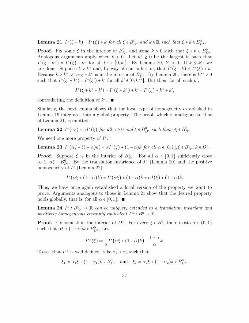
Lemma 21 I∗(ξ + k) = I∗(ξ) + k for all ξ ∈ B0D∗ and k ∈ R such that ξ + k ∈ B0

D∗.

Proof. Fix some ξ in the interior of B0D∗ and some k > 0 such that ξ + k ∈ B0

D∗ .Analogous arguments apply when k < 0. Let k∗ ≥ 0 be the largest k′ such thatI∗(ξ + k′′) = I∗(ξ) + k′′ for all k′′ ∈ [0, k′]. By Lemma 20, k∗ > 0. If k ≤ k∗, weare done. Suppose k > k∗ and, by way of contradiction, that I∗(ξ + k) ≠ I∗(ξ) + k.Because k > k∗, ξ′ ∶= ξ + k∗ is in the interior of B0

D∗ . By Lemma 20, there is k∗∗ > 0such that I∗(ξ′ + k′) = I∗(ξ′) + k′ for all k′ ∈ [0, k∗∗]. But then, for all such k′,

I∗(ξ + k∗ + k′) = I∗(ξ + k∗) + k′ = I∗(ξ) + k∗ + k′,

contradicting the definition of k∗.

Similarly, the next lemma shows that the local type of homogeneity established inLemma 19 integrates into a global property. The proof, which is analogous to thatof Lemma 21, is omitted.

Lemma 22 I∗(γξ) = γI∗(ξ) for all γ ≥ 0 and ξ ∈ B0D∗ such that γξ ∈ B0

D∗.

We need one more property of I∗.

Lemma 23 I∗(αξ + (1 − α)k) = αI∗(ξ) + (1 − α)k for all α ∈ [0,1], ξ ∈ B0D∗ , k ∈D

∗.

Proof. Suppose ξ is in the interior of B0D∗ . For all α ∈ [0,1] sufficiently close

to 1, αξ ∈ B0D∗ . By the translation invariance of I∗ (Lemma 20) and the positive

homogeneity of I∗ (Lemma 22),

I∗(αξ + (1 − α)k) = I∗(αξ) + (1 − α)k = αI(ξ) + (1 − α)k.

Thus, we have once again established a local version of the property we want toprove. Arguments analogous to those in Lemma 21 show that the desired propertyholds globally, that is, for all α ∈ [0,1].

Lemma 24 I∗ ∶ B0D∗ → R can be uniquely extended to a translation invariant and

positively homogeneous certainty equivalent I∗e ∶ B0 → R.

Proof. Fix some k in the interior of D∗. For every ξ ∈ B0, there exists α ∈ (0,1)such that αξ + (1 − α)k ∈ B0

D∗ . Let

I∗e(ξ) ∶=1

αI∗(αξ + (1 − α)k) −

1 − α

αk.

To see that I∗e is well defined, take α1 > α2 such that

ξ1 ∶= α1ξ + (1 − α1)k ∈ B0D∗ and ξ2 ∶= α2ξ + (1 − α2)k ∈ B

0D∗ .

37

By construction, ξ2 =α2

α1ξ1 + (1 − α2

α1)k. By Lemma 23, I∗(ξ2) = α2

α1I(ξ1) + (1 − α2

α1)k,

which is equivalent to

1

α1

I∗(ξ1) −1 − α1

α1

k =1

α2

I∗(ξ2) −1 − α2

α2

k.

Thus, I∗e is well defined. Messy but straight-forward calculations show that I∗e

is translation invariant. Using translation invariance and Lemma 23, one can thenshow that I∗e is positively homogeneous. By construction, I∗e is increasing andnormalized. Finally, I∗e is norm continuous because it is increasing and translationinvariant. Thus, I∗e is a certainty equivalent in the sense of Section 2.

A.2 Proof of Theorem 3

Let f ∶ U(X∞) → U(X∞) by such that f(U(d)) = U(d) for all d ∈ X∞. BecauseU, U ∶ X∞ → R represent the same preference relation on X∞, f is well defined andstrictly increasing. Because U is continuous and X∞ is connected, the set U(X∞) =

f(U(X∞)) ⊂ R is connected. Thus, f is continuous. Let z ∈X be such that (z, z, ...) ∈X∞ attains the minimum of U ∶ X∞ → R. Such a z ∈ X exists by Lemma 10.Renormalizing if necessary, assume that u(z) = 0. Let E be the set of all points inthe interior of U(X∞) at which f is differentiable. Because f is increasing, Ec hasouter measure zero. See Royden [29, Thm 3, p.100]. Moreover, for every x ∈ X,s ∈ U(X∞), and k ∈ R small enough, we have

f[u(x) + b(x)(s + k)] − f[u(x) + b(x)s]

b(x)k=b(x)

b(x)

f(s + k) − f(s)

k. (A.15)

Thus, if f is differentiable at s ∈ U(X∞), then f is differentiable at every point inthe set

A(s) ∶= u(x) + b(x)s ∶ x ∈X.

We want to show that f is differentiable at each s ∈ U(X∞). Each set A(s), s ∈ E,is an interval because X is connected and u, b ∶X → R are continuous. Also, s ∈ A(s)for every s ∈ E. Because Ec has zero measure, for every s′ in the interior of U(X∞),there is s ∈ E such that s > s′ > 0. Thus, it suffices to show that f is differentiableon (0, s] for every s ∈ E. Fix such an s and let sn ∶= b(z)ns, n ∈ N. Since u(z) = 0,sn ∈ A(s) for every n. Since s ∈ E, f is differentiable at every sn. Also,

sn+1 ∈ A(sn+1) ∩A(sn) ∀n. (A.16)

38

Conclude that the set ∪nA(sn) is connected. Since sn →n 0, it follows that (0, s] ⊂∪nA(sn). Since f is differentiable on every A(sn), we are done.

Next, we deduce from (A.15) that

b(x)f ′[u(x) + b(x)s] = b(x)f ′(s) ∀x ∈X,s ∈ U(X∞). (A.17)

We want to show that the derivative f ′ is never 0. By way of contradiction, supposef ′(s) = 0 for some s ∈ U(X∞). Since b(x), b(x) > 0 for all x ∈ X, it follows from(A.17) that

f ′[u(x) + b(x)s] = 0 ∀x ∈X.

Conclude that f ′(s′) = 0 for all s′ ∈ A(s). This contradicts the fact that f is strictlyincreasing.

The next step is to show that b = b. Take some x ∈X such that s ∶= u(x)(1−b(x))−1 ∈U(X∞). Plugging x and s into (A.17) gives

b(x)f ′(s) = b(x)f ′(s).

Since f ′(s) ≠ 0, we are done.

The final step is to show that f is affine. Since b = b, (A.17) becomes

f ′[u(x) + b(x)s] = f ′(s) ∀x ∈X,∀s ∈ U(X∞). (A.18)

Fix some s ∈ U(X∞) and once again let sn ∶= b(z)ns. It follows from (A.18) that f ′

is constant on each interval A(sn). As argued above, A(sn)∩A(sn+1) ≠ ∅ for every n.Also, (0, s] ⊂ ∪nA(sn). In particular, f ′ is constant on (0, s] for every s ∈ U(X∞).Conclude that f is affine on U(X∞) and, since f is continuous, that f is affine.

A.3 Proof of Theorem 2

Let Hrp be the set of all repeating permutation acts h ∈ H.

Lemma 25 U Hrp is dense in U H.

Proof. Take some act h ∈ H. Since h is finite, there is some t ∈ T and a finite partitionΠ ∶= A1, ...,An ⊂ Ft such that h is Π-adapted. Fix some ωi from each set Ai andwrite (xi0, x

i1, ...) for h(ωi) ∈ X∞. For every k ∈ T and every i, let aki ∶= (xi0, ..., x

ik).

Let bk1 ∶= (ak1, ak2, ...., a

kn), b

k2 ∶= (ak2, a

k3, ...., a

k1),..., and bkn ∶= (akn, a

k1, ..., a

kn−1). Let hk be

39

the Π-adapted act such that hk(ω) = (bki , bki , ...) for all ω ∈ Ai and i. Observe that

hk ∈ Hrp and hk →k h.

To develop intuition about the proof of Theorem 2, it is helpful to restate IHUT interms of a utility representation (u, b, I). First, we need some notation. Given t ∈ T ,write a for a list (x0, x1, ..., xt−1) ∈ X t of outcomes as well as for a list (f0, ..., ft−1)of functions from Ω into X. Then, every repeating permutation act h ∈ Hrp can bewritten as a sequence (a, a, ...) for some list a = (f0, f1, ..., ft−1) of functions and somet ∈ T . If h = (a, a, ...) is a repeating permutation act, we also know that for everyω,ω′ ∈ Ω, the lists

(f0(ω), f1(ω), ..., ft−1(ω)) ∈X t and (f0(ω′), f1(ω′), ..., ft−1(ω′)) ∈X t

are permutations of one another. Given a function b ∶X → (0,1), it follows that

Πt−1k=0 b(fk(ω)) = Πt−1

k=0 b(fk(ω′)) ∀ω,ω′ ∈ Ω.

Going back to the repeating permutation act h = (a, a, ...), we can thus let

b(a) ∶= Πt−1k=0b(fk(ω)) (A.19)

and be certain that b(a) is a number in (0,1) independent of ω ∈ Ω.

Next, suppose ⪰ is a path stationary preference relation on H with a representation(u, b, I). Let h, g,m ∈ H be as in the statement of IHUT. Since h is a repeatingpermutation act, h = (a, a, ...) for some list a of functions. Defining b(a) as in(A.19), observe that

U m = (1 − b(a))[U h] + b(a)[U g].

Moreover, IHUT becomes equivalent to the implication:

I[U h] ≥ I[U g]⇒ I((1 − b(a))[U h] + b(a)[U g]) ≥ I[U g]. (A.20)

If I is quasiconcave, then (A.20) is true by definition. On its own, (A.20) is strictlyweaker than quasiconcavity since U h is restricted to lie in the set U Hrp and sincethe mixing weight b(a) is a function of h. Our strategy is to show that the set U Hrp

is sufficiently rich for (A.20) to imply quasiconcavity. From Lemma 25, we alreadyknow that U Hrp is dense in U H. Roughly, the bulk of the remaining proof is toshow that U Hrp (or some transformation thereof) contains an open set O. Then,(A.20) implies that I is quasiconcave within O and, since I is homogeneous, that Iis quasiconcave.

To state the next lemma, fix a repeating permutation act (a, a, ...) ∈ Hrp and somex ∈X .

40

Lemma 26 If (a, a, ...) ∼ (x,x, ...), then (a, x, a, x, ...) ∼ (x,x, ...).

Proof. Let h ∶= (a, x, a, x, ...). First, we are going to show that h ⪰ (x,x, ...). ByPS, (x, a, a, a, ...) ∼ (x,x, ...) ∼ (a, a, ...). By IHUT, (a, x, a, a, a, ...) ⪰ (a, a, ...). ByPS again,

(x, a, x, a, a, a, ...) ⪰ (x, a, a, ...) ∼ (a, a, ...).

By IHUT again, (a, x, a, x, a, a, a, ...) ⪰ (a, a, ...). Repeating the argument and usingthe fact that ⪰ is continuous shows that h ⪰ (x,x, ...). By way of contradiction, sup-pose now that h ≻ (x,x, ...). Then, h ≻ (x,h) ≻ (x,x, ...). But (x,h) = (x, a, x, a, ...),that is, (x,h) is a repeating permutation act. By IHUT, we conclude that (x, a, h) ⪰(x,h). By PS, (a, h) ⪰ h and, hence, (a, h) ≻ (x,x, ...). The latter implies that(a, h) ≻ (x, a, h). To summarize, we have

(a, h) ≻ (x, a, h) ⪰ (x,h) = (x, a, x, a, ...).

By IHUT again, (x, a, a, h) ⪰ (x,h). By PS, (a, a, h) ⪰ h. Similarly, (a, a, a, h) ⪰ h.Iterating the argument and using the fact that ⪰ is continuous, we deduce that(a, a, ...) ⪰ h. Altogether, we have

(a, a, ...) ⪰ h ≻ (x,x, ...) ∼ (a, a, ...),

a contradiction.

Next, let Π ⊂ ∪tFt be a finite partition of Ω. To complete the proof of Theorem 2,it is enough to show that I is positively homogeneous and quasiconcave when I isrestricted to the space of Π-measurable functions in B0. Based on PS, it is w.l.o.g.to assume that Π ⊂ F1. To simplify the exposition, we also assume that Π containsthree sets so that Π = A1,A2,A3. The arguments extend naturally to all finitepartitions Π.

Assume that utility is normalized so that 0 ∈ u(X). Let x0 ∈ X be such thatu(x0) = 0 and let β ∶= b(x0). Fix some (y0, y1, y2) ∈X3 and consider the Π-measurablefunctions f0, f1, ..., f11 from Ω into X defined as

f3 ∶ x0 x0 y0 f7 ∶ y1 x0 x0 f11 ∶ x0 y2 x0f2 ∶ x0 y0 x0 f6 ∶ x0 x0 y1 f10 ∶ y2 x0 x0f1 ∶ y0 x0 x0 f5 ∶ x0 y1 x0 f9 ∶ x0 x0 y2f0 ∶ x0 x0 x0 f4 ∶ x0 x0 x0 f8 ∶ x0 x0 x0

− − − − − − − − −

A1 A2 A3 A1 A2 A3 A1 A2 A3

41

Let

a ∶= (f0, f1, ..., f11)

h ∶= (a, a, ...)

h′ ∶= (a, x0, x0, ...)

b(y0, y1, y2) ∶= b(y0)b(y1)b(y2)β9.

Thus defined, h is a repeating permutation act and

U h =1

1 − b(y0, y1, y2)U h′.

As we vary the choice of (y0, y1, y2) ∈X3, we obtain different acts h and h′. Let Hrp3be the space of all repeating permutation acts h obtained in this manner. Also, letΦ be the function

(y0, y1, y2)↦ U h′.

Since each function U h′ ∶ Ω → R is Π-measurable, we can identify U h′ with avector in R3. Then, Φ becomes a function from X3 into R3.

Lemma 27 Φ(X3) has nonempty interior in R3. In particular, 0 ∈ Φ(X3).

Proof. By construction,

β−1Φ(y0, y1, y2) =

⎡⎢⎢⎢⎢⎢⎣

1 β5b(y0) β7b(y0)b(y1)β β3b(y0) β8b(y0)b(y1)β2 β4b(y0) β6b(y0)b(y1)

⎤⎥⎥⎥⎥⎥⎦

⎡⎢⎢⎢⎢⎢⎣

u(y0)u(y1)u(y2)

⎤⎥⎥⎥⎥⎥⎦

.

If we let v0 ∶= u(y0), v1 ∶= b(y0)u(y1) and v2 ∶= b(y0)b(y1)u(y2), we can rewrite theabove expression as

β−1Φ(y0, y1, y2) =

⎡⎢⎢⎢⎢⎢⎣

1 β5 β7

β β3 β8

β2 β4 β6

⎤⎥⎥⎥⎥⎥⎦

⎡⎢⎢⎢⎢⎢⎣

v0v1v2

⎤⎥⎥⎥⎥⎥⎦

The 3 × 3 matrix in the last expression has full rank. Hence, the linear mapping

L(v0, v1, v2) ∶=

⎡⎢⎢⎢⎢⎢⎣

1 β5 β7

β β3 β8

β2 β4 β6

⎤⎥⎥⎥⎥⎥⎦

⎡⎢⎢⎢⎢⎢⎣

v0v1v2

⎤⎥⎥⎥⎥⎥⎦

42

from R3 into R3 maps open sets into open sets. Now, consider the set

C ∶= (u(y0), b(y0)u(y1), b(y0)b(y1)u(y2)) ∶ (y0, y1, y2) ∈X3

Let b ∶= minx∈X b(X) ∈ (0,1). The latter is well defined since the function b ∶ X →

(0,1) is continuous and X is compact. Let B0 ∶= u(X),B1 ∶= bu(X), and B2 ∶=

b2u(X). Note that B0 × B1 × B2 is a rectangle in R3 with nonempty interior. Wewish to show that B0 ×B1 ×B2 ⊂ C. Take any (v0, v1, v2) ∈ B0 ×B1 ×B2. Let y0 ∈ Xbe such that u(y0) = v0. Recall that utility is normalized so that 0 ∈ u(X). Thus,by construction,

v1 ∈ B1 = bu(X) ⊂ b(y0)u(X).

Hence, we can find y1 ∈X such that v1 = b(y0)u(y1). Similarly,

v2 ∈ B2 = b2u(X) ⊂ b(y0)b(y1)u(X).

Hence, we can find y2 ∈X such that v2 = b(y0)b(y1)u(y2). Conclude that B0×B1×B2 ⊂

C. Hence, L(B1 ×B2 ×B3) ⊂ Φ(X3). Since B0 ×B1 ×B2 has nonempty interior andL maps open sets into open sets, Φ(X3) ≠ ∅. By construction, 0 ∈ [B1 ×B2 ×B3]

and, hence, 0 ∈ Φ(X3).

Next, consider the mapping

Γ(y0, y1, y2) ∶=1

1 − b(y0, y1, y2)Φ(y0, y1, y2).

Note that Γ(X3) = U Hrp3 and recall that we identify U H

rp3 with a subset of R3.

Focus on the restriction of I to R3. The remainder of the proof is broken in twocases.

Case 1: Suppose b ∶ X → (0,1) is constant so that b(x) = β for every x ∈ X.Then, Γ = (1 − β12)−1Φ, implying that Γ(X3) has nonempty interior in R3 and0 ∈ O ∶= Γ(X3).

Lemma 28 I is positively homogeneous.

Proof. Suppose by way of contradiction that I is not positively homogeneous.Then, we can find ξ ∈ O and α ∈ (0,1) such that I(ξ) = 0 but I(αξ) ≠ 0. SinceI is continuous, there is α′ ∈ (α,1] such that I(α′ξ) = 0 and I(α′′ξ) ≠ 0 for allα′′ ∈ [α,α′). But since α′ξ ∈ O, there is some repeating permutation act h ∈ H

rp3

such that U h ∶= α′ξ. Adopting the notation used in Lemma 26, write h as a

43

sequence (a, a, ...) where a is some finite list of Π-measurable functions f ∶ Ω → X.Let g1 ∶= (a, x0, a, x0, ...), g2 ∶= (a, a, x0, a, a, x0, ...), and so on. By construction, thesequence (gn)n converges pointwise to h. For every n, a direct calculation shows thatU gn = αnU h for some αn ∈ (0,1) and αn n 1. Hence, for some n large enough,α′αn ∈ [α,α′] so that I(U gn) ≠ 0. But Lemma 26 implies that I(U gn) = 0 forevery n, a contradiction.

Lemma 29 I is quasiconcave.

Proof. Suppose not. Since I is positively homogeneous, we can find ξ, ξ′ ∈ O andγ ∈ (0,1) such that I(ξ) = I(ξ′) = 0 and I(γξ + (1 − γ)ξ′) < 0. Since I is continuous,we can also choose ξ and ξ′ such that the preceding inequality obtains for everyγ ∈ (0,1). Since ξ, ξ′ ∈ O = U H

rp3 , there are repeating permutation acts h and h′

such that U h = ξ and U h′ = ξ′. IHUT implies that I(γξ + (1 − γ)ξ′) ≥ 0 for someγ ∈ (0,1), a contradiction.

Case 2: Suppose b ∶X → (0,1) is nonconstant. Theorem 1 shows that I is positivelyhomogeneous. It remains to show that I is quasiconcave.21 By way of contradiction,suppose there are ξ, ξ′ ∈ U H and γ ∈ (0,1) such that I(ξ) = 0, I(ξ′) > 0, andI(γξ′ + (1 − γ)ξ) < 0. Since I is continuous, we can assume that the inequality holdsfor all γ in some interval (0, γ) ⊂ (0,1). Since I is continuous and U Hrp is dense inU H, we can also assume that ξ′ ∈ U Hrp. From Lemma 27, we know that the rayS extending from 0 ∈ R3 and passing through ξ′ intersects the open set Φ(X3) ∋ 0.Thus, we can find a sequence (yn0 , y

n1 , y

n2 )n such that Φ(yn0 , y

n1 , y

n2 ) ∈ S for every n and

Φ(yn0 , yn1 , y

n2 )→n 0 ∈ R3. Let

ξn ∶=1

1 − b(yn0 , yn1 , y

n2 )

Φ(yn0 , yn1 , y

n2 )

λn ∶= 1 − b(yn0 , yn1 , y

n2 )

Since b(X) ⊂ (0,1), the λn are bounded away from 0 and 1, that is, there is ε > 0such that λn ∈ [ε,1 − ε] ⊂ (0,1) for each n. Since Φ(yn0 , y

n1 , y

n2 ) →n 0, it follows that

ξn →n 0. By construction, each ξn lies on the ray through ξ′. Hence, ξn = knξ′

for some kn > 0. Also, kn →n 0. Since I is positively homogeneous, we know thatI(ξn) = knI(ξ′) > 0 = I(ξ). For each n, there is a repeating permutation act hn ∈ H

rp3

21If one could once again show that Γ(X3) has nonempty interior, then Lemma 29 would deliver thedesired result. When b ∶ X → (0,1) is non-constant however, we have not been able to prove thatthe interior of Γ(X3) is nonempty. Hence, we provide a different argument for the quasiconcavityof I.

44

such that U hn = ξn. By IHUT,

0 ≤ I(λnξn + (1 − λn)ξ) = I(λnknξ′ + (1 − λn)ξ) ∀n. (A.21)

Let αn ∶=λnkn

λnkn+(1−λn) . Since I is positively homogeneous, (A.21) implies that

0 ≤ I(αnξ′ + (1 − αn)ξ) ∀n. (A.22)

Recall that kn →n 0, while the sequence (λn)n is bounded away from 1. Thus, αn →n

0. But then (A.22) contradicts the fact that I(γξ′+(1−γ)ξ) < 0 for all γ in the open in-terval (0, γ).

References

[1] C. Aliprantis and K. Border. Infinite Dimensional Analysis. Springer-Verlag, 2edition, 1999. A.1.3

[2] S. Alon and D. Schmeidler. Purely subjective maxmin expected utility. Journalof Economic Theory, 152:382–412, 2014. 7.1

[3] D. K. Backus, B. R. Routledge, and S. E. Zin. Exotic preferences for macroe-conomists. In NBER Macroeconomics Annual, volume 19, pages 319–390. MITPress, 2004. 8

[4] A. Bommier, A. Kochov, and F. LeGrand. On monotone recursive preferences.forthcoming in Econometrica, 2016. 3.1, 7.2, 7.2, 7.3, 20

[5] R. Casadesus-Masanell, P. Klibanoff, and E. Ozdenoren. Maxmin expectedutility over Savage acts with a set of priors. Journal of Economic Theory, 92(1):35–65, 2000. 7.1

[6] S. H. Chew and L. G. Epstein. Recursive utility under uncertainty. In A. M.Khan and N. C. Yannelis, editors, Equilibrium Theory in Infinite DimensionalSpaces, volume 1 of Studies in Economic Theory, pages 352–369. Springer BerlinHeidelberg, 1991. 7.3

[7] G. Debreu. Representation of a preference ordering by a numerical utility func-tion. In R. Thrall, C. Coombs, and R. Davis, editors, Decision Processes. JohnWiley & Sons, 1954. A.1.2

[8] D. Ellsberg. Risk, ambiguity and the Savage axioms. Quarterly Journal ofEconomics, 75:643–669, 1961. 1

[9] L. G. Epstein. Stationary cardinal utility and optimal growth under uncertainty.Journal of Economic Theory, 31(1):133–152, 1983. 1, 3.1, 3.2, 4, 5, 6, 7.3

45

[10] L. G. Epstein. A simple dynamic general equilibrium model. Journal of Eco-nomic theory, 41(1):68–95, 1987. 8

[11] L. G. Epstein and J. A. Hynes. The rate of time preference and dynamic eco-nomic analysis. The Journal of Political Economy, 91(4):611–635, 1983. 1

[12] L. G. Epstein and M. Schneider. Ambiguity and asset markets. Annual Reviewof Financial Economics, 2:315–346, 2010. 1

[13] L. G. Epstein and S. Zin. Substitution, risk aversion, and the temporal behaviorof consumption and asset returns: A theoretical framework. Econometrica, 57(4):937–969, 1989. 7.3

[14] P. Ghirardato and M. Marinacci. Risk, ambiguity, and the separation of utilityand beliefs. Mathematics of operations research, 26(4):864–890, 2001. 7.1

[15] P. Ghirardato and M. Marinacci. Ambiguity made precise: A comparativefoundation. Journal of Economic Theory, 102(2):251–289, 2002. 3.1

[16] P. Ghirardato, F. Maccheroni, M. Marinacci, and M. Siniscalchi. A subjectivespin on roulette wheels. Econometrica, 71:1897–1908, 2003. 7.1

[17] P. Ghirardato, F. Maccheroni, and M. Marinacci. Differentiating ambiguity andambiguity attitude. Journal of Economic Theory, 118(2):133–173, 2004. 1

[18] I. Gilboa and D. Schmeidler. Maxmin expected utility with non-unique prior.Journal of Mathematical Economics, 18:141–153, 1989. 1, 7.1

[19] A. Kochov. Time and No Lotteries: An Axiomatization of Maxmin ExpectedUtility. Econometrica, 83(1):239–262, 2015. 1, 3, 3.1, 3.2, 4, 7.1, 7.3, A.1.1,A.1.9

[20] A. Kochov. A separation result for stationary preferences. Journal of Mathe-matical Economics, 70:123–126, 2017. 11

[21] T. Koopmans. Stationary ordinal utility and impatience. Econometrica, 28(2):287–309, 1960. 1, 3.1, 4, 7.2

[22] T. C. Koopmans, P. A. Diamond, and R. E. Williamson. Stationary utility andtime perspective. Econometrica, pages 82–100, 1964. 4

[23] D. Kreps and E. Porteus. Temporal resolution of uncertainty and dynamicchoice theory. Econometrica, 46(1):185–200, 1978. 7.4

[24] R. Lucas and N. Stokey. Optimal growth with many consumers. Journal ofEconomic Theory, 32(1):139–171, 1984. 8

[25] A. Lundberg. Cliff functions-a tool tor treating sequences of composed functions.Aequationes Mathematicae, 18:35–53, 1978. A.1.4

[26] A. Lundberg. Generalized distributivity for real, continuous functions. i: Struc-ture theorems and surjective solutions. Aequationes Mathematicae, 24(1):74–96,1982. 7.2, 7.2, 7.3, A.1.3, A.1.3, A.1.4, A.1.4, A.1.4, A.1.4, A.1.5, A.1.5

46

[27] A. Lundberg. Generalized distributivity for real, continuous functions. ii: Localsolutions in the continuous case. Aequationes Mathematicae, 28(1):236–251,1985. A.1.8, A.1.8, A.1.9, A.1.10

[28] F. Maccheroni, M. Marinacci, and A. Rustichini. Dynamic variational prefer-ences. Journal of Economic Theory, 128(1):4–44, 2006. 7.1, 7.4

[29] H. Royden. Real Analysis. Macmillan, New York, 3rd edition, 1988. A.2

[30] L. Savage. The Foundations of Statistics. Wiley, New York, NY, 1954. 2, 4

[31] T. Strzalecki. Temporal resolution of uncertainty and recursive models of am-biguity aversion. Econometrica, 81(3):1039–1074, 2013. 7.4

[32] H. Uzawa. Time preference, the consumption function, and optimum assetholdings. In Value, Capital and Growth. Aldine, Chicago, 1968. 1

47