1

STATIC RANGE ASSIGNMENT IN WIRELESS SENSOR NETWORKS

A THESIS SUBMITTED TOTHE GRADUATE SCHOOL OF NATURAL AND APPLIED SCIENCES

OFMIDDLE EAST TECHNICAL UNIVERSITY

BY

ERKAY UZUN

IN PARTIAL FULFILLMENT OF THE REQUIREMENTSFOR

THE DEGREE OF MASTER OF SCIENCEIN

COMPUTER ENGINEERING

OCTOBER 2010

Approval of the thesis:

STATIC RANGE ASSIGNMENT IN WIRELESS SENSOR NETWORKS

submitted by ERKAY UZUN in partial fulfillment of the requirements for the degree of Mas-ter of Science in Computer Engineering Department, Middle East Technical Universityby,

Prof. Dr. Canan OzgenDean, Graduate School of Natural and Applied Sciences

Prof. Dr. Adnan YazıcıHead of Department, Computer Engineering

Prof. Dr. Adnan YazıcıSupervisor, Computer Engineering Dept., METU

Examining Committee Members:

Assoc. Prof. Dr. Ahmet CosarComputer Engineering Dept., METU

Prof. Dr. Adnan YazıcıComputer Engineering Dept., METU

Asst. Prof. Dr. Ibrahim KorpeogluComputer Engineering Dept., Bilkent University

Asst. Prof. Dr. Sinan KalkanComputer Engineering Dept., METU

Dr. Cevat SenerComputer Engineering Dept., METU

Date: 01.10.2010

I hereby declare that all information in this document has been obtained and presentedin accordance with academic rules and ethical conduct. I also declare that, as requiredby these rules and conduct, I have fully cited and referenced all material and results thatare not original to this work.

Name, Last Name: ERKAY UZUN

Signature :

iii

ABSTRACT

STATIC RANGE ASSIGNMENT IN WIRELESS SENSOR NETWORKS

Uzun, Erkay

M.Sc., Department of Computer Engineering

Supervisor : Prof. Dr. Adnan Yazıcı

October 2010, 63 pages

Energy is a limited source in wireless sensor networks and in most applications, it is non-

renewable; so designing energy-efficient communication patterns is very important. In this

thesis, we define the static range assignment (SRA) problem for wireless sensor networks,

which focuses on providing the required connectivity in the network with minimum energy

consumption. We propose minimum spanning tree based (MST), pruned minimum span-

ning tree based (MSTP) and shortest path incremental (SPI) algorithms as efficient heuristics

for the SRA problem. As a data dissemination service, multicasting is frequently used for

communication in the wireless sensor networks. In a WSN, several multicast requests occur

simultaneously. In order to support multiple multicast requests, sensor nodes should have

enough power levels for packet transmission between the nodes. In our study we present min-

imum energy multiple source multicast (MEMSM) problem. MEMSM problem is a special

case of the SRA problem and we propose the M-MIPF algorithm as a solution to the MEMSM

problem, which is a modified version of the well-known MIPF algorithm in order to support

multiple multicast problem. Solutions to MEMSM problem try to make a range assignment

that enables all the multicasts in the system and has a minimum energy cost. We compare

the algorithms MST, MSTP, SPI and M-MIPF according to their energy consumptions. Our

experimental results show that MSTP and SPI algorithms are stable and energy-efficient so-

iv

lutions to the MEMSM problem.

Keywords: Wireless Sensor Networks, Multicasting, Range Assignment, Shortest Path, Span-

ning Tree

v

OZ

KABLOSUZ ALGILAYICI AGLARDA SABIT MENZIL AYARLAMA

Uzun, Erkay

Yuksek Lisans, Bilgisayar Muhendisligi

Tez Yoneticisi : Prof. Dr. Adnan Yazıcı

Ekim 2010, 63 sayfa

Kablosuz algılayıcı aglarda enerji kısıtlı miktarda bulunmaktadır ve bircok uygulamada enerji

kaynakları yenilenebilir degildir. Bu sebepten oturu enerjiyi az kullanan haberlesme modelleri

gelistirmek cok onemlidir. Bu tezde, sabit menzil ayarlama (SRA) problemi tanımlanmaktadır.

SRA problemi en az enerji kullanarak gerekli haberlesmeyi saglama uzerine odaklanmaktadır.

SRA probleminin cozumu icin en kucuk kapsayan agac temelli (MST), kucultulmus kapsayan

agac temelli (MSTP) ve en kısa yol artıs temelli (SPI) algoritmalarını sunmaktayız. Bilgi

paketlerinin dagıtımı amacıyla coklu yayım yontemi agda haberlesmeyi saglamak icin sıklıkla

kullanılmaktadır. Bundan dolayı bir kablosuz agda bircok coklu yayım gerceklesmektedir.

Birden fazla coklu yayım istegini desteklemek ve kablosuz algılayıcılar arasında paket trans-

ferlerini saglamak icin algılayıcıların yeterli miktarda guc seviyelerinin olması gerekmektedir.

Calısmamızda en az enerji tuketen bircok coklu yayım (MEMSM) problemini tanımlıyoruz.

MEMSM problemi SRA problemini ozel bir halini teskil etmektedir. MEMSM problemi-

nin cozumu icin bilinen MIPF algoritmasının degistirilmis versiyonu olan M-MIPF algorit-

masını sunuyoruz. MEMSM problemi icin gelistirilen cozumler agdaki butun coklu yayımları

destekleyecek ve bunun yanında en az enerji harcayacak sekilde bir menzil ataması yapmayı

amaclar. Gelistirdigimiz MST, MSTP, SPI ve M-MIPF algoritmalarını enerji tuketimlerine

gore karsılastırıyoruz. Deney sonuclarımız gostermektedir ki; MEMSM problemi icin MSTP

vi

ve SPI algoritmaları kararlı ve enerji verimli cozumlerdir.

Anahtar Kelimeler: Kablosuz Algılayıcı Aglar, Coklu Yayım, Menzil Ayarlama, En Kısa Yol,

Kapsayan Agac

vii

To my family...

viii

ACKNOWLEDGMENTS

I owe my deepest gratitude to my supervisor, Prof.Dr. Adnan Yazıcı, for his encouragement,

guidance and support throughout my thesis studies.

I would like to thank to my jury members, Assoc. Prof. Dr. Ahmet Cosar, Asst. Prof. Dr.

Ibrahim Korpeoglu, Asst. Prof. Dr. Sinan Kalkan and Dr. Cevat Sener for reviewing and

evaluating my thesis.

I would also like to thank TUBITAK UEKAE / ILTAREN for deeply supporting my graduate

studies.

I am thankful to my friends Fatih Deniz, Osman Osmanlı, Fatih Gokbayrak, Metehan Aydın,

Hakkı Bagcı and Hakan Bagcı, who we have lots of fun during my studies. It is also pleasure

for me to thank many of my other colleagues for motivating me.

I am very indebted to the biggest koch ever Enver Kayaaslan for his endless assistance. He

has made available his support in a number of ways.

I thank to my altruistic wife Elif for her endless love, encouragement and understanding

throughout my thesis studies.

Finally, I would like to thank my parents and my brother for their love, support and guidance

during my whole educational life.

ix

TABLE OF CONTENTS

ABSTRACT . . . . . . . . . . . . . . . . . . . . . . . . . . . . . . . . . . . . . . . . iv

OZ . . . . . . . . . . . . . . . . . . . . . . . . . . . . . . . . . . . . . . . . . . . . . vi

ACKNOWLEDGMENTS . . . . . . . . . . . . . . . . . . . . . . . . . . . . . . . . . ix

TABLE OF CONTENTS . . . . . . . . . . . . . . . . . . . . . . . . . . . . . . . . . x

LIST OF TABLES . . . . . . . . . . . . . . . . . . . . . . . . . . . . . . . . . . . . xii

LIST OF FIGURES . . . . . . . . . . . . . . . . . . . . . . . . . . . . . . . . . . . . xiii

LIST OF ALGORITHMS . . . . . . . . . . . . . . . . . . . . . . . . . . . . . . . . . xv

LIST OF ABBREVATIONS . . . . . . . . . . . . . . . . . . . . . . . . . . . . . . . xvi

CHAPTERS

1 INTRODUCTION . . . . . . . . . . . . . . . . . . . . . . . . . . . . . . . 1

2 BACKGROUND AND RELATED WORK . . . . . . . . . . . . . . . . . . 5

2.1 Minumum Energy Broadcast Problem . . . . . . . . . . . . . . . . 9

2.1.1 Spanning Tree Algorithms . . . . . . . . . . . . . . . . . 10

2.1.2 Topology Control Algorithms . . . . . . . . . . . . . . . 12

2.1.3 Local Search Algorithms . . . . . . . . . . . . . . . . . . 13

2.2 Minumum Energy Multicast Problem . . . . . . . . . . . . . . . . . 15

3 STATIC RANGE ASSIGNMENT PROBLEM . . . . . . . . . . . . . . . . . 18

3.1 General Framework . . . . . . . . . . . . . . . . . . . . . . . . . . 18

3.2 Formal Problem Definition . . . . . . . . . . . . . . . . . . . . . . 19

3.3 Algorithms . . . . . . . . . . . . . . . . . . . . . . . . . . . . . . . 24

3.3.1 Baseline:Minimum Spanning Tree Based (MST) . . . . . 24

3.3.2 Pruned Minimum Spanning Tree Based (MSTP) . . . . . 27

3.3.3 Shortest Path Based Incremental (SPI) . . . . . . . . . . . 28

x

3.4 Discussions . . . . . . . . . . . . . . . . . . . . . . . . . . . . . . 31

4 MULTIPLE SOURCE MULTICASTING . . . . . . . . . . . . . . . . . . . 33

4.1 Multiple Source Multicasting Framework . . . . . . . . . . . . . . . 33

4.2 Formal Definition . . . . . . . . . . . . . . . . . . . . . . . . . . . 34

4.3 Combinatorial Reduction to SRA Problem . . . . . . . . . . . . . . 35

4.4 Baseline: Merging-based Range Assignment (M-MIPF) . . . . . . . 36

5 EXPERIMENTAL RESULTS . . . . . . . . . . . . . . . . . . . . . . . . . 38

5.1 Setup and Data . . . . . . . . . . . . . . . . . . . . . . . . . . . . . 38

5.2 Multiple Source Multicasting . . . . . . . . . . . . . . . . . . . . . 41

6 GUI FOR ALGORITHM VISUALIZATION . . . . . . . . . . . . . . . . . 54

7 CONCLUSION . . . . . . . . . . . . . . . . . . . . . . . . . . . . . . . . . 59

REFERENCES . . . . . . . . . . . . . . . . . . . . . . . . . . . . . . . . . . . . . . 61

xi

LIST OF TABLES

TABLES

Table 5.1 Multicast schemes generated for 50 node network topologies. . . . . . . . . 40

Table 5.2 Average normalized costs of algorithms for multicast schemes M(10, 10),

M(10, 20) and M(10, 100) . . . . . . . . . . . . . . . . . . . . . . . . . . . . . . 45

Table 5.3 Average normalized costs of algorithms for multicast schemes M(20, 10),

M(20, 20) and M(20, 100) . . . . . . . . . . . . . . . . . . . . . . . . . . . . . . 48

Table 5.4 Average normalized costs of algorithms for multicast schemes M(100, 10),

M(100, 20) and M(100, 100) . . . . . . . . . . . . . . . . . . . . . . . . . . . . 51

xii

LIST OF FIGURES

FIGURES

Figure 2.1 Wireless multicast advantage property. . . . . . . . . . . . . . . . . . . . 9

Figure 2.2 BIP uses wireless multicast advantage. . . . . . . . . . . . . . . . . . . . 12

Figure 2.3 Sweep procedure. . . . . . . . . . . . . . . . . . . . . . . . . . . . . . . 14

Figure 3.1 A sample deployment of sensor nodes illustrating a static range of a node. . 19

Figure 3.2 A sample figure illustrating locations of the nodes, distances between nodes

and range of a node. . . . . . . . . . . . . . . . . . . . . . . . . . . . . . . . . . 20

Figure 3.3 A sample (a) static range assignment and (b) corresponding range graph. . 21

Figure 3.4 A sample range graph that satisfies pair set P = {(3, 8), (1, 7)} and does not

satisfy pair set P = {(5, 8), (4, 3)} . . . . . . . . . . . . . . . . . . . . . . . . . . 22

Figure 3.5 A sample wireless sensor network with 8 nodes. . . . . . . . . . . . . . . 25

Figure 3.6 Minimum spanning tree of sample network. . . . . . . . . . . . . . . . . . 26

Figure 3.7 Range graph after the MST algorithm is executed for range assignment. . . 26

Figure 3.8 Extracted paths for pairs in the pair set. . . . . . . . . . . . . . . . . . . . 28

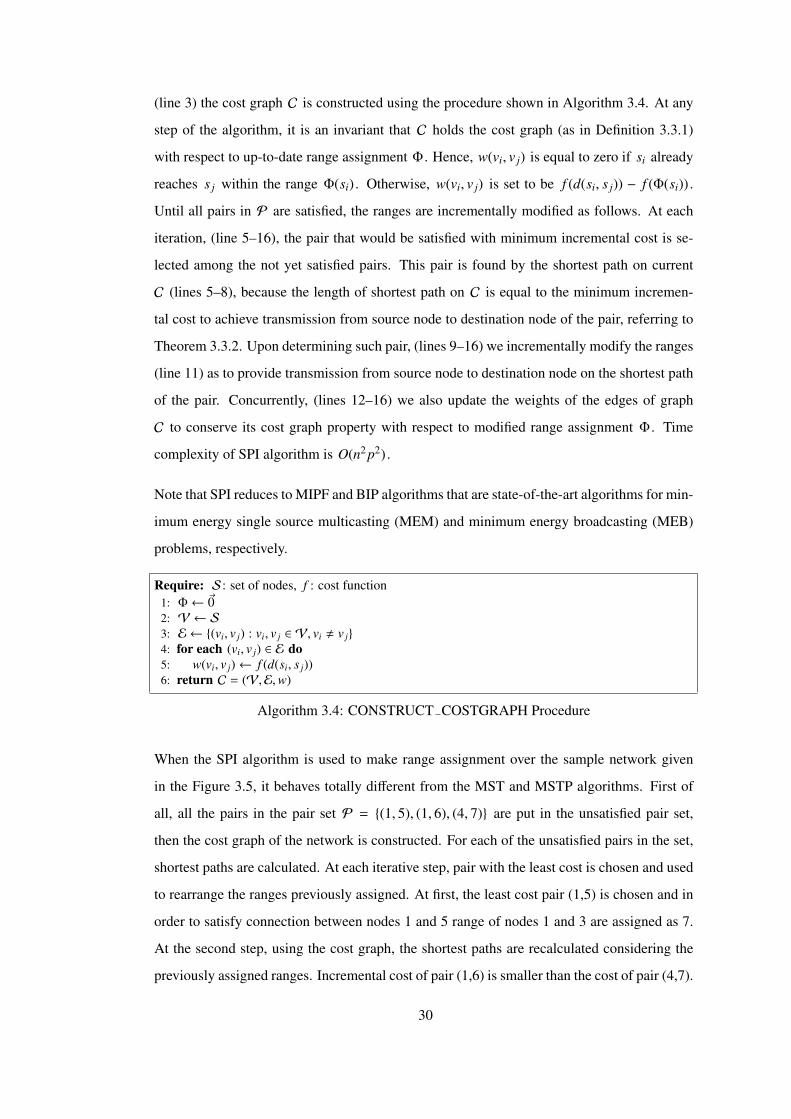
Figure 3.9 Range graph after the MSTP algorithm is executed for range assignment. . 28

Figure 3.10 Range graph after the SPI algorithm is executed for range assignment. . . . 32

Figure 4.1 A sample deployment of nodes illustrating two source multicasting with

corresponding multicasting group. . . . . . . . . . . . . . . . . . . . . . . . . . . 34

Figure 4.2 Range graph after the M-MIPF algorithm is executed for range assignment. 37

Figure 5.1 Randomly deployed 40 node sensor network. . . . . . . . . . . . . . . . . 39

Figure 5.2 Normalized costs of algorithms for Multicast schemes M(10, 10), M(10, 20)

and M(10, 100) (Top to bottom). α = 2. . . . . . . . . . . . . . . . . . . . . . . 43

xiii

Figure 5.3 Normalized costs of algorithms for Multicast schemes M(20, 10), M(20, 20)

and M(20, 100) (Top to bottom). α = 2. . . . . . . . . . . . . . . . . . . . . . . 46

Figure 5.4 Normalized costs of algorithms for Multicast schemes M(100, 10), M(100, 20)

and M(100, 100) (Top to bottom). α = 2. . . . . . . . . . . . . . . . . . . . . . . 49

Figure 5.5 Normalized costs of algorithms for Multicast schemes M(10, 10), M(20, 20)

and M(100, 100) (Top to bottom). α = 4. . . . . . . . . . . . . . . . . . . . . . . 53

Figure 6.1 Main Screen. . . . . . . . . . . . . . . . . . . . . . . . . . . . . . . . . . 54

Figure 6.2 A sample network topology with 30 nodes and seed value 17. . . . . . . . 55

Figure 6.3 Node ranges of a sample range assignment. Algorithm is SPI and network

has 30 nodes. . . . . . . . . . . . . . . . . . . . . . . . . . . . . . . . . . . . . . 57

Figure 6.4 Path graph of a sample range assignment. Algorithm is SPI and network

has 30 nodes. . . . . . . . . . . . . . . . . . . . . . . . . . . . . . . . . . . . . . 57

Figure 6.5 Path graph and node ranges of a sample range assignment. Algorithm is

SPI and network has 30 nodes. . . . . . . . . . . . . . . . . . . . . . . . . . . . 58

xiv

LIST OF ALGORITHMS

ALGORITHMS

Algorithm 3.1 CONSTRUCT GRAPH Procedure . . . . . . . . . . . . . . . . . . . 24

Algorithm 3.2 MST-based Algorithm . . . . . . . . . . . . . . . . . . . . . . . . . . 25

Algorithm 3.3 MSTP Algorithm . . . . . . . . . . . . . . . . . . . . . . . . . . . . . 27

Algorithm 3.4 CONSTRUCT COSTGRAPH Procedure . . . . . . . . . . . . . . . . 30

Algorithm 3.5 SPI Algorithm . . . . . . . . . . . . . . . . . . . . . . . . . . . . . . 31

Algorithm 4.1 MEMSM-to-SRA Reduction . . . . . . . . . . . . . . . . . . . . . . 35

Algorithm 4.2 M-MIPF Algorithm . . . . . . . . . . . . . . . . . . . . . . . . . . . 36

xv

LIST OF ABBREVATIONS

WSN Wireless Sensor Network

MEMS Micro-Electro-Mechanical Systems

MEB Minimum Energy Broadcasting

MEM Minimum Energy Multicasting

SRA Static Range Assignment

MST Minimum Spanning Tree

MSTP Pruned Minimum Spanning Tree

SPI Shortest Path Incremental

MEMSM Minimum Energy Multiple Source Multicasting

GUI Graphical User Interface

xvi

CHAPTER 1

INTRODUCTION

Wireless sensor networks (WSN) consist of small, low-cost, low power and multifunctional

sensor nodes [1]. These small sensor nodes have different components with various func-

tions. Main components of a sensor node are sensing, data processing and communicating

units. With the recent advances in micro-electro-mechanical systems (MEMS) and wireless

communications, wireless sensor networks received high attention and many applications are

developed using WSNs. A WSN consists of very large number of nodes and these nodes

work collaboratively. Number of nodes in a wireless sensor network could be hundreds or

thousands depending on the type of application. Design of a WSN is not easy due to this large

number; a considerable effort is required.

In many civil and military applications where wireless network connectivity is needed, sen-

sor nodes are deployed and used for data sensing and communication [13]. There are two

main purposes for using WSNs in the applications, these are monitoring and tracking [30].

There are many different fields where using wireless sensor networks provide considerable

advantage. One of these areas is military applications. WSNs can be used for tracking and

monitoring enemy or allied forces in battlefield. Moreover, in different attack detection tech-

niques, sensor nodes are used to prevent threats. They are easy and fast to deploy and do not

require management after deployment. Another main area, which WSNs are widely used is

environmental applications. They are deployed to detect some catastrophes such as floods and

forest fires. Furthermore, sensor nodes make tracking the animals in the environment easier.

Different kinds of devices in a home can communicate with each other using the wireless

communication. So deploying sensor nodes for home automation is also useful [1]. Some

health areas can also benefit from WSN applications such as monitoring patients and biomed-

1

ical research [25]. Considering the wide range of applications, it can be stated that WSNs are

becoming an integral part of our lives.

In wireless networks, a wired backbone infrastructure does not exist [13]. This provides

a flexible structure to the network. Nodes in the network both acts as a router and a host

with a forwarding capability to communicate with each other. Two nodes in the network can

communicate with each other through a single hop if they are close enough; otherwise they

use some intermediate nodes for communication. In a WSN, a very large number of nodes are

deployed close to each other and their positions are not predetermined [1]. Generally, they are

randomly deployed to increase flexibility of arrangement and decrease the cost of installation.

Sensor nodes have several limitations. They can only operate in a small area, they are limited

in memory and computational capacity and they have low power batteries with a limited

life. Furthermore, in most of the applications batteries can neither be replaced nor recharged

after deployment [20] [31]. Using the batteries efficiently is very important because network

lifetime is limited with the battery energy in wireless nodes. Thus, providing efficient use

of energy in the wireless sensor networks is very crucial and energy efficieny is the most

important design issue for many communication protocols.

Collaboration of sensor nodes is very important for wireless sensor networks, because to

achieve a given task in the network, sensor nodes have to communicate with each other.

There are three types of data dissemination in wireless sensor network. These are unicasting,

broadcasting and multicasting. Multicasting is a generalization of unicasting and broadcast-

ing. In a multicast request, a source node sends the same packet to a group of host nodes

in the network. In order to achieve this task, sensor nodes should have enough power levels

for transmissions. For this purpose minimum energy multicast (MEM) and minimum energy

broadcast (MEB) problems are defined and some solutions are proposed. The main aim of

these solutions is to arrange power levels of nodes such that the energy consumption of the

network becomes minimum and the multicast source can send packets to host nodes.

In this thesis, we define the static range assignment (SRA) problem. As general characteristics

of wireless sensor networks, there is always a communication between sensor nodes. This

communication can be defined as a set of node pairs. This set contains all the source and

target nodes as pairs. A pair (s, t) in the pair set shows that there is a packet transmission

from source node s to target node t . This can be a direct transmission or can be a multi-

2

hop communication which uses some intermediate nodes for communication. Static range

assignment on a network determines the ranges of all nodes in the network. The range values

are non-negative numbers, which are smaller than or equal to the maximum ranges of nodes.

Range of a node denotes the power level of the node and nodes can make direct transmissions

to the other nodes in their ranges. If a node has a zero range than this node has no power and

could not make any packet transmission.

Static range assignment problem can be defined as finding the best range assignment that

satisfies the set of required node pairs. In order to satisfy a communication pair set, the

assigned power levels of nodes should be enough to provide connectivity between any source

target pair (s, t) in the set. The best range assignment is the one with the least cost of all

assignments satisfying the connectivity. Cost of the network is dependent to the assigned

power levels of nodes. So smaller node ranges give a better range assignment for the network.

Static range assignment problem considers the whole set together and finds a solution that

provides connectivity for all pairs in the set. It does not make a range assignment for some

of the pairs in the set and does not change the assigned ranges for some other pair set. In our

thesis, we prove that the static range assignment problem is NP-hard using the NP-hardness

of the MEB problem.

Since the static range assignment problem is NP-hard, we resort to heuristics. We propose

three different heuristic algorithms for this purpose. These are minimum spanning tree based

(MST), pruned minimum spanning tree based (MSTP) and shortest path incremental (SPI)

range assignment algorithms. MST algorithm constructs a minimum spanning tree and makes

range assignments using this spanning tree. MST algorithm is taken as a baseline in our

evaluations. The second algorithm is the MSTP algorithm. It performs an efficient pruning

technique over the MST algorithm. It reduces the ranges assigned with the MST algorithm

with pruning. But at the same time MSTP algorithm ensures that the reduced ranges continue

to satisfy the pair set. The last algorithm that we propose is SPI algorithm. The SPI algorithm

assigns ranges incrementally and uses a shortest path based approach. SPI algorithm uses the

properties of the wireless medium in order to increase the performance and to make a better

range assignment.

As we stated previously, multicasting is commonly used in wireless sensor networks for data

dissemination. So, in a WSN, several multicast requests occur for communication. In our

3

study, we deal with this situation and present some approaches to solve multiple source mul-

ticasting problem efficiently. Finding an energy efficient solution to this problem is named

as minimum energy multiple source multicasting problem (MEMSM). MEMSM problem is

a generalization of MEM problem. The difference from the MEM problem is that there can

be more than one source node in MEMSM problem and for each source node there is a mul-

ticast group, which source nodes make transmissions. On the other hand, we show that the

MEMSM problem is a special case of static range assignment (SRA) problem and we prove

that the MEMSM problem is NP-hard.

We use the proposed algorithms MST, MSTP and SPI to solve the MEMSM problem. In

addition to these algorithms we also present the M-MIPF algorithm for the MEMSM prob-

lem. M-MIPF algorithm is a modified version of the well-known MIPF [27] algorithm. MIPF

algorithm is specified for single source multicast problem and solves the MEM problem ef-

ficiently. M-MIPF algorithm behaves all the multicast requests independently and find so-

lutions to them separately. All these different solutions are used to produce a final solution

for M-MIPF algorithm. M-MIPF algorithm is a strong baseline for the MEMSM algorithm.

Totally four algorithms are presented in this thesis for MEMSM problem, which are MST,

MSTP, SPI and M-MIPF algorithms.

The rest of the thesis is organized as follows. In the next chapter we give information about

studies related to minimum energy broadcast and minimum energy multicast problems and

analyze different approaches for efficient solutions. In chapter 3, we describe the SRA prob-

lem and propose three heuristic algorithms MST, MSTP and SPI to solve SRA problem. In

this chapter, we describe these three algorithms in detail and give their pseudocodes. In chap-

ter 4, we introduce the minimum energy multiple source multicast (MEMSM) problem and

present the M-MIPF algorithm. In the fifth chapter, we evaluate our proposed algorithms and

show experimental results. In the following chapter we present our graphical user interface

developed for deploying network, creating multicast groups and running algorithms. Finally,

we conclude the thesis and discuss some possible future works.

4

CHAPTER 2

BACKGROUND AND RELATED WORK

In the design of a wireless sensor network application, there are several factors to be con-

sidered. But the primary focus is on the energy consumption [1]. Because sensor nodes are

tiny microelectronic devices that contain only limited battery power. This battery power must

be utilized in a very effective way. In most of the applications in wireless sensor networks,

recharging or replacing the battery is almost impossible [3]. This means that lifetime of the

sensor node is equal to the lifetime of the battery. In a wireless network, sensor nodes serve

as transceivers. They both receive messages from neighbor nodes and make transmissions to

their neighbor nodes. In a multi-hop communication, sensor nodes on the path of commu-

nication become the relay nodes. Hence every node in the network is very important for the

communication between nodes and for the continuity of the wireless sensor network. If some

of the sensor nodes in the system run out of battery, this will have a negative effect on the

system. In such a situation, sensor network topology changes and required paths for commu-

nication are recalculated. These side effects of exhausted nodes decrease the efficiency of the

wireless sensor network. So battery usage is a very crucial and many of the algorithms devel-

oped for wireless sensor networks take the energy efficiency into consideration and generally

make it the primary design issue.

On the other hand, in other wireless networks the situation is different. Energy efficiency is

not the primary design concern in conventional wireless networks. Because the battery can be

replaced or recharged so the node lifetime is not equal to the battery lifetime. The main aim of

these kind of wireless networks is the quality of service [1], which is defined as the accepted

measure of the service quality that network users can benefit [6]. So in wireless networks the

basic design principle can change if the network is a sensor network.

5

In a wireless sensor network, sensor nodes sense data, process information, transmit packets

to neighbor nodes and receive incoming packets. A node performs different types of op-

erations in the network. A sensor node uses its energy basically for three reasons. These

power consumption areas are sensing , communication and processing . In a wireless sensor

network, most of the energy is used for communication purposes [1]. Energy spent for sens-

ing data and processing data is much less compared to the energy spent for communication.

Hence, the energy efficiency of the wireless sensor network is mostly depends on the design

of communication protocols.

In order to decrease energy usage in a wireless network generally two control mechanisms

are used [13]:

• Power mode control: Power mode control protocols put the nodes into sleep state in

order to decrease power consumption when they are in listening mode.

• Transmission power control: Transmission power control protocols adjust transmission

ranges to manage energy consumption.

Transmission power control is mainly used in broadcasting and multicasting. These are data

dissemination services in wireless networks. Broadcasting is a one-to-all service where one

node sends its data to all the other nodes in the network. This node is called as the source node.

If the range of source node is enough to send a packet to another node in the network, it makes

just one transmission and sends the packet directly to the target node. Otherwise it uses some

other nodes as relays and sends the message to target node using these intermediate nodes.

These nodes are on the path of packet transmission. This kind of communication is called

as multi-hop communication. Another data dissemination service is multicasting, which is

generalization of broadcasting. It involves sending the same data to a group of sensor nodes

named as multicast group. In the case of broadcast, multicast group is all the nodes except

the source. Multicasting is very important in the applications, in which nodes need frequent

communication with each other. Multicasting provides nodes to exchange messages in the

network. This is a very important operation for networks with limited bandwidth and having

nodes with limited battery power [21].

Broadcast and multicast data dissemination protocols play very important role as communi-

cation services for many routing protocols. Routing protocols need multicasting to control the

6

network topology and update their states. Using the data transfers between nodes, routing pro-

tocols decide the routing paths and maintain the routings between nodes. In addition to these,

data dissemination is very important to inform other nodes about environmental changes. Be-

cause these changes would have several considerable effects on the system. Therefore data

dissemination services are very important for wireless sensor networks and designing an en-

ergy efficient algorithm for these services is very crucial in the development of wireless sensor

networks [13].

The optimization problem of finding an energy efficient solution to multicasting and broad-

casting is defined as minimum energy multicast (MEM) and minimum energy broadcast

(MEB) problems. MEM and MEB problems take lots of attention and many algorithms are

developed to solve these problems efficiently. The main aim of these algorithms is to provide

an efficient communication for the system. Selecting the transmission nodes in the multi-

cast or broadcast session and arranging their power levels are the main considerations of the

multicast or broadcast algorithms [13]. MEM and MEB problems are easy to define but find-

ing optimal solution to these problems are not so easy. It is proven that MEB problem is an

NP-hard problem [19]. MEM problem is a generalization of MEB and it is also an NP-hard

problem. Therefore, generally heuristics are defined to solve these problems.

One of the most important issues in the solution of MEB and MEM problems is wireless mul-

ticast advantage property. It is very critical for communication services. Algorithms designed

for MEB and MEM problems would consider this property in order to be a more energy effi-

cient algorithm. In a wireless medium, if a node wants to communicate with another node and

send some packets, its range must cover the other node. In other words, power of the node

must be enough to send a packet. If the distance between two nodes s and k is r and if s is

the sender and k is the receiver node, than the power needed for node s to communicate with

node k is rα , which α is the propagation loss constant that takes a value between 2 and 4. Its

value depends on the properties of the communication medium.

In a wireless network, when a node makes a transmission of a packet, this packet is received

by the neighbor nodes in the area specified with the radius of the node. This is the nature

of wireless medium if omni-directional antennas are used. However in a wired network this

packet has to be sent all the neighbor nodes separately. In a wireless medium, if the source

node s needs to send a broadcast message to the nodes in its range, the cost of this trans-

7

mission will depend on the value of the range. It is not affected by the number of nodes in

the range or their distances. Let define the pi as the power needed to reach node ki from

the source node s and k1, k2 . . . kn be the neighbors of s . Then the total power p needed to

transmit a broadcast packet from source s to all neighbors is defined as:

p = maxi=1...k

pi (2.1)

However for the wired network case the situation is totally different. The total power p

becomes the sum of all the transmission costs from node s to all neighbors. So it is defined

as:

p =

k∑i=1

pi (2.2)

Figure 2.1 shows this situation with a source node and three neighbor nodes within the range

of source. Here if the source node s wants to make a packet transmission to all the neighbors,

it needs just the power required to reach the farthest of all nodes, which is k1 . By this way the

closer nodes k2 , k3 and k4 will also be in the coverage area of the source node and any packet

transmitted to the medium will be received by these three nodes. By contrast, in the case of

wired medium, the total power is the sum of three power costs needed to make transmissions

between source s and nodes k1 , k2 , k3 and k4 . This is the nature of wireless sensor networks

and the energy reduction obtained by this way is the wireless multicast advantage property.

This property gives a big advantage to wireless networks when designing algorithms. How-

ever WMA property makes the broadcasting and multicasting problems more complicated.

For instance, the MEB and MEM problems are NP-hard [19] on the other hand, in a wired

network the same optimization problem has an easier solution.

There are several solutions to minimum energy broadcast (MEB) and minimum energy multi-

cast (MEM) problems. These solutions have different approaches and they are classified into

groups according to these approaches. In the following sections different kinds of algorithms

are mentioned as a solution to MEB and MEM problem.

8

Figure 2.1: Wireless multicast advantage property.

2.1 Minumum Energy Broadcast Problem

Minimum energy broadcast problem is a difficult optimization problem. Some exact optimal

algorithms are developed to solve this problem [8]. These algorithms are developed using

MILP models. However, these solutions are not useful in practice [13]. To find a good so-

lution to this problem, generally heuristic algorithms are used. There exists many efficient

heuristic algorithms for minimum energy broadcast energy problem. These algorithms do not

guarantee the exact optimal solution but generally executes in polynomial time. Heuristic al-

gorithms are classified into three different classes according to their design perspectives [13].

These three groups of algorithms are:

• Spanning tree algorithms

• Topology control algorithms

• Local search algorithms

In the following sub-sections, these algorithms are discussed.

9

2.1.1 Spanning Tree Algorithms

In spanning tree algorithms, main purpose is to construct a spanning tree or a very similar

structure to a spanning tree with a greedy approach. By using this tree structure all the nodes

in the network can communicate with tree links. By this way, a source node in the network

can reach all the other nodes with a multihop path over many nodes. Spanning tree algorithms

builds the tree with an iterative way by adding some new nodes at each step of the algorithm.

Building a minimum spanning tree like structure is a basic but an efficient way to solve mini-

mum energy broadcast problem. There are many proposed algorithms based on this approach.

Here we overview MST [29], BIP [29], SPT [29] and BAIP [26] algorithms.

MST algorithm is a straightforward algorithm that constructs a spanning tree based on Prim’s

MST algorithm [23]. In this algorithm the link costs between nodes are calculated as the

required power for node communication. Complexity of MST algorithm is O(n3) in general,

where n is the number of nodes in the network. If the Fibonacci heap is used in implementa-

tion then the complexity becomes O(n2) . MST algorithm is a simple algorithm and it is easy

to implement but it is not an efficient algorithm in terms of energy consumption. After the

MST algorithm is executed, the ranges assigned to the nodes are not very effective. Greater

ranges are assigned to most of the nodes than they require. So the broadcast tree needs some

pruning operation after the MST algorithm is applied. In MST algorithm link based approach

is used to construct minimum energy broadcast tree. This is an old model, and many of the

previously developed models for broadcast and multicast use link based model [10]. In a link

based model, a node has to transmit its data separately to each of its neighbors. This causes

several independent transmissions. Link based models are appropriate for wired applications

and they do not carry the properties of wireless network environments. The other model used

in communication protocols is node based model. This model uses the nature of wireless

medium. In this model, when a node makes a transmission, all the nodes in its transmission

range receive the message if omnidirectional antennas are used. Many of the currently devel-

oped algorithms for multicast and broadcast consider the properties of wireless medium and

use node based model in the design.

SPT uses a linked based approach like MST algorithm but it has a different heuristic than

MST algorithm. It constructs a shortest path tree instead of minimum spanning tree. Root of

the shortest path tree is the source node in the broadcast. In SPT algorithm, shortest paths are

10

calculated from the source node to all the other nodes in the network. Dijkstra’s algorithm [9]

is used to find the shortest paths between the nodes. Shortest paths calculated from the source

node constitute the shortest path tree. SPT is a broadcast tree because it enables the source

node to send a message to any other nodes in the network. Source node can use the calculated

shortest path to reach a specified node. It uses the Dijktra’s algorithm, so the complexity of the

SPT algorithm is O(n2) , where n is the number of nodes in the network. On the other hand,

SPT algorithm is not energy efficient, it needs some improvements like pruning or Sweep [29].

BIP algorithm is proposed by Wieselthier et al. and it uses a similar heuristic with Prim’s

MST algorithm. The aim of the algorithm is to build a minimum energy tree that reaches

all the nodes in the tree from the source node. By this way, all transmission nodes and their

power levels are determined. The energy cost of the tree is the total energy consumed by the

nodes. If the range of a node is zero, then it does not have any effect on the energy cost of the

tree. Main difference from the MST algorithm is the strategy used in adding new nodes to the

tree structure. A node based approach is used in the design of algorithm and this increases the

energy efficiency. A new node is added to the tree according to the minimum incremental cost

instead of minimum cost as in MST. Wieselthier et al. defined minimum incremental cost as

the power required to increase the range of a node to reach another node in the network.

Complexity of the BIP algorithm is O(n3) , where n is the number of nodes. BIP algorithm

makes a good range assignment to the nodes and it is more energy efficient than MST and

SPT algorithms.

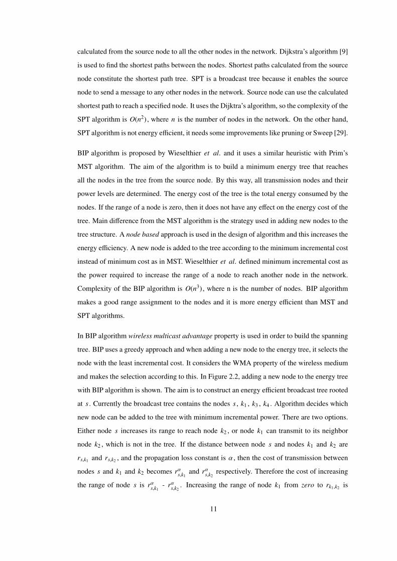
In BIP algorithm wireless multicast advantage property is used in order to build the spanning

tree. BIP uses a greedy approach and when adding a new node to the energy tree, it selects the

node with the least incremental cost. It considers the WMA property of the wireless medium

and makes the selection according to this. In Figure 2.2, adding a new node to the energy tree

with BIP algorithm is shown. The aim is to construct an energy efficient broadcast tree rooted

at s . Currently the broadcast tree contains the nodes s , k1 , k3 , k4 . Algorithm decides which

new node can be added to the tree with minimum incremental power. There are two options.

Either node s increases its range to reach node k2 , or node k1 can transmit to its neighbor

node k2 , which is not in the tree. If the distance between node s and nodes k1 and k2 are

rs,k1 and rs,k2 , and the propagation loss constant is α , then the cost of transmission between

nodes s and k1 and k2 becomes rαs,k1and rαs,k2

respectively. Therefore the cost of increasing

the range of node s is rαs,k1- rαs,k2

. Increasing the range of node k1 from zero to rk1,k2 is

11

another option to add the node k2 to the energy tree. In this example, the first option has a

lower energy cost so node s increases its range to reach k2 . BIP algorithm uses the wireless

multicast advantage property, because node s can reach both of the nodes k1 and k2 when it

transmits with sufficient power.

Figure 2.2: BIP uses wireless multicast advantage.

BAIP algorithm is a variation of BIP algorithm. It is proposed by Wan et al. . It is very

similar to BIP algorithm except that at each step more than one node can be added to the

tree. New nodes are added to the tree according to the average incremental cost metric [26].

Average incremental cost is a more general form of incremental cost approach. At each step

of the algorithm, the energy required for adding n nodes to the broadcast tree is divided by n

and average incremental cost is calculated. For each n this calculation is made and n nodes,

which give the minimum value is added to the broadcast tree.

2.1.2 Topology Control Algorithms

Topology control algorithms have a different design perspective than spanning tree algo-

rithms. In topology control algorithms, each node in the network makes its own decisions,

such as assigning range and determining transmission nodes from neighbors of a node [13].

Localized algorithms are in this group of algorithms. In localized algorithms, a node uses its

12

neighbor information to make decisions. Node can use one hop, two hop or multi hop neigh-

bor information. Some of the localized algorithms are RNG [5], LMST [17] and LBIP [14].

Minimum spanning tree (MST) is a sub graph of relative neighborhood graph (RNG). Relative

neighborhood graph can be used for broadcasting in wireless sensor networks. RNG can

be constructed using local information. It is an advantage for broadcasting problem, but it

is shown that RNG algorithms are not energy efficient [18]. Another approach to satisfy

connectivity is using minimum spanning trees. By using local network information, local

minimum spanning tree is constructed [11]. Every node uses 1-hop neighbor information

and constructs 1-hop MST. After then in the construction of LMST, these local minimum

spanning trees are used. By this way a connected structure is built with one hop neighbor

information. One of the other localized algorithms is LBIP [14], which is a localized version

of BIP. In LBIP algorithm, every node applies BIP algorithm and broadcasts its calculations.

At the end, a connected structure used for broadcasting is constructed. In LBIP algorithm two

hop neighbor information is needed.

In localized topology control algorithms, in order to construct required structures some control

messages have to be transferred between nodes in the network. If the number of messages

that flow through the network is higher, then collisions of these messages will be more. This

will cause loss of information and wrong topology construction. In addition to this, energy

consumption is also increased by the number of transferred messages. So the number of

control messages sent by nodes is a very critical issue in the design of localized topology

control algorithms.

2.1.3 Local Search Algorithms

Local search algorithms are used to improve the performance of existing MEB algorithms.

First, one of the MEB algorithms is applied to the network then a local search algorithm

is used to build a better topology. These algorithms do not change the broadcast connec-

tivity property of the network. Local search algorithms can be applied several times to the

network until no other further improvements can be done. Local search algorithms are clas-

sified into two categories. These are tree based and power assignment based local search

algorithms [13]. Tree based algorithms improves the tree structure with updates in the tree

structure in each step. In power assignment based algorithms a new power assignment is

13

made to the nodes to decrease the energy spent by nodes in the network. Here we overview

Sweep [29], EWMA [4], BIDP [11], r-shrink [7] and LESS [15] algorithms.

Sweep algorithm is proposed by Wieselthier et al. in order to improve energy efficiency

of the BIP algorithm. After the BIP algorithm is applied and tree structure is constructed,

Sweep procedure is used on the tree. It is a tree based algorithm. It finds unnecessarily

long transmission ranges and shortens them or it finds some redundant transmissions between

nodes and removes the links between these nodes. Sweep procedure is developed to increase

performance of BIP algorithm, but it can be used on any spanning tree structure. Sweep keeps

the connectivity property of the tree while making it more energy efficient. Figure 2.3 shows

broadcast tree constructed with BIP algorithm. s is the source of the energy tree. r1 and r2

are relay nodes and other nodes are the leaf nodes of the tree. Nodes r1 and r2 are in the

range of node s . s transmits broadcast packets to nodes r1 and r2 . r1 behaves as a relay and

sends the packet to nodes l1 and l2 . Similarly r2 makes transmissions to nodes l3 , l4 and l5 .

So s can make transmission to any node in the network. However this broadcast tree can be

improved with Sweep procedure. In this example the range of node s is the distance to node

r2 . It makes direct transmission to node r2 , but it is not required because node r1 can reach

to the node r2 with its current range so node s can reduce its power to reach only node r1 .

Figure 2.3: Sweep procedure.

14

BIDP makes more improvement after sweep procedure is applied on spanning tree. BIDP is

tree based search procedure like sweep. BIDP does not only remove redundant transmission

ranges, but it also reconstructs the broadcast tree by changing tree links at each iterative step

of the algorithm. It links some nodes, which are not connected and removes links between

some nodes using network topology information. At the end, broadcast tree topology changes

to a more efficient topology [13].

The r-shrink [7] is another local search procedure used to improve existing solutions for mini-

mum energy broadcast problem. It is a power assignment based algorithm. r-shrink is applied

to a node and deals with the transmissions from this node to other nodes. It shrinks the range

of the node and by this way it decreases the energy expenditure of the node when sending

messages. However when the range decreased, some of the previously reachable nodes can

become unreachable from this node. So after this shrinking operation, another parent node

must reach these nodes in order to preserve the broadcast tree topology. Shrinkage can be

applied several times until no further improvements are obtained with this procedure.

Other two local search algorithms are EWMA [4] and LESS [15]. In EWMA main purpose

is to modify the spanning tree by changing the previously assigned links. It starts from the

source node and checks if it is more advantageous to increase the power level to reach more

nodes. Range of source node increases but it can be more energy efficient if range of a

child node decreases to zero. This procedure is applied until reaching the leaf nodes of the

tree. LESS algorithm is a generalized form of EWMA. In LESS, when a node increases its

range, some of its children nodes’ ranges may decrease or reduce to zero. It can continue to

transmit with a lower range. LESS gives a better performance than EWMA, because it finds

all possible gains in the network [13].

2.2 Minumum Energy Multicast Problem

Minimum energy multicast problem is a generalization of MEB problem. In MEM problem

one node sends a packet to a previously determined group of nodes. This group is named

as multicast group. In broadcast case, this group is all of the other nodes except the sender.

So broadcast is a special case. There are many approaches to solve the minimum energy

multicast problem. To find the optimal solution to this MEM problem some MILP models are

15

developed. These models are extended versions of MILP models used in MEB problem [12].

Another way of solving this problem is defining good heuristics. These heuristic approaches

can be classified into three groups [13]. These three groups are:

• Pruning algorithms

• Minimum Steiner tree algorithms

• Local search algorithms

General approach in pruning algorithms is to prune the broadcast tree obtained by solving the

MEB problem. First one of the MEB heuristics is applied, then the required pruning operation

is executed on the connected broadcast structure. Many of the solutions to MEM problem use

pruning approach. In pruning, the nodes that do not have any children in multicast tree are

specified and their ranges are decreased to zero because there is no need for them to transmit

any messages. There are pruned versions of well-known MEB algorithms. Such as P-MST

and P-BIP where P stands for ”pruned”. P-BIP is also known as MIP [29]. In MIP algorithm

BIP algorithm is executed first, then pruning operation is started for some nodes according to

the multicast group.

Using a minimum Steiner tree is another approach to solve the MEM problem. Minimum

Steiner tree problem is to find a minimum energy multicast tree [24]. Minimum Steiner tree

construction is an NP-hard problem and there exist no optimal solution but there are some

good heuristics to solve this problem. These heuristic solutions can be used to solve the

MEM problem. The two heuristic solutions we present here are SPF and MIPF [27]. SPF

algorithm builds a tree and makes the source node as the root of the tree. Starting from the

source node, algorithm adds a group of nodes, which are on the least cost path at each iterative

step. Least cost path is selected from all the paths that are between the nodes in the tree and

the nodes not in the tree but in the multicast group. Algorithm repeats this step until all the

nodes in the multicast group are reachable. On the other hand, MIPF algorithm uses a similar

approach with the BIP algorithm. It uses wireless multicast advantage property as a difference

from the SPF algorithm. In MIPF, similar to SPF, a tree where the root is the source node is

built. At each iterative step of the algorithm, considering the minimum incremental power

property, some nodes are added to the tree structure. The nodes, which are added to tree, are

on the path with the least incremental power. The incremental energy costs of the paths are

16

calculated for the paths between the nodes in the tree and the nodes in the multicast group

but not in the tree yet. The path with the minimum energy cost becomes the least incremental

power path. Then all the nodes on this path are added to the tree structure. This procedure

continues until all the nodes in the multicast group are added to the tree.

Local search procedures are used for the same purpose they are used in MEB problem. They

can improve the solutions to MEM algorithms. Some of these algorithms are S-REMIT [28],

MIDP [11] and DMEM [22] algorithms. S-REMIT and MIDP algorithms are tree based

local search algorithms, on the other hand DMEM is power assignment based local search

algorithm. DMEM and S-REMIT are distributed and MIDP is a centralized algorithm.

S-REMIT algorithm improves the existing multicast tree that is constructed after any MEM

algorithm is executed. It changes some links in the tree to make the tree more energy efficient.

Centralized MIDP algorithm is similar to S-REMIT algorithm. It is also tree based, but it does

not use a multicast tree as an initial tree. It uses a broadcast tree and improves this tree at each

step of the algorithm. At the end, the broadcast tree turns out to a multicast tree and this tree

is the output of the algorithm. The distributed algorithm DMEM is power assignment based

and each node in the network makes its own decisions about its power level. These nodes

can be tree or non-tree nodes. Nodes give this decision by considering their distances to all

neighbors. At each step, using these calculations, total power levels assigned to nodes are

decreased. In addition to energy efficiency increase in the system, the multicast property of

the topology is conserved [13].

17

CHAPTER 3

STATIC RANGE ASSIGNMENT PROBLEM

In this chapter, we present the static range assignment (SRA) problem for wireless sensor

networks and propose three algorithms as solution to the SRA problem.

3.1 General Framework

The wireless sensor nodes are generally deployed into a field in order to sense and extract in-

formation that need to be forwarded to some other nodes. In this thesis, we study the scenario

in which some nodes multicast their information periodically. Most of the previous work on

this topic solves multicasting problem using radius assignment. For each multicast request in

the system, the power levels of the nodes are adjusted according to this new request. However

changing power levels for each multicast request is not very applicable in real systems [16].

We focus on the case that a node is not able to change its transmission range dynamically.

Thus, nodes make transmission with their predetermined range that is statically assigned be-

fore they are started to operate. However, it is possible that nodes have different transmission

ranges.

The aim is to determine such ranges for wireless sensor nodes as to ensure transmission of

messages between some source-destination pairs and minimizing the total energy consumed

or the number of transmissions. In Figure 3.1 a sample 5 node network is displayed. There

are two transmissions in this network, one is from node 2 to node 4 and the other one is from

node 1 to node 5. Node 3 is a relay node and it has to transmit packets received from nodes

1 and 2. After the static range assignment for this network, power level of node 3 should be

enough to send the farther of the two nodes, which is node 5.

18

Figure 3.1: A sample deployment of sensor nodes illustrating a static range of a node.

3.2 Formal Problem Definition

We are given a set S = {s1, s2, . . . , sn} of n nodes where each node si is associated with a

point p(si) in r -dimensional1 space Rr . The distance d(si, s j) between two nodes si and s j

is defined as the euclidean distance between the respective locations p(si) and p(s j) , i.e.,

d(si, s j) = ‖p(si) − p(s j)‖r (3.1)

Given this notation, the static range assignment (or simply, range assignment) of a set S of

nodes is defined as follows.

Definition 3.2.1 (Static Range Assignment) A static range assignment Φ : S → R+ ∪ {0}

is a function from the set S to a set of non-negative real values, where Φ(si) refers to the

assigned range of node si .

In Figure 3.2, an 8 node wireless sensor network is displayed with their specified locations. In

this figure the range of node 1 is shown as a circle with radius r . This figure also illustrates the1 r = 2 is often the case.

19

distance between two nodes. The distance between nodes 4 and 7 is drawn as a line between

nodes.

Figure 3.2: A sample figure illustrating locations of the nodes, distances between nodes andrange of a node.

Definition 3.2.2 (Range Graph) For a range assignment Φ , the range graph G(Φ) = (V,E)

is a directed graph with n vertices, where a node vi ∈ V corresponds to the node si ∈ S and

a directed edge (vi, v j) ∈ E refers to that node si can reach to node s j within the range Φ(si) .

E = {(vi, v j) : d(si, s j) ≤ Φ(si)} (3.2)

Figure 3.3, contains two small figures. Top figure shows the ranges of nodes after a sample

range assignment. At the bottom figure corresponding range graph is displayed for the same

sensor network. Range graph is a directed graph. If two of the nodes are in the range of

each other, then the arrow is two-sided. If only one of the nodes(source) covers the other

node(target), then there is an arrow from source to target node. In the figure there is no

outgoing arrow from nodes 6 and 7, which states that these nodes have zero range. They do

not make any transmissions in the network.

We are also given a non-decreasing binary function f which maps each range r ∈ R+ to a real

valued positive cost and such that f (0) = 0. The function f often refers to the energy spent

by node si during one message transmission. As a result, the cost c(Φ) of an assignment is

20

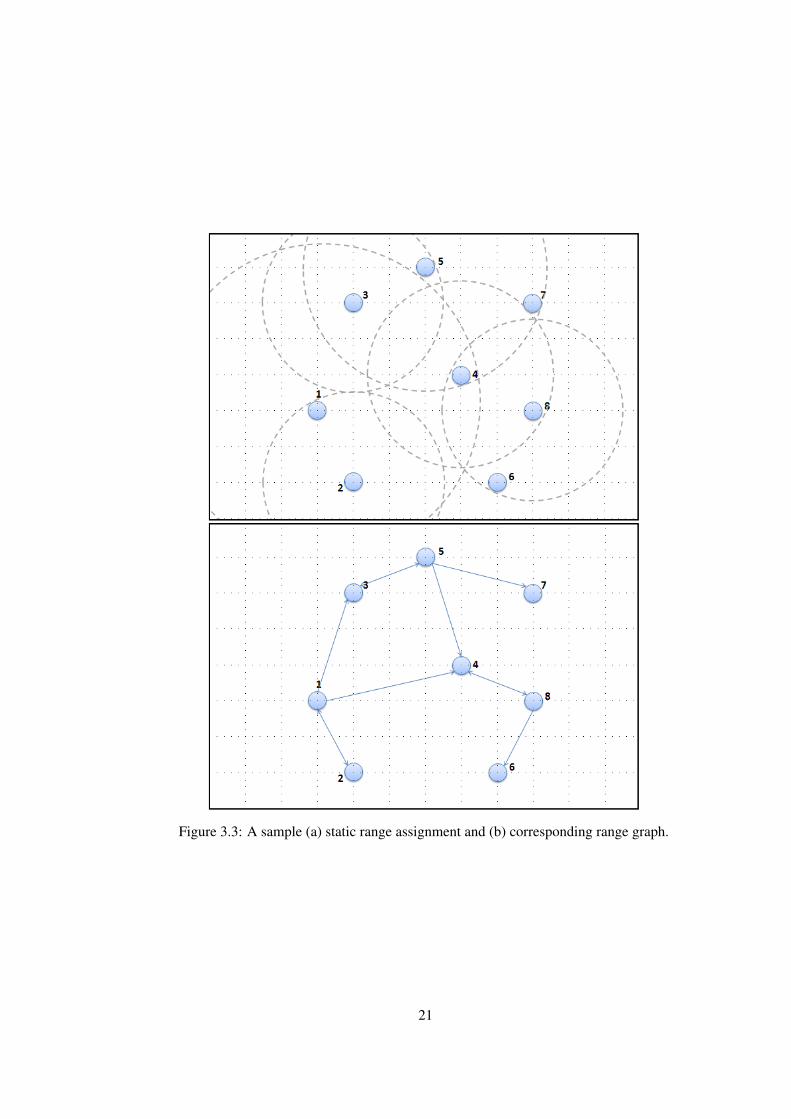
Figure 3.3: A sample (a) static range assignment and (b) corresponding range graph.

21

defined as follows:

c(Φ) =∑si∈S

f (Φ(si)) (3.3)

Finally, we are given a set P = {(si1 , s j1), (si2 , s j2), . . . , (sip , s jp)} of p pairs of nodes of S ,

where each pair (si, s j) indicates the necessity of any path from vi to v j . We say a graph G

satisfies P if for each pair (si, s j) ∈ P , there exists a path from vi to v j in G . Given all these

notations, the static range assignment problem is defined in Problem 1.

Figure 3.4 shows the same network topology and range graph with Figure 3.3. This figure

illustrates how a range graph satisfies a given pair set P . For instance the pair set P =

{(3, 8), (1, 7)} is satisfied with this graph. There exists a path from 3 to 8, which is 3 → 5 →

4→ 8. Also the path 1→ 3→ 5→ 7 used for the communication from 1 to 7. These paths

are drawn as bold in the figure. On the other hand, this range graph does not satisfy the pair

set P = {(5, 8), (4, 3)} because no path exists from 4 to 3.

Problem 1 (Static Range Assignment Problem (SRA)) Given a set S of nodes with asso-

ciated points at Rr and a set P of pair of nodes in S , find a range assignment Φ such that

the range graph G(Φ) satisfies the set P and the cost c(Φ) is minimized.

Figure 3.4: A sample range graph that satisfies pair set P = {(3, 8), (1, 7)} and does not satisfypair set P = {(5, 8), (4, 3)}

Theorem 3.2.3 Static range assignment problem is NP-hard.

22

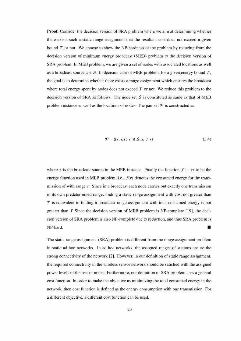
Proof. Consider the decision version of SRA problem where we aim at determining whether

there exists such a static range assignment that the resultant cost does not exceed a given

bound T or not. We choose to show the NP-hardness of the problem by reducing from the

decision version of minimum energy broadcast (MEB) problem to the decision version of

SRA problem. In MEB problem, we are given a set of nodes with associated locations as well

as a broadcast source s ∈ S . In decision case of MEB problem, for a given energy bound T ,

the goal is to determine whether there exists a range assignment which ensures the broadcast

where total energy spent by nodes does not exceed T or not. We reduce this problem to the

decision version of SRA as follows. The node set S is constituted as same as that of MEB

problem instance as well as the locations of nodes. The pair set P is constructed as

P = {(s, si) : si ∈ S, si , s} (3.4)

where s is the broadcast source in the MEB instance. Finally the function f is set to be the

energy function used in MEB problem, i.e., f (r) denotes the consumed energy for the trans-

mission of with range r . Since in a broadcast each node carries out exactly one transmission

in its own predetermined range, finding a static range assignment with cost not greater than

T is equivalent to finding a broadcast range assignment with total consumed energy is not

greater than T .Since the decision version of MEB problem is NP-complete [19], the deci-

sion version of SRA problem is also NP-complete due to reduction, and thus SRA problem is

NP-hard. �

The static range assignment (SRA) problem is different from the range assignment problem

in static ad-hoc networks. In ad-hoc networks, the assigned ranges of stations ensure the

strong connectivity of the network [2]. However, in our definition of static range assignment,

the required connectivity in the wireless sensor network should be satisfied with the assigned

power levels of the sensor nodes. Furthermore, our definition of SRA problem uses a general

cost function. In order to make the objective as minimizing the total consumed energy in the

network, then cost function is defined as the energy consumption with one transmission. For

a different objective, a different cost function can be used.

23

3.3 Algorithms

Since the static range assignment problem is NP-complete, we resort to heuristics. For this

purpose, we present three algorithms, one of which, namely minimum spanning tree based

(MST) algorithm is taken as a naive baseline. Thus, we propose two algorithms to solve SRA

problem, namely pruned minimum spanning tree based range assignment (MSTP) algorithm

and shortest path based incremental range assignment (SPI) algorithm. The former algorithm

employs an effective pruning technique over MST algorithm, whereas the latter one incre-

mentally assigns ranges conducting shortest path based approach at each step. For the sake of

simplicity in complexity calculations, we denote n and p as the number of nodes of S and

the number of paths in pair set P , respectively.

3.3.1 Baseline: Minimum Spanning Tree Based Range Assignment (MST)

Algorithm 3.1 shows the undirected graph constructing procedure, which is commonly used

by several algorithms presented in this section, from a given set of nodes (with associated

points) and cost function. Mainly, we define an edge between each (unordered) pair of nodes

with associated weight of the incurred cost of sending message within the range of the distance

in terms of given cost function. This procedure runs in O(n2) time.

Algorithm 3.2 begins with conducting an undirected graph construction over the set S of

nodes with respect to locations and cost function f . Subsequently, a minimum spanning tree

algorithm is performed to construct a rooted tree T . Upon this, the ranges of nodes assigned

such as to ensure that each node can reach both its parent (except root) and its children.

Complexity of MST algorithm is O(n2) .

Require: S : set of nodes, f : cost function1: Φ← ~02: V ← S3: E ←

(V

2

)4: for each {vi, v j} ∈ E do5: w(vi, v j)← f (d(si, s j))6: return G = (V,E,w)

Algorithm 3.1: CONSTRUCT GRAPH Procedure

Figure 3.5 shows a sample network of 8 nodes. The numbers on the edges show the distance

24

Require: S : set of nodes, P : set of pairs, f : cost function1: Φ← ~02: G ← CONSTRUCT GRAPH(S, f )3: T ← MINIMUM SPANNING TREE(G)4: for each vi ∈ T do5: v j ← T .parent[vi]6: if Φ(si) < d(si, s j) then7: Φ(si)← d(si, s j)8: if Φ(s j) < d(si, s j) then9: Φ(s j)← d(si, s j)

10: return Φ

Algorithm 3.2: MST-based Algorithm

Figure 3.5: A sample wireless sensor network with 8 nodes.

between nodes. In this network there should be connection between nodes (1,5), (1,6) and

(4,7). This means the pair set P = {(1, 5), (1, 6), (4, 7)} will be satisfied with the range graph

of the assignment. When the MST algorithm is used as a solution, it first constructs the

network graph, than finds the minimum spanning tree of the network and makes the range

assignment ensuring that the range of nodes are enough to reach children and parent nodes.

Figure 3.6 shows the constructed minimum spanning tree and Figure 3.7 shows the range

graph after assignment. MST algorithm assigns ranges greater than zero to all the nodes in

the network even some of the nodes are not used in the transmissions as a source or relay

node. For example node 2 and node 6 have ranges of 8 and 6 respectively, however they are

leaf nodes and these ranges are redundant.

25

Figure 3.6: Minimum spanning tree of sample network.

Figure 3.7: Range graph after the MST algorithm is executed for range assignment.

26

3.3.2 Pruned Minimum Spanning Tree Based Range Assignment (MSTP)

As Algorithm 3.2 performs, Algorithm 3.3 also constructs an undirected graph using the pro-

cedure defined in Algorithm 3.1 at the beginning. Discrepantly, Algorithm 3.3 assigns ranges

more effectively. Since the aim is to ensure a good transmission performance between some

particular pairs, the ranges of nodes are assigned such as message transmission can be per-

formed between those source-destination pairs using the constructed tree T as an overlay

network. That is, consider a source-destination pair which has exactly one path over T ,

which we refer here as source-destination path. The range assignment is performed such that

nodes can reach successive nodes on any such source-destination paths. MSTP algorithm runs

in O(n2 + np) time.

Require: S : set of nodes, P : set of pairs, f : cost function1: Φ← ~02: G ← CONSTRUCT GRAPH(S, f )3: T ← MINIMUM SPANNING TREE(G)4: for each pk = (ak, bk) ∈ P do5: Pk ← EXTRACT PATH(T , ak, bk)6: for each (vi, v j) ∈ Pi do7: if Φ(si) < d(vi, v j) then8: Φ(si)← d(vi, v j)9: return Φ

Algorithm 3.3: MSTP Algorithm

When the MSTP algorithm is used as a solution to the sample network given in the Figure 3.5,

as similar to MST algorithm it first constructs the network graph, than finds the minimum

spanning tree of the network. However MSTP algorithm uses an efficient pruning tecnique

over the MST algorithm. It extracts the paths for each pair in the pair set and uses these paths

for range assignment. Figure 3.8 shows the extracted paths in the network. After all the paths

are determined in the network, ranges of nodes are assigned using the paths passing over the

nodes. There do not exist any paths passing over the nodes 2 and 6 so their assigned ranges are

0. However with the MST algorithm their ranges are 8 and 6 respectively. In addition to these

improvements, some node ranges can also be decreased when compared to MST algorithm.

For instance there is just one path passing over node 1 and it should provide connectivity

of this path. MST algorithm assigns a range of 8, however 7 is enough for communication.

Figure 3.9 also shows the range graph after assignment. This range graph shows that there is

a good energy improvement over the MST algorithm, when compared to the range graph of

MST algorithm.

27

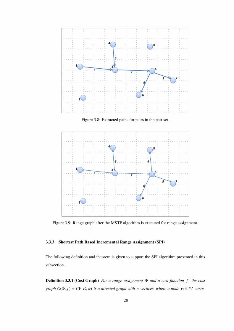
Figure 3.8: Extracted paths for pairs in the pair set.

Figure 3.9: Range graph after the MSTP algorithm is executed for range assignment.

3.3.3 Shortest Path Based Incremental Range Assignment (SPI)

The following definition and theorem is given to support the SPI algorithm presented in this

subsection.

Definition 3.3.1 (Cost Graph) For a range assignment Φ and a cost function f , the cost

graph C(Φ, f ) = (V,E,w) is a directed graph with n vertices, where a node vi ∈ V corre-

28

sponds to the node si ∈ S and the weight of a directed edge w(vi, v j) refers to that how much

additional cost necessary to be incurred to make si reach to s j , i.e.,

w(vi, v j) =

f (d(si, s j)) − f (Φ(si)) Φ(si) < d(si, s j)

0 o.w.(3.5)

Theorem 3.3.2 For a given set S of nodes, cost function f , a range assignment Φ and a

pair (a, b) of nodes, the minimum total incremental cost that should be incurred such that

range graph G(Φ) satisfies (a, b) is equal to the length of the shortest path from a to b in

cost graph C(Φ, f ) .

Proof. A minimum total increment cost should be lead by a minimal increment of ranges, i.e.,

no less increment of all ranges will lead to satisfy (a, b) . Consider a minimal increment of

ranges of nodes such as (a, b) is satisfied by G(Φ′) where Φ′ denotes the range assignment

that become after the increments. Because of the minimality each node, whose range is to be

incremented, has to reach a node that was not previously reached. This implies an edge in the

cost graph. Thus, each minimal increment of ranges induces a path in cost graph with length

same as the total increment cost. Counterside, each path in cost graph induces a minimal

increment of ranges with cost same as the length of the path. Therefore, the minimum total

incremental cost that should be incurred such that range graph G(Φ) satisfies (a, b) is equal

to the length of the shortest path from a to b in cost graph C(Φ, f ) . �

Corollary 3.3.3 For a given set S of nodes, cost function f and a range assignment Φ , G(Φ)

satisfies a pair (a, b) of nodes if and only if shortest path from a to b in C(Φ, f ) is equal to

0.

Algorithm 3.4 shows the cost graph constructing procedure that is similar to Algorithm 3.1,

where the main difference is that the edges are directed. We define an edge between each

distinct pair of nodes with associated weight of the incurred cost of sending message within

the range of the distance in terms of given cost function.

SPI, which is presented in Algorithm 3.5, is the most sophisticated heuristic among the ones

presented in this section. At the beginning, (line 2) a set of yet-unsatisfied pairs is constructed.

Since, all initial assigned ranges are zero, all pairs of P are unsatisfied. Immediately after,

29

(line 3) the cost graph C is constructed using the procedure shown in Algorithm 3.4. At any

step of the algorithm, it is an invariant that C holds the cost graph (as in Definition 3.3.1)

with respect to up-to-date range assignment Φ . Hence, w(vi, v j) is equal to zero if si already

reaches s j within the range Φ(si) . Otherwise, w(vi, v j) is set to be f (d(si, s j)) − f (Φ(si)) .

Until all pairs in P are satisfied, the ranges are incrementally modified as follows. At each

iteration, (line 5–16), the pair that would be satisfied with minimum incremental cost is se-

lected among the not yet satisfied pairs. This pair is found by the shortest path on current

C (lines 5–8), because the length of shortest path on C is equal to the minimum incremen-

tal cost to achieve transmission from source node to destination node of the pair, referring to

Theorem 3.3.2. Upon determining such pair, (lines 9–16) we incrementally modify the ranges

(line 11) as to provide transmission from source node to destination node on the shortest path

of the pair. Concurrently, (lines 12–16) we also update the weights of the edges of graph

C to conserve its cost graph property with respect to modified range assignment Φ . Time

complexity of SPI algorithm is O(n2 p2) .

Note that SPI reduces to MIPF and BIP algorithms that are state-of-the-art algorithms for min-

imum energy single source multicasting (MEM) and minimum energy broadcasting (MEB)

problems, respectively.

Require: S : set of nodes, f : cost function1: Φ← ~02: V ← S3: E ← {(vi, v j) : vi, v j ∈ V, vi , v j}

4: for each (vi, v j) ∈ E do5: w(vi, v j)← f (d(si, s j))6: return C = (V,E,w)

Algorithm 3.4: CONSTRUCT COSTGRAPH Procedure

When the SPI algorithm is used to make range assignment over the sample network given

in the Figure 3.5, it behaves totally different from the MST and MSTP algorithms. First of

all, all the pairs in the pair set P = {(1, 5), (1, 6), (4, 7)} are put in the unsatisfied pair set,

then the cost graph of the network is constructed. For each of the unsatisfied pairs in the set,

shortest paths are calculated. At each iterative step, pair with the least cost is chosen and used

to rearrange the ranges previously assigned. At first, the least cost pair (1,5) is chosen and in

order to satisfy connection between nodes 1 and 5 range of nodes 1 and 3 are assigned as 7.

At the second step, using the cost graph, the shortest paths are recalculated considering the

previously assigned ranges. Incremental cost of pair (1,6) is smaller than the cost of pair (4,7).

30

Require: S : set of nodes, P : set of pairs, f : cost function1: Φ← ~02: U ← P3: C ← CONSTRUCT COSTGRAPH(S, f )4: while U , ∅ do5: for each pi = (ai, bi) ∈ U do6: S (pi)← SHORTEST PATH(C, ai, bi)7: if w(S (pi)) < w(S (pmin)) then8: pmin = pi9: for each (vi, v j) ∈ S (pmin) do

10: if Φ(si) < d(vi, v j) then11: Φ(si)← d(vi, v j)12: for each vk ∈ V s.t. vk , vi do13: if d(vi, vk) < Φ(si) then14: w(vi, vk)← 015: else16: w(vi, vk)← f (d(si, sk)) − f (Φ(si))17: return Φ

Algorithm 3.5: SPI Algorithm

So the pair (1,6) is chosen. In order to satisfy connection between nodes 1 and 6, increasing

the range of node 3 from 7 to 8 is enough. Here we see the benefit of using wireless multicast

advantage property. After this assignment, both the pairs (1,5) and (1,6) becomes satisfied.

Only the pair (4,7) remains in the unsatisfied pair set. At the last step, this pair is chosen and

the ranges 6 and 3 are assigned to the nodes 4 and 5. SPI algorithm assigns range 3 to the

node 5, on the other hand the MSTP algorithm assigns 6. Figure Figure 3.10 shows the range

graph after the assignment. SPI algorithm performs better than the MSTP algorithm for this

sample range assignment example, because it does not use the underlying minimum spanning

tree structure and uses the advantages of wireless medium.

3.4 Discussions

Here, a quite general definition is given for static range assignment from both cost function

f and pair set P perspective. That is, this problem definition and proposed solutions can be

applied to scenarios where arbitrary cost functions are conducted and/or pair set is restricted

to have some criteria. By performing proper reductions, we can solve more specific problems.

However, one should be careful on the objective. The objective of SRA problem is determined

by the sum of individual costs of assigned ranges. Thus, the objective correctly captures of

the objective of a problem, only if nodes perform equal number of transmissions.

31

Figure 3.10: Range graph after the SPI algorithm is executed for range assignment.

Another issue is about cost function f . If function f is given as to capture the consumed

energy of a transmission, then the objective relates to minimizing total consumed energy.

Whereas, in case of that f is a binary function referring to existence of a transmission, i.e.,

r > 0, the objective reduces to minimizing number of transmitter nodes.

32

CHAPTER 4

MULTIPLE SOURCE MULTICASTING

In this chapter, we define the multiple source multicasting problem (MEMSM) and propose

an algorithm as a solution to MEMSM problem.

4.1 Multiple Source Multicasting Framework

Single source multicast is a typical scenario for wireless sensor networks. Here, we study

the case where the number of multicast tasks can be more than one. The multiple multi-

casting tasks can be considered independent. However, the nodes make transmissions with

their predetermined static ranges, that is, it is not possible to modify the range for different

multicasting tasks. Thus, the multicasting tasks are related in sense of static range assignment.

We assume that after deploying to field, each wireless sensor node operates as follows. Upon

receiving a message from other nodes, it relays the message with its predetermined range

only if both the range is greater than zero and the message is not relayed previously by the

sensor node. In order to check whether the same message is sent before, each sensor node

maintains its own list containing the identifications of previously relayed messages. For the

sake of being identical, each message is identified by its owner node’s id concatenated with

the number of messages previously originated by the owner node.

Figure 4.1 shows a multiple source multicast scenario. In this network there are two multicast

groups. First multicast group contains nodes 1,4 and 5. Source node of this group is 1. The

other multicast group has nodes 5,4,2 and 3. This group has the source node 5. Source

nodes 1 and 5 make transmissions to nodes in the multicast groups. In figure this situation is

illustrated.

33

Figure 4.1: A sample deployment of nodes illustrating two source multicasting with corre-sponding multicasting group.

4.2 Formal Definition

Minimum energy multiple source multicasting (MEMSM) problem is a more general version

of minimum energy multicasting (MEM) problem, where there does not have to be unique

source, that is more than one multicast source nodes with different groups to multicast their

data are allowed. Whereas, MEMSM problem is a special case of static range assignment

(SRA) problem (see Chapter 3) in a sense that the range cost function f is given such that

f (r) corresponds to the consumed energy per transmission within the range r . Given such

f function, the cost c(Φ) of SRA problem captures the total consumed energy for one trans-

mission per node. However, nodes can make more than one transmissions. This objective

exactly corresponds to minimizing energy in multiple source multicasting scenario, under the

assumption that each node performs a transmission within its predetermined range for each

multicasting task, i.e, for each multicast source. Otherwise, the SRA objective approximates

the objective of MEMSM problem.

In MEMSM problem, we are given a set S of nodes and their associated points. A multicast-

ing task mi is shown by a pair mk = (sk, {s1k , s

2k , . . . , s

nkk }) meaning that node vi multicasts to

a set γk = {s1k , s

2k , . . . , s

nkk } ⊂ S of nodes. For a range assignment Φ , the total consumed en-

ergy E(Φ) is taken as the cumulative energy consumptions of each transmission. The energy

34

consumed by a transmission within a range r is defined with following formula:

e(r) =

rα + ce r > 0

0 r = 0(4.1)

Problem 2 (Minimum Energy Multiple Source Multicasting (MEMSM)) Given a set S

of nodes with associated points at Rr and a set M = {m1,m2, . . .} of multicasting tasks of

nodes in S , find a range assignment Φ such that the total consumed energy E(Φ) is mini-

mized.

Theorem 4.2.1 MEMSM problem is NP-hard.

Proof. We prove the NP-hardness of MEMSM problem by reduction from minimum energy

broadcast (MEB) problem which is known to be NP-hard [19]. Broadcasting is a special case

of multicasting where the group size is equal to all nodes but the source node and there exists

single source node. That is, if s is the broadcast source, then the set M of multicasting tasks

is constructed as

M = {m1 = {s,S − {s}}} (4.2)

Upon this transformation, minimizing objective of MEMSM problem in constructed MEMSM

instance corresponds to minimizing objective of MEB problem for given MEB instance. Since

MEB is NP-hard, we conclude that MEMSM is also NP-hard. �

4.3 Combinatorial Reduction to Static Range Assignment Problem

As to solve MEMSM problem, we use combinatorial reduction to static range assignment

(SRA) problem as follows.

Require: S : set of nodes, M : set of multicast tasks1: P ← ∅2: for each mk = (sk, γk) ∈ M do3: for each s j ∈ γk do4: P ← P ∪ {(vk, v j)}5: Φ← SRA(S,P, f )6: return Φ

Algorithm 4.1: MEMSM-to-SRA Reduction

35

As seen in Algorithm 4.1, for each multicasting task mk = (sk, γk) , we introduce paths in

P from source node sk to each node in respective multicast group γk . This reduction is

exact in sense that minimization objective of SRA problem for constructed instance correctly

corresponds to minimizing the total consumed energy of given MEMSM energy under the

assumption that for each multicasting task, every node performs transmission uniquely. Once,

such reduction is constructed, it is possible to employ proposed algorithms for SRA problem.

Thus, we use MST algorithm as a baseline, whereas MSTP and SPI algorithms are considered

as novel ones in order to solve MEMSM problem.

4.4 Baseline: Merging-based Range Assignment (M-MIPF)

Here, the modified version of known MIPF [27] algorithm is presented which is referred as

M-MIPF. The MIPF algorithm is modified as to capture multiple source scenario as follows.

As also seen in Algorithm 4.2, we first treat the multicasting tasks independently and for each

multicasting task, we perform individual range assignment using MIPF which is an algorithm

specified for single source multicasting. Afterwards, the individual ranges are merged as to

ensure performance of all multicasting tasks by setting a sensor node’s range as the maximum

of the individual ranges assigned for each multicasting task. M-MIPF is happened to be the

strong baseline of MEMSM problem among the proposed algorithms. M-MIPF algorithm has

a time complexity of O(n2 p) , where p is equal to |γ1| + |γ2| + . . . |γk| .

Require: S : set of nodes, M : set of multicast tasks1: Φ← ~02: for each mk = (sk, γk) ∈ M do3: Φk ← MIPF(S, sk, γk)4: for each si ∈ S do5: if Φ(si) < Φk(si) then6: Φ(si)← Φk(si)7: return Φ

Algorithm 4.2: M-MIPF Algorithm

The M-MIPF algorithm is also used for range assignment over the wireless sensor network

given in Figure 3.5. The pair set P = {(1, 5), (1, 6), (4, 7)} contains two different multicast

requests. The source nodes are 1 and 4. One multicast request is from 1 to 5 and 6, the

other is from 4 to 7. The M-MIPF algorithm treats these two different multicasting tasks

independent from each other and makes individual range assignments using MIPF algorithm.

36

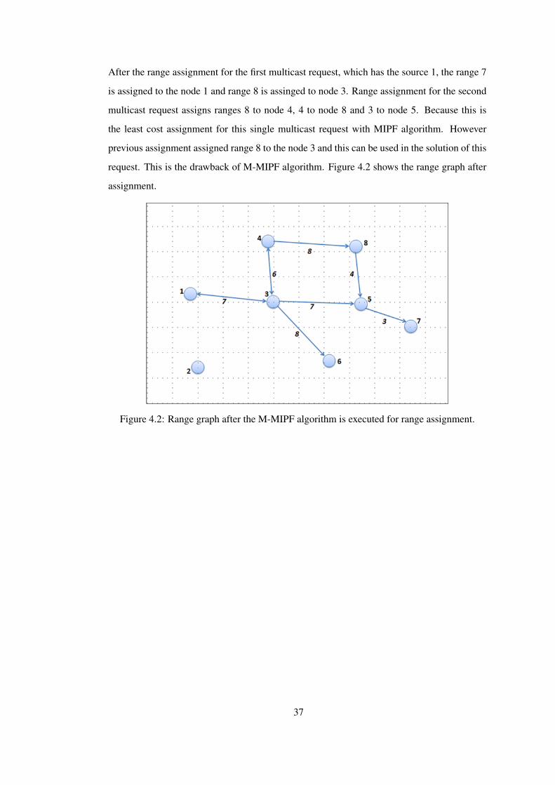
After the range assignment for the first multicast request, which has the source 1, the range 7

is assigned to the node 1 and range 8 is assinged to node 3. Range assignment for the second

multicast request assigns ranges 8 to node 4, 4 to node 8 and 3 to node 5. Because this is

the least cost assignment for this single multicast request with MIPF algorithm. However

previous assignment assigned range 8 to the node 3 and this can be used in the solution of this

request. This is the drawback of M-MIPF algorithm. Figure 4.2 shows the range graph after

assignment.

Figure 4.2: Range graph after the M-MIPF algorithm is executed for range assignment.

37

CHAPTER 5

EXPERIMENTAL RESULTS

In this chapter, we discuss the experimental results of the algorithms that are presented in

the previous chapters. We evaluate these algorithms and compare them with each other. In

the experimental process, we use many network instances as inputs to algorithms. We create

random network topology instances with different node numbers in a square region. In addi-

tion to network instances, multicast groups are determined for each of the network instances.

The transmission powers of nodes are not limited to a fixed number. Any node can make

transmission to another node in the network. So the max ranges of the nodes are not less than

the distance between the farthest nodes in the network. This chapter has two sections. In

the first section the setup procedure is given in detail. This procedure includes preparing the

data required for algorithms. Creation of network topology instances and multicast groups

are discussed in this part. In addition, the performance measures of algorithms and the way of

execution is given. In the second section, results of algorithms are given for multiple source

multicasting. Different inputs are used in the execution of algorithms. Results are displayed

with graphics for a better illustration. Comparison of algorithms and their evaluations are also

done in this part.

5.1 Setup and Data

Two main data generation processes are required for the execution of algorithms. First one

is deploying network topology instances where the algorithms are executed. The other one is

creating the multicast groups and determining their sizes and source nodes. Several network

instances are used for evaluation of algorithms. Node numbers of created network instances

are varied from 10 to 100. The value set of network node number is 10, 20 . . . 100 and 10

38

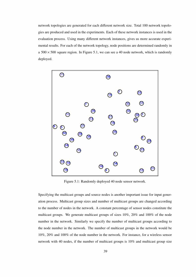
network topologies are generated for each different network size. Total 100 network topolo-

gies are produced and used in the experiments. Each of these network instances is used in the

evaluation process. Using many different network instances, gives us more accurate experi-

mental results. For each of the network topology, node positions are determined randomly in

a 500 × 500 square region. In Figure 5.1, we can see a 40 node network, which is randomly

deployed.

Figure 5.1: Randomly deployed 40 node sensor network.

Specifying the multicast groups and source nodes is another important issue for input gener-

ation process. Multicast group sizes and number of multicast groups are changed according

to the number of nodes in the network. A constant percentage of sensor nodes constitute the

multicast groups. We generate multicast groups of sizes 10%, 20% and 100% of the node

number in the network. Similarly we specify the number of multicast groups according to

the node number in the network. The number of multicast groups in the network would be

10%, 20% and 100% of the node number in the network. For instance, for a wireless sensor

network with 40 nodes, if the number of multicast groups is 10% and multicast group size

39

is 20% of the sensor node number in the network, then there is 4 multicast groups with 8

nodes. There are 10 different network sizes and 3 different multicast group sizes and 3 differ-

ent multicast group numbers. A total of 3 × 3 = 9 different multicast schemes are generated

for each network size. These schemes are applied on every network instances and used in the

execution of the algorithms. In Table 5.1, generated schemes for node number 50 are listed.

Table 5.1: Multicast schemes generated for 50 node network topologies.

Multicast Number of MulticastScheme Multicast Groups Group Size

Scheme 1 5 5Scheme 2 5 10Scheme 3 5 50Scheme 4 10 5Scheme 5 10 10Scheme 6 10 50Scheme 7 50 5Scheme 8 50 10Scheme 9 50 50

Performance measure of the algorithms is defined as the total power of multicast or broadcast

trees constructed as a solution to MEMSM problem. This total power is the sum of all the

power levels of the transmitting nodes in the network. Nodes with zero transmission power

do not have any effect on the total power. They do not make any packet transmissions or do

not behave as relay nodes in any other transmissions. Range of a node specifies the required

power level of the node. So assigning smaller ranges to nodes will produce a more energy

efficient multicast/broadcast tree. So algorithms with a better range assignment will have a

better performance over others.

Algorithms are executed for each of the network instances generated. We compare the per-

formance of the algorithms for each 9 multicast schemes. We define M(x, y) as the multicast

scheme where the number of multicast groups is x% and multicast group size is y% of all the

nodes in the network. Furthermore for each network topology, we define Ci(n,M(x, y)) as the

cost of multicast tree with number of nodes n and multicast scheme M(x, y) , generated with

algorithm i .

There are 10 network topologies with the same node number n . For an algorithm i and

multicast scheme M(x, y) these 10 different network instances are executed separately. After

40

these executions, geometric averages of results are calculated. This average value gives the

actual cost of an algorithm with a specified node number and multicast scheme.

In our evaluation of algorithms we use normalized costs of algorithms to provide a better

understanding about the results. We take the MST algorithm as a baseline and normalize any

of the other algorithms with the performance of MST. We define normalized cost as:

C′i (n,M(x, y)) =Ci(n,M(x, y))

CMS T (n,M(x, y))(5.1)

Normalized costs give us the performance of an algorithm compared to MST algorithm.

Therefore comparing the power consumptions of any of four algorithms at the same time

becomes easier.

The size of the square region (500 × 500) where the network is deployed does not affect the

performance results of the algorithms. If the size increases by a factor of n , then the distances

between nodes also increase by the same factor. So for the propagation loss constant α ,

the total power consumption of an algorithm increases by a factor nα . Therefore the actual

costs of algorithms change but all of the algorithms are affected with the same amount; the

normalized values of algorithms do not change.

We generate performance graphics after the execution of algorithms. In our graphics, the x

axis shows the node number and y axis shows the normalized energy cost of the algorithm

with the multicast scheme. The aim of these graphics is to compare the performance of

4 algorithms with specified multicast scheme. Using these graphics, the performances can

also be compared with different node numbers. For each node number there are 10 different

network topologies. In the performance graphics, the geometric average costs of network

instances are displayed. In the following section the performances of algorithms are explained

in detail.

5.2 Multiple Source Multicasting

MST, MSTP, SPI and M-MIPF algorithms are executed for the multicast schemes M(10, 10),

M(10, 20) and M(10, 100). In these multicast schemes, number of multicast groups are 10%

of the node number. On the other hand, multicast group sizes change for each multicast

41

scheme. For the first scheme, size of multicast group is 10% of the node number. For the sec-

ond and third schemes this ratio becomes 20% and 100% respectively. Propagation constant

is taken as α = 2. The execution results of the algorithms are displayed in Figure 5.2.

In Figure 5.2 we can see performance of the algorithms for three different multicast schemes.

Top graphic shows the performance of the algorithms for multicast scheme M(10, 10). For

small sensor node numbers, SPI and M-MIPF algorithms almost have the same performance.

However, if node number exceeds 30, SPI algorithm provides a better performance than MST,

MSTP and M-MIPF algorithms. This advantage does not change as the node number in-

creases in the network. For small sensor node numbers, M-MIPF algorithm performs better

than the MSTP algorithm and it has a similar performance with SPI algorithm. However when

node number increases it loses this advantage and becomes the worse of these three algo-

rithms. For networks containing more than 80 nodes the cost of M-MIPF algorithm becomes

larger than MST algorithm. On the other hand, MSTP algorithm has a worse performance

than the SPI algorithm for almost all network sizes but its performance does not decrease

dramatically like M-MIPF algorithm as the node number increases.

In the middle graphic, performances of the algorithms for the multicast scheme M(10, 20)

are displayed. Algorithms have a similar performance for the M(10, 20) multicast scheme,

which they show for the multicast scheme M(10, 10). Again the best algorithm is the SPI

algorithm. It gives the minimum cost for all node numbers. For this multicast scheme, The

M-MIPF algorithm again has a performance decrease when the node number exceeds 30. If

node number is bigger than 70, the performance of M-MIPF algorithm is even worse than the

MST algorithm. The MSTP algorithm has a lower cost performance than the SPI algorithm

but it is more efficient than the M-MIPF algorithm for this multicast scheme.

The bottom graphic shows the case when multicast group size is equal to the number of nodes

in the network. This means all the multicasts are broadcasts. Again the number of multicast

groups is 10% of the node number in the network. In this graphic it is seen that the normalized

costs of algorithms are higher when compared to the previous cases for small node number. In

the above two graphics the normalized costs are below 0.5 for small node numbers, however

for this multicast scheme normalized costs of all three algorithms are higher than 0.6. The

reason for this is the size of multicast groups. In the case of large multicast groups, more

sensor nodes become transmitters, so the energy consumption in networks increases. This

42

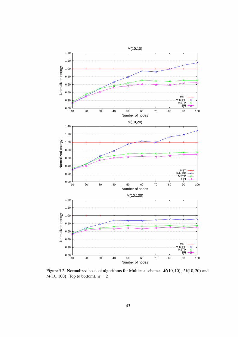
0.00

0.20

0.40

0.60

0.80

1.00

1.20

1.40

10 20 30 40 50 60 70 80 90 100

Nor

mal

ized

ene

rgy

Number of nodes

M(10,10)

MSTM-MIPF

MSTPSPI

0.00

0.20

0.40

0.60

0.80

1.00

1.20

1.40

10 20 30 40 50 60 70 80 90 100

Nor

mal

ized

ene

rgy

Number of nodes

M(10,20)

MSTM-MIPF

MSTPSPI

0.00

0.20

0.40

0.60

0.80

1.00

1.20

1.40

10 20 30 40 50 60 70 80 90 100

Nor

mal

ized

ene

rgy

Number of nodes

M(10,100)

MSTM-MIPF

MSTPSPI

Figure 5.2: Normalized costs of algorithms for Multicast schemes M(10, 10), M(10, 20) andM(10, 100) (Top to bottom). α = 2.

43

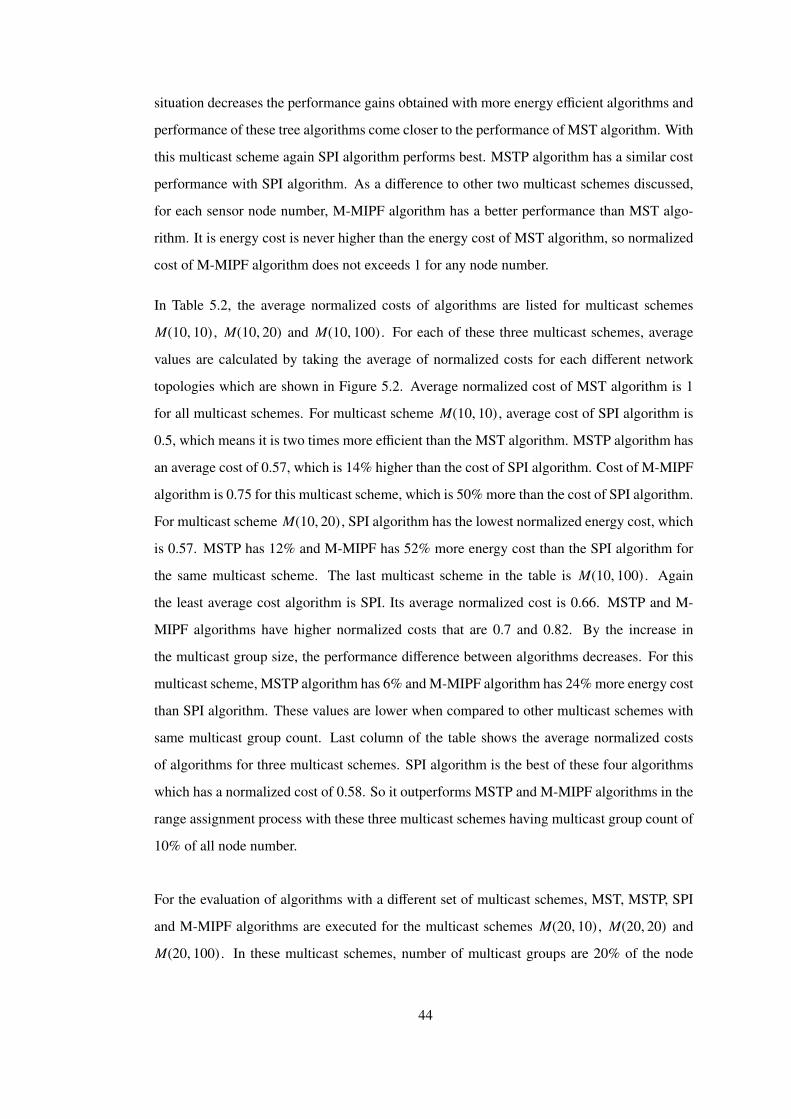
situation decreases the performance gains obtained with more energy efficient algorithms and

performance of these tree algorithms come closer to the performance of MST algorithm. With

this multicast scheme again SPI algorithm performs best. MSTP algorithm has a similar cost

performance with SPI algorithm. As a difference to other two multicast schemes discussed,

for each sensor node number, M-MIPF algorithm has a better performance than MST algo-

rithm. It is energy cost is never higher than the energy cost of MST algorithm, so normalized

cost of M-MIPF algorithm does not exceeds 1 for any node number.

In Table 5.2, the average normalized costs of algorithms are listed for multicast schemes

M(10, 10), M(10, 20) and M(10, 100). For each of these three multicast schemes, average

values are calculated by taking the average of normalized costs for each different network

topologies which are shown in Figure 5.2. Average normalized cost of MST algorithm is 1

for all multicast schemes. For multicast scheme M(10, 10), average cost of SPI algorithm is

0.5, which means it is two times more efficient than the MST algorithm. MSTP algorithm has

an average cost of 0.57, which is 14% higher than the cost of SPI algorithm. Cost of M-MIPF

algorithm is 0.75 for this multicast scheme, which is 50% more than the cost of SPI algorithm.

For multicast scheme M(10, 20), SPI algorithm has the lowest normalized energy cost, which

is 0.57. MSTP has 12% and M-MIPF has 52% more energy cost than the SPI algorithm for

the same multicast scheme. The last multicast scheme in the table is M(10, 100). Again

the least average cost algorithm is SPI. Its average normalized cost is 0.66. MSTP and M-

MIPF algorithms have higher normalized costs that are 0.7 and 0.82. By the increase in

the multicast group size, the performance difference between algorithms decreases. For this

multicast scheme, MSTP algorithm has 6% and M-MIPF algorithm has 24% more energy cost

than SPI algorithm. These values are lower when compared to other multicast schemes with

same multicast group count. Last column of the table shows the average normalized costs

of algorithms for three multicast schemes. SPI algorithm is the best of these four algorithms

which has a normalized cost of 0.58. So it outperforms MSTP and M-MIPF algorithms in the

range assignment process with these three multicast schemes having multicast group count of

10% of all node number.

For the evaluation of algorithms with a different set of multicast schemes, MST, MSTP, SPI

and M-MIPF algorithms are executed for the multicast schemes M(20, 10), M(20, 20) and

M(20, 100). In these multicast schemes, number of multicast groups are 20% of the node

44

Table 5.2: Average normalized costs of algorithms for multicast schemes M(10, 10),M(10, 20) and M(10, 100)

Average Normalized CostAlgorithm M(10, 10) M(10, 20) M(10, 100) Total Average

MSTP 0.57 0.64 0.70 0.64SPI 0.50 0.57 0.66 0.58

M-MIPF 0.75 0.87 0.82 0.81

number. On the other hand, multicast group sizes change for each multicast scheme. For the

first scheme, size of multicast group is 10% of the node number. For the second and third

schemes this ratio becomes 20% and 100%. Propagation constant is taken as α = 2. The

execution results of the algorithms are displayed in Figure 5.3.

In Figure 5.3, three graphics are displayed one for each multicast scheme. The top graphic is

for the multicast scheme M(20, 10). This multicast scheme states that multicast group count

is 20% of the node number and every multicast group has a size of 10% of the node number.

SPI algorithm has a lower energy cost than the other algorithms for all node numbers with this

multicast scheme. When the node size is smaller than 30, SPI, MSTP and M-MIPF algorithms

have a similar performance. However, when node number exceeds 30, M-MIPF algorithm

shows a dramatic increase in the energy consumption and its normalized cost becomes 1.4.

Normalized costs of SPI and MSTP algorithms never take a value bigger than 0.8.

In the middle graphic we see the results for multicast scheme M(20, 20). The performance

of the algorithms for multicast scheme M(20, 20) is similar to M(20, 10). In this scheme the

number of multicast groups does not change, but size of the multicast groups increase and

becomes 20% of all the nodes. SPI and MSTP algorithms are two most successful algorithms

with this multicast scheme. SPI algorithm performs better than all the algorithms for each

node number. Energy cost of M-MIPF algorithm is higher than the energy cost of MST

algorithm for the network topologies that have more than 40 nodes. Its normalized value

exceeds 1 in these topologies. Because the M-MIPF algorithm makes calculations for each of

the multicast schemes separately and uses these results for the overall assignment.

The bottom graphic shows the energy cost of algorithms for multicast scheme M(20, 100).

This multicast scheme denotes that all the multicast groups have 100 nodes, which means all

45

0.00

0.20

0.40

0.60

0.80

1.00

1.20

1.40

1.60

10 20 30 40 50 60 70 80 90 100

Nor

mal

ized

ene

rgy

Number of nodes

M(20,10)

MSTM-MIPF

MSTPSPI

0.00

0.20

0.40

0.60

0.80

1.00

1.20

1.40

1.60

10 20 30 40 50 60 70 80 90 100

Nor

mal

ized

ene

rgy

Number of nodes

M(20,20)

MSTM-MIPF

MSTPSPI

0.00

0.20

0.40

0.60

0.80

1.00

1.20

1.40

1.60

10 20 30 40 50 60 70 80 90 100

Nor

mal

ized

ene

rgy

Number of nodes

M(20,100)

MSTM-MIPF

MSTPSPI

Figure 5.3: Normalized costs of algorithms for Multicast schemes M(20, 10), M(20, 20) andM(20, 100) (Top to bottom). α = 2.

46

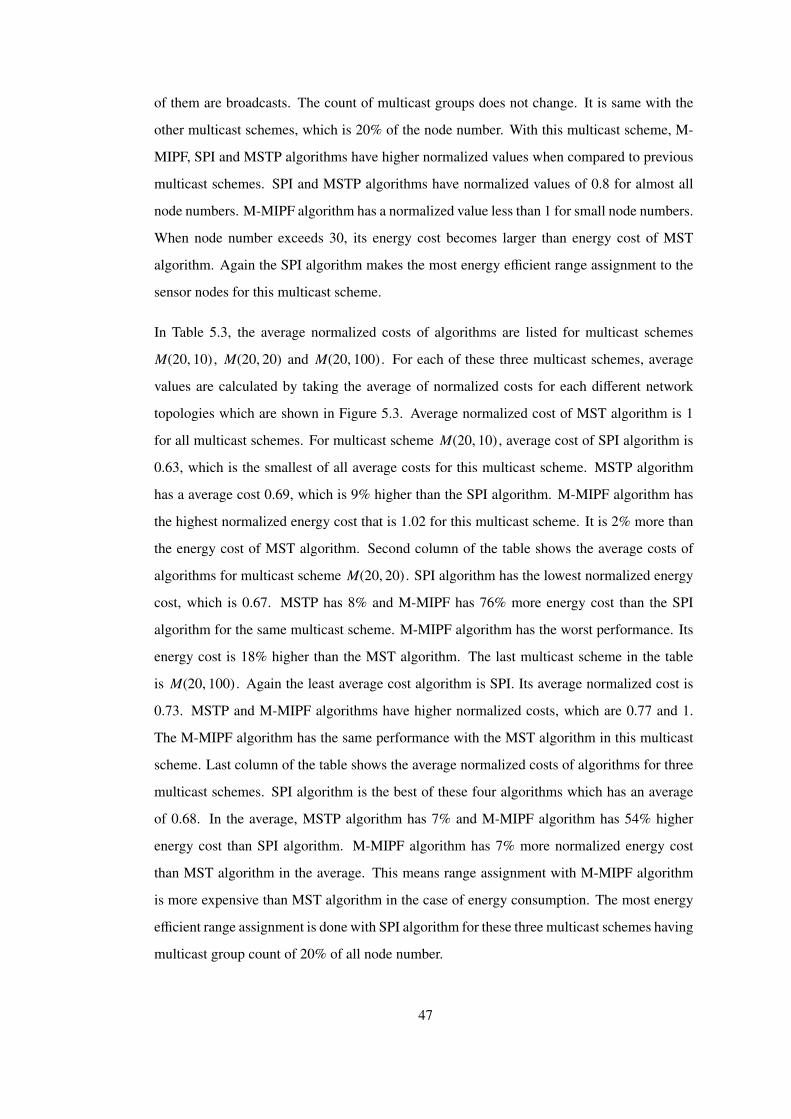
of them are broadcasts. The count of multicast groups does not change. It is same with the

other multicast schemes, which is 20% of the node number. With this multicast scheme, M-

MIPF, SPI and MSTP algorithms have higher normalized values when compared to previous

multicast schemes. SPI and MSTP algorithms have normalized values of 0.8 for almost all

node numbers. M-MIPF algorithm has a normalized value less than 1 for small node numbers.

When node number exceeds 30, its energy cost becomes larger than energy cost of MST

algorithm. Again the SPI algorithm makes the most energy efficient range assignment to the

sensor nodes for this multicast scheme.

In Table 5.3, the average normalized costs of algorithms are listed for multicast schemes

M(20, 10), M(20, 20) and M(20, 100). For each of these three multicast schemes, average

values are calculated by taking the average of normalized costs for each different network

topologies which are shown in Figure 5.3. Average normalized cost of MST algorithm is 1

for all multicast schemes. For multicast scheme M(20, 10), average cost of SPI algorithm is

0.63, which is the smallest of all average costs for this multicast scheme. MSTP algorithm

has a average cost 0.69, which is 9% higher than the SPI algorithm. M-MIPF algorithm has

the highest normalized energy cost that is 1.02 for this multicast scheme. It is 2% more than

the energy cost of MST algorithm. Second column of the table shows the average costs of

algorithms for multicast scheme M(20, 20). SPI algorithm has the lowest normalized energy

cost, which is 0.67. MSTP has 8% and M-MIPF has 76% more energy cost than the SPI

algorithm for the same multicast scheme. M-MIPF algorithm has the worst performance. Its

energy cost is 18% higher than the MST algorithm. The last multicast scheme in the table

is M(20, 100). Again the least average cost algorithm is SPI. Its average normalized cost is

0.73. MSTP and M-MIPF algorithms have higher normalized costs, which are 0.77 and 1.

The M-MIPF algorithm has the same performance with the MST algorithm in this multicast

scheme. Last column of the table shows the average normalized costs of algorithms for three

multicast schemes. SPI algorithm is the best of these four algorithms which has an average

of 0.68. In the average, MSTP algorithm has 7% and M-MIPF algorithm has 54% higher

energy cost than SPI algorithm. M-MIPF algorithm has 7% more normalized energy cost

than MST algorithm in the average. This means range assignment with M-MIPF algorithm

is more expensive than MST algorithm in the case of energy consumption. The most energy

efficient range assignment is done with SPI algorithm for these three multicast schemes having

multicast group count of 20% of all node number.

47

Table 5.3: Average normalized costs of algorithms for multicast schemes M(20, 10),M(20, 20) and M(20, 100)

Average Normalized CostAlgorithm M(20, 10) M(20, 20) M(20, 100) Total Average

MSTP 0.69 0.73 0.77 0.73SPI 0.63 0.67 0.73 0.68

M-MIPF 1.02 1.18 1.00 1.07

As a third different group of multicast schemes, MST, MSTP, SPI and M-MIPF algorithms

are executed for the multicast schemes M(100, 10), M(100, 20) and M(100, 100). In these

multicast schemes, number of multicast groups are 100% of the node number. On the other

hand, multicast group sizes change for each multicast scheme. For the first scheme, size

of multicast group is 10% of the node number. For the second and third schemes this ratio

becomes 20% and 100%. Propagation constant is taken as α = 2. The execution results of

the algorithms are displayed in Figure 5.4.

Top graphic in the Figure 5.4, shows the execution results of algorithms for the multicast

scheme M(100, 10). In this multicast scheme multicast group count is equal to the number of

nodes in the network. All the multicast groups have a size of 10% of all nodes. This means

all the nodes in the network are source nodes and makes multicast to 10 other nodes in the

network. MST, SPI and MSTP algorithms have almost same performance. Normalized costs

of SPI and MSTP algorithms are very close to 1. MST algorithm performs well with this mul-

ticast scheme because all the nodes make multicast and there are many packet transmissions

between nodes so most of the radii assigned with MST algorithm are required in commu-

nication. M-MIPF algorithm has the worst performance. As the node number increases its

normalized cost also increases. Its normalized cost is more than 2 if the node number is

greater than 60.

Middle graphic is the normalized energy cost graphic for the multicast scheme M(100, 20).

In this multicast scheme, all the nodes are transmitters, but this time the size of the multicast

groups are 20% of the node number. This graphic is similar to the previous one. For all node

numbers from 10 to 100, normalized cost of SPI and MSTP algorithms are very close to 1. M-

MIPF algorithm has the highest energy cost among these four algorithms. It is normalized cost

is never less than 1 and it performs worse than MST algorithm. Because M-MIPF algorithm

48

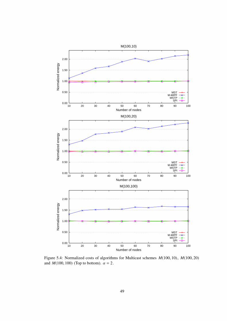
0.00

0.50

1.00

1.50

2.00

10 20 30 40 50 60 70 80 90 100

Nor

mal

ized

ene

rgy

Number of nodes

M(100,10)

MSTM-MIPF

MSTPSPI

0.00

0.50

1.00

1.50

2.00

10 20 30 40 50 60 70 80 90 100

Nor

mal

ized

ene

rgy

Number of nodes

M(100,20)

MSTM-MIPF

MSTPSPI

0.00

0.50

1.00

1.50

2.00

10 20 30 40 50 60 70 80 90 100

Nor

mal

ized

ene

rgy

Number of nodes

M(100,100)

MSTM-MIPF

MSTPSPI

Figure 5.4: Normalized costs of algorithms for Multicast schemes M(100, 10), M(100, 20)and M(100, 100) (Top to bottom). α = 2.

49

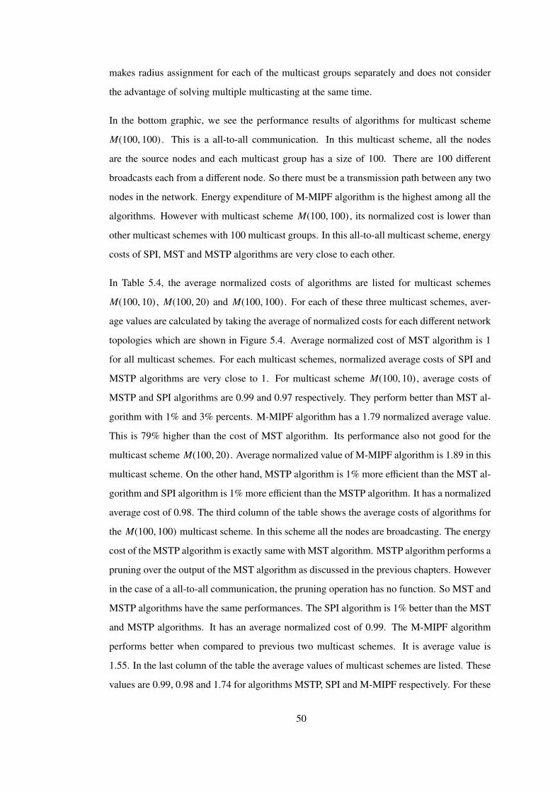
makes radius assignment for each of the multicast groups separately and does not consider

the advantage of solving multiple multicasting at the same time.

In the bottom graphic, we see the performance results of algorithms for multicast scheme

M(100, 100). This is a all-to-all communication. In this multicast scheme, all the nodes

are the source nodes and each multicast group has a size of 100. There are 100 different

broadcasts each from a different node. So there must be a transmission path between any two

nodes in the network. Energy expenditure of M-MIPF algorithm is the highest among all the

algorithms. However with multicast scheme M(100, 100), its normalized cost is lower than

other multicast schemes with 100 multicast groups. In this all-to-all multicast scheme, energy

costs of SPI, MST and MSTP algorithms are very close to each other.

In Table 5.4, the average normalized costs of algorithms are listed for multicast schemes

M(100, 10), M(100, 20) and M(100, 100). For each of these three multicast schemes, aver-

age values are calculated by taking the average of normalized costs for each different network

topologies which are shown in Figure 5.4. Average normalized cost of MST algorithm is 1

for all multicast schemes. For each multicast schemes, normalized average costs of SPI and

MSTP algorithms are very close to 1. For multicast scheme M(100, 10), average costs of

MSTP and SPI algorithms are 0.99 and 0.97 respectively. They perform better than MST al-

gorithm with 1% and 3% percents. M-MIPF algorithm has a 1.79 normalized average value.

This is 79% higher than the cost of MST algorithm. Its performance also not good for the

multicast scheme M(100, 20). Average normalized value of M-MIPF algorithm is 1.89 in this

multicast scheme. On the other hand, MSTP algorithm is 1% more efficient than the MST al-

gorithm and SPI algorithm is 1% more efficient than the MSTP algorithm. It has a normalized

average cost of 0.98. The third column of the table shows the average costs of algorithms for

the M(100, 100) multicast scheme. In this scheme all the nodes are broadcasting. The energy

cost of the MSTP algorithm is exactly same with MST algorithm. MSTP algorithm performs a

pruning over the output of the MST algorithm as discussed in the previous chapters. However

in the case of a all-to-all communication, the pruning operation has no function. So MST and

MSTP algorithms have the same performances. The SPI algorithm is 1% better than the MST

and MSTP algorithms. It has an average normalized cost of 0.99. The M-MIPF algorithm

performs better when compared to previous two multicast schemes. It is average value is

1.55. In the last column of the table the average values of multicast schemes are listed. These

values are 0.99, 0.98 and 1.74 for algorithms MSTP, SPI and M-MIPF respectively. For these

50

Table 5.4: Average normalized costs of algorithms for multicast schemes M(100, 10),M(100, 20) and M(100, 100)

Average Normalized CostAlgorithm M(100, 10) M(100, 20) M(100, 100) Total Average

MSTP 0.99 0.99 1 0.99SPI 0.97 0.98 0.99 0.98

M-MIPF 1.79 1.89 1.55 1.74

multicast schemes, which the number of multicast groups is equal to the node number, again

the SPI algorithm outperforms MSTP and M-MIPF algorithms.

We also execute algorithms with propagation loss constant α = 4. A greater α means there

is more loss in communication due to environmental conditions. So more energy is required

to make a transmission between two specified nodes when compared to α = 2 case. The ex-

ecution results of algorithms with multicast schemes M(10, 10), M(20, 20) and M(100, 100)

and α = 4 are displayed in Figure 5.5. In these multicast schemes, node number in the multi-

cast groups and size of multicast groups are equal. Top graphic shows the performance of the

algorithms for multicast scheme M(10, 10). Number of multicast groups are 10% of all the

nodes in the network in this multicast scheme. Multicast group size of each multicast group

is also equal to 10% of the node number. In this case, SPI algorithm performs best among all

of the algorithms. MSTP has a lower energy cost than M-MIPF algorithm. As a difference

from the α = 2 case, the M-MIPF algorithm performs better and its normalized cost never

exceeds 1. This means it is efficient than the MST algorithm for all node numbers. For the

multicast scheme M(20, 20), change in the α value does not make a considerable effect on

the performances of SPI and MSTP algorithms. Their normalized costs take a value close

to 0.8 for networks having more than 50 nodes for each α value. However change in the α

value has a big effect in the performance of M-MIPF algorithm. As we see in the Figure 5.3

the performance of M-MIPF algorithm diminishes as the node number increases. It has an

average normalized cost of 1.5 for big node numbers. But for α = 4 average normalized

cost of M-MIPF algorithm never exceeds 1.2. The bottom graphic is for the multicast scheme

M(100, 100). In this multicast scheme, SPI, MST and MSTP algorithms have similar perfor-

mances. Normalized costs of SPI and MSTP algorithms are very close to 1. The M-MIPF

algorithm has a normalized cost of 1.2 for almost all node numbers. This means a better per-

51

formance when compared to α = 2 case. Because it is seen in Figure 5.4 that, for α = 2,

normalized energy cost is greater than 1.4 for small node numbers and exceeds 1.6 when node

number is bigger than 60.

When we consider the α = 4 and α = 2 cases, we can say that the biggest performance

difference is in the algorithm M-MIPF. It shows a better performance with α = 4. When there

is more propagation loss in the environment, nodes do not prefer to transmit their packets to

far nodes, they make transmissions to closer nodes. So transmission count increases in the

network and the power levels of the nodes decrease. Therefore, the ranges of nodes required

to solve minimum energy multicast problem also decrease. M-MIPF algorithm merges these

range values for each node. Merging smaller range values produces more efficient results.

Thus the M-MIPF algorithm gains more than 10% performance when α = 4.

52

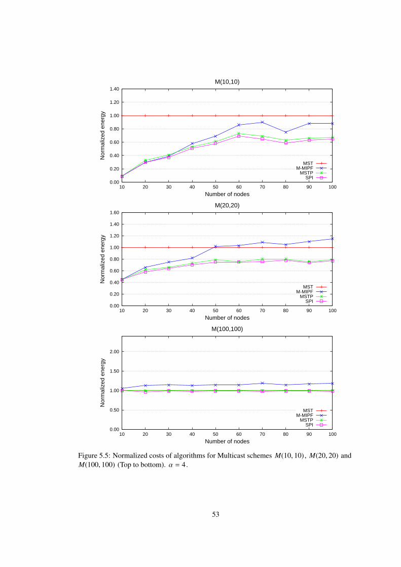
0.00

0.20

0.40

0.60

0.80

1.00

1.20

1.40

10 20 30 40 50 60 70 80 90 100

Nor

mal

ized

ene

rgy

Number of nodes

M(10,10)

MSTM-MIPF

MSTPSPI

0.00

0.20

0.40

0.60

0.80

1.00

1.20

1.40

1.60

10 20 30 40 50 60 70 80 90 100

Nor

mal

ized

ene

rgy

Number of nodes

M(20,20)

MSTM-MIPF

MSTPSPI

0.00

0.50

1.00

1.50

2.00

10 20 30 40 50 60 70 80 90 100

Nor

mal

ized

ene

rgy

Number of nodes

M(100,100)

MSTM-MIPF

MSTPSPI

Figure 5.5: Normalized costs of algorithms for Multicast schemes M(10, 10), M(20, 20) andM(100, 100) (Top to bottom). α = 4.

53

CHAPTER 6

GUI FOR ALGORITHM VISUALIZATION

In this chapter, we give detailed information about the graphical user interface, which is de-

veloped to run algorithms and visualize their behaviors. Figure 6.1 shows the main window

of the application. Main screen has two different parts. Left of the window is the free space

that is used to deploy network topologies. Right part contains the controls used to manage

network topology, create multicast schemes and specify algorithm type. Algorithm type and

multicast schemes are given as inputs to the system. Left panel is also used to visualize the

execution results of the algorithms. After the range assignment, range values are displayed on

the network topology.

Figure 6.1: Main Screen.

In order to deploy a wireless sensor network topology user enters the node number of the

54

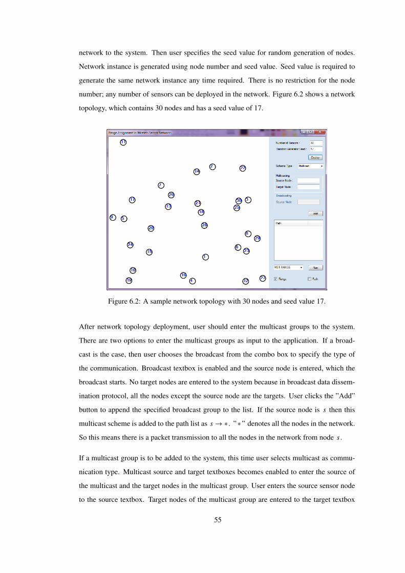
network to the system. Then user specifies the seed value for random generation of nodes.

Network instance is generated using node number and seed value. Seed value is required to

generate the same network instance any time required. There is no restriction for the node

number; any number of sensors can be deployed in the network. Figure 6.2 shows a network

topology, which contains 30 nodes and has a seed value of 17.

Figure 6.2: A sample network topology with 30 nodes and seed value 17.

After network topology deployment, user should enter the multicast groups to the system.

There are two options to enter the multicast groups as input to the application. If a broad-

cast is the case, then user chooses the broadcast from the combo box to specify the type of

the communication. Broadcast textbox is enabled and the source node is entered, which the

broadcast starts. No target nodes are entered to the system because in broadcast data dissem-

ination protocol, all the nodes except the source node are the targets. User clicks the ”Add”

button to append the specified broadcast group to the list. If the source node is s then this

multicast scheme is added to the path list as s→ ∗ . ”∗” denotes all the nodes in the network.

So this means there is a packet transmission to all the nodes in the network from node s .

If a multicast group is to be added to the system, this time user selects multicast as commu-

nication type. Multicast source and target textboxes becomes enabled to enter the source of

the multicast and the target nodes in the multicast group. User enters the source sensor node

to the source textbox. Target nodes of the multicast group are entered to the target textbox

55

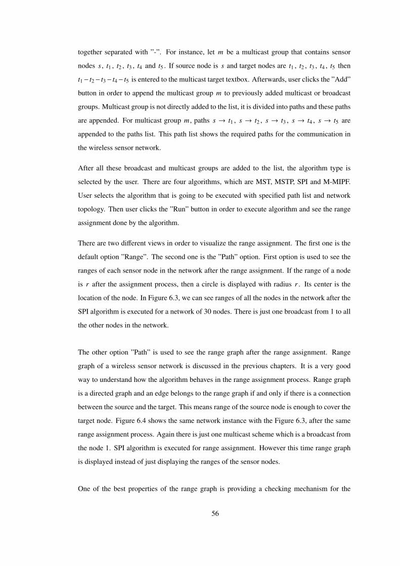
together separated with ”-”. For instance, let m be a multicast group that contains sensor

nodes s , t1 , t2 , t3 , t4 and t5 . If source node is s and target nodes are t1 , t2 , t3 , t4 , t5 then

t1− t2− t3− t4− t5 is entered to the multicast target textbox. Afterwards, user clicks the ”Add”

button in order to append the multicast group m to previously added multicast or broadcast

groups. Multicast group is not directly added to the list, it is divided into paths and these paths

are appended. For multicast group m , paths s → t1 , s → t2 , s → t3 , s → t4 , s → t5 are

appended to the paths list. This path list shows the required paths for the communication in

the wireless sensor network.

After all these broadcast and multicast groups are added to the list, the algorithm type is

selected by the user. There are four algorithms, which are MST, MSTP, SPI and M-MIPF.

User selects the algorithm that is going to be executed with specified path list and network

topology. Then user clicks the ”Run” button in order to execute algorithm and see the range

assignment done by the algorithm.

There are two different views in order to visualize the range assignment. The first one is the

default option ”Range”. The second one is the ”Path” option. First option is used to see the

ranges of each sensor node in the network after the range assignment. If the range of a node

is r after the assignment process, then a circle is displayed with radius r . Its center is the

location of the node. In Figure 6.3, we can see ranges of all the nodes in the network after the

SPI algorithm is executed for a network of 30 nodes. There is just one broadcast from 1 to all

the other nodes in the network.

The other option ”Path” is used to see the range graph after the range assignment. Range

graph of a wireless sensor network is discussed in the previous chapters. It is a very good

way to understand how the algorithm behaves in the range assignment process. Range graph

is a directed graph and an edge belongs to the range graph if and only if there is a connection

between the source and the target. This means range of the source node is enough to cover the

target node. Figure 6.4 shows the same network instance with the Figure 6.3, after the same

range assignment process. Again there is just one multicast scheme which is a broadcast from

the node 1. SPI algorithm is executed for range assignment. However this time range graph

is displayed instead of just displaying the ranges of the sensor nodes.

One of the best properties of the range graph is providing a checking mechanism for the

56

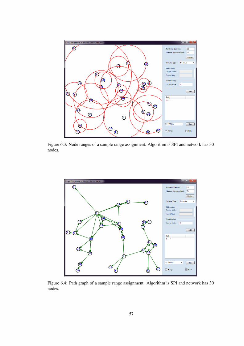
Figure 6.3: Node ranges of a sample range assignment. Algorithm is SPI and network has 30nodes.

Figure 6.4: Path graph of a sample range assignment. Algorithm is SPI and network has 30nodes.

57

assignment process after the algorithm is executed. Using the range graph, user can control if

all the paths in the list are satisfied with this assignment. For example, for nodes s and t , if

path s− > t is in the paths list, which means s is the source node and t is the target node and

there is a data transmission from node s to node t , then there must be a path between these

two nodes in the range graph. User can traverse and check for a path between nodes on the

range graph.

”Range” and ”Path” options can be used at the same time in the application. User checks both

of the checkboxes and both the circles denoting the ranges of the nodes and the range graph

of the network are displayed. Figure 6.5 shows this alternative.

Figure 6.5: Path graph and node ranges of a sample range assignment. Algorithm is SPI andnetwork has 30 nodes.

58

CHAPTER 7

CONCLUSION

In this thesis, we have defined the static range assignment problem and have proposed MST,

MSTP and SPI algorithms as efficient heuristics to solve this problem. MST algorithm is

developed as a baseline to other algorithms. It constructs a minimum spanning tree on the

network and makes the range assignment using this minimum spanning tree. MST algorithm

uses a naive approach and does not make a very effective assignment. A pruning procedure is

applied with the MSTP algorithm over the MST algorithm to get better results. SPI algorithm

is the third algorithm proposed, it is the most sophisticated one from these three algorithms.

It uses a shortest path based approach and advantage of wireless medium in its design.

After describing the SRA problem and propose these algorithms, we have defined the multiple

source multicasting in wireless sensor networks and have introduced the MEMSM problem

as a special case of SRA problem. MEMSM problem is a generalization of MEM problem.

It focuses on finding an energy efficient range assignment on sensor networks with multiple

multicast requests. We have presented the M-MIPF algorithm as a baseline to the MEMSM

problem. It modifies the well-known algorithm MIPF which is developed for MEM problem.

We have implemented a graphical user interface to run our algorithms and visualize their

behaviors. Using this application it is possible to construct network instances with any node

number. Furthermore, the multicast scheme and algorithm type can be specified as inputs to

the system. The radius assignment and the range graph of the network could be displayed with

this interface. We have executed the MST, MSTP, SPI and M-MIPF algorithms with different

network sizes and various multicast schemes for evaluation. We have calculated their energy

expenditures using a cost function.

In our evaluation we have used the normalized costs of algorithms according to the baseline

59

MST algorithm. We have generated different graphics for each multicast scheme. Evaluation

results show that the SPI algorithm performs better than other three algorithms for almost all

different network sizes and multicast schemes. MSTP and M-MIPF algorithms has a simi-

lar performance for small node numbers, however for bigger networks the MSTP algorithm

outperforms the M-MIPF algorithm. Therefore algorithms developed for MEMSM problem,

which are MSTP and SPI outperforms the algorithm M-MIPF, which is a modified version of

MIPF algorithm that solves the MEM problem.

A multiple source multicasting is a possible scenario for wireless sensor networks and as a

result of these experiments, we conclude that our algorithms MSTP and SPI are stable and

energy efficient solutions to MEMSM problem. However our most sophisticated algorithm is

SPI and it outperforms even the MSTP algorithm.

In our thesis we assume that all the nodes in the network use omni directional antennas. As a

future work, our algorithms can be modified considering that some of the nodes might have

directional antennas. Furthermore all of the algorithms are developed for the wireless sensor

networks, which have stationary sensor nodes. Their designs can be improved for handling

mobile sensor nodes in the network. In our cost calculations we consider only the energy

spent for communication between nodes, for more accurate results the processing costs of

nodes can also be taken into account.

60

REFERENCES

[1] I. F. Akyildiz, W. Su, Y. Sankarasubramaniam, and E. Cayirci. Wireless sensor net-works: a survey. Computer Networks, 38(4):393 – 422, 2002.

[2] E. Althaus, G. Calinescu, I. I. Mandoiu, S. Prasad, N. Tchervenski, and A. Zelikovsky.Power efficient range assignment for symmetric connectivity in static ad hoc wirelessnetworks. Wirel. Netw., 12(3):287–299, 2006.

[3] G. Anastasi, M. Conti, M. Di Francesco, and A. Passarella. Energy conservation inwireless sensor networks: A survey. Ad Hoc Networks, 7(3):537–568, 2009.

[4] M. Cagalj, J.P. Hubaux, and C. Enz. Minimum-energy broadcast in all-wireless net-works: NP-completeness and distribution issues. In Proceedings of the 8th annual in-ternational conference on Mobile computing and networking, pages 172–182. ACM,2002.

[5] J. Cartigny, D. Simplot, and I. Stojmenovic. Localized minimum-energy broadcastingin ad-hoc networks. In IEEE Societies INFOCOM 2003. Twenty-Second Annual JointConference of the IEEE Computer and Communications, pages 2210–2217, 2003.

[6] D. Chen and P.K. Varshney. QoS support in wireless sensor networks: A survey. InInternational Conference on Wireless Networks, pages 227–233, 2004.

[7] A.K. Das, R.J. Marks, M. El-Sharkawi, P. Arabshahi, and A. Gray. r-shrink: A heuristicfor improving minimum power broadcast trees in wireless networks. In IEEE GlobalTelecommunications Conference, 2003. GLOBECOM’03, volume 1, 2003.

[8] Arindam K. Das, Robert J. Marks, Mohamed El-sharkawi, Payman Arabshahi, and An-drew Gray. Minimum power broadcast trees for wireless networks: Integer program-ming formulations. In in Proc. IEEE Int. Symp. on Circuits and Systems, pages 245–248,2003.

[9] Edsger Wybe Dijkstra. A Note on Two Problems in Connection with Graphs. NumericalMathematics, 1:269–271, 1959.

[10] Christophe Diot, Walid Dabbous, and Jon Crowcroft. Multipoint communication: Asurvey of protocols, functions, and mechanisms. IEEE Journal on Selected Areas inCommunications, 15(3):277–290, 1997.

[11] S. Guo and O. Yang. A dynamic multicast tree reconstruction algorithm for minimum-energy multicasting in wireless ad hoc networks. In 2004 IEEE International Confer-ence on Performance, Computing, and Communications, pages 637–642, 2004.

[12] S. Guo and O.W. Yang. Minimum-energy multicast routing in static wireless ad hocnetworks. In 2004 IEEE 60th Vehicular Technology Conference, 2004. VTC2004-Fall,pages 3989–3993, 2004.

61

[13] Song Guo and Oliver W. W. Yang. Energy-aware multicasting in wireless ad hoc net-works: A survey and discussion. Comput. Commun., 30(9):2129–2148, 2007.

[14] F. Ingelrest et al. Localized broadcast incremental power protocol for wireless ad hocnetworks. Wireless Networks, 14(3):309–319, 2008.

[15] I. Kang, R. Poovendran, and WASHINGTON UNIV SEATTLE DEPT OF ELECTRI-CAL ENGINEERING. Broadcast with heterogeneous node capability. 2004.

[16] D. Li, Q. Liu, X. Hu, and X. Jia. Energy efficient multicast routing in ad hoc wirelessnetworks. Computer Communications, 30(18):3746–3756, 2007.

[17] N. Li, J.C. Hou, and L. Sha. Design and analysis of an MST-based topology controlalgorithm. IEEE Transactions on Wireless Communications, 4(3):1195, 2005.

[18] X.Y. Li. Approximate MST for UDG locally. Computing and Combinatorics, pages364–373, 2003.

[19] W. Liang. Constructing minimum-energy broadcast trees in wireless ad hoc networks.In Proceedings of the 3rd ACM international symposium on Mobile ad hoc networking& computing, page 122. ACM, 2002.

[20] F. Nait-Abdesselam, B. Bensaou, T. Soete, and K.L. Hung. O-MAC: An OrganizedEnergy-aware MAC Protocol for wireless sensor networks. In IEEE International Con-ference on Communications, 2007. ICC’07, pages 3648–3653, 2007.

[21] K. Obraczka and G. Tsuduk. Multicast routing issues in ad hoc networks. In IEEE 1998International Conference on Universal Personal Communications, 1998. ICUPC’98,volume 1, 1998.

[22] C.E. Perkins. Ad hoc networking. Addison-Wesley Professional, 2008.

[23] R.C. Prim. Shortest connection networks and some generalizations. Bell system techni-cal journal, 36(6):1389–1401, 1957.

[24] P.M. Ruiz and A.F. Gomez-Skarmeta. Reducing data-overhead of mesh-based ad hocmulticast routing protocols by Steiner tree meshes. 2004.

[25] Loren Schwiebert, Sandeep K.S. Gupta, and Jennifer Weinmann. Research challengesin wireless networks of biomedical sensors. In MobiCom ’01: Proceedings of the 7thannual international conference on Mobile computing and networking, pages 151–165,New York, NY, USA, 2001. ACM.

[26] P. J. Wan, G. Calinescu, X. Y. Li, and O. Frieder. Minimum-energy broadcasting instatic ad hoc wireless networks. Wirel. Netw., 8(6):607–617, 2002.

[27] P.J. Wan, G. Calinescu, and C.W. Yi. Minimum-power multicast routing in static adhoc wireless networks. IEEE/ACM Transactions on Networking (TON), 12(3):507–514,2004.

[28] B. Wang and S.K.S. Gupta. S-REMiT: a distributed algorithm for source-based energyefficient multicasting in wireless ad hoc networks. In IEEE GLOBECOM, volume 3.Citeseer, 2003.

62

[29] Jeffrey E. Wieselthier, Gam D. Nguyen, and Anthony Ephremides. Energy-efficientbroadcast and multicast trees in wireless networks. Mob. Netw. Appl., 7(6):481–492,2002.

[30] J. Yick, B. Mukherjee, and D. Ghosal. Wireless sensor network survey. ComputerNetworks, 52(12):2292–2330, 2008.

[31] J. Zhu, S. Chen, B. Bensaou, and K.L. Hung. Tradeoff between lifetime and rate allo-cation in wireless sensor networks: A cross layer approach. In IEEE INFOCOM 2007.26th IEEE International Conference on Computer Communications, pages 267–275,2007.

63