Static and Dynamic Aspects of Voltage-Power relationships

IOSR Journal of Electrical and Electronics Engineering (IOSR-JEEE)

e-ISSN: 2278-1676,p-ISSN: 2320-3331, Volume 9, Issue 4 Ver. I (Jul – Aug. 2014), PP 01-12

www.iosrjournals.org

www.iosrjournals.org 1 | Page

Static and Dynamic Aspects of Voltage-Power relationships in

Electric Power Systems

Stephen R. Fernandes1

1Department of Electrical Engineering, Petrofac Engineering India Ltd., Mumbai, India; formerly a Ph.D

candidate at the University of Illinois at Urbana-Champaign, Illinois, USA.

Abstract: This paper investigates various aspects of voltage-power relationships in power systems. Conditions

for feasible generating points are analytically derived for a simple power system with a detailed generator

model. The set of Hopf Bifurcation points for the sample system are visualized on the feasible operating surface.

The effect of damping on the onset of bifurcations in the system is briefly investigated. The role of different

generator models in isolating bifurcations and subsidiary phenomena in a multi-machine system are also

presented. The effect of nonlinear indices of voltage dependent load models on system bifurcations is dealt with

as also the effect of AVR gains.

Keywords - Steady-state Stability, bifurcations, critical eigenvalues, P-V curves.

I. INTRODUCTION Power Systems are large complex dynamical systems. The nature of voltage-power relationships at any

bus within such systems likewise varies in a complex manner depending on where and how the system is

stressed, where the generating nodes are, network parameters and a host of other factors. Deriving explicit

expressions for such complex voltage-power behaviour at any bus in a stressed system is too intricate. However,

power system researchers have visualized such relationships using power-voltage (PV) curves constructed using

detailed power system models.

Power voltage curves have as such long been visualized and used in the analysis for various

phenomena in stressed power systems including structural stability, voltage instability, bifurcations etc. ([2]-

[5]). The dynamic aspects of such voltage power characteristics have also been studied in detail ([2]-[4]).

Dynamic models of power systems coupled with P-V curves present the researcher with tools to analyze both

static and dynamic aspects of power systems. However, it is interesting to note that the amount of detail used in

constructing dynamic system models is crucial in highlighting phenomena which usually cannot be visualized in

reduced order models. Adequate load modeling at different buses also play an important role in predicting the

occurrence of such dynamic phenomena.

This paper discusses the static and dynamic aspects of voltage-power characteristics in two sample

power systems. The onset of dynamic phenomena such as Hopf bifurcations is visualized using voltage-power

characteristics at a load bus. The effect of different detailed models on defining the onset of such phenomena is

investigated. The nature of different static load models, their power-voltage characteristics, their sensitivities

with respect to voltage variations and their effect on the occurrence of Hopf bifurcations is also investigated.

The effect of AVR gain Ka on the onset of such dynamic phenomena is also briefly dealt with.

II. SYSTEM DYNAMIC MODEL

A simple power system consisting of a single generator synchronized on an infinite bus through a

lumped transmission line, as shown in Fig. 1, is analyzed. The generator is modeled by a two axis machine

model with IEEE Type 1 exciter and a simplified turbine-governor model. The saturation effects in the generator

along with both stator and network transients are neglected. The synchronous machine equations are:

Sdt

d

(2.1)

M

D

M

IIXE

M

IIXE

M

T

dt

d SdqqdqddqM

(2.2)

do

fd

do

ddd

do

qq

T

E

T

IXX

T

E

dt

Ed

(2.3)

qo

qqq

qo

dd

T

XXI

T

E

dt

Ed

(2.4)

Static and Dynamic Aspects of Voltage-Power relationships in Electric Power Systems


The IEEE Type I exciter dynamics are given by:

E

Rfd

E

fdEEfd

T

VE

T

ESK

dt

dE

(2.5)

VV

T

KE

TT

KKR

T

K

T

V

dt

dVref

A

Afd

FA

FAF

A

A

A

RR (2.6)

fd

F

F

F

FF ET

K

T

R

dt

dR

2 (2.7)

where refV is a set point and V is the magnitude of the generator terminal voltage. The simplified turbine and

governor model is given by:

SV

CH

HPCH

CH

HP

RHRH

MM PT

KP

T

K

TT

T

dt

dT

1 (2.8)

CH

SV

CH

CHCH

T

P

T

P

dt

dP (2.9)

1

1

SSVdSV

C

SV

SVSV

TRT

P

T

P

dt

dP

(2.10)

In the above model, )( fdex EB

exfdE AES models the saturation in the exciter and M = 2H/ S , S =

120 rads/sec. The following limit constraints also apply to the model

maxminRRR VVV and max0 SVSv PP (2.11)

The stator algebraic equations to be satisfied are:

0sin qqdSd IXIRVE (2.12)

0cos ddqSq IXIRVE (2.13)

For the single machine infinite bus case the network equations to be satisfied are :

0sinsin VVIXIR qede (2.14)

0coscos VVIRIX qede (2.15)

The differentio-algebraic model illustrated above can be symbolically represented as :

pYXfX ,, (2.16)

pYXg ,,0 (2.17)

where X is the vector containing all differential states, Y is the vector containing all algebraic states and p is the

vector of all system parameters. The above model can be linearized about an equilibrium point. The symbolic

representation of the perturbation model has the form:



pEYBXAX (2.18)

pFYDXC 0 (2.19)

where

p

gF

Y

gD

X

gC

p

fE

Y

fB

X

fA

,,

,,

and YX , denote perturbation in the differential and algebraic states, p denotes perturbation in system

parameters. Eliminating Y from equations (2.18) and (2.19) we have the following representation:

pGXAX SYS (2.20)

where FBDEGCBDAASYS11 , . The eigenvalues to be observed are the eigenvalues of the

SYSA matrix.

III. FEASIBLE GENERATING SET The network algebraic equations (2.14) and (2.15) of the single machine infinite bus system model

outlined in section 2 are derived from the following equation satisfying Kirchoff’s voltage law in the network:

02 jee

j

qdj VjXRjIIV

(3.1)

The complex generated power at the generator bus is given by:

2

j

qdj

GG jIIVjQP (3.2)

Using (3.2) we can eliminate the currents qd II , from (3.1) which then can be written as:

0jeej

GGj VjXRV

jQPV

(3.3)

or 02 jjeeGG VVjXRjQPV

(3.4)

Separating (3.4) into real and imaginary components and taking 1V p.u we have:

0cos2 aVV (3.5)

0sin bV (3.6)

where eGeGeGeG RQXPbXQRPa , . Eliminating from (3.5) and (3.6) we have the following

equation which can be solved for V

0222 abVV (3.7)

Multiplying the two equations corresponding to each of the two different signs in (3.7) we have:

012 2224 baVaV (3.8)

Two of the four solutions of (3.8) will correspond to two solutions of each of the two equations forming it.

Substituting 2Vq in (3.8) we have:

012 222 baqaq (3.9)

which has two roots

2

41212 222

2,1

baaaq

(3.10)



The two roots in (3.10) can be (a) both real and 0 or both real and 0 or (b) both imaginary with real parts

the same, depending on the term inside the square root being (i) 0 or (ii) < 0 respectively. When the two

solutions for q given by (3.10) are both real and < 0 or both imaginary then the four solutions for V in (3.8) are

guaranteed to be all imaginary leading to a loss of a feasible solution. Both solutions for q in (3.10) are negative

when

012 a or 21a (3.11)

Both solutions of q in (3.10) are imaginary when

0412 222 baa or 0144 2 ab

41 ab (3.12)

Consider again (3.7). The Jacobian of the L.H.S of (3.7) yields

22

12

bV

VJ (3.13)

1J fails to exist when V=0 which is a trivial solution or when



4101

2 2

22

bV

bV

(3.14)

The critical value of generator terminal voltage can thus be derived by substituting the critical value of b from

(3.12) into (3.14) which gives:

2141 22 abV CC (3.15)

From (3.11),(3.12) and (3.15) the set of all feasible generating points for the single machine infinite bus system

can be constructed as shown in Fig. 2b for a lossless line. The 3-dimensional feasible operating surface is a

conglomeration of all PG vs V curves of the form shown in Fig. 2a (for QG = 0.5 p.u), for all QG within the

desirable operating range. The locus of all operating points (where loss of existence of a feasible solution

occurs) can be found by joining the tip of all PG vs V curves for different QG in the desired range.

IV. BIFURCATION ANALYSIS For the system (2.16)-(2.17) with perturbation model given by (2.20), conditions for Hopf bifurcation

to occur are (a) a simple pair of imaginary eigenvalues of ASYS matrix cross the imaginary axis while the other

(n-2) eigenvalues are all in the left half plane and

(b) 0Re

jCj pp

jj

pdp

d (4.1)

that is, the rate of change of the real part of the critical pair of eigenvalues with variation of the jth parameter

jp , is nonzero at the point where the critical parameter jCj pp . In the feasible generating space shown in

Fig. 2b, the set of Hopf bifurcating points are isolated using the above criteria and the results shown in Fig. 2b.

The Hopf Bifurcating locus is plotted only for the upper part of the feasible operating surface that is only when

the critical eigenvalues move over from the left half to the right half of the complex plane. Increased damping

D, in equation (2.2), in the system causes the Hopf bifurcation locus to shift lower down the feasible operating

surface till for some value of damping the locus vanishes and the upper part of the feasible operating surface

ceases to have Hopf Bifurcation points beyond that critical damping. A critical value exists too when damping D

becomes negative in the model. To verify that the above linearized analysis is actually coherent with nonlinear

time domain simulation, three different feasible operating points in the feasible operating surface were chosen as

shown in Table 1.

The system was perturbed from these operating points and the nonlinear model was simulated using the

Simultaneous Implicit Trapezoidal Method with a constant time step of 0.005 sec. The results for each case are

as shown in Fig. 3. The system is stable for case (a), exhibits periodic cycles for case (b) which is the Hopf

bifurcation point under study and is constrained to exhibit supercritical bifurcation like phenomena for case(c)

depicting a realistic scenario.

V. MULTIMACHINE SYSTEMS The system model for a multimachine system is represented by a set of machine models each of the

form (2.1)-(2.11), along with the associated stator algebraic equations of the form (2.12)-(2.13) with parameters

in the above equations corresponding to each machine in the system. The set of network equations derived by

applying Kirchoff’s voltage laws to the system network are: (assuming an n bus system with m generators

synchronized on the first m network buses)

0coscossin1

n

k

ikkiikkiiLiiiqiiid YVVVPVIVIiii

(5.1)

0sinsincos1

n

k

ikkiikkiiLiiiqiiid YVVVQVIVIiii

i = 1, ......., m (5.2)



0cos1

n

k

ikkiikkiiL YVVVPi

(5.3)

0sin1

n

k

ikkiikkiiL YVVVQi

i = m+1, ....., n (5.4)

where PLi (Vi) , QLi(Vi) denote voltage dependent exponential load models at the ith bus.

TABLE 1

Case GG jQP Critical Eigenvalue Pair

(a) 1.14 + j 0.2 - 0.2028 j 4.7868 in L.H.P

(b) 1.14637 + j 0.2 0.0000 j 4.4518 at Hopf Bif.

(c) 1.15 + j 0.2 + 0.1523 j 4.3125 in R.H.P

The three machine nine bus Western System Coordinating Council (WSCC) system shown in Fig. 4 with model

parameters as given in [6] is chosen for analysis in this section. Four different generator models are used to

study the role of bifurcations in this system. The generator models chosen are:

(a) Model-A: Two-axis model with IEEE Type I exciter; same as outlined in section 2.

(b) Model-B: Flux decay model with fast exciter. The damper winding constants in model (a) are assumed to

be very small and are set to zero which in essence means that an integral manifold exists for these states.

Equation (2.4) can then be written as:

qqqd IXXE 0 (5.5)

We use equation (5.5) to eliminate dE from equations (2.4) and (2.12). The exciter is modeled

by one dynamic equation:

VVT

K

T

E

dt

dEref

A

A

A

fdfd (5.6)

(c) Model C: Two-axis model with fast exciter. The model is essentially the same as in (a) except that the

single exciter equation (5.6) replaces the set of three equations representing the IEEE Type I exciter.

(d) Model D: Flux decay model with IEEE Type I exciter. The generator model is the same as in case (b) but

the exciter is IEEE Type I with three dynamic equations, (2.5)-(2.7). For convenience, the turbine-governor

dynamics are not modeled in any of the above. The zero eigenvalue inherent in such models is removed by

introducing relative rotor angles.



VI. STATIC LOAD MODELS Loads are a part of every power system and their characteristics do affect the dynamic behaviour of

such systems. So, when power networks are modeled for analysis effective load modeling becomes an essential

step in the process. Past literature ([7]-[12]) abounds in different modeling aspects of static and dynamic load

models.

Effective load models as such, should be realistic, simple and strike a proper balance among the

different load mixes existing in the actual system. Such load mix composition modeling requires reliable

estimation. Since, there is always an element of uncertainty in such estimation, prevalent load models are

inherently conservative by design. In this analysis presented here we stick to the generic load models which

have been presented in literature, more precisely we consider only voltage dependent exponential load models

of the form:

iii LLL jQPS at the ith bus where

i

i

ii

i

i

ii

nq

iL

np

iL

V

VQQ

V

VPP

00

00 , (6.1)

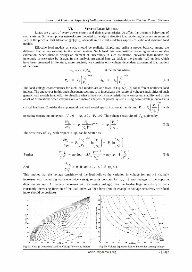
The load-voltage characteristics for such load models are as shown in Fig. 5(a)-(b) for different nonlinear load

indices. The endeavour in this and subsequent sections is to investigate the nature of voltage sensitivities of such

generic load models in an effort to visualize what effects such characteristics have on system stability and on the

onset of bifurcations when carrying out a dynamic analysis of power systems using power-voltage curves at a

critical load bus. Consider the exponential real load model approximation at the ith bus:

i

i

ii

np

iL

V

VPP

00 with

operating constraints (relaxed) : 0,0,0 0 i

PnpV i . The voltage sensitivity of iLP is given by:

i

L

inp

npii

L

V

PnpV

V

Pnp

V

Pii

i

i

ii 1

0

0 (6.2)

The sensitivity of iLP with respect to inp can be written as:

i

i

i

i

i

i

i

V

VP

V

V

V

VP

np

Pi

Li

np

i

i

L

0000 lnln

Further

2

0

2

02

2

11.

i

iiinp

npi

ii

i

L

V

Pnpnp

V

VPnpnp

V

P

i

i

i

i

i (6.4)

And 02

2

i

L

V

Pi if 0,1 inp if 1inp

This implies that the voltage sensitivity of the load follows the variation in voltage for 1inp (namely

increases with increasing voltage or vice versa), remains constant for 1inp and changes in the opposite

direction for 1inp (namely decreases with increasing voltage). For the load-voltage sensitivity to be a

constantly increasing function of the load index we then have (rate of change of voltage sensitivity with load

index should be positive):

Fig. 5a. Voltage Dependent Load Vs Voltage for varying Indices Fig. 5b Voltage dependent load vs Indices for varying Voltage



Fig. 5c. Voltage Dependent Load Sensitivity vs Voltage for Fig.5d. Voltage Dependent Load Sensitivity (w.r.t Index) vs Indices for

varying Indices varying Voltages

Fig. 5e. Voltage dependent Load Sensitivity (w.r.t voltage) vs Fig.5f. Voltage Dependent Load Sensitivity vs Voltage for varying Indices for varying Voltage exponents

i

i

i

ii

i

i

ii

V

VV

V

PnpV

V

P

Vnp

Pinp

inpinp

inpii

L

0

101

0

02

ln.

0ln10

1

0

0

i

i

i

i

i

V

VnpV

V

Pi

inp

inp (6.5)

or i

iii

npV

V

V

Vnp

ii

1ln0ln1

00

or

inp

iVVi

1

0

(6.6)

The load-voltage sensitivity is a constantly increasing function for V > 0 if 0inp , V > 0.3679 0V for

1inp and 06065.0 VV if .2inp I other words a positive change in voltage index inp (due to a change in

the aggregation of loads) brings about a positive change in the voltage sensitivity of load approximated by the

exponential load model. Figs. 5(c)-(f) show the behaviour of these sensitivities for upPupVi

.1,.1 00

(normalized load constants).

VII. ROLE OF GENERATOR MODELS IN ISOLATING

BIFURCATION POINTS The real power at load bus 5 in the WSCC system is chosen as the critical parameter for the system

represented by each of the models (a)-(d) in section 5. The bifurcation analysis yields the results as shown in

Table 2 for constant power case 0 ii nqnp . The modal behaviour of each of these models is as shown in

Fig. 6(a)-(b). JLF denotes the Jacobian of the network equations with respect to the network variables and JAE,



the Jacobian of the stator and network equations with respect to all the algebraic variables: network variables

and the stator currents. It is seen that in model (b) and (c) with fast exciters, another pair of eigenvalues joins

the critical pair in the left half plane. This second pair is associated with the rotor variables of the second

generator 22 , . They follow the movement of the critical pair and move back into the left half plane after

the critical pair have split along the real axis, point B, in Fig. 6(b). The movement of both these pairs are

captured in Table 3 as the real power at bus 5 is increased.

TABLE 2.1 Modal Behaviour of Model (a) for different Loads Load at Bus 5 Sign(det JLF) Sign(det JAE) Critical Eigenvalue(s) Associated States

4.3 + + -0.1433 j2.0188 11 & fq RE

4.4 + + 0.0057 j2.2434 11 & fq RE

4.5 + + 0.3400 j2.5538 11 & fq RE

4.6 + + 1.1350 j2.8016 11 & fq RE

4.7 + + 2.5961 j2.2768 11 & fq RE

4.8 + + 9.2464, 1.8176 1122 &,& fq RE

4.9 + - 1.0542 11 & fq RE

5.0 + - 0.6298 11 & fq RE

5.1 + - 0.2463 11 & fq RE

5.15 + - -0.6832 11 & fq RE

5.2 Load Flow does not converge

TABLE 2.2 Modal Behaviour of Model (b) for different loads Load at Bus 5 Sign(det JLF) Sign(det JAE) Critical Eigenvalue(s) Associated States

4.4 + + -0.0957 j0.1407 22 &

4.5 + + 0.0308 j10.0034 22 &

4.6 + + 0.3802 j9.9008 22 &

4.7 + + 0.9344 j10.1111 22 &

4.8 + + 1.3907 j11.1963 22 &

4.9 + - 24.4174, 0.1104 j11.3605 11 & fdq EE , 22 &

5.0 + - 6.0978 11 & fdq EE

5.1 + - 2.5680 11 & fdq EE

5.15 + - 0.5417 11 & fdq EE


TABLE 2.3 Modal Behaviour of Model (c) for different Loads Load at Bus 5 Sign(det JLF) Sign(det JAE) Critical Eigenvalue(s) Associated States

4.2 + + -0.0048 j7.4848 22 &

4.3 + + 0.2522 j7.4248 22 &

4.4 + + 0.5333 j7.4024 22 &

4.5 + + 0.8574 j7.4233 22 &

4.6 + + 1.2592 j7.5151 22 &

4.7 + + 1.8164 j7.7697 22 &

4.8 + + 2.7800 j8.6826 22 &

4.9 + - 12.2699, 0.4398 j10.0051 11 & fdq EE , 22 &

5.0 + - 4.1693,0.1100 j9.3208 11 & fdq EE , 22 &

5.1 + - 1.6687 11 & fdq EE

5.15 + - 0.0369 21 &




TABLE 2.4 Modal Behaviour of Model (d) for different loads Load at Bus 5 Sign(det JLF) Sign(det JAE) Critical Eigenvalue(s) Associated States

4.4 + + -0.2388 j1.6434 11 & fq RE

4.5 + + -0.1997 j1.7778 11 & fq RE

4.6 + + -0.1265 j1.9985 11 & fq RE

4.7 + + 0.0614 j2.4531 11 & fq RE

4.8 + + 1.7612 j3.9016 11 & fq RE

4.9 + - 1.8483 11 & fq RE

5.0 + - 0.9059 11 & fq RE

5.1 + - 0.3726 11 & fq RE

5.15 + - -0.0424 211 &, fq RE


TABLE 3. Modal Behaviour of Model (b) for increasing load at bus 5 for Ka=50 Load at Bus 5 Sign(det JLF) Sign(det JAE) Critical Eigenvalue(s) Associated States

4.80 + + 1.3907 j11.1963 22,

4.82 + + 0.0443 j15.5037

1.1546 j11.6623

22,

4.84 + + 0.5983 j11.7688

1.9965 j15.7308

22,

4.86 + + 0.3174 j11.5990

3.5964 j17.9186

22,

4.88 + + 0.1862 j11.4621

8.8996 j26.1149

22,

11, fdq EE 4.90 + - 24.4175, 0.1105 j11.3605 11, fdq EE

4.92 + - 14.0688, 0.0611 j11.2824 11, fdq EE

4.94 + - 10.5866, 0.0265 j11.2200 11, fdq EE

4.96 + - 8.5713, 0.0010 j11.1686 11, fdq EE

4.98 + - 7.1711 11, fdq EE

5.00 + - 6.0978 11, fdq EE

5.02 + - 5.2207 11, fdq EE

5.04 + - 4.4687 11, fdq EE

5.06 + - 3.7973 11, fdq EE

5.08 + - 3.1738 11, fdq EE



VIII. EFFECT OF NONLINEARITY OF LOAD MODELS ON

BIFURCATIONS Table 4 depicts the effect of nonlinear load indices on Hopf bifurcation points for different generator

models chosen for each value of critical loading parameter, the real power at bus 5. The AVR gain Ka is chosen

as 25. It is seen that the flux decay model (neglecting damper winding dynamics) essentially makes the system

more stable and Hopf bifurcations occur at a later stage. The type of exciter model used also has some influence

on the bifurcation point; model (c), which is a flux decay model coupled with a fast exciter, undergoes Hopf

Bifurcations at a much later stage than the other models.

TABLE 4 Effect of Nonlinearity of Loads on Bifurcation Points of Different Models Load (in p.u) at Bus 5 at corresponding Hopf Bifurcation Point

Load Index Model (a) Model (b) Model (c) Model (d)

0.0 4.4 4.6 4.4 4.7

0.1 4.55 4.7 4.5 4.8

0.2 4.65 4.8 4.6 4.95

0.5 5.05 5.1 4.95 5.15

0.6 - - 5.05 -

0.7 - - 5.10 -

0.8 - - 5.15 -

0.9 - - - -

IX. EFFECT OF EXCITER GAIN

The exciter gain Ka (assumed same for all machines in the system) also has some influence on the

onset of Hopf bifurcations essentially prolonging their occurrence for higher values as shown in Fig. 7 for model

(a).

X. CONCLUSIONS Power voltage relationships in power systems were investigated. The effect of different generator

models in defining stability of multimachine systems were dealt upon using power voltage relationships at a

critical load bus. The effect of nonlinear voltage dependent load characteristics on system stability and the onset

of bifurcations was shown as also the effect of AVR gain. Further work is needed to fully understand power

voltage relationships and the occurrence of dynamic phenomena apart from simple Hopf Bifurcations, for

example, period doubling bifurcations and chaos, in large power systems.



ACKNOWLEDGEMENTS The author would like to thank Mr. Anil V Borkar, Girish Kulkarni, Simmon Sakia, Tapendra Guha,

Ghulam Jilani, Vinod Keswani, Parag Soni and Amit Nadkarni of Petrofac for their unconditional support

during the development of this paper.

REFERENCES [1] J. Guckenheimer and P.Holmes, Nonlinear Oscillations, Dynamical Systems and Bifurcations of vector fields,’ Applied mathematical

Sciences 42, Springer-Verlag, 1983.

[2] V. Ajjarapu and B.Lee, ‘Bifurcation theory and its application to nonlinear dynamical phenomena in an electric power system,’ IEEE Transactions on Power Systems, vol 7, No.1, February 1992, pp 424-431.

[3] P.W.Sauer, B.C. Lesieutre and M.A.Pai, ‘ Dynamic vs Static aspects of voltage problems,’ Bulk Power System Voltage Phenomena, voltage stability and security, International Workshop, Deep Creek Lake, Maryland, Aug 4-7, 1991.

[4] C.Rajagopalan, B.Lesieutre, P.W.Sauer and M.A.Pai, ‘Dynamic Aspects of Voltage/Power characteristics,’ IEEE Transactions on

Power Systems, vol 7, No. 3, August 1992, pp 990-1000. [5] M.A.Pai, P.W.Sauer, B.C. Lesieutre and A.Adapa, ‘Structural Stability in Power Systems- Effect of Load Models,’ IEEE

Transactions on Power Systems, Vol. 10, No. 2, May 1995, pp 609-615.

[6] EPRI Final Report, ‘Power System Dynamic Analysis,’ Phase I, EL 484, Project 670-1, July 1977.

[7] EPRI Final Report EL-850, Project 849-1, ‘Determining Load Characteristics for Transient Performance,’ Vol 1-4, prepared by

General Electric Company, Schenectady, New York, March 1981.

[8] EPRI Final Report EL-5003, Project 849-7, ‘Load Modeling for Power flow and Transient Stability computer services,’ Vol 1 and 2, prepared by General Electric Company, Schenectady, New York, Jan 1987.

[9] B.C. Lesieutre, P.W. Sauer and M.A.Pai, ‘Sufficient conditions on static load models for network solvability,’ Proceedings of the

Twenty-Fourth Annual North American Power Symposium, Reno, NV, Oct 5-6, 1992, pp 262-271. [10] C.Concordia and S.Ihara, ‘Load representation in power system stability studies,’ IEEE Trans. On PAS, vol-101, No 4, April 1982,

pp 969-977.

[11] IEEE Task Force on load representation for dynamic performance, ‘Load representation for dynamic performance analysis,’ IEEE Trans. On Power Systems, PWRS-8, No.2, May 1993, pp 472-481.

[12] IEEE Task force on load representation for Dynamic performance, ‘Standard Load Models for Power Flow and Dynamic

Performance Simulation,’ IEEE Trans. On Power Systems, vol-10, No 3, Aug 1995, pp 1302-1313.

[13] S.R. Fernandes, P.W Sauer and M.A. Pai, ‘Quantification of Parameter Importance in Power Systems Steady State Stability

Analysis,’ Proceedings of the 28th North American Power Symposium, Massachussetts Institute of Technology, Cambridge, MA, USA, November 10-12, 1996, pp. 133-138.

[14] S.R. Fernandes, ‘Generalized Extension of AESOPS and PEALS Algorithms for Sensitivity Analysis,’ Journal of the Institution of

Engineers, Singapore, vol 45, Issue 1, 2005, pp. 14-37.

APPENDIX A

SR dX qX dX qX 0dT

0.00185p.u 1.942p.u 1.921p.u 0.330p.u 0.507p.u 5.330p.u

0qT H D eX AK AT

0.593 s 2.8323 s 0.0 p.u 0.5 50 0.02

EK ET FK FT exA exB

1.0 0.78 0.01 1.2 0.397 0.09

maxrV minrV RHT HPK CHT SVT

9.9 -8.9 10.0 0.26 0.5 0.2

Documents

Static and Dynamic Aspects of Voltage-Power relationships