Static Aeroelastic Analysis with an Inviscid Cartesian … · Static Aeroelastic Analysis with an Inviscid Cartesian Method David L. Rodriguez* Science & Technology Corp., Moffett

Static Aeroelastic Analysis with an Inviscid Cartesian Method

David L. Rodriguez*

Science & Technology Corp., Moffett Field, CA 94305Michael J. Aftosmis†

NASA Ames Research Center, Moffett Field, CA 94305

Marian Nemec‡

Science & Technology Corp., Moffett Field, CA 94305Stephen C. Smith§

Zee Aero, Mountain View, CA 94043

An embedded-boundary, Cartesian-mesh flow solver is coupled with a three degree-of-freedom structural model to perform static, aeroelastic analysis of complex aircraft geome-tries. The approach solves a nonlinear, aerostructural system of equations using a loosely-coupled strategy. An open-source, 3-D discrete-geometry engine is utilized to deform a trian-gulated surface geometry according to the shape predicted by the structural model under the computed aerodynamic loads. The deformation scheme is capable of modeling large deflec-tions and is applicable to the design of modern, very-flexible transport wings. The coupling interface is modular so that aerodynamic or structural analysis methods can be easily swapped or enhanced. After verifying the structural model with comparisons to Euler beam theory, two applications of the analysis method are presented as validation. The first is a relatively stiff, transport wing model which was a subject of a recent workshop on aeroelas-ticity. The second is a very flexible model recently tested in a low speed wind tunnel. Both cases show that the aeroelastic analysis method produces results in excellent agreement with experimental data.

I. IntroductionIn contrast to the relatively rigid aluminum wings of the past seven decades, modern composite wings are sig-

nificantly more flexible. For instance, even at cruise, the wing on the Boeing 787 Dreamliner will nominally deflect ten feet (10% of the semispan) as depicted in Figure 1. The weight savings realized by composite construction com-bined with active load alleviation and other modern flight controls point toward a future of ever more flexible trans-port aircraft. Both the D8 “Double Bubble”1 (Figure 2) and truss-braced-winged “SUGAR”2 (Figure 3) concept air-

1American Institute of Aeronautics and Astronautics

* Senior Research Scientist, Applied Modeling and Simulation Branch, MS 258-5; [email protected]. Senior AIAA Member.† Aerospace Engineer, Applied Modeling and Simulation Branch, MS 258-5; [email protected]. Associate Fellow AIAA.‡ Senior Research Scientist, Applied Modeling and Simulation Branch, MS 258-5; [email protected]. Senior AIAA Member.§ Senior Aerodynamic Designer, Zee Aero. Associate Fellow AIAA.

Figure 1. Boeing 787 at cruise (courtesy of Boeing). Figure 2. The D8 “Double-Bubble” concept.

Dow

nloa

ded

by M

icha

el A

ftosm

is on

Janu

ary

13, 2

014

| http

://ar

c.ai

aa.o

rg |

DO

I: 10

.251

4/6.

2014

-083

6

55th AIAA/ASMe/ASCE/AHS/SC Structures, Structural Dynamics, and Materials Conference 13-17 January 2014, National Harbor, Maryland

AIAA 2014-0836

mailto:[email protected]






craft are designed around highly-flexible, high aspect-ratio, composite wings. Beyond these designs, future concepts will actively exploit wing flexibility through in-flight morphing to significantly improve performance allowing for even lighter construction. For example, the Variable Camber Continuous Trailing Edge Flap3 (VCCTEF) concept depicted in Figure 4 will be able to dynamically tailor the spanwise lift distribution to im-prove aerodynamic performance throughout an aircraft’s mission profile. Such concepts make accurate static and dynamic aeroelastic predictions more critical than ever. Traditional methods that assume small deflections and linear aerodynamics are no longer valid for these air-craft, and thus more advanced tools must be deployed early in the design cycle.

In the past few decades, aeroelastic analysis has been performed using a variety of approaches. Tradition-ally, linear aerodynamics methods (such as the Doublet Lattice Method4) have been closely coupled with finite element structural solvers (such as NASTRAN5) to cre-ate aerostructual analysis methods. Similarly, Drela6 combined linear lifting-line and nonlinear beam theories to create a fully-coupled analysis scheme that is solved by a global Newton method. While these schemes are often valuable for designing structurally stiff aircraft, linear aerodynamics is not sufficiently accurate for de-signing highly flexible aircraft. To employ higher-fidelity analysis methods, especially those with disparate solution schemes, a monolithic approach to solving the aerostructural problem is not always ideal. In 1992, Gu-ruswamy7 argued that monolithic static-aeroelastic solv-ers of the time were very computationally inefficient. Also, the ability to use variable-fidelity analysis methods without the need to completely rewrite an existing analy-sis tool to include cross-discipline terms is a very attrac-tive feature. Hence, a more loosely-coupled approach to solving the aeroelastic equations is often preferred.

Many loosely-coupled aeroelastic solvers have been developed in the past. In the late 1970’s, Chipman et. al.8 developed an iterative scheme that combined a transonic small disturbance solver with a slender beam structural model. Whitlow and Bennett9 loosely coupled a full po-tential flow solver with a finite element structural model that was appropriate for both high and low aspect-ratio wings. However, the method was only applicable to small deflections. Tatum and Giles10 built a similar and very modular tool for analyzing complete fighter aircraft with a full potential flow solver and an equivalent plate model instead of a finite element method. Guruswamy7 successfully coupled Euler and Navier-Stokes solvers with finite element methods based purely on simple beam elements. Martins11 solved a high-fidelity aerostructural model using a loosely-coupled approach with a geometry engine as the primary interface. That method also allowed for adjoint-based design optimization.

This paper presents the first steps in the development of an inexpensive, static-aeroelastic analysis capability that leverages the versatility of an inviscid Cartesian-mesh solver and a mid-fidelity structural analysis model that idealizes the wing structure as a series of tapered beams. While similar to previously analysis methods,9-11 the pre-sented loosely-coupled analysis procedure is also designed to handle discrete geometry whether it is a legacy surface mesh or derived from modern computer-aided design software. One major advantage of utilizing a Cartesian-mesh flow solver is that volume mesh perturbation schemes used by many tools in the past7,9-11 are not necessary. No mat-ter how much a wing deforms, a quality volume mesh is generated on-the-fly. High-fidelity Cartesian Euler solvers are also computationally efficient enough to be used even at the conceptual level of design. In the future, this capa-


Figure 4. Representation of an aircraft using the Variable Camber Continuous Trailing Edge Flap concept.

Figure 3. The SUGAR truss-braced wing concept.

Dow

nloa

ded

by M

icha

el A

ftosm

is on

Janu

ary

13, 2

014

| http

://ar

c.ai

aa.o

rg |

DO

I: 10

.251

4/6.

2014

-083

6

bility will be exploited in a multidisciplinary, design optimization framework. Hence, the analysis is designed to properly represent the tradeoffs between aerodynamic performance and structural weight.

II. Problem StatementThe coupled set of static aeroelastic equations consist of aerodynamic flow equations and solid mechanics equa-

tions for linearly elastic structures. In this work, the aerodynamic flow is computed by solving the discretized Euler equations

R(M, Q) = 0 (1)

where Q = [!, !u, !v, !w, !E]T denotes the continuous flow variables (! is density, u, v, w are Cartesian components of velocity, and E is total energy), M describes the computational mesh, and R represents a residual. The structural model used in this work is a finite element method that solves the linear elasticity equations

Kx = F (2)

where K is the structural stiffness matrix, x describes the elastic deformation of the structure, and F is the applied load distribution. The aeroelastic coupling of equations (1) and (2) is given by

M = M(x) (3)

F = F(Q) (4)

Equation (3) states that the mesh is a function of the deformed shape as computed by equation (2). Equation (4) states that the loading on the structure is really a function of the aerodynamic loading as determined by the solution computed by equation (1). In other words, the aerodynamic loading determines the deformed shape of the structures and hence the outer mold line of the analyzed object (such as a wing), but the aerodynamic loading is determined by the shape of the outer mold line. Hence the two disciplines are tightly coupled and must be solved as such.

III. Solution Methodology For the work in this paper, the aerostructural problem is solved using a loosely-coupled scheme (similar to that

in reference [9-10]) as described below. Figure 5 portrays a top-level overview of the procedure. The baseline ge-ometry is provided as a watertight triangulation of the complete vehicle to be analyzed. This triangulation feeds each part of the aeroelastic analysis in some manner and is the geometry for the first aeroelastic iteration. A step-by-step description of the process is presented below:

1. An analysis is performed with the current wing geometry to compute the aerodynamic loads.2. Aerodynamic loads are post-processed and conservatively transferred to the structural analysis.3. The structural model computes the wing deformation due to the aerodynamic loads.4. The geometry modeler deforms the outer mold line of the wing according to the predicted shape.5. Steps 1 through 4 are repeated in order until the deformed shape converges.

Details on each component of the analysis method are provided in the sections that follow. The aerodynamic and structural analyses will we discussed first since they are stand-alone applications in themselves. The loads trans-fer method will then be discussed since it is strongly dependent on the aerodynamic and structural analyses. Next, the deformer is discussed and finally, some details about the interface between all of these components are pre-sented.

A. Wing Structural Analysis

Within the aeroelastic analysis framework of Figure 5, the structural analysis is used to compute the deformed wing shape based on the applied aerodynamic loads. The framework currently employs the structural analysis method originally developed by Gallman12 which will henceforth be referred to as the BEAM code. This structural analysis was chosen for two reasons. First, it was originally developed to model a joined-wing structure meaning it is also applicable to a truss-braced wing such as that shown in Figure 3. This type of aircraft is currently of great interest in the NASA Fundamental Aeronautics Program. The other reason is that the model is appropriate for a de-sign optimization environment. The structural model is detailed enough that it can be optimized to provide ample structural stiffness at minimum weight and is directly tied to the outer-mold-line of the wing, which of course de-


Dow

nloa

ded

by M

icha

el A

ftosm

is on

Janu

ary

13, 2

014

| http

://ar

c.ai

aa.o

rg |

DO

I: 10

.251

4/6.

2014

-083

6

termines aerodynamic performance. This means the model represents the proper tradeoffs between aerody-namic and structural efficiencies which would be valu-able within a design optimization framework.

The BEAM code is a mid-fidelity, finite element method that models the wing structure as a tapered, closed box consisting of stringers and shear webs such as that shown in Figure 6. The stringers have a piecewise-linear cross-sectional area along the span and carry all of the bending loads. Figure 6 shows a model with six stringers but the middle stringers are optional. The shear webs are of piecewise-constant thickness along the span and carry all of the shear and torsional loads about the elastic axis of the model. Both the stringer cross-sectional area and the shear web thickness are user-specified and can vary in the spanwise direc-tion. The structure is assumed to be comprised of just one material (such as aluminum). Moments of inertia are computed based on the user-provided geometry of the beam model (stringer and web cross-sectional area) from which the elastic axis can be identified.

The structural model is discretized using a number of spanwise panels modeled as separate beam elements. Each of the elements are in turn empirically modeled as tapered beams. When loads (forces and moments) are ap-plied locally to each element in the model, the BEAM code predicts bending displacements along with twist (tor-sional displacement) about the elastic axis by solving equation (2). For a typical wing, while lift-aligned bending (flapping) accounts for most of the wing displacement, streamwise bending can be important if significant since it effectively modifies the wing sweep. Torsional displacement directly modifies the wing’s local incidence angle and therefore affects the spanwise load distribution. Compression or elongation along the beam axis is neglected and sectional yaw and roll rotations are assumed negligible. Since the structures model computes one torsional and two


Figure 6. Wing structural model showing 6 constant area stringers (paneled between spheres) and 6 constant thickness shear webs.

Aerodynamic Analysis Load Transfer Structural

Analysis Deform Geometry

Deformed GeometryConverged?

Stop

Yes

No

Baseline Geometry

AeroelasticIteration

Deformer

Figure 5. Aeroelastic analysis procedure. Blue connections indicate data that is computed and transferred only once (preprocessing step), while black connections are repeated until convergence of the wing shape.

Dow

nloa

ded

by M

icha

el A

ftosm

is on

Janu

ary

13, 2

014

| http

://ar

c.ai

aa.o

rg |

DO

I: 10

.251

4/6.

2014

-083

6

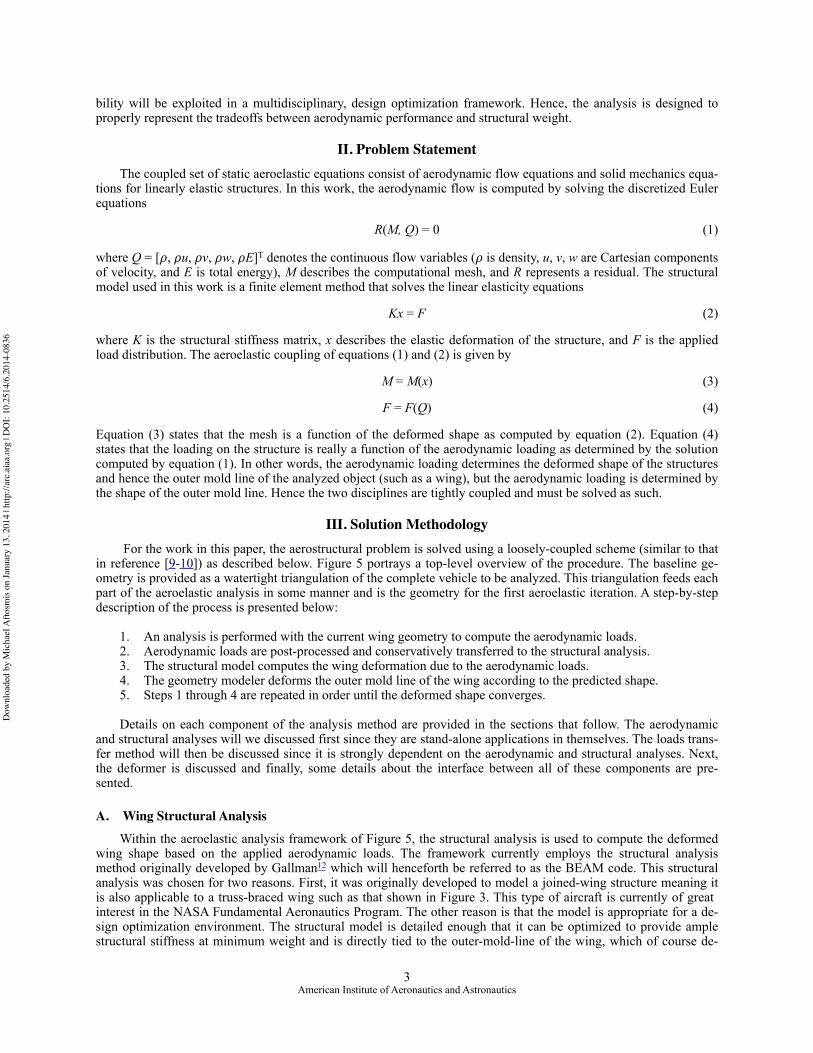
bending displacements, it is formally a three degree-of-freedom beam model. Like any finite-element model, accuracy is improved as the number of panels increases. Reference [12] suggests that 20 to 30 panels are enough resolution for a transport wing structure, and our experi-ence with the code concurs.

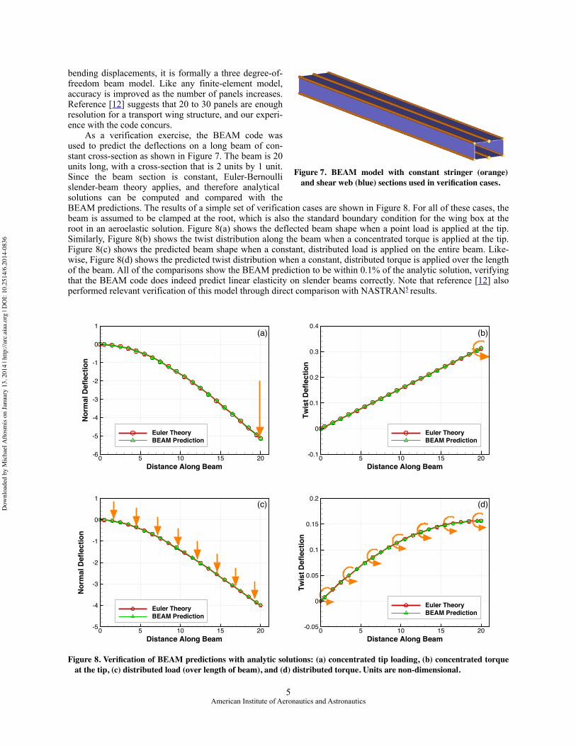
As a verification exercise, the BEAM code was used to predict the deflections on a long beam of con-stant cross-section as shown in Figure 7. The beam is 20 units long, with a cross-section that is 2 units by 1 unit. Since the beam section is constant, Euler-Bernoulli slender-beam theory applies, and therefore analytical solutions can be computed and compared with the BEAM predictions. The results of a simple set of verification cases are shown in Figure 8. For all of these cases, the beam is assumed to be clamped at the root, which is also the standard boundary condition for the wing box at the root in an aeroelastic solution. Figure 8(a) shows the deflected beam shape when a point load is applied at the tip. Similarly, Figure 8(b) shows the twist distribution along the beam when a concentrated torque is applied at the tip. Figure 8(c) shows the predicted beam shape when a constant, distributed load is applied on the entire beam. Like-wise, Figure 8(d) shows the predicted twist distribution when a constant, distributed torque is applied over the length of the beam. All of the comparisons show the BEAM prediction to be within 0.1% of the analytic solution, verifying that the BEAM code does indeed predict linear elasticity on slender beams correctly. Note that reference [12] also performed relevant verification of this model through direct comparison with NASTRAN5 results.


Distance Along Beam

Nor

mal

Def

lect

ion

0 5 10 15 20-6

-5

-4

-3

-2

-1

0

1

Euler TheoryBEAM Prediction

Distance Along Beam

Twis

t Def

lect

ion

0 5 10 15 20-0.1

0

0.1

0.2

0.3

0.4


Distance Along Beam

Nor

mal

Def

lect

ion

0 5 10 15 20-5

-4

-3

-2

-1

0

1


Distance Along Beam

Twis

t Def

lect

ion

0 5 10 15 20-0.05

0

0.05

0.1

0.15

0.2


Figure 8. Verification of BEAM predictions with analytic solutions: (a) concentrated tip loading, (b) concentrated torque at the tip, (c) distributed load (over length of beam), and (d) distributed torque. Units are non-dimensional.

(a) (b)

(c) (d)

Figure 7." BEAM model with constant stringer (orange) and shear web (blue) sections used in verification cases.

Dow

nloa

ded

by M

icha

el A

ftosm

is on

Janu

ary

13, 2

014

| http

://ar

c.ai

aa.o

rg |

DO

I: 10

.251

4/6.

2014

-083

6

B. Aerodynamic Analysis

Aerodynamic analysis for all results in this paper is performed using the Cart3D13 simulation package which includes an adjoint-driven mesh refinement capability. The package uses a Cartesian cut-cell approach14 in which the Euler equations (equation (1)) are discretized on a multilevel Cartesian mesh with embedded bounda-ries. The mesh consists of regular Cartesian hexahedra everywhere, except for a layer of body-intersecting boundary cells. The spatial discretization uses a second-order accurate finite volume method with a weak impo-sition of boundary conditions. The flux-vector splitting approach of van Leer15 is used. Steady-state flow solu-tions are obtained using a five-stage Runge–Kutta scheme with local time stepping and multigrid. Domain decomposition via space-filling curves permits parallel computation; for more details see Aftosmis et al. and Berger et al.16-18

Although it consists of nested Cartesian cells, the mesh is viewed as an unstructured collection of control volumes making the approach well-suited for solution-adaptive mesh refinement. Mesh refinement is based on a duality-preserving discrete adjoint solver developed by Nemec et al.19 While originally developed for gradient-based shape optimization,20 the method is also employed for error estimation and adaptive mesh refinement.21 The adjoint-based error-estimation tailors the mesh refinement to reduce discretization error in a user-selected output of interest such as lift or drag. Error in a functional can be either driven below some pre-specified value, or alternatively, reduced as much as possible using a “worst-errors-first strategy” until attaining a desired mesh size. Typical simulations cost 3-5 times that of a single flow solve on the final mesh. An example refined mesh and solution is depicted in Figure 9 for a case where mesh refinement was driven by both lift and drag. Another valuable Cart3D feature is the ability to specify a value of lift coefficient by iterating on the freestream angle of attack during the simulation.

Referring back to Figure 5, once a flow solution is computed, the surface pressure distribution is used to com-pute the distributed loads and moments on the wing surface. These loads and moments are then transferred to the structures model to compute deflections and therefore the deformed shape. More details on the transfer process are provided in the next section.

C. Loads Computation and Transfer

The structural model idealizes the wing structure as a tapered wing box, which in turn is modeled as a cantilever beam with a user-specified number of spanwise elements. This greatly simplifies the load-transfer process described in equation (4) as only the distribution of loads along the elastic axis is required. To obtain this distribution, the sur-face triangulation is partitioned into regions that correspond to the elements of the structural model. Once identified, the triangles in these partitions are then explicitly bound to the structural elements. This binding of the wing skin to the structural elements persists throughout the iterative process of the aeroelastic analysis portrayed in Figure 5. This is important since for cases with deflections greater than a few percent span, the same partitioning of the wing sur-face must be used throughout the iterative process for consistency.

The binding of the triangulation to the structural model is accomplished through the set of continuous strips whose boundaries are defined by the extended edges of the structural model elements. The strip boundaries are per-pendicular to the elastic axis of the wing with two exceptions. Near the wing root, everything inboard of the out-board edge of the root structural panel is included in that element’s binding. Similarly, at the wing tip, all of the sur-face outboard of the inboard edge of the tip panel is used to compute the load for that element. In other words, each triangle on the wing surface is bound to its nearest structural model panel. For a triangle whose area straddles more than one structural element, the centroid of that triangle is used to determine to which structural element it is bound. While this convention usually creates a “saw-tooth” edge between strips of triangles, any error introduced by this rougher boundary always vanishes as the surface triangulation is refined. Figure 10 gives an example where the dif-ferent colors indicate the partitioned bindings to a 10 element structural model.

The specific loads computed on each triangulation strip include the force component normal to and the moment about the elastic axis of the structural model. Referring back to Figure 5, these strip loads are applied to the corre-sponding beam element in the structural model. Recall that even as the wing deforms, the surface-triangle binding


Figure 9. Example of an adaptively-refined Cart3D mesh about a transport aircraft. The mesh refinement was driven by the accompanying adjoint solver. The surface coloring corresponds to local pressure.

Dow

nloa

ded

by M

icha

el A

ftosm

is on

Janu

ary

13, 2

014

| http

://ar

c.ai

aa.o

rg |

DO

I: 10

.251

4/6.

2014

-083

6

persists throughout the iterative computation. This means the binding only needs to be performed once as a pre-processing step.

Another feature of the load-transfer process is that the aerodynamic loads on the structural elements are always computed in the local axis system that is aligned with the current elastic axis shape. Figure 11 illustrates this notion. The force component computed and then applied to each structural element (based on the explic-itly bound region of the triangulation) is always taken normal to the current deformed shape of the wing. These are the loads that are applied to the undeformed struc-tural model to determine the latest shape of the de-formed wing. This is a first step to modeling nonlinear-ity in the aeroelastic solution of very flexible wings. If the structural model could directly compute additional, higher-order deformations due to forces on an already deformed wing, the method would be fully nonlinear (assuming linear elasticity, of course).

D. Deformation Scheme

The most important requirement of any deformer to be used in the aeroelastic analysis procedure is that it should mimic how a wing under load deforms in reality. This requirement is particularly necessary for cases with sizable deformations where the small angle approximations used in some traditional methods are no longer valid. The wing on the Boeing 787 (recall Figure 1) exhibits a sizable deformation of 10% semispan, for instance, and so a computational deformation scheme must properly capture the shape of this loaded wing. This section describes the deformer requirements in more detail and then discusses the choice and implementation of the deformation scheme used in the aeroelastic analysis procedure.

The ribs of a typical aircraft wing structure can be assumed to be mostly rigid since their sole purpose, after all, is to maintain the shape of the wing section. On a typical transport wing, these ribs are usually aligned to be perpen-dicular to the elastic axis of the entire structure. Hence, a deformer for the aeroelastic analysis should try to maintain the section shape normal to the elastic axis as it deflects the wing. There are several other geometric constraints nec-essary for a realistic deformation. Since spanwise extension or compression is assumed to be negligible, the de-former should maintain the wing span even as the spanwise shape is modified. This means that when the wing tip deflects normal to the spanwise direction, it also deflects inboard to keep the arc-length of the elastic axis constant. Analogous to maintaining the shape of the wing sections, the wing thickness normal to the elastic axis should also remain constant as the wing is deformed. Therefore, when the wing spanwise shape is modified, the wing sections normal to the elastic axis should roll and yaw appropriately.

The deformer used in this work is Blender,22 which is an open-source, discrete geometry engine that was origi-nally designed for computer graphics modeling and animation. Many of the deformation tools that are used in 3-D animation are also used in some form in modern shape optimization methods for aerospace designs. Blender also has an incredibly practical graphical-user-interface allowing the user to easily generate, modify, and deform discrete representations of nearly any geometric object. Since batch-mode manipulation and rendering is essential to 3-D


Figure 11. Force vectors computed along the span of a deformed wing (vectors shown on only a few panels for clarity). Note the vectors are normal to the local elastic axis of the wing structure.

Figure 10. Example binding of surface triangles to each structural element as indicated by different colors on the wing.

Dow

nloa

ded

by M

icha

el A

ftosm

is on

Janu

ary

13, 2

014

| http

://ar

c.ai

aa.o

rg |

DO

I: 10

.251

4/6.

2014

-083

6

animation, the package also provides a powerful Python-based23 application-programming-interface (API) allow-ing users to develop their own extensions and scripts. The surface deformer for the aeroelastic analysis proce-dure is built using Blender and this API.

Blender’s lattice modifier performs the actual de-formation of the triangulation. The lattice was chosen because it can satisfy all of the geometric constraints discussed above. Examples of lattice modifiers are shown in Figures 12 and 13. The lattice is initially a three-dimensional, strictly Cartesian mesh in space which is bound to a discrete geometry. As the vertices (or points) of the lattice are moved, the bound discrete geometry is morphed through 3-D spline functions de-fined between lattice points in the three Cartesian direc-tions aligned with the lattice. More details and examples of applying lattices to morph discrete geometry are pre-sented by Anderson.24

As shown in Figures 12 and 13, the lattices have only two vertices in dimensions that are not spanwise and hence are really a stack of simple rectangles. These lattices are also aligned so that the normals of the rec-tangles are parallel to the wing elastic axis. This means that displacements computed by the structural model are also the displacements of the lattice rectangles. To main-tain the wing section shape normal to the elastic axis, the lattice can be simply a spanwise array of rigid rec-tangles. Thus, the bound sectional shape parallel to the rectangles is always preserved even as the wing span-wise shape is modified. Conversely, in the direction along the elastic axis, a cubic Hermite spline function (more specifically a Catmull-Rom spline) is used to smoothly deform the wing surface between the many lattice sections. Note that this spline was not originally in the Blender distribution but has since been added to the application by the first author.*

The translational and rotational displacements that are computed by the structures code are also discrete in that values are predicted for the centroids of the beam elements and the very ends of the wing box. These locations are not always convenient since the Blender lattice consists of equally spaced points. Therefore, to generate a continu-ous function of the displacements, the discrete values are splined with a traditional cubic spline that enforces con-tinuous curvature. Figure 14 shows an example of computed discrete displacement values (the dots) along with their corresponding splines (red curves). The specific values that are splined are two components of beam deflection nor-mal to and the torque-driven rotation about the wing elastic axis. While these are the only displacements that are computed by the structural model, displacements and rotations in the other directions can also be computed to pre-serve geometric integrity. For instance, as the wing tip is deflected vertically, the wing tip moves inboard to preserve the actual wing span. Simply shearing the wing shape vertically would actually lengthen the wing span in terms of arc-length and unrealistically increase the wing area. Similarly, as the wing bends, the local section roll angle (or dihedral) must remain perpendicular to the deformed elastic axis or the effective wing thickness is altered due to unrealistic shearing of the geometry. This is demonstrated in the example in Figure 12; notice that the lattice sections remain perpendicular to the wing elastic axis even though it is bent. Likewise, as the wing is deflected in the streamwise direction, the lattice sections yaw to remain orthogonal to the elastic axis.

While Figures 12 and 13 show lattices with roughly 20 spanwise vertices, typically lattices are built with 64 spanwise rectangles which is the maximum lattice dimension allowed in Blender. This dimension is chosen to mini-mize interpolation error by the lattice splines. As discussed above, all six components of translation and rotation can be computed at any point along the span using the continuous displacement splines computed with the structural analysis results and geometric integrity constraints. Therefore, to apply the deformation with the lattice, the local


* Included in standard distribution since Blender 2.68.

Figure 13. Example deformation of a wing with a Blender lattice modifier. Note the lattice is aligned with the elastic axis of the wing consistent with the structural model.

Figure 12. Example deformation of a wing with a Blender lattice modifier. Note the spanwise sections of the lattice are rolled to preserve orthogonality to the deflected elastic axis and hence also preserve the local thickness.

Dow

nloa

ded

by M

icha

el A

ftosm

is on

Janu

ary

13, 2

014

| http

://ar

c.ai

aa.o

rg |

DO

I: 10

.251

4/6.

2014

-083

6

displacements are computed for each spanwise lattice section according to the displacement splines and constraints. From there, Blender produces a smoothly morphed surface triangulation that matches the deformed shape predicted by the structures model. This deformed geometry is used to build the computational mesh for the next aerodynamic analysis addressing equation (3), thereby completing the iterative cycle in the Figure 5 framework. The aeroelastic cycle converges when the difference between the de-formed geometries from consecutive iterations vanishes.

One other detail must be addressed for this defor-mation scheme. For a swept wing, the lattice often exists well into and even beyond the fuselage, as is the case in Figure 13. While only the wing part of the triangulation is bound to the lattice, an additional module was built for Blender that would smoothly fade the deflected wing geometry into the baseline geometry thereby preserving the intersection of the wing and fuselage. This is accom-plished by “blending” the baseline and deflected wings with the weighting functions shown in Figure 15. Note the functions are designed to always sum to unity. The spanwise extent over which this blending is applied was selected by aesthetics and the desire to minimize the influence of the blending. Blending that occurs too quickly can create very highly kinked geometry near the wing intersection, while blending too slowly reduces the actual influence of the structural model solution.

To apply the blending, each vertex on both the base-


DLR Dec 6, 2013

Wing-Fuselage Junction Preservation

• Lattice induced deflection extends into fuselage, corrupting wing junction

• Junction preserved by blending original into deflected wing with weighting functions

11

0

0.2

0.4

0.6

0.8

1.0

0 0.05 0.10 0.15 0.20

Wei

ghtin

g

Distance from Fuselage / Semispan

Undeflected WingDeflected Wing

Figure 15. Weighting function used for blending baseline and deflected wings to maintain valid geometry near the root. Note the abscissa is the fractional spanwise distance from the wing intersection with the fuselage.

Figure 14. Example of splined displacements computed by structures model. Note that for these plots, the Z-axis is aligned with the elastic axis of the wing, and the X-axis is chordwise. Note this image is an actual screen capture of optional output from the aeroelastic analysis interface, giving the user valuable feedback during the analysis. All plots are shown in the units of length consistent with the sample case.

discrete solutionsplined function

Dow

nloa

ded

by M

icha

el A

ftosm

is on

Janu

ary

13, 2

014

| http

://ar

c.ai

aa.o

rg |

DO

I: 10

.251

4/6.

2014

-083

6

line and deflected wings is weighted by these functions based on the baseline vertex location in the spanwise direction (normal to the freestream direction in this case) and then summed to create a new wing. This blended wing follows the predicted deflection for most of its span, but remains constrained near the root section. This process not only maintains valid geometry, but it also better represents reality where the wing is clamped at the root. While in actuality the fuselage also deforms a small amount, this effect is not currently modeled. Clamping the wing everywhere at the root provides a realistic model while preserving valid geometry at the wing-fuselage junction. The trailing edges of a baseline, de-flected, and blended wing near the root of an example wing-fuselage configuration are shown in Figure 16. The blended wing by itself is shown in Figure 17 for clarity.

E. Interface

All of the components shown in Figure 5 and dis-cussed in the sections above are modular, stand-alone applications. To control the transfer of data between components and the overall execution of the method, an interface consisting of Python modules and scripts was developed. The choice of scripting language was rational since the Blender API is also in Python. The interface provides the user with the ability to execute the entire scheme as shown in Figure 5 or just individual modules for unit testing. The modules that require the use of the Blender application can be executed in a manner where the results are presented within the Blender graphical-user-interface. All of these features enhance and acceler-ate a problem setup and debugging process. Other mod-ules that do not require Blender generate data files which can be viewed by many visualization packages. The interface also keeps track of convergence of the “aeroe-lastic iteration” (defined in Figure 5) by outputting the wing tip deflection computed during each cycle. Using Py-thon scripts and modules also allows the user to modify and therefore customize the process if necessary. This in-cludes the ability to substitute, enhance, and even include other modules or disciplines in the analysis.

IV. ApplicationsThe aeroelastic analysis tool was applied to two configurations as a demonstration and to provide preliminary

validation of the method. The first configuration is the HIgh REynolds Number AeroStructural Dynamics model (HIRENASD)25 which was tested in the European Transonic Wind Tunnel (ETW). This configuration was also adopted as a test case in the first Aeroelastic Prediction Workshop (AePW).26 It is one of the few available tests that provided static aeroelastic data, though the model was quite stiff. The second configuration analyzed was a Generic Transport Model (GTM)27 which was tested recently in the University of Washington Aeronautical Laboratory (UWAL) wind tunnel. This wind tunnel model was built to be twice as flexible as a Boeing 757 and is therefore an excellent validation case.

A. High Reynolds Number Aerostructural Dynamics Model (HIRENASD)

The first AePW was held in 2012 just before the AIAA 53rd Structures, Structural Dynamics and Materials Conference in Honolulu, HI. While most of the analysis tasks requested for the workshop involved forced, unsteady motion, one task also involved validation against static-aeroelastic experimental data. The HIRENASD wing, as shown in Figure 18, was tested in the ETW at transonic conditions and relatively high Reynolds numbers in 2006. Although the model was structurally quite stiff, the wing still exhibited notable wing-tip deflection at transonic con-ditions which induced noticeable changes in lift. The availability of validated simulation results from the workshop along with some published experimental data made this a good validation case for the aeroelastic analysis tool.


Figure 17. The blended wing from Figure 16.

Figure 16. Example of baseline (blue), deflected (gold), and blended (gray) wings portraying the effects of the weighting function in Figure 15. The view is upstream looking at the trailing edge with the fuselage on the left.

Dow

nloa

ded

by M

icha

el A

ftosm

is on

Janu

ary

13, 2

014

| http

://ar

c.ai

aa.o

rg |

DO

I: 10

.251

4/6.

2014

-083

6

For the AePW participants, a NASTRAN5 model of the wind tunnel test article was provided, which was used to create a BEAM model that exhibited the same flexibility in the flapping direction (normal to the wing chord). Because the wing tip deflection in the wind tun-nel is only about 1% semispan and the model was known to be very stiff in torsion, deflections due to tor-sional and streamwise loading are assumed to be negli-gible. Hence, the streamwise bending and torsional stiff-nesses are assumed to be very high and to not contribute to the aeroelastic solution.

To create the BEAM model, several loading condi-tions were applied to the NASTRAN model to measure deflections. Using this deflection data, a BEAM model was built so that when loaded, the predicted deflected shape matched that from the NASTRAN model. Several test cases were run to compare the predictions from the BEAM and NASTRAN models (see Figure 19). These plots compare predictions from the NASTRAN and BEAM models for various loading conditions. The agreement is quite good for all the test cases indicating that the BEAM model accurately captures the flapping stiffness distribution of the NASTRAN model.

Using this BEAM model, the Cart3D-based aeroe-lastic solver was used to analyze the HIRENASD ge-ometry at two conditions, namely those for ETW test runs 155 and 159 corresponding to freestream Mach numbers of 0.7 and 0.8. Both experiments report data for an angle of attack of 1.5°. Unfortunately, appropriately-vetted forces and deflection data were not made available for these tests and therefore direct comparisons with ex-perimental data were not possible. However, most participants of the AePW analyzed these conditions with Navier-Stokes-based aeroelastic analysis methods. NASA Langley provided deformed wing solutions (described in refer-ence [28]) that were generated using FUN3D.29 These high-fidelity solutions are thus used for code-to-code com-parisons of the Cart3D-based tool for these test cases.

Because viscous effects are significant for this wing at these conditions, the FUN3D-computed lift (and there-fore overall wing loading) was matched instead of angle of attack. This resulted in a slightly lower angle of attack in the Cart3D solutions. The angles of attack and computed lift of the Cart3D- and FUN3D-based aeroelastic analyses for the two cases are shown in Tables I and II. As expected, the Mach 0.7 solution required a smaller reduction in angle of attack to match lift than the Mach 0.8 case since the flow is nearly shock-free at Mach 0.7. The histories of the tip deflection as a function of aeroelastic iteration for both cases are shown in Figures 20-21. Both cases required only a few iterations to converge over two orders of magnitude. The computed deflected shapes for both test cases are shown in Figures 22-25 as compared to the rigid and FUN3D-computed geometries. What is shown are planar slices of the wing outer-mold-line near the elastic axis. The agreement between the Cart3D and FUN3D geometries is quite good. Moreover, though the experimental data is not officially available, reference [30] reports that the ex-perimentally measured tip deflection for the Mach 0.8 case is around 12 mm. This is also in good agreement with the Cart3D and Fun3D predicted deflection of 13mm (see Figure 25).

These results suggest that perhaps viscous effects may not need to be modeled in some cases to obtain the cor-rect wing deformation as long as the total load on the wing is correct. It may be possible to use an Euler-based ae-roelastic solver to compute the deformed shape of a loaded aircraft wing, and then use a viscous solver to compute


Figure 18. HIRENASD test article mounted in the ETW.

CFD Analysis Angle of Attack Lift Coefficient

FUN3D 1.5° 0.2951

Cart3D 1.44° 0.2952

Table I. Computed lift values on the HIRENASD wing at Mach 0.7, corresponding to ETW test run 155.

CFD Analysis Angle of Attack Lift Coefficient

FUN3D 1.5° 0.3038

Cart3D 1.31° 0.3043

Table II. Computed lift values on the HIRENASD wing at Mach 0.8, corresponding to ETW test run 159.

Dow

nloa

ded

by M

icha

el A

ftosm

is on

Janu

ary

13, 2

014

| http

://ar

c.ai

aa.o

rg |

DO

I: 10

.251

4/6.

2014

-083

6

the details of the flow more precisely. This process would obviously be much quicker than using the viscous solver repeatedly in a framework such as the one shown in Figure 5 since an Euler solver is nominally 1-2 orders of magni-tude cheaper in terms of computation costs. Employing a Cartesian-mesh solver is even more attractive since mesh-ing is automatic whereas most viscous solvers would require some sort of volume mesh deformation scheme.


Aeroelastic Iteration

Tip

Def

lect

ion

/ Sem

ispa

n

0 1 2 3 4 5 6 7 80.000

0.002

0.004

0.006

0.008

0.010

0.012

0.014

0.016


|6 T

ip D

efle

ctio

n| /

Sem

ispa

n

0 1 2 3 4 5 6 7 810-6

10-5

10-4

10-3

10-2

10-1

Figure 20. Convergence of the aeroelastic analysis for the HIRENASD test article at Mach 0.7.

Distance Along Elastic Axis (m)

Nor

mal

Def

lect

ion

(m)

0.2 0.4 0.6 0.8 1.0 1.2 1.4 1.60.00

0.01

0.02

0.03

0.04

0.05

BEAMNASTRAN

1500 N


Nor

mal

Def

lect

ion

(m)

0.2 0.4 0.6 0.8 1.0 1.2 1.4 1.60.00

0.01

0.02

0.03

0.04

0.05

BEAMNASTRAN

2000 N


Nor

mal

Def

lect

ion

(m)

0.2 0.4 0.6 0.8 1.0 1.2 1.4 1.60.00

0.01

0.02

0.03

0.04

0.05

BEAMNASTRAN 2000 N

2000 N


Nor

mal

Def

lect

ion

(m)

0.2 0.4 0.6 0.8 1.0 1.2 1.4 1.60.00

0.01

0.02

0.03

0.04

0.05

BEAMNASTRAN

1500 N

2000 N

1000 N

Figure 19. Comparison of normal displacement as predicted by BEAM and NASTRAN models when the HIRENASD test article is loaded (a) at three-quarters span, (b) at the tip, (c) midspan and at the tip, and (d) at 3 locations.

(a) (b)

(c) (d)

Dow

nloa

ded

by M

icha

el A

ftosm

is on

Janu

ary

13, 2

014

| http

://ar

c.ai

aa.o

rg |

DO

I: 10

.251

4/6.

2014

-083

6


Figure 25. Rigid and deformed wing tip geometries as computed by Cart3D and FUN3D aeroelastic analyses at Mach 0.8.

Figure 24. Rigid and deformed wing tip geometries as computed by Cart3D and FUN3D aeroelastic analyses at Mach 0.7.

Figure 23. Rigid and deformed geometries as computed by Cart3D and FUN3D aeroelastic analyses at Mach 0.8.

Figure 22. Rigid and deformed geometries as computed by Cart3D and FUN3D aeroelastic analyses at Mach 0.7.


Tip

Def

lect

ion

/ Sem

ispa

n

0 1 2 3 4 5 6 7 80.000

0.002

0.004

0.006

0.008

0.010

0.012

0.014

0.016


|6 T

ip D

efle

ctio

n| /

Sem

ispa

n

0 1 2 3 4 5 6 7 810-6

10-5

10-4

10-3

10-2

10-1

Figure 21. Convergence of the aeroelastic analysis for the HIRENASD test article at Mach 0.8.

Dow

nloa

ded

by M

icha

el A

ftosm

is on

Janu

ary

13, 2

014

| http

://ar

c.ai

aa.o

rg |

DO

I: 10

.251

4/6.

2014

-083

6

B. Generic Transport Model (GTM)

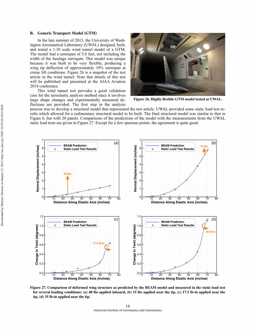
In the late summer of 2013, the University of Wash-ington Aeronautical Laboratory (UWAL) designed, built, and tested a 1:10 scale wind tunnel model of a GTM. The model had a semispan of 5.6 feet, not including the width of the fuselage surrogate. This model was unique because it was built to be very flexible, producing a wing tip deflection of approximately 10% semispan at cruise lift conditions. Figure 26 is a snapshot of the test article in the wind tunnel. Note that details of this test will be published and presented at the AIAA Aviation 2014 conference.

This wind tunnel test provides a good validation case for the aeroelastic analysis method since it involves large shape changes and experimentally measured de-flections are provided. The first step in the analysis process was to develop a structural model that represented the test article. UWAL provided some static load test re-sults which allowed for a rudimentary structural model to be built. The final structural model was similar to that in Figure 6, but with 20 panels. Comparisons of the predictions of the model with the measurements from the UWAL static load tests are given in Figure 27. Except for a few spurious points, the agreement is quite good.


Distance Along Elastic Axis (inches)

Nom

ral D

ispl

acem

ent (

inch

es)

0 10 20 30 40 50 60 70 800

1

2

3

4

5

6

7

BEAM PredictionStatic Load Test Results

40 lbs


Nor

mal

Dis

plac

emen

t (in

ches

)

0 10 20 30 40 50 60 70 800

1

2

3

4

5

6

7


15 lbs


Cha

nge

in T

wis

t (de

gree

s)

0 10 20 30 40 50 60 70 800.0

0.2

0.4

0.6

0.8

1.0

1.2


17.5 lb-in


Cha

nge

in T

wis

t (de

gree

s)

0 10 20 30 40 50 60 70 800.0

0.2

0.4

0.6

0.8

1.0

1.2


35 lb-in

Figure 27. Comparison of deformed wing structure as predicted by the BEAM model and measured in the static load test for several loading conditions: (a) 40 lbs applied inboard, (b) 15 lbs applied near the tip, (c) 17.5 lb-in applied near the tip, (d) 35 lb-in applied near the tip.

(a) (b)

(c) (d)

Figure 26. Highly flexible GTM model tested at UWAL.

Dow

nloa

ded

by M

icha

el A

ftosm

is on

Janu

ary

13, 2

014

| http

://ar

c.ai

aa.o

rg |

DO

I: 10

.251

4/6.

2014

-083

6

The GTM wind tunnel model was analyzed at the same conditions as one of the test runs. The tunnel dy-namic pressure for this case was 20 lbs/ft2 at sea level conditions, which resulted in a freestream Mach num-ber of 0.12. A full sweep of incidence angles was ana-lyzed using the coupled aeroelastic analysis. To high-light the effects of the wing deformation, the rigid (un-deformed) wing was also analyzed. The results of these analyses along with the wind tunnel measurements are shown in Figure 28. Note the tremendous over-prediction (roughly 25%) of lift by the rigid wing at high angles of attack, while the aeroelastic solution matches the measured lift almost exactly.

The wind tunnel data also provides wing deflec-tions at certain points along the span of the wing. For a more detailed validation, one of these test runs was selected as an additional test case for the aeroelastic analysis tool. The condition selected had a measured, corrected angle of attack of 5.38° that corresponds closely to the design cruise lift coefficient of 0.51. Once converged, the deflected shape of the wing elastic axis (based on the structural model) was extracted and com-pared to the wind tunnel data as shown in Figure 29. The agreement is good, which obviously helps explain the good agreement in Figure 28. Note that the elastic axis of the structural model is not exactly in the same chordwise location as that of the measured deflections in the wind tunnel test though it is very close (within 5-10% chord). Also, based on the data shown in Fig-ure 27, the model is rather stiff torsionally. This means very little twist is induced by the aerodynamic loads and therefore the difference in chordwise location of the measured deflection and the structural model elastic axis is less significant.

As was the case for the HIRENASD configuration, the convergence of GTM test case was very rapid. The history of the tip deflection with respect to the number of aeroelastic iterations is shown in Figure 30. Here the tip deflection converges over 4 orders of magnitude in a handful of aeroelastic iterations.



Tip

Def

lect

ion

/ Sem

ispa

n

0 1 2 3 4 5 6 7 80.00

0.02

0.04

0.06

0.08

0.10

0.12

0.14

0.16


|6 T

ip D

efle

ctio

n| /

Sem

ispa

n

0 1 2 3 4 5 6 7 810-7

10-6

10-5

10-4

10-3

10-2

10-1

100

Figure 30. Convergence of the aeroelastic analysis for the GTM test article at 5.38° angle of attack.

angle of attack (degrees)

Lift

Coe

ffici

ent

-4 -2 0 2 4 6 8-0.1

0

0.1

0.2

0.3

0.4

0.5

0.6

0.7

0.8

Cart3D - rigid wingCart3D - aeroelastic wingUWAL Test - Run 104

Figure 28. Comparison of lift coefficients on the GTM as measured in the UWAL test and as computed by Cart3D, both on the rigid wing and the aeroelastic wing.

Spanwise Location (inches)

Nor

mal

Def

lect

ion

(inch

es)

0 10 20 30 40 50 60 700

1

2

3

4

5

6

7

Cart3D Aeroelastic PredictionUWAL Test - Run 23

Figure 29. Comparison of measured (UWAL wind tunnel test) and predicted (Cart3D-based aeroelastic analysis) wing deflections at 5.38° angle of attack.

Dow

nloa

ded

by M

icha

el A

ftosm

is on

Janu

ary

13, 2

014

| http

://ar

c.ai

aa.o

rg |

DO

I: 10

.251

4/6.

2014

-083

6

Unlike the HIRENASD case discussed in the previous subsection, the GTM solutions did not show significant viscous effects as indicated by the fact that lift was computed so accurately as a function of angle of attack (see Fig-ure 28). For this case, it is quite probable that a viscous-solver-based aeroelastic solution would compute very nearly the same deformed shape as what was computed with the Euler solver. This is further evidence that perhaps viscous effects need not be addressed to get a deformed wing geometry that is very close to reality. Naturally, a great deal more research is necessary to verify this hypothesis, but these initial results are encouraging nonetheless.

V. ConclusionsA simple structural model, a Cartesian-mesh Euler solver, and a discrete geometry engine have been loosely

coupled to spawn an application capable of performing static, aeroelastic analysis on highly flexible aircraft wings. The application was designed to be modular to allow for analysis swapping, module testing, and easy problem setup. The structural model was verified with Euler beam theory for several loading conditions in both bending and twist. The Euler solver with its adjoint-based mesh adaptation capability allowed for good convergence of aeroelastic simulations. The procedure has been observed to converge quickly despite its loose coupling, requiring only a few iterations to converge the predicted change in the wing shape 2-3 orders of magnitude. The application has also been demonstrated to be accurate for the two test cases presented. The first case involved a structurally stiff wind tunnel model of a transport wing in transonic flow. By matching lift, viscous effects were lessened and the small deflections in this case were accurately predicted as compared to both published RANS-based aeroelastic solutions and experi-mental data. This result suggests that perhaps a viscous solver may not be necessary to obtain a very close approxi-mation to a wing’s aeroelastic shape, even in transonic flow. The second case involved a very flexible wing in nearly incompressible flow. For this case, lift did not need to be matched as Reynolds number effects were not found to be significant. The simulated results matched the wind tunnel data very well. Accurately predicting the large deflections on a highly flexible wing instills significant confidence in the Cart3D-based aeroelastic analysis tool. Overall, these initial results suggest the method is accurate, converges quickly, and is applicable in several flight regimes.

In terms of the computational cost of the analysis method, the aerodynamic analysis component by far requires the most computer resources. The tapered-beam solver requires a minuscule amount of computer time as compared to the CFD simulation. On the other hand, because a BEAM model is built from the outer mold line of a triangula-tion by using the Blender API, this step often requires much more time than the actual structural analysis. Fortu-nately, this preprocessing step is only performed once per wing geometry and requires a only a small fraction of the resources needed by the flow solver in an aeroelastic analysis.

VI. Future WorkMore work is planned for the Cart3D-based aeroelastic analysis tool presented above to enhance its accuracy

and applicability. Though unnecessary for the two test cases presented above, the effects of gravity (wing structural weight) will be addressed in future versions of the tool. The effects of fuel and engine weights will also be ad-dressed. Also, the BEAM model can handle moments that are about axes not aligned with the elastic axis. These moments can be computed and added to the loads on the wing structure which may be important for some complex geometries. Of course, the aeroelastic analysis tool should not be limited to the BEAM structural model. Other struc-tural analyses should be available such as the simple finite element method used by Nguyen31 or even NASTRAN itself. Finally, in the more distant future, a dynamic aeroelastic analysis capability would be desirable for flutter and buffet-onset prediction. Such a tool would likely implement the time-tested techniques used by Guruswamy32 and Farhat.33

As these features are added to the solver, additional validation exercises will be performed to confirm the accu-racy of the method. Unfortunately, aeroelastic validation test cases are quite rare, especially those that are accompa-nied by experimental data. Of course, validating the method using solutions from other already-validated aeroelastic solvers would augment confidence in the methodology. Another interesting exercise would be to analyze the final geometry from a converged Cart3D-based aeroelastic solution with a viscous code such as FUN3D. Loads could then be extracted from the viscous solution and applied to the structural model to estimate how different a viscous aeroelastic solution would be from the inviscid one. Should the results of this exercise indicate that the inviscid solu-tion is sufficient to obtain the shape, then the process of obtaining a viscous solution on a loaded flexible wing could be made much more efficient by first using the faster Cart3D-based tool first.

Looking at the bigger picture, the aeroelastic analysis procedure provides the opportunity for aeroelastic design optimization of typical transport and even truss-braced wings. The adjoint-driven, design capability of Cart3D pro-vides a scheme for quickly computing aerodynamic performance sensitivities to geometric shape changes. The BEAM model was also selected to provide the capability to optimize the structural design itself. Working in tandem, the two analyses should properly represent the tradeoffs that exist in the design space of an aircraft wing, particu-larly for the very flexible designs of the future. Ultimately this method was created not just as a stand-alone analysis


Dow

nloa

ded

by M

icha

el A

ftosm

is on

Janu

ary

13, 2

014

| http

://ar

c.ai

aa.o

rg |

DO

I: 10

.251

4/6.

2014

-083

6

but more so to be exploited within a design optimization framework. While the exact architecture of such a frame-work has not been established, the development of the framework is currently planned for the near future.

VII. AcknowledgmentsThis work was supported by the NASA Ames Research Center contract NNA10DF26C and the Fixed Wing

project of NASA’s Fundamental Aeronautics Program. The authors would also like to acknowledge those who were instrumental in completing the work in this paper. George Anderson, a Ph.D. candidate at Stanford University, was extremely helpful by providing guidance in developing the Python-based interface which tapped the Blender API. Eric Ting and Nhan Nguyen of the Intelligent Systems Division at NASA Ames provided NASTRAN support and many helpful discussions. Pawel Chwalowski of the Aeroelasticity Branch at NASA Langley provided the FUN3D solutions used for validation.

References1Drela, M., “Development of the D8 Transport Configuration,” AIAA 2011–3970, June 2011. 2Bradley, M. K. and Droney, C. K., “Subsonic Ultra Green Aircraft Research Phase II: N+4 Advanced Concept Develop-

ment,” NASA CR-2012-217556, May 2012.3Urnes, J., Nguyen, N., Ippolito, C., Totah, J., Trihn, K., and Ting, E., “A Mission-Adaptive Variable Camber Flap Control

System to Optimize High Lift and Cruise Lift-to-Drag Ratios of Future N+3 Transport Aircraft,” AIAA 2013-0214, January 2013.4Albano, E. and Rodden, W. P., “A Doublet-Lattice Method for Calculating Lift Distributions on Oscillating Surfaces in

Subsonic Flows,” AIAA Journal, Vol. 7, No. 2, February 1969, pp. 279-285.5Rodden, W. P. and Johnson, E. H., MSC/NASTRAN Aeroelastic Analysis: User's guide, version 68, MacNeal-Schwendler

Corp., 1994.6Drela, M., “Method for Simultaneous Wing Aerodynamic and Structural Load Predictions,” AIAA 89-2200, June 1989.7Guruswamy, G. P., "Coupled Finite-Difference/Finite-Element Approach for Wing-Body Aeroelasticity," AIAA 92-4680-

CP, September 1992.8Chipman, R., Waters, C., and MacKenzie, D., “Numerical Computation of Aeroelastically Corrected Transonic Loads,”

AIAA 79-0766, January 1979.9Whitlow Jr., W. and Bennett, R. M., “Application of a Transonic Potential Flow Code to the Static Aeroelastic Analysis of

Three-Dimensional Wings," AIAA 82-0689, January 1982.10Tatum, K. E. and Giles, G., “Integrating Nonlinear Aerodynamic and Structural Analysis for a Complete Fighter Configu-

ration,” Journal of Aircraft, Vol. 25, No. 12, December 1988, pp. 1150-1156.11Martins, J. R. R. A., A Coupled-Adjoint Method for High-Fidelity Aero-Structural Optimization, PhD thesis, Stanford Uni-

versity, Stanford, CA, 2002.12Gallman, J. W. and Kroo, I. M., “Structural Optimization for Joined-Wing Synthesis,” Journal of Aircraft, Vol. 33, No. 1,

January-February 1996, pp. 214-223.13Aftosmis, M. J., Berger, M. J., and Adomavicius, G., “A Parallel Multilevel Method for Adaptively Refined Cartesian

Grids with Embedded Boundaries,” AIAA 2000-0808, January 2000.14Aftosmis, M. J., Berger, M. J., and Melton, J. E., “Robust and Efficient Cartesian Mesh Generation on Component Based

Geometry,” AIAA Journal, Vol. 36, No. 6, June 1998, pp. 952–960.15van Leer, B., “Flux-Vector Splitting for the Euler Equations,” ICASE Report 82-30, September 1982.16Aftosmis, M. J., Berger, M. J., and Adomavicius, G. D., “A Parallel Multilevel Method for Adaptively Refined Cartesian

Grids with Embedded Boundaries,” AIAA 2000-0808, January 2000.17Aftosmis, M. J., Berger, M. J., and Murman, S. M., “Applications of Space-Filling-Curves to Cartesian methods in CFD,”

AIAA 2004-1232, January 2004.18Berger, M. J., Aftosmis, M. J., and Murman, S. M., “Analysis of Slope Limiters on Irregular Grids,” AIAA 2005-0490,

January 2005.19Nemec, M., Aftosmis, M. J., Murman, S. M., and Pulliam, T. H., “Adjoint Formulation for an Embedded-Boundary Carte-

sian Method,” AIAA 2005-0877, January 2005.20Nemec, M. and Aftosmis, M. J., “Adjoint Sensitivity Computations for an Embedded-Boundary Cartesian Mesh Method,”

Journal of Computational Physics, Vol. 227, 2008, pp. 2724-2742.


Dow

nloa

ded

by M

icha

el A

ftosm

is on

Janu

ary

13, 2

014

| http

://ar

c.ai

aa.o

rg |

DO

I: 10

.251

4/6.

2014

-083

6

21Nemec, M. and Aftosmis, M. J., “Adjoint Error-Estimation and Adaptive Refinement for Embedded-Boundary Cartesian Meshes,” AIAA 2007–4187, June 2007.

22http://www.blender.org23http://python.org24Anderson, G. R., Aftosmis, M. J., and Nemec, M., “Constraint-based Shape Parameterization for Aerodynamic Design,”

ICCFD7-2001, July 2012.25Ballmann, J., Dafnis, A., Korsch, H., Buxel, C., Reimerdes, H. G., Brakhage, K. H., Olivier, H., Braun, C., Baars, A., and

Boucke, A., “Experimental Analysis of High Reynolds Number Aero-Structural Dynamics in ETW,” AIAA 2008-0841, January 2008.

26Heeg, J., Chwalowski, P., Florance, J. P., Wieseman, C. D., Schuster, D. M., and Perry, B., “Overview of the Aeroelastic Prediction Workshop,” AIAA 2013-0783, January 2013.

27Precup, N., “VCCTEF Wing Configuration Aeroelastic Wind Tunnel Model Construction, Geometry, and Test Procedures Information (Draft),” University of Washington Aeronautical Laboratory, September 2013.

28Chwalowski, P., Heeg, J., Wieseman, C. D., and Florance, J. P., “FUN3D Analyses in Support of the First Aeroelastic Pre-diction Workshop,” AIAA 2103-0785, January 2013.

29http://fun3d.larc.nasa.gov30Reimer, L., Boucke, A., Ballmann, J., and Behr, M., “Computational Analysis of High Reynolds Number Aero-Structural

Dynamics (HIRENASD) Experiment,” Int. Forum Aeroelastic Structural Dynamics (IFASD), 2009.31Nguyen, N. and Urnes, J., “Aeroelastic Modeling of Elastically Shaped Aircraft Concept via Wing Shaping Control for

Drag Reduction,” AIAA 2012-4642, August 2012.32Guruswamy, G. P., “Unsteady Aerodynamic and Aeroelastic Calculations for Wings Using Euler Equations,” AIAA Jour-

nal, Vol. 28, No. 3, 1990, pp. 461-469.33Farhat, C. and Lesoinne, M., “Enhanced Partitioned Procedures for Solving Nonlinear Transient Aeroelastic Problems,”

AIAA 98-1806, April 1998.


Dow

nloa

ded

by M

icha

el A

ftosm

is on

Janu

ary

13, 2

014

| http

://ar

c.ai

aa.o

rg |

DO

I: 10

.251

4/6.

2014

-083

6

http://www.blender.org

http://www.blender.org

http://python.org

http://python.org

http://fun3d.larc.nasa.gov

http://fun3d.larc.nasa.gov

Documents

Static Aeroelastic Analysis with an Inviscid Cartesian … · Static Aeroelastic Analysis with an Inviscid Cartesian Method David L. Rodriguez* Science & Technology Corp., Moffett