Embed Size (px)
Citation preview

STATE ESTIMATION FOR AUTONOMOUS FLIGHT
IN CLUTTERED ENVIRONMENTS
A DISSERTATION
SUBMITTED TO THE DEPARTMENT OF AERONAUTICS AND ASTRONAUTICS
AND THE COMMITTEE ON GRADUATE STUDIES
OF STANFORD UNIVERSITY
IN PARTIAL FULFILLMENT OF THE REQUIREMENTS
FOR THE DEGREE OF
DOCTOR OF PHILOSOPHY
Jacob Willem Langelaan
March 2006

c© Copyright by Jacob Willem Langelaan 2006
All Rights Reserved
ii

I certify that I have read this dissertation and that, in my opinion,
it is fully adequate in scope and quality as a dissertation for the
degree of Doctor of Philosophy.
Stephen M. Rock(Principal Adviser)
I certify that I have read this dissertation and that, in my opinion,
it is fully adequate in scope and quality as a dissertation for the
degree of Doctor of Philosophy.
Sanjay Lall
I certify that I have read this dissertation and that, in my opinion,
it is fully adequate in scope and quality as a dissertation for the
degree of Doctor of Philosophy.
Claire Tomlin
Approved for the University Committee on Graduate Studies.
iii

Abstract
SAFE, AUTONOMOUS OPERATIONin complex, cluttered environments is a critical challenge fac-
ing autonomous mobile systems. The research described in this dissertation was motivated by
a particularly difficult example of autonomous mobility: flight of a small Unmanned Aerial Vehicle
(UAV ) through a forest. The focus was on enabling the three critical tasks that comprise flight: (1)
maintaining controlled flight while avoiding collisions (aviate); (2) flying from a known start loca-
tion to a known goal location (navigate); and (3) providing information about the environment– a
map– to a human operator or other robots in the team (communicate).
In cluttered environments (such as forests or natural and urban canyons) signals from navigation
beacons such asGPS may be frequently occluded. Direct measurements of vehicle position are
therefore unavailable. Additionally, payload limitations of smallUAVs restrict both the mass and
physical dimensions of sensors that can be carried on board.
This dissertation describes the development and proof-of-concept demonstration of a naviga-
tion system that uses only a low-cost inertial measurement unit and a monocular camera. Micro
electromechanical inertial measurements units (IMUs) are well suited to smallUAV applications and
provide measurements of acceleration and angular rate. However, they do not provide information
about nearby obstacles (needed for collision avoidance) and their noise and bias characteristics lead
to unbounded growth in computed position. A monocular camera can provide bearings to nearby
obstacles and landmarks. These bearings can be used both to enable obstacle avoidance and to aid
navigation.
Presented here is a solution to the problem of estimating vehicle state (its position, orientation
and velocity) as well as the positions of obstacles or landmarks in the environment using only in-
ertial measurements and bearings to landmarks. This is a highly nonlinear estimation problem, and
standard estimation techniques such as the Extended Kalman Filter (EKF) are prone to divergence
in this application. In this dissertation a Sigma Point Kalman Filter (SP-KF) is implemented, result-
ing in an estimator which is able to cope with the significant nonlinearities in the system equations
and uncertainty in state estimates while remaining tractable for real-time operation. In addition,
the issues of data association and landmark initialization are addressed. Estimator performance is
iv

examined through Monte Carlo simulations in both two and three dimensions for scenarios involv-
ing UAV flight in cluttered environments. Hardware tests and simulations demonstrate navigation
through an obstacle-strewn environment by a small Unmanned Ground Vehicle.
v

To Maggie.
vi

Acknowledgments
No man is an island, entire of itself; every
man is a piece of the continent, a part of the
main.John Donne, Meditation XVII
Very few people perform their work in isolation. Over the five and a half years I spent at Stanford
I have relied on the help of many people, without whom this project would never have been finished.
First I thank my advisor, Professor Stephen Rock. By allowing us to find our own research
projects he sends us off on a long, tangled journey. At first glance it seems we wander randomly, but
in reality he guides us with careful hints and suggestions. This Socratic approach is both frustrating
and incredibly rewarding, and in the end it makes better researchers of all of us. Most importantly
I am grateful for the family-friendly environment he fosters, encouraging all of us with children to
take the time to watch them grow.
I am very grateful to my reading committee, Professor Claire Tomlin and Professor Sanjay
Lall. Thanks also to Professor Gunter Niemeyer for acting as defense committee chair. I greatly
appreciate all of their comments and suggestions.
The final member of my defense committee was Professor Robert Cannon, who founded the
ARL in 1984 with the idea of “putting smart people in a room, then standing back to watch what
happens”. It is an extraordinary place and I am grateful to have been a part of it.
Without the help of theARL ’s staff I would never have finished. Godwin Zhang’s expertise with
all things electronic is truly amazing. Sherann Ellsworth and Dana Parga made sure the lab was
running smoothly: without them all research in the Guidance and Controls groups would grind to a
halt. I also thank the Department’s graduate student services staff, Lynn Kaiser and Robin Murphy,
for making sure all my paperwork was completed on time.
One of the greatest aspects of theARL is the spirit of cooperation that exists among its students.
It was obvious as soon as I began the process of joining the lab. The senior grad students were
always available to talk about their research: the problems they were having, what they saw as good
next steps and how it complemented the work of other students in the lab. I am especially grateful
to Eric Frew, Andreas Huster, Hank Jones, and Jason Rife, four of the previous generation, for
helping me get started in the lab. Later, when I was in the midst of my research, Chris Clark and
vii

Tim Bretl could always ask the question that made me examine my work more carefully. Of my
generation, Aaron Plotnik and Kristof Richmond have helped enormously both with practical items
(without their image processing code I would have been here for months longer) and with many
many discussions of research direction.
While the working environment in the lab was wonderful, the best part of my day was coming
home to my family. My two daughters Hannah (now aged 3 3/4) and Ava (age 1) made the worst
days into good days. I once asked Hannah, “Where would I be without you?” She thought about it
for a second or two and then answered, “Lost.” I laughed and I cried– she spoke the truth.
Finally the greatest thanks go to my wife Maggie. She left her family and friends to drive 2600
miles with me as we started our adventure in far-off California. She will soon leave her friends in
California as we travel to a new adventure in Pennsylvania. She is my wife, my partner, my best
friend. I am ever-blessed with her and with the family that we have together.
viii

Contents
Abstract iv
Acknowledgments vii
1 Introduction 1
1.1 Motivation . . . . . . . . . . . . . . . . . . . . . . . . . . . . . . . . . . . . . . . 2
1.2 A Framework for Integrated Control and Navigation . . . . . . . . . . . . . . . . .4
1.3 The Estimation Problem . . . . . . . . . . . . . . . . . . . . . . . . . . . . . . .6
1.3.1 Preventing Estimator Divergence . . . . . . . . . . . . . . . . . . . . . . .7
1.3.2 Data Association . . . . . . . . . . . . . . . . . . . . . . . . . . . . . . . 8
1.3.3 Landmark Initialization . . . . . . . . . . . . . . . . . . . . . . . . . . . . 8
1.3.4 Additional Issues . . . . . . . . . . . . . . . . . . . . . . . . . . . . . . . 9
1.4 Related Work . . . . . . . . . . . . . . . . . . . . . . . . . . . . . . . . . . . . .10
1.4.1 Vision Based Navigation and Structure from Motion . . . . . . . . . . . .10
1.4.2 Simultaneous Localization and Mapping . . . . . . . . . . . . . . . . . . .12
1.4.3 Data Association . . . . . . . . . . . . . . . . . . . . . . . . . . . . . . .12
1.4.4 Landmark Initialization . . . . . . . . . . . . . . . . . . . . . . . . . . . .13
1.4.5 Sigma Point Kalman Filters . . . . . . . . . . . . . . . . . . . . . . . . .13
1.5 Summary of Contributions . . . . . . . . . . . . . . . . . . . . . . . . . . . . . .14
1.6 Reader’s Guide . . . . . . . . . . . . . . . . . . . . . . . . . . . . . . . . . . . .15
2 The State Estimation Problem 16
2.1 Problem Statement . . . . . . . . . . . . . . . . . . . . . . . . . . . . . . . . . .17
2.2 Sensor and System Models . . . . . . . . . . . . . . . . . . . . . . . . . . . . . .19
2.2.1 Coordinate Frames . . . . . . . . . . . . . . . . . . . . . . . . . . . . . .19
2.2.2 Vehicle Kinematic Model . . . . . . . . . . . . . . . . . . . . . . . . . .19
2.2.3 Inertial Measurement Model . . . . . . . . . . . . . . . . . . . . . . . . .21
2.2.4 Vision Model . . . . . . . . . . . . . . . . . . . . . . . . . . . . . . . . .22
2.3 Nonlinear Estimation . . . . . . . . . . . . . . . . . . . . . . . . . . . . . . . . .23
ix

2.3.1 Particle Filters . . . . . . . . . . . . . . . . . . . . . . . . . . . . . . . .24
2.3.2 Extended Kalman Filter . . . . . . . . . . . . . . . . . . . . . . . . . . .25
2.3.3 Sigma Point Filters . . . . . . . . . . . . . . . . . . . . . . . . . . . . . .26
2.3.4 Comparison of Techniques . . . . . . . . . . . . . . . . . . . . . . . . . .27
2.4 Summary: The Estimation Problem . . . . . . . . . . . . . . . . . . . . . . . . .30
3 Estimator Design 32
3.1 Inertial/Vision Navigation Filter . . . . . . . . . . . . . . . . . . . . . . . . . . .33
3.1.1 Prediction Step . . . . . . . . . . . . . . . . . . . . . . . . . . . . . . . .33
3.1.2 Vision Update . . . . . . . . . . . . . . . . . . . . . . . . . . . . . . . . .35
3.1.3 Choice of States . . . . . . . . . . . . . . . . . . . . . . . . . . . . . . .35
3.2 Data Association . . . . . . . . . . . . . . . . . . . . . . . . . . . . . . . . . . .36
3.3 Landmark Initialization . . . . . . . . . . . . . . . . . . . . . . . . . . . . . . . .38
3.4 Estimate Smoothing . . . . . . . . . . . . . . . . . . . . . . . . . . . . . . . . . .40
3.5 Data Flow . . . . . . . . . . . . . . . . . . . . . . . . . . . . . . . . . . . . . . .41
4 UAV Simulation Results 44
4.1 Navigation in a Plane . . . . . . . . . . . . . . . . . . . . . . . . . . . . . . . . .45
4.1.1 Estimate Consistency . . . . . . . . . . . . . . . . . . . . . . . . . . . . .46
4.1.2 System Equations for the Planar Case . . . . . . . . . . . . . . . . . . . .46
4.1.3 Monte Carlo Simulation Results . . . . . . . . . . . . . . . . . . . . . . .47
4.1.4 Navigation and Obstacle Avoidance . . . . . . . . . . . . . . . . . . . . .51
4.2 3D Simulations . . . . . . . . . . . . . . . . . . . . . . . . . . . . . . . . . . . .51
4.2.1 Estimator Performance . . . . . . . . . . . . . . . . . . . . . . . . . . . .54
4.2.2 Effect of Explicit Data Association and Landmark Initialization . . . . . .56
4.2.3 Discussion of 3D Simulation Results . . . . . . . . . . . . . . . . . . . . .59
4.3 Summary . . . . . . . . . . . . . . . . . . . . . . . . . . . . . . . . . . . . . . .62
5 Ground Vehicle Results 64
5.1 Hardware Implementation . . . . . . . . . . . . . . . . . . . . . . . . . . . . . .65
5.1.1 Vision Subsystem . . . . . . . . . . . . . . . . . . . . . . . . . . . . . . .65
5.1.2 Inertial Subsystem . . . . . . . . . . . . . . . . . . . . . . . . . . . . . .67
5.1.3 Path Planning and Control . . . . . . . . . . . . . . . . . . . . . . . . . .67
5.2 Test Description . . . . . . . . . . . . . . . . . . . . . . . . . . . . . . . . . . . .68
5.3 Vehicle State Estimation . . . . . . . . . . . . . . . . . . . . . . . . . . . . . . .69
5.4 Obstacle relative position estimation . . . . . . . . . . . . . . . . . . . . . . . . .73
5.5 Mapping . . . . . . . . . . . . . . . . . . . . . . . . . . . . . . . . . . . . . . . .74
5.5.1 Map Correction . . . . . . . . . . . . . . . . . . . . . . . . . . . . . . . .82
x

5.6 Summary . . . . . . . . . . . . . . . . . . . . . . . . . . . . . . . . . . . . . . .82
6 Conclusion 84
6.1 Summary of Contributions . . . . . . . . . . . . . . . . . . . . . . . . . . . . . .87
6.1.1 Framework for Inertial/Visual Control and Navigation . . . . . . . . . . .87
6.1.2 Estimator Design . . . . . . . . . . . . . . . . . . . . . . . . . . . . . . .87
6.1.3 Performance Verification: Simulation . . . . . . . . . . . . . . . . . . . .87
6.1.4 Performance Verification: Hardware . . . . . . . . . . . . . . . . . . . . .87
6.2 Recommendations for Future Work . . . . . . . . . . . . . . . . . . . . . . . . . .88
6.2.1 Observability Analysis . . . . . . . . . . . . . . . . . . . . . . . . . . . .88
6.2.2 Trajectory Generation . . . . . . . . . . . . . . . . . . . . . . . . . . . .88
6.2.3 Alternate State Representations . . . . . . . . . . . . . . . . . . . . . . .88
6.2.4 Additional Sensors/Data . . . . . . . . . . . . . . . . . . . . . . . . . . .89
6.2.5 Other Vehicles and Other Environments . . . . . . . . . . . . . . . . . . .90
6.2.6 Multiple Vehicles . . . . . . . . . . . . . . . . . . . . . . . . . . . . . . .91
6.3 Some Very Informal Final Thoughts . . . . . . . . . . . . . . . . . . . . . . . . .91
A Information Required for Flight Control 94
B Estimator Summary 97
B.1 Estimator Equations . . . . . . . . . . . . . . . . . . . . . . . . . . . . . . . . . .97
B.1.1 Kinematics . . . . . . . . . . . . . . . . . . . . . . . . . . . . . . . . . .98
B.1.2 Vision Measurements . . . . . . . . . . . . . . . . . . . . . . . . . . . . .99
B.2 Simulation Parameters . . . . . . . . . . . . . . . . . . . . . . . . . . . . . . . .100
Bibliography 102
xi

List of Tables
2.1 Required information. . . . . . . . . . . . . . . . . . . . . . . . . . . . . . . . . .18
4.1 IMU initialization parameters for 2D simulations. . . . . . . . . . . . . . . . . . .48
4.2 Maximum and minimum standard deviation ratios . . . . . . . . . . . . . . . . . .50
4.3 Error growth parameters . . . . . . . . . . . . . . . . . . . . . . . . . . . . . . .61
5.1 Typical 1σ measurement noise for IMU portion of Phoenix-AX autopilot module. .67
5.2 Results of vehicle state estimation . . . . . . . . . . . . . . . . . . . . . . . . . .73
A.1 Longitudinal modes for Dragonfly UAV. . . . . . . . . . . . . . . . . . . . . . . .96
A.2 Lateral modes for Dragonfly UAV . . . . . . . . . . . . . . . . . . . . . . . . . .96
xii
List of Figures
1.1 Forest for autonomous navigation . . . . . . . . . . . . . . . . . . . . . . . . . .2
1.2 Schematic of mission scenario. . . . . . . . . . . . . . . . . . . . . . . . . . . . .3
1.3 Framework for a vision/inertial measurement navigation system . . . . . . . . . .5
1.4 Schematic of data association problem. . . . . . . . . . . . . . . . . . . . . . . . .8
1.5 Schematic of landmark initialization. . . . . . . . . . . . . . . . . . . . . . . . . .9
2.1 Schematic of estimation problem. . . . . . . . . . . . . . . . . . . . . . . . . . .17
2.2 Coordinate frames. . . . . . . . . . . . . . . . . . . . . . . . . . . . . . . . . . .19
2.3 Projection models. . . . . . . . . . . . . . . . . . . . . . . . . . . . . . . . . . .23
2.4 Particle representing a Gaussian PDF propagated through sine function. . . . . . .25
2.5 Linearized propagation of random variable through sine function . . . . . . . . . .26
2.6 Unscented transform . . . . . . . . . . . . . . . . . . . . . . . . . . . . . . . . .27
2.7 Algorithm for Unscented Kalman Filter. . . . . . . . . . . . . . . . . . . . . . . .28
2.8 Single time update for non-holonomic vehicle. . . . . . . . . . . . . . . . . . . . .29
3.1 Frame to frame data association. . . . . . . . . . . . . . . . . . . . . . . . . . . .37
3.2 Landmark initialization. . . . . . . . . . . . . . . . . . . . . . . . . . . . . . . . .38
3.3 Flow of estimation. . . . . . . . . . . . . . . . . . . . . . . . . . . . . . . . . . .41
4.1 Nominal data for 2D Monte Carlo simulations. . . . . . . . . . . . . . . . . . . .47
4.2 Estimator consistency for 2D navigation. . . . . . . . . . . . . . . . . . . . . . . .49
4.3 Change in estimate error over course of run. . . . . . . . . . . . . . . . . . . . . .50
4.4 Obstacle avoidance and navigation in 2D environment. . . . . . . . . . . . . . . . 52
4.5 Exploration versus station keeping . . . . . . . . . . . . . . . . . . . . . . . . . .53
4.6 Exploration vehicle position estimate error, known data association and landmark
initialization. . . . . . . . . . . . . . . . . . . . . . . . . . . . . . . . . . . . . . 55
4.7 Station keeping vehicle position estimate error, known data association and land-
mark initialization. . . . . . . . . . . . . . . . . . . . . . . . . . . . . . . . . . .57
4.8 Exploration vehicle position estimate error, explicit data association and landmark
initialization. . . . . . . . . . . . . . . . . . . . . . . . . . . . . . . . . . . . . . 58
xiii

4.9 Station keeping vehicle position estimate error, explicit data association and land-
mark initialization. . . . . . . . . . . . . . . . . . . . . . . . . . . . . . . . . . .60
4.10 Effect of landmark density on vehicle position estimate error. . . . . . . . . . . . .61
5.1 The autonomous ground vehicleSquirrelused as testbed. . . . . . . . . . . . . . .66
5.2 Schematic of mapping/navigation system. . . . . . . . . . . . . . . . . . . . . . .66
5.3 The artificial “forest” used for hardware tests. . . . . . . . . . . . . . . . . . . . .69
5.4 Estimated vehicle states, run 1. . . . . . . . . . . . . . . . . . . . . . . . . . . . .70
5.5 Estimated vehicle states, run 2. . . . . . . . . . . . . . . . . . . . . . . . . . . . .71
5.6 Estimated vehicle states, run 3. . . . . . . . . . . . . . . . . . . . . . . . . . . . .72
5.7 Sequence of relative position estimates, run 1 . . . . . . . . . . . . . . . . . . . .75
5.8 Sequence of relative position estimates, run 2 . . . . . . . . . . . . . . . . . . . .76
5.9 Sequence of relative position estimates, run 3 . . . . . . . . . . . . . . . . . . . .77
5.10 Absolute position estimates, run 1 . . . . . . . . . . . . . . . . . . . . . . . . . .78
5.11 Absolute position estimates, run 2 . . . . . . . . . . . . . . . . . . . . . . . . . .79
5.12 Absolute position estimates, run 3 . . . . . . . . . . . . . . . . . . . . . . . . . .80
5.13 Simulation of error due to unmodeled camera pitch offset. . . . . . . . . . . . . .81
5.14 Simulation of error due to poor initial estimate of accelerometer bias. . . . . . . . .81
5.15 Map corrected using updated vehicle position. . . . . . . . . . . . . . . . . . . . .82
A.1 The Stanford DragonFlyUAV . . . . . . . . . . . . . . . . . . . . . . . . . . . . . 95
xiv

Chapter 1
Introduction
THIS DISSERTATION DESCRIBESthe development of a self-contained control and navigation
system which uses only a low cost inertial measurement unit aided by monocular vision. This
research was motivated by the problem of autonomous flight through an unknown, cluttered envi-
ronment (such as a forest) by a small unmanned aerial vehicle (UAV ). The payload limitations of a
small UAV greatly restrict both the weight and physical dimensions of sensors that can be carried,
complicating the problems of maintaining controlled flight (which generally requires knowledge
of aircraft state) and of avoiding collisions with obstacles (which requires knowledge of obstacle
relative position). Furthermore, direct measurements of vehicle position will only be sporadically
available, since obstructions such as buildings, canyon walls or trees obstruct signals from naviga-
tion beacons such asGPS.
Operations in cluttered environments require advances in sensing, perception, estimation, con-
trol and planning. Of these, this dissertation focuses on the problem of estimation: computing the
state of the vehicle (its position, orientation and velocity) and the positions of obstacles in the sur-
rounding environment. Combined with a flight control system and a trajectory planner, the data
from the estimator can enable safe flight in complex environments.
This estimation problem is difficult. First, the limited sensor suite greatly reduces the informa-
tion that can be directly obtained about the system as a whole (i.e. the vehicle and its surroundings).
Second, the equations which govern the system and measurements are highly nonlinear. The combi-
nation of the limited observability with the significant nonlinearities inherent to the system and the
potential for significant uncertainties lead to an estimation problem that cannot reliably be solved
using standard techniques.
This dissertation: (a) describes a framework for control and navigation using only anIMU and
monocular vision; (b) presents a solution to the state estimation problem based on an Unscented
Kalman Filter; (c) presents simulation results demonstrating the accuracy and consistency of the
1

1.1. Motivation 2
Figure 1.1: Forest for autonomous navigation
Although this is a rather benign forest with well-defined trunks, no underbrush and nolow branches it is still extremely challenging to navigate a path safely through.
estimator; and (d) presents results of hardware tests demonstrating real-time control and navigation
through an artificial forest using a small autonomous ground vehicle as the test bed.
1.1 Motivation
Small autonomous Unmanned Aerial Vehicles (UAVs) are a particularly challenging subset of mo-
bile robots and autonomous vehicles. They undergo six degree of freedom motion, are subject to
significant external disturbances, require high bandwidth control, and have limited on-board sensing
due to their small payload capacity. At the same time the missions envisioned for such vehicles are
very challenging, involving low-altitude flight in obstacle-strewn terrain such as natural and urban
canyons or forests (such as the one shown in Figure 1.1). The cluttered environment further com-
plicates the problem of control and navigation by greatly reducing the reliability ofGPSsignals. A
system which enables obstacle avoidance and navigation using only on-board sensing is therefore
required.
This dissertation describes the development of a self-contained system to enable both control
and navigation of small autonomous vehicles using only a low-costMEMS IMU and monocular
vision.
Micro electromechanical inertial measurement units (IMUs) have been commercially available
for some time and have been used for sensing and stabilization in many applications. Their small
size and low power requirements make them well suited to smallUAV applications. However, two
factors preclude purely inertial navigation solutions: first,IMUs do not provide information about
1.1. Motivation 3
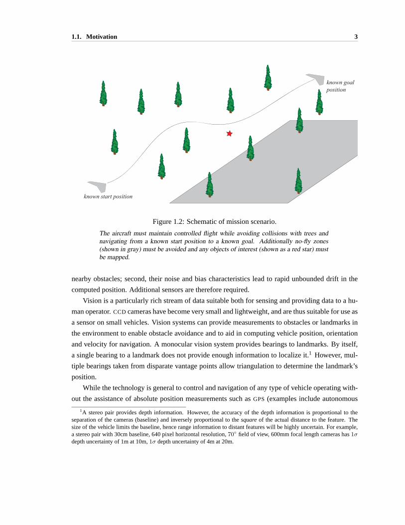
Figure 1.2: Schematic of mission scenario.
The aircraft must maintain controlled flight while avoiding collisions with trees andnavigating from a known start position to a known goal. Additionally no-fly zones(shown in gray) must be avoided and any objects of interest (shown as a red star) mustbe mapped.
nearby obstacles; second, their noise and bias characteristics lead to rapid unbounded drift in the
computed position. Additional sensors are therefore required.
Vision is a particularly rich stream of data suitable both for sensing and providing data to a hu-
man operator.CCD cameras have become very small and lightweight, and are thus suitable for use as
a sensor on small vehicles. Vision systems can provide measurements to obstacles or landmarks in
the environment to enable obstacle avoidance and to aid in computing vehicle position, orientation
and velocity for navigation. A monocular vision system provides bearings to landmarks. By itself,
a single bearing to a landmark does not provide enough information to localize it.1 However, mul-
tiple bearings taken from disparate vantage points allow triangulation to determine the landmark’s
position.
While the technology is general to control and navigation of any type of vehicle operating with-
out the assistance of absolute position measurements such asGPS (examples include autonomous
1A stereo pair provides depth information. However, the accuracy of the depth information is proportional to theseparation of the cameras (baseline) and inversely proportional to thesquareof the actual distance to the feature. Thesize of the vehicle limits the baseline, hence range information to distant features will be highly uncertain. For example,a stereo pair with 30cm baseline, 640 pixel horizontal resolution,70◦ field of view, 600mm focal length cameras has1σdepth uncertainty of 1m at 10m,1σ depth uncertainty of 4m at 20m.

1.2. A Framework for Integrated Control and Navigation 4
underwater vehicles, unmanned ground vehicles operating in caves, indoors or on Mars), the mo-
tivating mission is exploratory flight of a smallUAV through a previously unsurveyed forest (see
Figure 1.2 for a schematic).
1.2 A Framework for Integrated Control and Navigation
Autonomous flight through a forest is an extremely challenging problem. In general successful
operation of aUAV (in any environment, cluttered or clear) involves three basic tasks:
1. The vehicle must maintain controlled flight while avoiding collisions with obstacles (the ve-
hicle mustaviate). This requires a means to determine the state of the vehicle and to detect
and localize obstacles with enough accuracy that appropriate action can be taken.
2. It must find its way from the starting point to a goal location in a finite amount of time (the
vehicle mustnavigate). This requires a means to localize the vehicle relative to the goal.
3. It must convey information about the environment to a human operator or other robots in the
team (the vehicle mustcommunicate). This requires a means of presenting data in a useful
way to human operators or other robots in the team.
These tasks are complicated by the payload limitations imposed by small vehicles (both mass
and dimensions of the total sensing payload are constrained) and by the environments where the ve-
hicle operates. The unavailability ofGPSin cluttered environments means that direct measurements
of vehicle position are unavailable. Furthermore, the environment is unsurveyed, hence obstacle
positions are initially unknown.
The task ofaviation could be accomplished by flying reactively: the vehicle maintains head-
ing until an obstacle is detected, the vehicle maneuvers to avoid the obstacle and then attempts to
reacquire the desired heading. However, while this reactive flight is adequate for small numbers of
well-spaced obstacles, intuition suggests that the limited field of view of most sensors will cause
this approach to fail in more complex environments with densely packed obstacles. Some means
of accounting for obstacles which are outside of the field of view must be provided to plan safe
maneuvers.
While it is certainly aviating, purely reactive flight can hardly be said to benavigation: without
knowledge of aircraft position there is no guarantee of reaching the goal. Thus in order to navigate
in an obstacle-strewn environment some means of obtaining the position of the vehicle must be
provided.
The ultimate purpose of exploratory flight is tocommunicateknowledge of the environment (i.e.
a map) to a human operator or to other robots in the team. If the map is generated in real time as the
vehicle flies through the environment it can also be used to aid aviation (because obstacle locations
are computed) and navigation (because vehicle position in the map is computed).

1.2. A Framework for Integrated Control and Navigation 5
trajectoryplanner
desired flightcondition
flightcontrol
aircraftdynamics
inertial measurementsairspeedangle of attack
estimatorIMU
vision
stabilized aircraft
φ, θ, ψvehicle position, velocityobstacle positions
Figure 1.3: Framework for a vision/inertial measurement navigation system
A stabilized aircraftis an aircraft that can maintain a desired flight condition. Thismay require measurements such as angular rates, angle of attack, sideslip angle andairspeed. In addition bank and pitch angles are required to stabilize certain longer-period dynamic modes, and more complex functions such as altitude hold require ameasurement of altitude.
A framework which enables aviation, navigation and communication is introduced in Figure 1.3.
It comprises three parts: a trajectory planner; a stabilized aircraft; and an estimator. The trajectory
planner uses knowledge of vehicle position and orientation and of the positions of nearby obstacles
to compute a safe trajectory to the goal. A stabilized aircraft is one that can maintain a desired
flight condition (determined based on the trajectory). This is enabled through measurements of
variables such as angular rate and acceleration. Note that knowledge of other variables (such as
angle of bank to control spiral divergence) may be necessary to maintain controlled flight. Finally
the estimator uses available sensing (in this research, anIMU and a monocular camera) to compute
the data required for flight control and trajectory planning2.
The framework presented in Figure 1.3 can be generalized to other vehicles (such as autonomous
underwater vehicles, orAUVs, and unmanned ground vehicles, orUGVs).
Significant advances in sensing, perception, estimation, planning and control must be realized
before flight in cluttered environments can be successfully performed. Loosely defined, sensing and
perception includes obtaining data about the vehicle and its environment and extracting useful in-
formation from the data. In the context of computer vision, perception is the problem of extracting
relevant features in a stream of images. This is an extremely complex problem, especially in natural
environments. Estimation is the process of extracting information about variables of interest from
measurements that are noisy and may be related to these variables through complex mathematical
2In crewed aircraft the pilot provides the additional information required to maintain controlled flight and acts astrajectory planner. Position knowledge may be provided to the pilot by maps or navigation beacons such asGPS.
1.3. The Estimation Problem 6
models. In this application (flight through a forest), the variables of interest include: vehicle ori-
entation and velocity (to maintain controlled flight); obstacle relative position (to avoid collisions);
and vehicle position (to enable navigation to a goal). Planning involves finding a safe, dynamically
feasible path through the forest to a goal location, and finally control involves both stabilizing the
vehicle and following the path computed by the planning algorithm.
The problem of state estimation is directly tied to enabling a smallUAV to aviate and navigate
through the environment and to communicate its acquired knowledge. Hence, the primary contribu-
tion of this dissertation is an estimator which computes the variables necessary for control, obstacle
avoidance, navigation and mapping. Nonlinearities in the system models (both vehicle kinemat-
ics and the vision model) coupled with potentially large uncertainties in system states make this a
particularly difficult estimation problem. This is further exacerbated by the lack of observability
in the system: a monocular vision system provides only bearings to obstacles, making multiple
measurements from different vantage points necessary to localize it.
1.3 The Estimation Problem
The critical technology described is the design of a recursive estimator which fuses inertial and
vision measurements to determine aircraft states and landmark positions. The estimation problem
is highly nonlinear due to the kinematics of the vehicle and the measurement model. The non-
linearities combined with the lack of observability inherent to the problem (due to bearings-only
measurements to landmarks) and the noise and bias errors inherent to low-costIMUs results in an
estimation problem which can not reliably be solved using standard techniques.
Estimating vehicle state as well as the positions of obstacles or landmarks in the environment
is a Simultaneous Localization and Mapping (SLAM) problem, a field of research which has re-
ceived significant attention by the mobile robotics community in recent years. In a typicalSLAM
implementation the vehicle obtains measurements of ego motion (sometimes calledpropriocep-
tive measurements) and relative measurements (generally range and bearing) to nearby landmarks
(calledexteroceptivemeasurements).
The first paper to define landmark positions as states to be estimated was written by Smith and
Cheeseman [50]. Their implementation of an Extended Kalman Filter (EKF) to estimate vehicle and
landmark states was based on a nonlinear vehicle motion model and the nonlinear range and bearing
measurements to landmarks, and this has become a standard approach forSLAM. Kim [27, 25, 26]
describes anEKF-based implementation on a medium-sizedUAV (10kg payload capacity) using in-
ertial measurements along with range and bearings to landmarks. The difficulties of implementing
SLAM on UAVs include highly nonlinear system dynamics, the limits imposed on landmark observ-
ability by trajectory constraints and the high accelerations and roll rates undergone by the vehicle.

1.3. The Estimation Problem 7
The research presented in this dissertation is concerned withSLAM on a smallUAV operating
in a cluttered environment. Since a monocular camera is the only exteroceptive sensor, range mea-
surements are unavailable. This leads to a more difficult case ofSLAM: the reduced observability
complicates the estimation process. Furthermore, in cluttered, obstacle-strewn environments the
vehicle operates in close proximity to the landmarks used as navigation references, increasing the
sensitivity to uncertainties. In this case the uncertainty in the predicted vehicle state and predicted
landmark positions combined with the nonlinearities inherent to the system often causeEKF-based
approaches to diverge.
The bearings-only exteroceptive measurements also complicate the problems of data associa-
tion (correctly associating a bearing with its corresponding landmark) and landmark initialization
(computing an initial estimate of range given only bearing measurements).
This dissertation presents solutions to three challenges inherent to the estimation problem: pre-
venting estimator divergence, data association, and landmark initialization.
1.3.1 Preventing Estimator Divergence
The first problem addressed is estimator divergence, a well known problem which can affect nonlin-
ear estimators. An Extended Kalman Filter (EKF) approximates the system equations by a first order
Taylor series expansion about the current best estimate. The estimate mean and covariance are then
propagated through the linearized system equations. This has proven to be an extremely powerful
technique but there are situations where assumptions inherent to theEKF are not applicable, causing
divergence of the estimated states.
The linearization step of anEKF inherently assumes that uncertainty is small (i.e. it assumes
that the system equations are well approximated by a first order Taylor series expansion over the
span of the uncertainty). If this assumption is invalid there are two effects: first the estimate mean
and covariance may be propagated incorrectly; and second is the (unmodeled) error introduced by
linearizing about the best estimate of the state and not about true state.
When vehicles operate in cluttered environments they are in close proximity to the landmarks
used as navigation references. Because of nonlinearities in the system equations, this close prox-
imity increases the sensitivity of the estimation process to uncertainties. As a result, the estimation
problem described in this dissertation cannot reliably be solved using anEKF because of this in-
creased sensitivity to uncertainties.
This dissertation presents an implementation ofSLAM using an Unscented Kalman Filter (UKF).
The UKF implementation is shown to generate consistent estimates of vehicle state and obstacle
positions, enabling navigation in a cluttered environment without aids such asGPS.

1.3. The Estimation Problem 8
x1
x2 x3
x4
zazb zc
zd
image plane
Figure 1.4: Schematic of data association problem.
Data association is the process of associating measurements {za zb zc zd} with land-marks {x1 x2 x3 x4}.
1.3.2 Data Association
Inherent in any Kalman filter is an assumption of known data association. However, in manySLAM
implementations landmarks are indistinguishable from one another, hence this must be computed
explicitly (see Figure 1.4). It consists of associating measurements{za zb zc zd} with landmarks
{x1 x2 x3 x4}.Data association must be robust to losses of individual features (which may be due to occlusions
or may occur when a landmark is on the edge of the sensor’s detection envelope) and losses of an
entire measurement cycle. It is particularly difficult here because of the small size of the measure-
ment subspace (the 2D image plane as opposed to the 3D physical space). It is especially difficult
when landmarks have not yet been localized to a high degree of accuracy.
In Chapter 3 this dissertation proposes a two stage process for data association: first, the current
bearings are compared with those obtained in a previous frame to check frame to frame correspon-
dence; second, bearings to features not seen in the previous frame are compared with predicted
bearings obtained from landmarks in the map to check if the features have been seen earlier in
the run. Those bearings that are not associated in either step are assumed to come from a new,
previously unseen landmark.
1.3.3 Landmark Initialization
The third problem is landmark initialization, a critical component ofSLAM. It consists of computing
an initial estimate of range given only the measurements to a landmark. In this research it is compli-
cated by the lack of information provided by a single bearing (see Figure 1.5). When a landmark is
initialized its position and covariance must be close enough to truth that the filter does not diverge.

1.3. The Estimation Problem 9
Figure 1.5: Schematic of landmark initialization.
Landmark initialization consists of computing an initial estimate of range given onlybearings to a landmark.
In this dissertation landmarks are assumed to lie on a flat ground plane. Using the estimate
of vehicle altitude a new landmark is initialized at the intersection of the bearing to the landmark
and the ground plane. This can be generalized to non-planar ground with the addition of a digital
elevation map (DEM): landmarks can be initialized at the intersection of the bearing to the feature
and the ground as defined by theDEM.
1.3.4 Additional Issues
Two additional issues inherent to the estimation problem considered here are drift of the estimate
and the effect of vehicle trajectory on the estimate.
Drift
Bearing measurements provide no information about vehicle absolute position or about landmark
absolute position. Absolute position is therefore unobservable, and unless additional information
in the form of absolute measurements are available the estimates of vehicle and landmark absolute
position will drift. If there are no unmodeled dynamics or biases this drift can be modeled as a
random walk.
In most SLAM implementations (including this one) the uncertainty in all the states becomes
highly correlated over the course of vehicle motion. Hence additional information about any of
the states can be used to improve the estimates of all the states. This information may come from
many sources: loop closure, which consists of revisiting previously explored terrain; observation of
a priori known landmarks; or sporadicGPSupdates. With this additional information a smoothing
algorithm can correct the drift in absolute vehicle and landmark positions. Using loop closure to
limit error growth is a standard technique inSLAM.

1.4. Related Work 10
Trajectory Considerations
Since only bearings to obstacles are available, the motion of the camera (i.e. the trajectory flown by
theUAV ) greatly affects the utility of the information gained by subsequent bearing measurements.
During motion directly towards or away from an object (along the bearing) there is no new infor-
mation which improves range estimate. Transverse motion is required to produce a useful estimate
of object position. In the case of obstacle avoidance, transverse motion has the added benefit of en-
suring that a collision is avoided, but the presence of multiple obstacles places conflicting demands
on the trajectory which must be flown.
The choice of trajectory can therefore have a significant effect on the uncertainty associated with
the state estimate. This suggests that trajectories which optimize parameters such as uncertainty in
vehicle position estimate can be designed in addition to the “standard” considerations of obstacle
avoidance or minimum time to reach the goal.
1.4 Related Work
There has been a tremendous amount of research relating to the problem of navigation and state
estimation for mobile robots (flight, ground and undersea). The previous section presented some
references specifically related to aUAV basedSLAM implementation, this section presents a more
detailed discussion of research in the related fields of vision based navigation,SLAM, and Sigma
Point Kalman Filters.
1.4.1 Vision Based Navigation and Structure from Motion
Vision has been extensively studied for use as a sensor in estimation related applications. However
past work has not dealt with estimating all the states necessary for flight in cluttered environments
(i.e. vehicle state and obstacle states). Examples include structure from motion, vision augmented
inertial navigation, real time benthic navigation and relative position estimation.
Structure from motion attempts to reconstruct the trajectory of the video camera and an un-
known scene. An example of an application is given in [42], which describes reconstruction of
archaeological sites using video from a hand-carried camera. However, structure from motion al-
gorithms are typically formulated as batch processes, analyzing and processing all images in the
sequence simultaneously. While this will give the greatest accuracy of both the reconstructed scene
and camera path, it does not lend itself to real-time operation.
Research into vision augmented inertial navigation [47, 31, 37] is primarily concerned with es-
timating the vehicle state by fusing inertial measurements either with bearings to known fiducials or
data from optical flow algorithms. A variant is presented by Diel [11], who uses epipolar constraints
for vision-aided inertial navigation. Positions of unknown obstacles are not estimated.

1.4. Related Work 11
Real time benthic navigation using vision as the primary sensor is described in Marks [32].
Distance from a planar surface (i.e. the ocean floor or a canyon wall) is obtained using a sonar
proximity sensor and texture correlation is used to determine position offsets relative to a reference
image. This capability has been adapted to enable underwater station keeping [29] and has been
extended to incorporate additional sensors [45]. However this technique only estimates vehicle
position, not the position of obstacles in the environment.
Huster [18] demonstrated fusion of inertial and monocular vision measurements for an under-
water object retrieval task. In this case only one object in the environment was considered and
relative position estimation (between the vehicle and object) was performed, not absolute vehicle
and obstacle position estimation.
The use of vision for aidingUAV navigation has become an active area of research. In many
cases vision is not the primary navigation/control sensor but is used in conjunction with inertial
navigation systems andGPS to increase situation awareness. For example, Amidi [1] describes
vision aided navigation for an autonomous helicopter where a stereo pair is used to aid in station
keeping. Sinopoli [49] describe a system that uses data from fusedGPS/INS and a digital elevation
map to plan coarse trajectories which are then refined using data from a vision system. Roberts [46]
describes a flight control system for a helicopter that uses a stereo pair to determine altitude and
optical flow to determine ground speed. Vision aided landing on a pad of known size and shape is
described in [48]. A more complex system for identifying suitable terrain for landing an autonomous
helicopter is described in [33], which uses fusedGPS/INS for control and navigation and a stereo
pair for determining local terrain characteristics.
Vision-based state estimation forUAVs based on techniques derived from structure from motion
are described in [56, 43]. Structure from motion is able to recover scene information and camera
motion up to a scale factor, and an accurate dynamic model of the vehicle is required to help solve
for the scale factor. These techniques are specific to the vehicle carrying the camera, and it is unclear
how external disturbances will affect the result.
Proctor [44] describes a vision-only landing system that performs relative state estimation with
respect to a set of known fiducials. A constant velocity motion model is used to model camera
motion. Wu [58] describes a vision-aided inertial navigation system that relies on measurements to
a known target for vehicle state estimation. Both are examples of terrain aided navigation (TAN),
where measurements to known landmarks are used to aid navigation. Initially unknown environ-
ments are not addressed.
None of the vision aided navigation research described above addresses the problem of simul-
taneously estimating vehicle state and obstacle positions using only monocular vision and inertial
measurements.

1.4. Related Work 12
1.4.2 Simultaneous Localization and Mapping
Simultaneous Localization and Mapping (SLAM, sometimes called Concurrent Mapping and Local-
ization) is the process of simultaneously estimating the state of an autonomous vehicle and land-
marks in the environment. It permits vehicle navigation in an initially unknown environment us-
ing only on-board sensing, and therefore can be used in situations where signals from navigation
beacons such asGPS is unavailable. This dissertation addresses the case of bearings as the only
exteroceptive measurement and a low-costIMU providing proprioceptive measurements for a 6DOF
vehicle operating in close proximity to obstacles.
EKF implementations ofSLAM using range and bearing measurements have been applied both in
simulation and on hardware in many scenarios including indoor navigation of small robots [52], sub-
sea navigation by Autonomous Underwater Vehicles (AUVs) [57] , outdoor navigation by wheeled
robots [30] and navigation by aircraft [25, 26, 27]. In these cases range measurements to landmarks
are available.
Bearings-onlySLAM using cameras mounted on wheeled ground vehicles is described in [28,
15, 35]. In these cases only pure 2D motion is considered and estimation is performed for the planar
environment.
Davison [10] describes a bearings-onlySLAM implementation using only a monocular camera.
Again anEKF is used to recursively estimate the state of the camera and of landmarks, and a constant
velocity model with unknown acceleration is used to describe camera motion. By itself this system
will be able to estimate motion and landmark positions up to a scale factor. To determine the scale
factor the system is initialized by viewing a set of known landmarks. In unexplored environments,
however, there are no known landmarks that can be used to determine the scale and some other
means must be employed.
Burschka [8] describes a fused vision/inertial navigation system for off-road capable vehicles.
Here the main focus is on vehicle pose estimation: a map of the environment is not maintained.
Foxlin [16] describes a wearable vision/inertial system for self-tracking that uses unique coded
fiducials for indoor tracking of humans. A range estimate is computed based on the size of the
fiducial in the image plane.
The research described above does not address the combination of only bearings combined with
inertial measurements, 6DOF estimation for a vehicle flying among obstacles.
1.4.3 Data Association
Typical data association algorithms are based on using aχ2 test to compare an actual measure-
ment with a prediction. After computing likelihoods of possible associations either a gated nearest
neighbor approach is used to determine association on a landmark-by-landmark basis or a joint
compatibility test [36] is used to determine the most likely overall set of associations.

1.4. Related Work 13
Previous work has proposed using additional information (e.g. in an indoorSLAM implementa-
tion described by Neira [35] the lengths of the vertical lines used as features is used as additional
information for data association; Fitzgibbons [15] uses color) to assist in the process of data associ-
ation. In this research additional identifying information is not available: the vision system provides
only a bearing to a landmark.
1.4.4 Landmark Initialization
Methods for feature initialization can be characterized as undelayed or delayed. Undelayed ap-
proaches [10, 19, 28] represent the conical probability distribution function of a single bearing as
a series of Gaussians which are then pruned as more measurements become available. Delayed
methods collect several bearings to a feature from different vehicle poses and compute a landmark
position. It is difficult, however, to obtain an initial landmark position and covariance which is suf-
ficiently Gaussian to prevent divergence of Kalman-type filters. Bailey [2] describes a method for
constrained initialization which computes the “Gaussian-ness” by calculating the Kullback-Leibler
distance. However this is expensive to compute and a threshold value had to be determined experi-
mentally. Another approach is described in Fitzgibbons [15] and in Montesanto [34], where particle
filters are used for landmark placement until the distribution is sufficiently Gaussian to permit a
switch to anEKF framework.
1.4.5 Sigma Point Kalman Filters
Rather than approximating the system equations, particle filters instead approximate thedistribution
of the estimated states with a randomly generated set of points that are propagated through the
full nonlinear system equations [53]. No assumptions regarding the distribution are made and no
assumptions about the characteristics of the noise are made. Therefore they lend themselves very
well to situations where theEKF is not applicable (e.g. due to noise characteristics or the degree
of nonlinearity of the system). However, the number of particles required to adequately model a
distribution is strongly dependent on both the dimension of the state vector and on the uncertainty
of the distribution which is being approximated [53]. Thus in problems with large numbers of states
particle filters quickly become intractable for real-time operation.
Sigma Point Kalman Filters (SP-KF, sometimes called Unscented Kalman Filter, orUKF) can
be viewed as a special case of particle filter that occur when the estimated states and system and
measurement noise obey a Gaussian probability distribution [21, 23, 54]. Rather than a large number
of randomly generated points, a small set of deterministically chosenSigma Pointsare used to
approximate the distribution. The Sigma Points are propagated through the system equations and
then the estimate mean and covariance are recovered. A Sigma Point Kalman Filter is a relatively

1.5. Summary of Contributions 14
new estimation and sensor fusion technique, albeit one that is rapidly gaining acceptance in the
research community.
Variants have been proposed such as the Square Root Unscented Kalman Filter [54], which
propagates the square root of the covariance rather than the covariance itself and a reduced-order
UKF [22], which propagates fewer Sigma Points.
Sigma Point Kalman Filters are being applied to a wide variety of estimation problems. An
SP-KF implementation for integratedGPS/INS navigation is described in [55]. Huster [18] describes
anSP-KF implementation for relative position estimation using a monocular camera andIMU .
1.5 Summary of Contributions
The main contributions of this dissertation are summarized below:
• Framework for Integrated Control and Navigation using only Vision and Inertial sen-
sors
A framework which enables control and navigation of a small autonomous vehicle has been
developed and implemented. This new system fuses data from a low-cost, low powerMEMS
inertial measurement unit and a light-weightCCD camera to reduce drift associated with pure
inertial navigation solutions and to address the technical issues associated with monocular
vision only navigation solutions.
• Estimator Design
An estimator based on the Sigma Point Kalman Filter was developed in the context of this
framework. Vehicle state (position, orientation, velocity),IMU biases and obstacle positions
are estimated. This information was used by a trajectory planner to compute safe paths
through a cluttered environment.
• Performance Verification: Simulation
Results of Monte Carlo simulations ofUAV flight in obstacle-strewn environments show that
the UKF-based implementation provides a solution to the estimation problem. Mean error is
small and the error covariance is accurately predicted. Monte Carlo simulations investigating
error growth characteristics were conducted for two classes of flight: exploration (where new
terrain is being explored) and station keeping (where a set of landmarks may be in continuous
view). For exploration flight the estimated vehicle position estimate error is an approximately
constant percentage of distance traveled, for station keeping flight vehicle position estimate
error varies cyclically with each orbit. For both classes the magnitude of the error varies
inversely with square root of the number of landmarks in view.
• Performance Verification: Hardware
Navigation in a cluttered environment by a small Unmanned Ground Vehicle using only a

1.6. Reader’s Guide 15
low cost IMU and vision sensor was demonstrated. This showed successful state estimation
on an operational system, with real sensor measurements and model and calibration errors.
In addition, the hardware tests demonstrated real-time integration of the estimation algorithm
with an obstacle avoidance and navigation algorithm.
1.6 Reader’s Guide
The remainder of this dissertation is organized as follows:
Chapter 2: The State Estimation Problembegins with a brief discussion of the information
required for flight control, obstacle avoidance and navigation. It then defines the state variables
and develops models for vehicle kinematics, inertial measurements, and vision measurements. It
also includes a discussion of techniques for nonlinear estimation which motivates the application of
a Sigma Point Kalman Filter.
Chapter 3: Estimator Designdescribes the estimation problem, outlining the difficulties associ-
ated with the nonlinearities and uncertainty in this application. It then describes the solution to the
estimation problem.
Chapter 4: UAV Simulation Resultspresents results of Monte Carlo simulations ofUAV flight
in unsurveyed environments. Accuracy of state estimates are addressed through 2D simulations.
Vehicle position estimate error growth characteristics and dependence on the number of landmarks
in view are addressed through 3D simulations.
Chapter 5: Ground Vehicle Results describes a hardware implementation using a small au-
tonomous ground vehicle as test bed. Results of tests demonstrating navigation in an cluttered
environment are presented.
Chapter 6: Conclusionsummarizes results of this research and discusses areas for future work.

Chapter 2
The State Estimation Problem
THIS SECTION DEFINESthe estimation problem introduced in the previous chapter. It has three
purposes: (a) define the state estimation problem; (b) develop equations for plant and sensor
models; (c) provide some justification for applying a Sigma Point Kalman Filter to this estimation
problem. The estimator is then designed and implemented in Chapter 3, and Chapter 4 shows that
theSP-KF-based implementation does indeed result in a convergent, consistent estimator.
The choice of variables used to describe the state of the vehicle and its environment is an im-
portant factor in the design of a solution and its eventual complexity. The state variables must be
sufficient to enable control of the vehicle, avoid obstacles and allow navigation to a goal. At the
same time the choice of state variables has a strong effect on the complexity of the models used to
describe the system. For example, a particular choice of state variables may lead to a very simple
model for the vision system but complex models for vehicle and landmark dynamics. This trade
off must be made in consideration of the limitations imposed by real-time operation of the resulting
estimator.
The equations describing vehicle kinematics, inertial measurements and vision measurements
are highly nonlinear. To provide some intuition into the difficulties associated with nonlinear es-
timation this chapter includes a brief discussion of methods and provides an example comparing
the behavior of three types of nonlinear estimator: the Particle Filter, the Extended Kalman Filter
(EKF), and the Sigma Point Kalman Filter (SP-KF). This motivates the application of a Sigma Point
Kalman Filter to solve the estimation problem.
Section 2.1 defines the estimation problem and state variables. Section 2.2 derives models for
vehicle kinematics, inertial sensors and vision sensors. Section 2.3 discusses three techniques for
nonlinear estimation (Particle Filter,EKF andSP-KF). Finally Section 2.4 provides a summary.
16

2.1. Problem Statement 17
Figure 2.1: Schematic of estimation problem.
The aircraft obtains bearings to fixed landmarks (tree trunks) and measurements of ac-celeration and angular rate. Using these measurements an estimate of aircraft position,orientation, and velocity as well as obstacle positions must be obtained.
2.1 Problem Statement
As discussed in Chapter 1 the scenario considered here consists of a smallUAV flying through an
unsurveyed forest (Figure 2.1) using only an inertial measurement unit and a monocular camera.
The on-board camera obtains bearing measurements to obstacles (tree trunks) and the inertial mea-
surement unit provides accelerations and angular rates in the body-fixed frame.
For the purpose of this dissertation, flight control is taken to refer only to the maintenance of
steady, controlled flight (the first part of theaviate task: the second part is obstacle avoidance).
Navigation refers to directed motion towards a goal. In general the information required for flight
control differs from that required for navigation, and often the computations and actions required
for flight control occur at much higher rate than those for navigation. Flight control systems have
been the subject of enormous amounts of research and have been covered in numerous textbooks
(e.g. Blakelock [4], Bryson [7], or Etkin [13]). In general angular rate, orientation and speed are
required for flight control (see Appendix A for an illustrative example), vehicle position is required
for navigation and obstacle relative position is required for obstacle avoidance. This is summarized
in Table 2.1.
In addition to vehicle position, orientation and speed, low costIMUs are subject to scale factor
and bias errors that can drift with time, thus estimates of scale factor and bias are also required. The
vehicle state vector is
xv =[x y z φ θ ψ u v w αT bTa bTω
]T(2.1)

2.1. Problem Statement 18
Table 2.1: Required information.
description purpose source
angular rate flight control measured byIMU
orientation flight control and navigation estimatedspeed flight control and navigation estimated
vehicle position navigation estimatedobstacle relative position collision avoidance estimated
Referring to Figure 2.1, (x y z) represents position in the inertial frame, (φ θ ψ) represent Euler
angles with respect to the inertial frame, (u v w) represents velocity expressed in the body frame,
αT representsIMU scale factor error,bTa represents accelerometer bias, and finallybTω represents
rate gyro bias.
In addition to vehicle state, obstacle relative positions are required. In this dissertation absolute
obstacle positions in the inertial frame are estimated. This simplifies the mapping process and, as
will be further discussed in Chapter 3, simplifies the computational requirements of the resulting
estimator. Obstacle relative position can easily be computed from the absolute obstacle position and
vehicle absolute position.
The final state vector is
x =[
xTv xT1 xT2 · · · xTm]T
(2.2)
wherexv is the vehicle state defined in Equation 2.1 andxi = [xi yi zi]T , the position of theith
obstacle in the inertial frame.
Given the noisy, limited measurements available from theIMU and vision system, the problem
is to obtain the information required to control the aircraft, avoid collisions with obstacles and to
permit navigation. That is, the problem is to compute an estimatex and covarianceP of the state
vectorx given a process model
x = f(x,u) (2.3)
and a measurement model
zimu = g1(x,u) (2.4)
zcam = g2(x) (2.5)
Hereu represent inputs to the plant,zimu represent inertial measurements, andzcam represents
bearing measurements. The process modelf is developed in Section 2.2.2, the inertial measurement
model g1 is developed in Section 2.2.3 and the vision modelg2 is developed in Section 2.2.4.
Chapter 3 integrates the models to form the prediction equations and the vision update equations. A

2.2. Sensor and System Models 19
Figure 2.2: Coordinate frames.
Frame O is an inertial NED frame. B is the vehicle body-fixed frame, the matrix Tdefines the transformation of a vector in O to its representation in B. Frame C is thecamera-fixed frame, with the camera’s optical axis aligned with xc. The transformationTcam between the camera frame and the body frame B is assumed known and theaxes of the inertial measurement unit are assumed to be aligned perfectly with the bodyframe B.
complete summary of the equations used in the estimator prediction and correction steps is given in
Appendix B.
2.2 Sensor and System Models
2.2.1 Coordinate Frames
Navigation is done with respect to an inertial North-East-Down (NED) coordinate frameO. Sensors
are fixed to the vehicle with known position and angular offsets with respect to a body-fixed frame
B. Acceleration and angular rate are measured using a strapdown inertial measurement unit in the
body frameB, bearings to landmarks are obtained in a camera frameC. Transformation matrices
T andTcam define the transformation of a vector expressed inO toB and a vector expressed inB
toC, respectively. Coordinate frames are shown schematically in Figure 2.2.
2.2.2 Vehicle Kinematic Model
A dynamic model requires knowledge of all inputs, including disturbances. For smallUAVs there
is a very high degree of uncertainty associated with disturbances which act on the vehicle1. In this
1Disturbances would consist of gusts, which are extremely difficult to characterize in cluttered environments.

2.2. Sensor and System Models 20
case a standard technique is to use a kinematic model driven by inertial measurements as a process
model.
Vehicle positionx, y, z is expressed in the inertial frame, rotations are expressed as Euler angles
φ, θ, ψ relative to the inertial frame and velocityu, v, w are in expressed in the body frame. The
coordinate transformT (defined in Equation 2.11) projects a vector expressed in the inertial frame
O into the body frameB. Vehicle kinematics are: x
y
z
= T−1
u
v
w
(2.6)
The transformation matrixT is defined by the Euler angles of the aircraft with respect to the
inertial frame. Following a roll-pitch-yaw convention,
T = TφTθTψ (2.7)
where
Tφ =
1 0 00 cosφ sinφ0 − sinφ cosφ
(2.8)
Tθ =
cos θ 0 − sin θ0 1 0
sin θ 0 cos θ
(2.9)
Tψ =
cosψ sinψ 0− sinψ cosψ 0
0 0 1
(2.10)
Therefore,
T =
cos θ cosψ cos θ sinψ − sin θsinφ sin θ cosψ − cosφ sinψ sinφ sin θ sinψ + cosφ cosψ sinφ cos θcosφ sin θ cosψ + sinφ sinψ cosφ sin θ sinψ − sinφ cosψ cosφ cos θ
(2.11)
Body angular rates can be expressed as Euler angle rates by: φ
θ
ψ
=
1 sinφ tan θ cosφ tan θ0 cosφ − sinφ0 sinφ
cos θcosφcos θ
p
q
r
(2.12)
2.2. Sensor and System Models 21
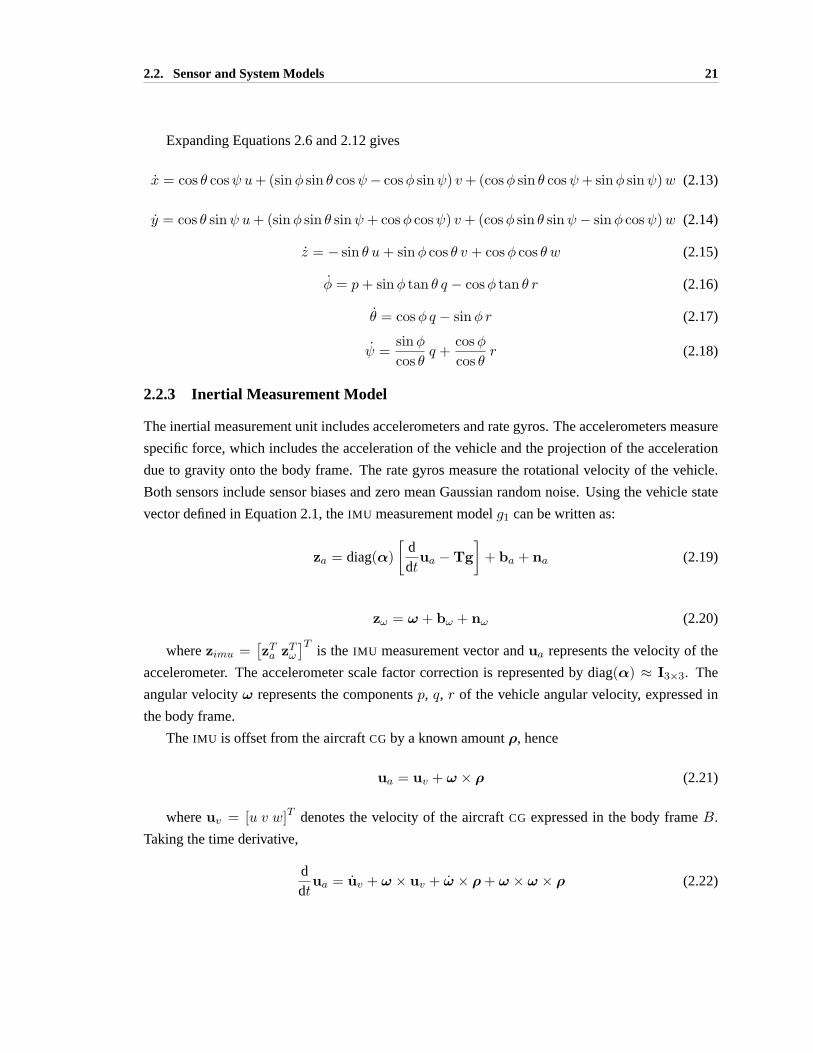
Expanding Equations 2.6 and 2.12 gives
x = cos θ cosψ u+ (sinφ sin θ cosψ− cosφ sinψ) v+ (cosφ sin θ cosψ+ sinφ sinψ)w (2.13)
y = cos θ sinψ u+ (sinφ sin θ sinψ+ cosφ cosψ) v+ (cosφ sin θ sinψ− sinφ cosψ)w (2.14)
z = − sin θ u+ sinφ cos θ v + cosφ cos θ w (2.15)
φ = p+ sinφ tan θ q − cosφ tan θ r (2.16)
θ = cosφ q − sinφ r (2.17)
ψ =sinφcos θ
q +cosφcos θ
r (2.18)
2.2.3 Inertial Measurement Model
The inertial measurement unit includes accelerometers and rate gyros. The accelerometers measure
specific force, which includes the acceleration of the vehicle and the projection of the acceleration
due to gravity onto the body frame. The rate gyros measure the rotational velocity of the vehicle.
Both sensors include sensor biases and zero mean Gaussian random noise. Using the vehicle state
vector defined in Equation 2.1, theIMU measurement modelg1 can be written as:
za = diag(α)[
ddt
ua −Tg]
+ ba + na (2.19)
zω = ω + bω + nω (2.20)
wherezimu =[zTa zTω
]Tis the IMU measurement vector andua represents the velocity of the
accelerometer. The accelerometer scale factor correction is represented by diag(α) ≈ I3×3. The
angular velocityω represents the componentsp, q, r of the vehicle angular velocity, expressed in
the body frame.
The IMU is offset from the aircraftCG by a known amountρ, hence
ua = uv + ω × ρ (2.21)
whereuv = [u v w]T denotes the velocity of the aircraftCG expressed in the body frameB.
Taking the time derivative,
ddt
ua = uv + ω × uv + ω × ρ + ω × ω × ρ (2.22)

2.2. Sensor and System Models 22
The terms containingρ can be collected into a single expression representing the accelerations
induced by the offset of theIMU from the aircraftCG:
ddt
ua = uv + ω × uv + b(ρ) (2.23)
Finally the accelerometer measurement model can be written as:
za = diag(α) [uv + ω × uv + b(ρ)−Tg] + ba + na (2.24)
Sensor biases and the accelerometer scale factor are assumed to vary by a random walk model
with zero mean Gaussian driving terms.
α = nα (2.25)
ba = nba (2.26)
bω = nbω (2.27)
i.e. n(·) ∼ N (0,Σ(·)).
2.2.4 Vision Model
The camera is assumed to be fixed to the aircraft with known offset4s from the CG and known
angular offset from the body-fixed frame, defined by a transformationTcam. The camerax-axis is
perpendicular to the image plane (coordinate frames are defined in Figure 2.2).
A pinhole camera model (Figure 2.3) describes the projection of a vector onto the image plane
as
z =f
x
[y
z
](2.28)
wheref is the focal length and[x y z]T is the vector (expressed in the camera frame). The focal
lengthf can be normalized without loss of generality.
For cameras with “standard” field of view (less than approximately70◦) this model is sufficient.
In wide field of view cameras (& 90◦) this model becomes problematic. The pinhole projection
model becomes ill-conditioned for vectors which are close to90◦ away from the optical axis (the
componentx of the vector expressed in the camera frame approaches 0). To improve conditioning
and to express bearings as azimuth and depression (in the coordinate frames used here a positive
angle is down with respect to the optical axis) measurements are modeled as arctangents of the
projection onto the image plane (Figure 2.3). For theith landmark the vision measurement model
g2,i is:
zcam,i =
[arctan si,y
si,x
arctan si,z
si,x
]+ nc (2.29)

2.3. Nonlinear Estimation 23
x
yz
s
image plane
siz
siy
(a) Pinhole model.
x
yz
s
image plane
γyγz
(b) Modified pinhole model.
Figure 2.3: Projection models.
Rather than express the pinhole projection as vector components in the image plane(left image), the projection is expressed as an azimuth and depression to the feature(right image). This leads to better conditioning of the measurement model.
The measurement is corrupted by zero-mean Gaussian noisenc. si represents the vector from
the camera to theith tree, expressed in the camera frame:
si = Tcam
T
xi − x
yi − y
zi − z
−4s
(2.30)
When vision measurements to several landmarks are available the vision measurement vector is
formed by concatenating the available measurements, i.e.zcam =[zTcam,1 zTcam,2 . . . zTcam,m
]T.
2.3 Nonlinear Estimation
In general estimators follow a recursive process of prediction (governed by a plant model) followed
by correction (governed by a measurement model). The equations describing vehicle kinematics
and the available measurements are highly nonlinear. In addition, the uncertainty in estimated states
is likely to be significant due to the noise characteristics of low-costIMUs. The combination of sig-
nificant nonlinearities and large uncertainty greatly complicates the state estimation problem. This
section briefly discusses and compares three techniques for nonlinear estimation: the Particle Filter,
the Extended Kalman Filter and the Sigma Point Kalman Filter (sometimes called the Unscented
Kalman Filter). Its purpose is to motivate the application of aSP-KF to an estimation problem with
the types of nonlinearities as those seen in this research (i.e. trigonometric functions).

2.3. Nonlinear Estimation 24
For linear systems subject to Gaussian noise and whose state variables can be accurately de-
scribed with Gaussian probability distribution functions the Kalman Filter is the optimal solution
to the estimation problem. The Kalman Filter has been extensively described in the literature, and
textbooks such as Kailath [24] provide in-depth derivations.
However, optimal solutions to nonlinear estimation problems have proven to be difficult to ob-
tain. In most cases approximations are required, and these approximations greatly reduce any claims
of optimality or in some cases even convergence. These approximations can be categorized into
probability distribution approximationsor system approximations. For example, Particle Filters ap-
proximate the distribution with a large group of particles, Extended Kalman Filters approximate the
system with a linearization.
It is often assumed that random variables obey a Gaussian probability distribution. In Kalman
filters it is further assumed that the probability distribution remains Gaussian after propagation
through the system equations (for linear systems this is true). For nonlinear functions that have
extrema (for example trigonometric functions such assin θ) the assumption of preservation of
Gaussian-ness is false at the extrema.
Trigonometric functions appear in coordinate transformations in both the inertial measurement
model described in Section 2.3.3 and the vision model described in Section 2.3.4. The remainder
of this section uses the functionf(θ) = − sin θ as an example to illustrate the propagation of a
Gaussian random variableθ ∼ N (θ, σθ) through a trigonometric function using a Particle Filter,
linearization (as would occur in anEKF) and a sigma point transform (as would occur in aSP-KF).
The effect of assuming thatf(θ) is Gaussian and of linearization ofsin θ will be illustrated.
These techniques are then compared in a single time-update step for a planar non-holonomic
vehicle, a simplified model of the aircraft kinematic model used in this research.
2.3.1 Particle Filters
A particle filter represents a probability distribution as a family of particles sampled randomly from
the desired probability distribution function (PDF). In principle anyPDF can be modeled, avoiding
the necessity of assuming a specificPDF. In addition noise can have an arbitraryPDF.
In the prediction step the particles are propagated through the nonlinear process equations.
When measurements are available each particle is assigned a weight based on how closely the
measurement prediction for that particle matches the actual measurement (i.e. a close match means
the particle is likely to represent the true system state). These weights are then used to resample the
family of particles: those with high weight are likely to be selected for continued propagation, those
with low weight are not likely to be selected.
The accuracy of the particle filter is directly related to the number of particles used to represent
the PDF. In principle it becomes arbitrarily accurate as the number of particles is increased (in
practice there are still some issues being researched) at the cost of increased computation. For

2.3. Nonlinear Estimation 25
0 90 180 270 3600
0.2
0.4
0.6
0.8
1
1.2
θ (degrees), P(sin(θ)
sin(
θ)
Figure 2.4: Particle representing a Gaussian PDF propagated through sine function.
The black solid line represents − sin θ, the dotted green “bell” represents a histogramof a Gaussian PDF with mean 265◦ and standard deviation 10◦ (scaled to fit plot). Thedotted green curve along the vertical axis represents a histogram of the Gaussian PDF
propagated through f(θ) = − sin θ (scaled to fit plot). The solid green “bell” representsa Gaussian PDF with the same mean and standard deviation as the PDF of − sin θ.
systems with many states the number of particles required to adequately model thePDF generally
precludes real time implementation, but they serve as a useful benchmark by which theEKF and
SP-KF can be judged.
Figure 2.4 shows the propagation of a GaussianPDF θ ∼ N (265◦, 10◦) through the function
f(θ) = − sin θ using a particle representation with106 particles. Note that the resulting distribution
is not Gaussian, and that a Gaussian approximation to the resultingPDF is not particularly accurate.
However, for values ofθ sufficiently far from the extrema off (i.e. several standard deviations) the
assumption of Gaussian-ness off(θ) will be approximately true.
The assumption that GaussianPDFs remain Gaussian after propagation through the system equa-
tions is in common practice and in most cases performance of the resulting estimators is good.
2.3.2 Extended Kalman Filter
An Extended Kalman Filter approximates nonlinear system models with a first-order Taylor se-
ries approximation about the current best estimate. This linearization introduces errors in several
ways: first, a potentially highly nonlinear system is approximated with a linear model; second, the
linearization occurs about an uncertain state, hence the linearization itself may be incorrect. In esti-
mation problems the linearization error becomes problematic when the system cannot be accurately
approximated by a first order Taylor series over the span of uncertainty in the states.

2.3. Nonlinear Estimation 26
0 90 180 270 3600
0.2
0.4
0.6
0.8
1
1.2
θ (degrees), P(sin(θ)
sin(
θ)
Figure 2.5: Linearized propagation of random variable through sine function
The black solid line represents − sin θ, the dotted green “bell” represents a histogramof a Gaussian PDF with mean 265◦ and standard deviation 10◦ (scaled to fit plot). Thestraight red line denotes the linearization of f(θ) = − sin θ at 265◦. The solid red “bell”represents the mapping of θ ∼ N (265◦, 10◦) through the linearization of − sin θ. Forcomparison, the solid green “bell” is the Gaussian approximation of the particle filter.
Figure 2.5 shows the propagation ofθ ∼ N (265◦, 10◦) through the linearized model of the
functionf(θ) = − sin θ. In comparison with the Gaussian approximation of the particle filter, the
system linearization shows both a bias in the mean and smaller uncertainty. This bias and smaller
uncertainty will be exacerbated both asθ approaches the extrema of the sine function and as the
uncertainty inθ is increased.
This indicates that in some cases linearization of the system equations results in both a bias and
an artificial increase in the certainty associated with an estimate.
2.3.3 Sigma Point Filters
Rather than approximate the nonlinear system equations, anUKF [23] [55] instead approximates
the probability distribution of the state which is to be estimated. In contrast with a particle filter,
which makes no assumption about thePDF, Sigma Point Filters assume a GaussianPDF of the
state variables, which allows a greatly reduced set of particles to model thePDF. The probability
distribution is represented by a set ofSigma Pointswhich capture the mean and covariance of a
random vectorx = N (x,P):
X =[
x x + η√
P x− η√
P]
(2.31)

2.3. Nonlinear Estimation 27
0 90 180 270 3600
0.2
0.4
0.6
0.8
1
1.2
θ (degrees), P(sin(θ)
sin(
θ)
Figure 2.6: Unscented transform
The black solid line represents − sin θ, the dotted green “bell” represents a histogramof a Gaussian PDF with mean 265◦ and standard deviation 10◦ (scaled to fit plot). Thethree blue dots on the bell denote the three Sigma points which represent θ. The solidblue bell on the vertical axis denotes the PDF recovered from the propagated Sigmapoints. It almost exactly covers the solid green “bell” representing the Gaussian ap-proximation of the particle filter.
Hereη is a scale factor and√
P is an orthogonal matrix square root of the covariance of the
distribution2. These Sigma Points are propagated through the full nonlinear system equations and
the estimate mean and covariance are then recovered.
Figure 2.6 shows the propagation ofθ ∼ N (265◦, 10◦) through− sin θ using three Sigma
points. With only three Sigma points the Gaussian approximation of the particle filter is captured
almost exactly.
Sigma point Kalman filters follow the familiar pattern of prediction followed by correction. The
algorithm in [54] is reproduced in Figure 2.7.
2.3.4 Comparison of Techniques
The effect of both the assumption of preservation of Gaussian-ness and theEKF’s linearization error
can be seen using a single prediction step for the motion of a 2D non-holonomic vehicle (a simplified
2Note that this matrix square root is not unique: it can be chosen based on issues such as numerical stability, com-putational cost or to exploit known structure in the problem (Huster [18] makes use of this property: he chooses sigmapoints so that the range to the target is always positive).

2.3. Nonlinear Estimation 28
initialize with x0 andP0|0.
For tk, k ∈ (1, . . . ,∞) compute sigma points:
Xk−1|k−1 =[
xk−1|k−1 xk−1|k−1 + η√
Pk−1|k−1 xk−1|k−1 + η√
Pk−1|k−1
](2.32)
Time update (prediction):Xk|k−1 = f(Xk−1|k−1,uk−1) (2.33)
xk|k−1 = Xk|k−1wm (2.34)
Pk|k−1 =[Xk|k−1 − xk|k−11
]T Wc
[Xk|k−1 − xk|k−11
]+ Q (2.35)
Measurement update (correction):
Zk|k−1 = h(Xk|k−1) (2.36)
zk|k−1 = Zk|k−1wm (2.37)
Pzz =[Zk|k−1 − zk|k−11
]T Wc
[Zk|k−1 − zk|k−11
]+ R (2.38)
Pxz =[Xk|k−1 − xk|k−11
]T Wc
[Zk|k−1 − zk|k−11
](2.39)
K = PxzP−1zz (2.40)
xk|k = xk|k−1 + K(zk − zk|k−1) (2.41)
Pk|k = Pk|k−1 −KPzzKT (2.42)
There are2N + 1 sigma points, whereN is the dimension of the state vector. In this algorithmη is a weight factor,wm is a vector of weights,Wc is a diagonal matrix of weights,1 is a(1 × 2N + 1) matrix of ones,Q is process noise andR is measurement noise. The weightfactors are calculated as
η = α√N (2.43)
The constantα is a parameter which determines the spread of the sigma points. Typically10−4 ≤ α ≤ 1. The weight vectorwm and weight matrixWc are
wm,1 = α2−1α2 wm,i = 1
2Nα2 (2.44)
Wc,1 = α2−1α2 + (1− α2 + β) Wc,ii = 1
2Nα2 (2.45)
wherei = 2, . . . , (2N + 1). The parameterβ incorporates prior knowledge of the distributionof the state vector. For Gaussian distributionsβ = 2 is optimal [54].
Figure 2.7: Algorithm for Unscented Kalman Filter.
reproduced from Rudolph van der Merwe and Eric Wan, ”The Square Root UnscentedKalman Filter for State and Parameter Estimation”, IEEE International Conference onAcoustics, Speech and Signal Processing, Salt Lake City, UT, 2001.

2.3. Nonlinear Estimation 29
−5 0 5 10 15 20−5
0
5
x
yParticlesEKFparticle filterUKF
Figure 2.8: Single time update for non-holonomic vehicle.
Nominal initial vehicle position is at the origin, aligned with x axis. Initial uncertaintyis 1cm in position and 10◦ in heading. Black dots show particles propagated throughmotion equations, solid green ellipsoid shows 3σ uncertainty of Gaussian approxima-tion of particles. Dashed red ellipsoid shows EKF computation of motion, dotted blueellipsoid shows Sigma Point computation of motion.
model of the aircraft kinematics used in this dissertation). Vehicle motion is modeled as xk+1
yk+1
ψk+1
=
xk + u∆t cosψyk + u∆t sinψψk + ψ∆t
(2.46)
It is assumed that perfect odometry is available (i.e.u∆t = 10 and ψ∆t = 0 are known
precisely).
Figure 2.8 shows a single time-update step for a particle filter, a Gaussian approximation to the
particle filter, anEKF, and aSP-KF. The vehicle begins at the origin with initial position uncertainty
of 1cm and initial heading uncertainty of10◦. The particle filter results show the distinct ‘banana’
shape of thePDF of the predicted vehicle position. Ellipses show3σ uncertainty for the Gaussian
approximation (solid green),EKF (dashed red), andSP-KF (dotted blue).
The propagation of the mean and covariance through the linearized equations of theEKF in-
troduces a bias in the vehicle position and causes the uncertainty in vehicle position (i.e. the co-
variance) to be significantly under predicted. TheSP-KF comes significantly closer to the Gaussian
approximation, almost exactly computing the mean and slightly over predicting the uncertainty. The
computation cost of theSP-KF is similar to theEKF solution.
Another, more detailed, comparison of estimation techniques applied to a bearings-only track-
ing problem is provided by Huster [18]. That comparison shows that theEKF fails to compute a

2.4. Summary: The Estimation Problem 30
converged estimate of system state, while theSP-KF implementation computes an estimate almost
identical to a particle filter implementation.
2.4 Summary: The Estimation Problem
To operate successfully in cluttered environment theUAV must maintain controlled flight, avoid
collisions with obstacles and navigate to a goal location. This requires knowledge of vehicle ori-
entation and speed, obstacle relative position and vehicle position. This must be computed using
information provided by theIMU (i.e. noisy, biased measurements of acceleration and angular rate)
and the vision system (noisy measurements of bearings to obstacles). Because of the possibility of
drift, IMU biases must also be computed.
This can be performed with a recursive estimator which computes an estimate of system state
(i.e. the vehicle state as defined in Equation 2.1 and obstacle positions) and the associated covari-
ance:
x =
[xvxo
](2.47)
P =
[Pvv Pvo
Pov Poo
](2.48)
Because of the high degree of uncertainty associated with the disturbances acting on a small
UAV a kinematic model driven by inertial measurements is used as the plant model. The use of
an inertial-measurement driven kinematic model means that the same sensor package and estimator
can, in principle, be used with different classes of vehicle (for example autonomous ground vehicles
or underwater vehicles).
Both the inertial measurement model and the vision model are highly nonlinear. Vehicle ori-
entation (expressed as Euler angles) accounts for nonlinearities in both the inertial model and the
vision model due to the transformations of vectors between coordinate frames. The modified pin-
hole model which projects the three-dimensional world onto the camera’s two dimensional image
plane causes further nonlinearities in the vision model.
The linearized system equations used by theEKF causes a bias in the propagated mean of a
GaussianPDF and computes a decreased propagated covariance. This suggests thatEKF-based
estimators are likely to fail when trigonometric functions are a significant source of nonlinearities
in the system equations.
In contrast, the mean and covariance of a GaussianPDF propagated through the nonlinear equa-
tions using Sigma Points accurately models the true mean and covariance. This suggests that a
SP-KF is a good candidate for solving estimation problems which contain trigonometric functions.

2.4. Summary: The Estimation Problem 31
A solution of the estimation problem using theSP-KF is given in Chapter 3 and simulation results
presented in Chapter 4 verify the consistency of the estimator.

Chapter 3
Estimator Design
THIS CHAPTER DESCRIBESin detail the inertial/vision navigation filter developed in this re-
search. The process of computing vehicle state and obstacle positions using inertial measure-
ments and bearings is a Simultaneous Localization and Mapping (SLAM) problem. It is complicated
by three factors: the nonlinearities in the system and measurement models (described in Chapter 2);
the lack of observability inherent to the bearings-only measurements provided by the vision sys-
tem; and by the significant uncertainty in state estimates. This chapter presents: (a) a Sigma Point
Kalman Filter based implementation to solve the estimation problem; (b) a solution to the problem
of data association; (c) a solution to the problem of landmark initialization; and (d) a method to
incorporate absolute position measurements which may occasionally be available.
Using the system models derived in the previous chapter, aSP-KF is implemented in Section 3.1.
The SP-KF is able to cope with the system nonlinearities while being tractable for real-time opera-
tion.
Data association must be computed explicitly. A two step approach is described in Section 3.2,
where the first step seeks to associate features observed in the current image frame with those
observed in the previous frame and the second step associates features in the current image frame
with predictions obtained from the current map.
Section 3.3 describes a method for landmark initialization, where a new landmark is initialized
at the intersection of the bearing to a previously unseen landmark and the ground plane.
Estimating vehicle state and obstacle positions using the techniques described here is a stand-
alone process. However, an absolute position measurement may be sporadically available (either
through aGPSmeasurement or because the known goal has been reached). Since errors in estimates
are fully correlated, additional information about any state can be used to improve the estimates of
all states. This is addressed in Section 3.4, which describes a correction step of the map.
Section 3.5 concludes this chapter with a summary of data flow in the full estimation process,
including data association, landmark initialization, and estimate smoothing/correction. Results of
32
3.1. Inertial/Vision Navigation Filter 33
simulations ofUAV flight in cluttered environments are presented in Chapter 4 to demonstrate es-
timator performance, results of hardware and simulation tests using a small Unmanned Ground
Vehicle are presented in Chapter 5.
3.1 Inertial/Vision Navigation Filter
As stated in Chapter 2 the vector of states to be estimated is
x =[
xTv xT1 xT2 · · · xTm]T
(3.1)
wherexi = [xi yi zi]T , the position of an obstacle in the inertial frame and
xv =[x y z φ θ ψ u v w αT bTa bTω
]T(3.2)
The process model
x = f(x,u) (3.3)
and the measurement model
zimu = g1(x,u) (3.4)
zcam = g2(x) (3.5)
were developed in Chapter 2. This section integrates the models to form the prediction equations
and the vision update equations. A summary of the estimator prediction and correction equations is
given in Appendix B.
In general estimators follow a recursive process of prediction followed by correction. In many
cases the prediction step is driven by a dynamic model of the system driven by known inputs and
unknown disturbances, where it is assumed that the disturbances can be adequately modeled by
random process noise. In this dissertation the prediction step is performed by a kinematic model
driven by accelerometer and angular rate measurements. Noise in these measurements is treated as
process noise.
The correction step is driven by the bearing measurements obtained from the vision system.
3.1.1 Prediction Step
Incorporating the rate gyro measurement model (Equation 2.20) into Equations 2.16–2.18 relates
measurements of angular rate to the Euler angle rates:
φ = (zp − bp) + tan θsinφ(zq − bq)− tan θcosφ(zr − br) (3.6)

3.1. Inertial/Vision Navigation Filter 34
θ = cosφ(zq − bq)− sinφ(zr − br) (3.7)
ψ =sinφcos θ
(zq − bq) +cosφcos θ
(zr − br) (3.8)
wherebp, bq, andbr are the rate gyro biases. The vehicle acceleration is obtained from the ac-
celerometer model (Equation 2.24) and the rate gyro model (Equations 2.20):
u =zxαx
− gsin θ − bx − (zq − bq)w + (zr − br)v − bx(ρ) (3.9)
v =zyαy
+ gcos θsinφ− by − (zr − br)u+ (zp − bp)w − by(ρ) (3.10)
w =zzαz
+ gcos θcosφ− bz − (zp − bp)v + (zq − bq)u− bz(ρ) (3.11)
z(·) andb(·) represent the inertial measurement and bias, respectively, along a body-fixed axis.
α(·) is the accelerometer scale factor error along a body-fixed axis,g is the acceleration due to
gravity andb(·)(ρ) is the acceleration induced by the (known) offset of theIMU from the vehicle
CG.
IMU biases vary as a random walk:
α = nα (3.12)
ba = nba (3.13)
bω = nbω (3.14)
whereα = [αx αy αz]T , ba = [bx by bz]
T andbω = [bp bq br]T .
Finally, obstacles are assumed to be stationary, hence
xi = 0 (3.15)
Equations 2.13–2.15, 3.6–3.8, 3.9–3.11 and 3.12–3.15 represent the kinematics of the vehicle,
inertial measurement unit and obstacles. These can be written in compactly in discrete form as[xv,k+1
xo,k+1
]=
[fdv (xv,k, zimu,k)
xo,k
]+
[next0
](3.16)
The nonlinear functionfdv captures the discrete-form kinematics of the vehicle and theIMU bias
states and is driven by the inertial measurementszimu,k. The external noise termnext includes the
assumed noise of the random walk model for theIMU scale factor and bias drift and may include an
additional noise term to cover unmodeled vehicle kinematics. Inertial measurements are assumed
to be corrupted by zero mean Gaussian random noise.

3.1. Inertial/Vision Navigation Filter 35
The system kinematic equations are used in the prediction step of theUKF algorithm reproduced
in Figure 2.7. The process noise for the time update must still be obtained. In this case process noise
arises from the noisy measurements of acceleration and angular rate. Process noise is approximated
as
Qk =
[FzΣimuFTz + Σext 0
0 0
](3.17)
whereFz = ∇zimu fdv (the Jacobian of the discrete process model with respect to the inertial
measurements),Σimu is the covariance matrix describing theIMU measurement noise, andΣext is
the covariance describing the external noise, including drift of theIMU biases. This is identical to
the EKF process noise approximation, and is adequate for the application being considered. Since
obstacles (i.e. trees) are assumed to be perfectly stationary only components corresponding to
vehicle states have non-zero process noise.
Note that measurements from theIMU are likely to be available at a much higher rate than
measurements from the camera, allowing the time update to proceed at a higher rate than the vision
correction.
3.1.2 Vision Update
Measurements from the camera are incorporated in the measurement update step of the estimator.
The vision model reflects the projection of a vector in 3D (the vector from the vehicle to the fea-
ture) onto the 2D image plane and is represented by Equations 2.29 and 2.30. This can be written
compactly as
zcam,k = g2(xv,k,xo,k) + nc (3.18)
Herezcam represents bearings from the vehicle to stationary features. Measurement noise is
represented by the zero-mean Gaussian random variablenc.
3.1.3 Choice of States
Recall from Chapter 2 that only relative obstacle position is required to avoid collision. A different
state vector including vehicle state and range and bearings to obstacles instead of absolute obstacle
position would also provide the information required for control and navigation. Since the vision
system provides a measurement of bearing to obstacles, this would result in a linear vision update
step.
However, while absolute obstacle position is constant, relative position changes continuously
and is a nonlinear function of vehicle motion, resulting in a more complex prediction step. The
prediction step runs at theIMU measurement rate, which is typically much higher than the vision
frame rate. Computationally, estimating obstacle relative position is more expensive than estimating

3.2. Data Association 36
absolute position. Absolute obstacle position estimation has the additional benefit of immediately
providing a map of obstacle positions in the inertial frame.
Hence absolute obstacle position is estimated along with vehicle position, orientation, and ve-
locity.
3.2 Data Association
Inherent in any Kalman filter is an assumption of known data association. However, in this ap-
plication (as in manySLAM implementations) landmarks are indistinguishable from one another1,
hence this must be computed explicitly. In this research it is complicated by the lack of complete
measurements (i.e. bearings provide two measurements, range is not available).
A two stage process is used for data association: first, the current bearings are compared with
those obtained in a previous frame to check frame to frame correspondence; second, bearings to
features not seen in the previous frame are compared with predicted bearings obtained from land-
marks in the map to check if the features have been seen earlier in the run. Those bearings that are
not associated in either step are assumed to come from a new, previously unseen landmark.
Frame to frame association for point features is used extensively in optical flow algorithms. Typ-
ically these operate at high frame rates compared with motion of the vehicle. However, when frame
rates are low and vehicle motion (especially angular motion) is large, frame to frame correlation is
more complex. However, additional information to aid frame to frame association is available.
Angular rate measurements available from theIMU are integrated to obtain the change in ori-
entation of the camera between frames. The change in orientation is used to calculate predicted
bearings for features seen in the previous frame and these are compared with current measurements.
While changes in position of the vehicle will also affect the predicted bearings, this is a much
smaller effect than changes in orientation. Also, changes in bearing to a feature due to changes in
vehicle position require a measurement of range (which is unavailable here) to the feature to com-
pute. Hence bearing changes due to vehicle position change are not calculated but are covered by
an increased uncertainty in the predicted bearing.
A bearing from the previous image is expressed as a vector in the camera frame. The rotation
Tf−f between the previous frame and the current frame is computed by integrating angular rates
and is used to compute the prediction of the bearing in the current frame:
c = Tf−f
1zy,k−1
zz,k−1
(3.19)
1Here indistinguishable means that landmarks are not uniquely labeled. They are, however, geographically separated.This geographic separation is used to compute data association.
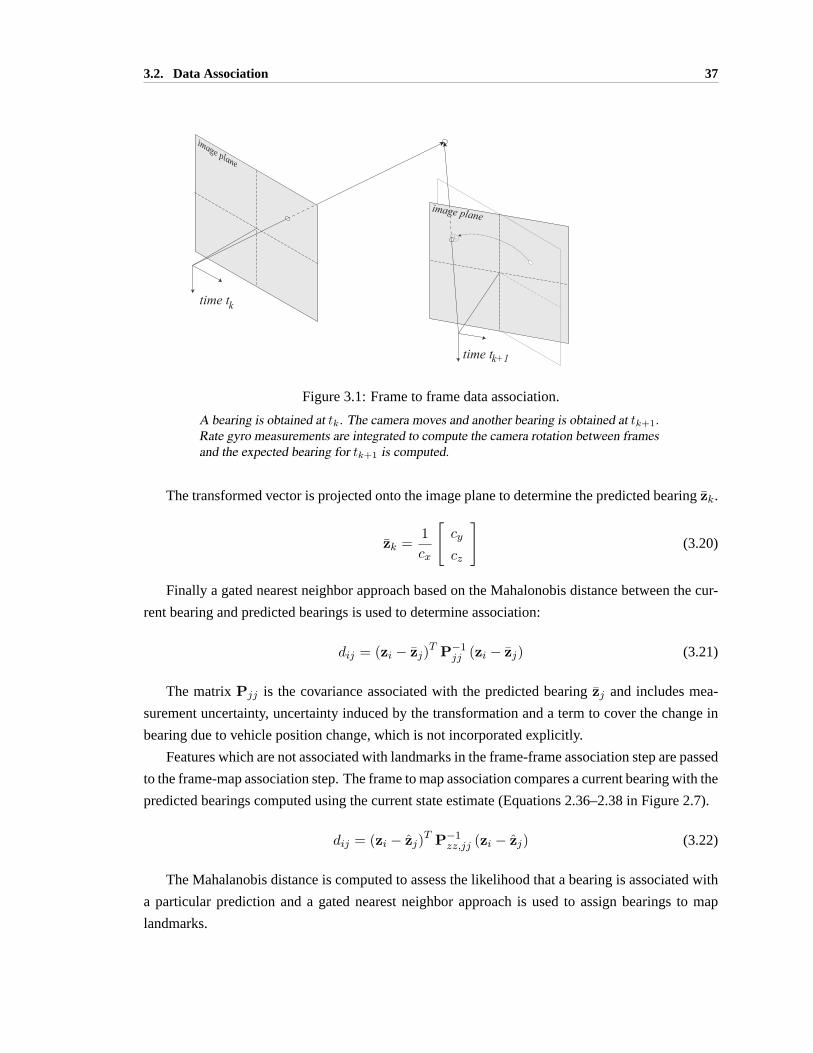
3.2. Data Association 37
image plane
image plane
time tk
time tk+1
Figure 3.1: Frame to frame data association.
A bearing is obtained at tk. The camera moves and another bearing is obtained at tk+1.Rate gyro measurements are integrated to compute the camera rotation between framesand the expected bearing for tk+1 is computed.
The transformed vector is projected onto the image plane to determine the predicted bearingzk.
zk =1cx
[cy
cz
](3.20)
Finally a gated nearest neighbor approach based on the Mahalonobis distance between the cur-
rent bearing and predicted bearings is used to determine association:
dij = (zi − zj)T P−1
jj (zi − zj) (3.21)
The matrixPjj is the covariance associated with the predicted bearingzj and includes mea-
surement uncertainty, uncertainty induced by the transformation and a term to cover the change in
bearing due to vehicle position change, which is not incorporated explicitly.
Features which are not associated with landmarks in the frame-frame association step are passed
to the frame-map association step. The frame to map association compares a current bearing with the
predicted bearings computed using the current state estimate (Equations 2.36–2.38 in Figure 2.7).
dij = (zi − zj)T P−1
zz,jj (zi − zj) (3.22)
The Mahalanobis distance is computed to assess the likelihood that a bearing is associated with
a particular prediction and a gated nearest neighbor approach is used to assign bearings to map
landmarks.
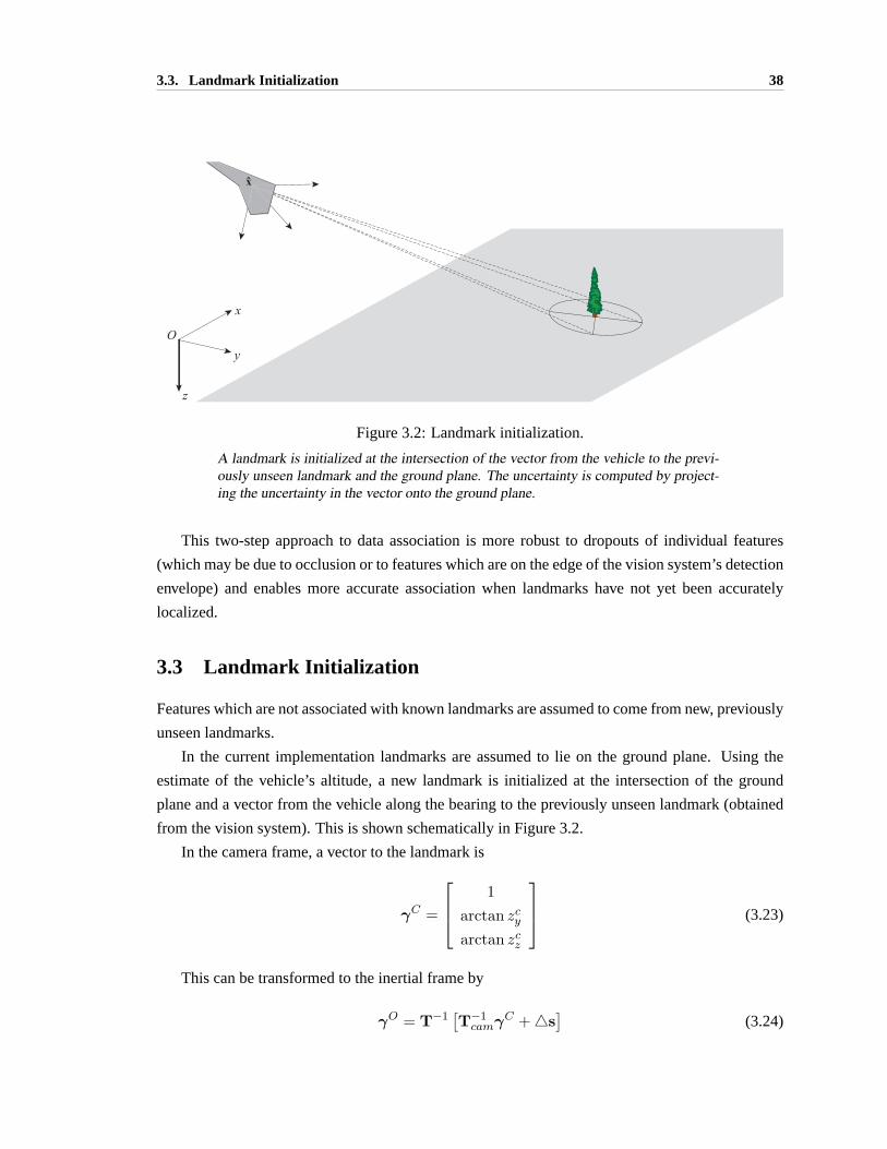
3.3. Landmark Initialization 38
Figure 3.2: Landmark initialization.
A landmark is initialized at the intersection of the vector from the vehicle to the previ-ously unseen landmark and the ground plane. The uncertainty is computed by project-ing the uncertainty in the vector onto the ground plane.
This two-step approach to data association is more robust to dropouts of individual features
(which may be due to occlusion or to features which are on the edge of the vision system’s detection
envelope) and enables more accurate association when landmarks have not yet been accurately
localized.
3.3 Landmark Initialization
Features which are not associated with known landmarks are assumed to come from new, previously
unseen landmarks.
In the current implementation landmarks are assumed to lie on the ground plane. Using the
estimate of the vehicle’s altitude, a new landmark is initialized at the intersection of the ground
plane and a vector from the vehicle along the bearing to the previously unseen landmark (obtained
from the vision system). This is shown schematically in Figure 3.2.
In the camera frame, a vector to the landmark is
γC =
1arctan zcyarctan zcz
(3.23)
This can be transformed to the inertial frame by
γO = T−1[T−1camγC +4s
](3.24)

3.3. Landmark Initialization 39
whereTcam is known andT is computed from the estimates of Euler angles. Uncertainty is present
in both the bearing measurement[zy zz]T and the vehicle orientation (described byT). The vector
γO points from the vehicle to the landmark. The landmark position can now be computed from the
intersection of this vector with the ground plane, since
γO = γ
xi − x
yi − y
zi − z
(3.25)
where[x y z]T denotes the vehicle position in the inertial frame,[xi yi zi]T denotes the landmark
position in the inertial frame andγ is a scale factor. All landmarks are assumed to lie on the ground
plane, hencezi ∼ N (zg,Σg). Therefore:
γ =γOz
zg − z(3.26)
xi =γOxγ
+ x (3.27)
yi =γOyγ
+ y (3.28)
The uncertain parameters leading to the three equations above are: vehicle positionx, y, z;
ground plane heightzg; vehicle orientationφ, θ, ψ (through the transformation in Equation 3.24);
and bearingszCy , zCz .
A sigma-point transform can be used to project the bearing and its associated uncertainty onto
the ground plane. First a state vector is assembled from the current estimate of vehicle position and
orientation, the ground plane height and the bearing measurements:
ξ =[x y z φ θ ψ zg zCy zCz
]T(3.29)
Similarly a covariance matrix is assembled:
Pξ =
Pvv 0 00 Σg 00 0 R
(3.30)
wherePvv is the 6 × 6 covariance associated with the current estimate of vehicle position and
orientation,Σg is the variance of the uncertainty associated with the ground plane height andR is
the covariance of the uncertainty associated with the bearing measurement.

3.4. Estimate Smoothing 40
Using this state vector and associated covariance, a set of Sigma Points is computed using
Equation 2.32. The Sigma Points are propagated through Equations 3.23–3.28 and finally the esti-
mated landmark positionxnew and associated covariancePnew are computed using Equations 2.34
and 2.35. The system state vector is then augmented with the new landmark:
xk|k =
[xk|kxnew
]Pk|k =
[Pk|k 0
0 Pnew
](3.31)
While the augmented state covariance is initially block diagonal, the uncertainty in the new
landmark position quickly becomes correlated with both the vehicle state uncertainty and the uncer-
tainty in previously observed landmark positions.
This method of landmark initialization can be extended to non-planar ground if the vehicle has a
digital elevation map (DEM) of the surrounding terrain. A landmark would now get initialized at the
intersection of the bearing vector and the ground as given by theDEM. There is one caveat however:
as the grazing angle between the ground and the bearing becomes small the projected uncertainty
will become very large. Additionally, the projected uncertainty will no longer be Gaussian, leading
to potential problems when the landmark is added to the estimator.
3.4 Estimate Smoothing
Bearing measurements provide no information about vehicle absolute position or about landmark
absolute position. Absolute position is therefore unobservable, and unless additional information
in the form of absolute measurements are available the estimates of vehicle and landmark absolute
position will drift.
In most SLAM implementations (including this one) the uncertainty in all the states becomes
highly correlated over the course of vehicle motion. Hence additional information about any of
the states can be used to improve the estimates of all the states. This information may come from
many sources: loop closure, which consists of revisiting previously explored terrain; observation of
a priori known landmarks; or sporadicGPSupdates2. With this additional information a smoothing
algorithm can correct the drift in absolute vehicle and landmark positions.
Smoothing of the full vehicle trajectory provides the most accurate correction of the map. How-
ever, this requires enough data that the vehicle trajectory can be reconstructed: this may consist of
all measurements (both inertial and bearings) obtained through the trajectory or it may consist of
retaining vehicle state estimates and the associated covariance throughout the trajectory (i.e. rather
than only including the current vehicle state estimate in the state vector, the current state and all
previous states are included). The state vector will then grow with time, as current vehicle states are
2Arguably observation of a priori known landmarks andGPSupdates are equivalent: both are measurements to whatare effectively beacons.

3.5. Data Flow 41
augment state vectorprediction
measurement dataassociation
landmarkinitialization
visionupdate
xk|k-1^
Pk|k-1
xk|k^
Pk|k
zk zknew
zkold xnew
^
Pnew
correction/smoothing
iaddIadd
Figure 3.3: Flow of estimation.
The estimation process is initialized at the junction labeled ?.
added, as well as with distance, as new landmarks are observed. Both techniques greatly increase
both the storage and computational requirements of the smoothing step.
Rather than smoothing the full vehicle trajectory, a correction step can be applied using only
the current estimate of vehicle state and obstacle positions. This results in a less effective map
correction but does not require storage of all measurements or of all previous vehicle states.
Estimation happens in the state space (i.e.x, P). The correction happens in information space:
I = P−1 i = Ix (3.32)
wherex is the current estimate of the system state andP is the estimated covariance. The correction
step is
Icorr = I + Inew (3.33)
icorr = i + inew (3.34)
whereInew is the information matrix andinew is the information vector associated with the addi-
tional state knowledge. The corrected state and covariance are then recovered:
Pcorr = I−1corr xcorr = Pcorricorr (3.35)
3.5 Data Flow
The flow of data through the estimation process is shown schematically in Figure 3.3.
The estimator is initialized at timet0 with
x0|− = x0 (3.36)

3.5. Data Flow 42
P0|− = P0 (3.37)
If there are any landmarks known a priori, they are included inx0 andP0, otherwise only
vehicle states are present in the initial state vector.
At some timetk:
• Prediction
Predictions of system statexk|k−1 and covariancePk|k−1 are computed using the previous
estimates of state and covariance, system kinematics (Equation 3.16) and theUKF prediction
step equations (Equations 2.32–2.35).
• Measurement
Bearings are obtained from the vision system.
• Data Association
If there are any landmarks in the state vector, data association is performed, following the
two-step process described in Section 3.3. Predicted measurements are computed using the
vision model (3.18), predicted system state and covariance andUKF correction step equations
(Equations 2.36–2.38). Bearings associated with known landmarks (i.e. those already in the
state vector) are placed in an arrayzold, unassociated bearings are placed in an arrayznew
• Vision Update
Bearingszold associated with known landmarks are used to correct the prediction of sys-
tem state usingUKF correction step equations (Equations 2.39–2.42), producingxk|k and the
associated covariancePk|k
• Landmark Initialization
Using the recently corrected system state and covariance and the unassociated bearingsznew,
initial landmark positionsxnew and covariancePnew are computed using the landmark ini-
tialization process described in Section 3.4.
• State Augmentation
The state vector is augmented with the new landmarks so that
xk|k =
[xk|kxnew
]Pk|k =
[Pk|k 0
0 Pnew
](3.38)
• Correction/Smoothing
If additional information is available, correct the current state estimate using Equations 3.33–
3.35.

3.5. Data Flow 43
• Return to Prediction
The process continues recursively.

Chapter 4
UAV Simulation Results
THIS CHAPTER DESCRIBESresults of computer simulations ofUAV flight in unknown, cluttered
environments. The simulations serve two main purposes: first, to demonstrate that standard
estimation techniques (i.e. theEKF) often fail to provide a convergent solution to the problem of
estimating vehicle and landmark states; second, to examine the performance of the estimator, the
data association algorithm and the landmark initialization algorithm presented in Chapter 3. Results
of hardware tests and simulations for a small autonomous rover are described in Chapter 5.
Simulation results are presented to address: (a) estimate consistency; (b) fusion of state esti-
mates with a trajectory planner; (c) vehicle position estimate error growth characteristics.
Results of Monte Carlo simulations of flight in a planar environment show thatconsistentes-
timates of system state (i.e. vehicle position, orientation and velocity,IMU biases, and obstacle
positions) are computed by theUKF-based estimator presented in Chapter 3. A consistent estima-
tor is unbiased (i.e. the mean estimate error is zero) and accurately computes the covariance of
the estimate error. Conversely, a baselineEKF-based approach fails to provide reliably convergent
estimates of vehicle state and obstacle positions.
Next, results of a simulation demonstrating obstacle avoidance in a cluttered planar environment
are presented. This requires an obstacle avoidance algorithm. In this case a randomized motion
planner used the estimates of state and covariance (i.e. the uncertainty in the estimate) to generate
trajectories that minimized the probability of collision while navigating to a goal.
Simulations ofUAV flight in three dimensions address the question of error growth of the vehicle
position estimate. Two flight conditions are considered: exploration, where new landmarks are
continually encountered; and station keeping, where the vehicle orbits a fixed point, either keeping
a set of landmarks in continuous view or cyclically revisiting landmarks. For exploration flight
error was a percentage of distance traveled, for station keeping flight error varied cyclically with
each orbit.
44

4.1. Navigation in a Plane 45
When data association is known a priori the error varied inversely with the square root of the
number of landmarks in view. The data association and landmark initialization algorithms presented
in Sections 3.2 and 3.3, respectively, were tested by examining their effect on the vehicle position es-
timate error. Results showed that data association was successful as long as less than approximately
five landmarks were in view.
An error in data association has the potential to cause divergence of the state estimate, and
increasing the number of landmarks in view increases the likelihood of errors in data association.
Moreover, estimated vehicle states are used to aid both data association and landmark initialization,
hence significant coupling can be expected. Intuition therefore suggests, and simulations showed,
that there is some value of number of landmarks in view which minimizes the estimate error. For the
simulations conducted here, an average of 2.6 landmarks in view minimized the position estimate
error for exploration flight and an average of 5 landmarks in view minimized the position error for
station keeping flight.
Section 4.1 discusses estimate consistency and demonstrates a simulation of flight through a
cluttered environment using 2D simulations. Section 4.2 discusses results of 3D simulations inves-
tigating vehicle position error and Section 4.3 summarizes results.
4.1 Navigation in a Plane
In this section data association and landmark initialization are assumed to be known a priori. This
isolates the estimation problem, allowing a focus on consistency and comparison with anEKF-based
implementation. This section shows:
1. Standard estimation techniques (i.e. the Extended Kalman Filter) fails even for the 2D case
of this estimation problem.
2. The application of an Unscented Kalman Filter results in a consistent, unbiased estimator.
3. Navigation through a cluttered environment is enabled by using results of the estimator cou-
pled with a trajectory planner.
For ease of visualization, simulations were conducted for navigation in a plane. The state vector
x = [xTv xT1 · · · xTm]T contains vehicle states and obstacle positions. For the 2D case the vehicle
state vector is
xv =[x y ψ u v αx αy bx by bψ
]T(4.1)
wherex, y, ψ denote vehicle position and orientation in the inertial frame;u and v denote
velocity expressed in the body frame;αx andαy denote accelerometer scale factor errors in the
bodyx andy directions; and finallybx, by andbψ denote bias errors for the accelerometerx andy

4.1. Navigation in a Plane 46
directions and the rate gyro. The obstacle position
xi =[xi yi
]T(4.2)
includes the obstacle location in the inertial frame.
4.1.1 Estimate Consistency
Kalman filters propagate an estimate of system state and an estimate of the covariance of the estimate
error. Aconsistentestimator is both unbiased (i.e. the expected value of the estimate error is zero)
and accurately estimates the covariance of the estimate error:
E(xk − xk) = 0 (4.3)
E((xk − xk)(xk − xk)T ) = Pkk (4.4)
Alternatively,
E((xk − xk)T (xk − xk)) = Tr(Pkk) (4.5)
Hence to evaluate consistency of the navigation solution one can compare the 2-norm of the
estimate error with the square root of the trace of the covariance matrix. This can be done using
Monte Carlo simulations.
4.1.2 System Equations for the Planar Case
As with the 3D case the time update step is represented by vehicle kinematics, driven by inertial
measurements.
x = cosψu− sinψv (4.6)
y = sinψu+ cosψv (4.7)
ψ = zr − br (4.8)
u =zxαx
− bx + (zr − br)v − bx(ρ) (4.9)
v =zyαy
− by − (zr − br)u− by(ρ) (4.10)
Here[zx zy zψ]T represent the measured acceleration and angular rate.b(·)(ρ) is the acceleration
induced by the (assumed known) offset of theIMU from the vehicleCG and angular rate and angular
acceleration.

4.1. Navigation in a Plane 47
−20 −10 0 10 20
−20
−10
0
10
20
x
yFigure 4.1: Nominal data for 2D Monte Carlo simulations.
Schematic of a single run of the Monte Carlo simulation. Aircraft speed is 10m/s, turnrate is 0.5rad/s, resulting in a turn radius of 20m. The aircraft travels a distance of200m, approximately 1.6 times around the circular path.
The 2D vision measurement model is
zi = arctansi,ysi,x
+ nc (4.11)
wherenc is zero mean Gaussian noise andsi,x andsi,y are the components of the vector from
the vehicle to the landmark expressed in the camera frame:
si = Tcam
[T
[xi − x
yi − y
]−4s
](4.12)
The offset between the camera and the vehicleCG is4s. The rotation matrixTcam transforms
a vector from the body frame to the camera frame, the rotation matrixT transforms a vector from
the inertial frame to the body frame:
T =
[cosψ sinψ− sinψ cosψ
](4.13)
As with the full 3D system equations, the 2D case of state estimation is highly nonlinear.
4.1.3 Monte Carlo Simulation Results
The UAV is flown in a circular trajectory of radius 20m at a velocity of 10m/s through a forest of
randomly distributed trees (see Figure 4.1). A new forest was generated for each run.UAV position
and velocity was assumed to be known accurately at the start of each run (σ2 = 1 × 10⁻⁶) and
landmark positions were assumed to be known with a standard deviation of 1m (i.e. an initial, but

4.1. Navigation in a Plane 48
Table 4.1: IMU initialization parameters for 2D simulations.
αx αy bx by bψ
mean 1 1 0.15 0.10 0.004σ 0.01 0.01 0.1 0.1 0.02
uncertain, map was provided for each run). Estimates ofIMU biases were initialized with a Gaussian
random number using parameters given in Table 4.1.
Since the purpose of the estimator is to determine vehicle state and obstacle positions with an
accurate assessment of the estimate error, success of a run is determined by comparing the estimated
standard deviation of the error with the true standard deviation of the error. These are:
σk,est =√TrPkk (4.14)
σk,truth =√
(xk − xk)T (xk − xk) (4.15)
Where for a consistent estimatorEσk,est = Eσk,truth (Equation 4.5).
Results of a 1000 run Monte Carlo simulation are shown graphically in Figure 4.2. Each plot
shows the envelope of the true variance of estimate error (i.e. the minimum and maximum values
of the 2-norm of the estimate error over all runs at each time step) as a grey region, the mean of the
true variance of estimate error at each time step as a blue line and the mean of the estimated error
variance (i.e.√TrPkk) at each time step as a dashed red line. TheEKF implementation (upper
plot) shows clear divergence of the estimate, with true variance an order of magnitude greater than
the estimated variance. Conversely theUKF implementation (lower plot) shows a well-behaved
estimator with the expectations of true and estimated variance aligned and a narrow envelope of
true variance.
A run is ultimately deemed successful if the estimate error at the end of the run is less than the
estimate error at the state of the run (i.e. information has been gained about the vehicle and the
environment):
σK,truth < σ1,truth (4.16)
Figure 4.3 shows a cumulative distribution plot of the error ratioσK,truth
σ1,truthfor the UKF-based
implementation (solid blue line) and theEKF-based implementation (dashed red line) for 1000 runs.
All of the UKF-based estimators resulted in improved knowledge of the environment, only 205
EKF-based estimators resulted in improved knowledge of the environment.
The estimated state covariance is an assessment of the uncertainty in the estimates of the state
variables. It can be used in trajectory planning to generate paths which minimize the probability of
collisions with obstacles, hence accurate estimation of the estimate error covariance is an important
characteristic of a successful estimator.

4.1. Navigation in a Plane 49
time (s)
estim
ate
erro
r σ
EKF implementation
0 5 10 15 201
10
100
1000
truth envelopetruthestimated
time (s)
estim
ate
erro
r σ
UKF implementation
0 5 10 15 200
2
4
6
8
10
truth envelopetruthestimated
Figure 4.2: Estimator consistency for 2D navigation.
A comparison of estimated standard deviation of the estimate error and true standarddeviation of the estimate error for the EKF implementation (above) and UKF implemen-tation (below). Note the difference in scales. Results are from a 1000 run Monte Carlosimulation. The mean of the true standard deviation of estimate error is shown in blue,mean of estimated standard deviation of estimate error is shown in red. The shaded arearepresents the envelope of the true error variance over 1000 runs.

4.1. Navigation in a Plane 50
0.1 1 10 1000
200
400
600
800
1000
start/end error ratio
num
ber
EKF error ratioUKF error ratio
Figure 4.3: Change in estimate error over course of run.
A cumulative distribution plot of the number of runs which resulted in a reduction inestimate error over the course of each run. All UKF runs resulted in a reduction in trueerror (i.e. error ratio< 1), only 205 EKF runs resulted in reduced true error.
Table 4.2: Maximum and minimum standard deviation ratios
Only results for successful runs (as defined in Equation 4.16) are presented.
max (1 + δ) min (1 + δ) mean(1 + δ)
UKF(1000 runs) 1.73 0.56 1.05EKF(205 runs) 2.62 0.75 1.46
The standard deviation of the estimate error at the end of a run can be used as an assessment of
the best-case and worst-case performance. If a run is successful (i.e.σK,truth < σ1,truth)
σK,truthσK,est
= 1 + δ where δ > −1 (4.17)
For a “good” estimatorδ ≈ 0, indicating that the estimated state uncertainty accurately repre-
sents the true state uncertainty.δ > 0 indicates that the estimated state uncertainty underpredicts
the true state uncertainty, increasing the likelihood of collisions with obstacles.δ < 0 indicates that
the estimated state uncertainty is overpredicted, leading to inefficient trajectories. Note that if the
estimate did not converge thenδ would continue to grow without bound, and thus would not be a
meaningful assessment of performance. In any case, a diverged estimate indicates failure.
Maximum, minimum, and mean values of(1 + δ) are given in Table 4.2 for successful runs.
Figure 4.2 showed that all runs for theUKF-based estimator converged. The largest value of(1 + δ)for the UKF was 1.73, indicating that the end-of-run true standard deviation of the estimate error
does not exceed the end-of-run estimated standard deviation of the estimate error by more than

4.2. 3D Simulations 51
73%. The mean value of(1 + δ) is 1.05, indicating that on average the true error was accurately
predicted by the estimated covariance. Conversely, theEKF-based implementation was unsuccessful
for 795 runs, indicated by the increase in estimate error. For the remaining 205 successful runs, the
worst-case value of(1+δ) was 2.62, indicating that the true error is 162% greater than the estimated
error. On average (for successful runs only) the true error exceeded the estimated error by 46%.
4.1.4 Navigation and Obstacle Avoidance
Section 4.1.3 showed that aUKF-based estimator provides a convergent, consistent estimate of ve-
hicle position, orientation and speed and of obstacle positions. Flight in an obstacle-strewn environ-
ment also requires an algorithm for obstacle avoidance and navigation. In this section a Randomized
Motion Planner [17] is used: a sequence of random inputs is generated and the cost of each trajec-
tory is computed based on the probability of collision with obstacles (computed from the estimated
obstacle positions and the associated covariance) and final distance from the goal.
To illustrate flight in a cluttered environment Figure 4.4 shows a sequence of images of aUAV
navigating through a forest to a goal. True obstacle positions are shown as blue dots, true vehicle
position is shown as blue ‘wings’. Estimated obstacle positions are shown as red+ with associ-
ated3σ error ellipsoid, estimated vehicle position shown as red ‘wings’ with associated3σ error
ellipsoid. The dotted red line shows the planned trajectory, the blue line shows the actual trajectory
flown. The planned trajectory only accounts for obstacles that have been “seen” by the camera:
unobserved obstacles remain unknown until they enter the field of view.
Early in the flight (upper left image) estimated obstacle positions are highly uncertain, as shown
by the large3σ uncertainty ellipsoids. As the aircraft approaches an obstacle it is localized with
greater accuracy, reflecting both the fact that more measurements to that obstacle have been obtained
and that the measurement geometry permits more accurate localization at shorter range (the ‘spread’
of the uncertainty in the bearing is smaller at close range). The increase in positioning certainty has
the consequence of increased safety during operations close to an obstacle: with greater certainty
in obstacle position come greater certainty of that a planned collision-free path is actually collision-
free.
4.2 3D Simulations
Results of 2D simulations showed that consistent estimates of vehicle position and landmark posi-
tions can be obtained. The focus of this section is on the error growth characteristics of the vehicle
position estimate.
Recall from Section 3.4 that bearings only provide information aboutrelativeposition: absolute
position measurements are not available. The estimator therefore is effectively computing vehicle
odometry using vision and inertial measurements, and growth in estimate error is to be expected.

4.2. 3D Simulations 52
Figure 4.4: Obstacle avoidance and navigation in 2D environment.
The sequence of images shows flight through a 2 D forest to a goal position. Trueobstacle positions are shown as blue dots, true vehicle position is shown as blue ‘wings’.Estimated obstacle positions are shown as red + with associated 3σ error ellipsoid,estimated vehicle position shown as red ‘wings’ with associated 3σ error ellipsoid. Thedotted red line shows the planned trajectory, the blue line shows the trajectory flown.

4.2. 3D Simulations 53
(a) exploration (b) station keeping
Figure 4.5: Exploration versus station keeping
Exploration (left image) is characterized by flight through unexplored terrain, with newlandmarks continually entering and leaving the field of view. Station keeping (rightimage) is characterized by orbits about a fixed point. Landmarks may cyclically enterand leave the field of view, or, if the camera is pointed inwards, may be in continuousview.
The error in vehicle position estimate can be characterized in several ways, and the choice of
characterization is dependent the type of motion undergone by the vehicle (Figure 4.5). In ex-
ploratory motion the vehicle traverses through unexplored terrain, with new landmarks entering the
field of view as old landmarks leave the field of view. In effect the vehicle navigates using visual
odometry, and error is best characterized as a percentage of distance traveled. A second type of
flight that may occur is station keeping, where the vehicle follows a roughly circular path orbiting a
fixed point. Over several orbits the same landmarks will be seen repeatedly, enabling cyclic reduc-
tions in the vehicle position error. Alternatively, if the camera is pointed towards the center of the
orbit the same landmarks may remain in view continuously, further reducing position error. In this
mode error is best characterized as an absolute error relative to true vehicle position. Note, however,
that even when the same features are in constant view the lack of absolute position measurements
will lead to cyclically varying errors in absolute vehicle position estimate.
Error growth is affected by many factors: the number of features in view at any given time,
the length of time a particular feature remains in view and the video frame rate are all critical
parameters. These in turn are affected by feature density, vehicle speed and altitude and camera
field of view.
The focus of this section is on error growth characteristics of the vehicle position estimate in
both exploratory and station keeping flight. This section examines:

4.2. 3D Simulations 54
1. The effect of number of landmarks in view on vehicle position estimate error. Here data
association and landmark initialization are assumed to be solved.
2. The effect of the both the data association algorithm and the landmark initialization algorithm
presented in Sections 3.3 and 3.4, respectively, on the vehicle position estimate.
4.2.1 Estimator Performance
A series of Monte Carlo simulations was conducted for both exploratory and station keeping flight
to examine the effect of the number of landmarks in view on the vehicle position estimate. Both
data association and landmark initialization were assumed to be known.
Results are presented in Sections 4.2.1 and 4.2.2. A discussion of results is given in Section
4.2.3. Noise and initialization parameters for these simulations are given in Appendix B.
Exploration
The vehicle followed a circular trajectory of radius 40m at an altitude of 5m and a speed of 10m/s
for a distance of 200m. Monte Carlo simulations were conducted with varying landmark densities
to vary the number of landmarks in view. For each simulation 500 runs were conducted, with a new
forest generated for each run. In all cases a minimum tree spacing (dependent on the number of
trees) was imposed to minimize “clumping” of landmarks in each forest.
The error in estimated vehicle position is shown in Figure 4.6 for each Monte Carlo simulation.
The mean of the position error is shown as a solid line, the median position error is shown as a
dashed line, and dotted lines show the 5% and 95% position estimate errors.
All runs showed converged estimates. The mean and median errors are roughly equal and lie
midway between the 5% and 95% bounds. As expected, increasing the number of features in view
from an average of 1.35 to 7.87 decreases the median estimate error from 0.67% to 0.36% of the
distance traveled.
Station keeping
The vehicle followed a circular trajectory of radius 200m at an altitude of 100m and a speed of
20m/s for 240 seconds (performing almost 4 orbits). The camera was pointing towards the center of
the orbit, insuring that all features were in continuous view. Seven Monte Carlo simulations were
conducted with 1, 2, 3, 5, 7, 9 and 11 landmarks.
As with the exploration case, each Monte Carlo simulation consisted of 500 runs with a new
forest generated for each run. Again minimum landmark separations (based on the number of
landmarks) were imposed to minimize clumping.
With only one landmark in view the error in vehicle position estimate grew without bound: a
single bearing does not provide enough information to localize the vehicle. The error in estimated

4.2. 3D Simulations 55
0 20 40 60 80 100 120 140 160 180 2000
1
2
3
4
5
6
distance travelled (m)
erro
r (%
dis
tanc
e tr
avel
led)
(a) nview = 1.35
0 20 40 60 80 100 120 140 160 180 2000
1
2
3
4
5
6
distance travelled (m)
erro
r (%
dis
tanc
e tr
avel
led)
(b) nview = 2.64
0 20 40 60 80 100 120 140 160 180 2000
1
2
3
4
5
6
distance travelled (m)
erro
r (%
dis
tanc
e tr
avel
led)
(c) nview = 3.93
0 20 40 60 80 100 120 140 160 180 2000
1
2
3
4
5
6
distance travelled (m)
erro
r (%
dis
tanc
e tr
avel
led)
(d) nview = 5.24
0 20 40 60 80 100 120 140 160 180 2000
1
2
3
4
5
6
distance travelled (m)
erro
r (%
dis
tanc
e tr
avel
led)
(e) nview = 6.53
0 20 40 60 80 100 120 140 160 180 2000
1
2
3
4
5
6
distance travelled (m)
erro
r (%
dis
tanc
e tr
avel
led)
(f) nview = 7.87
Figure 4.6: Exploration vehicle position estimate error, known data association and landmark ini-tialization.
Mean error shown as solid line, median error shown as dashed line, 5% and 95% boundsshown as dotted lines.

4.2. 3D Simulations 56
vehicle position is shown in Figure 4.7 for simulations with 2 or more landmarks in view. The mean
of the position error is shown as a solid line, the median position error is shown as a dashed line,
and dotted lines show the 5% and 95% position estimate errors.
All runs showed converged estimates. The mean and median errors are roughly equal and lie
midway between the 5% and 95% bounds. As expected, increasing the number of features in view
from 2 to 11 decreases the median estimate error from 1.28m to 0.6m. As expected the estimate
error varies cyclically with each orbit.
4.2.2 Effect of Explicit Data Association and Landmark Initialization
A series of Monte Carlo simulations was conducted to assess the effect of explicit data association
and landmark initialization on the performance of the estimator. The algorithms of Sections 3.2
and 3.3 were used to compute data association and landmark initialization, respectively.
An error in data association has the potential to lead to estimator divergence. Increasing the
number of landmarks in view increases the likelihood of errors in data association. It is therefore
expected that divergent estimates will occur as the number of landmarks in view is increased. This
will be manifested as an increase in the number and magnitude of outliers in the estimated position
error, causing a difference in the median and mean estimate error and potentially causing the 95%
bound to increase.
Exploration
As with Section 4.2.1, the vehicle followed a circular trajectory of radius 40m at an altitude of 5m
and a speed of 10m/s for a distance of 200m. Monte Carlo simulations were conducted with varying
landmark densities to vary the number of landmarks in view. For each simulation 500 runs were
conducted, with a new forest generated for each run. In all cases a minimum tree spacing (dependent
on the number of trees) was imposed to minimize “clumping” of landmarks in each forest.
The error in estimated vehicle position is shown in Figure 4.8 for each Monte Carlo simulation.
The mean of the position error is shown as a solid line, the median position error is shown as a
dashed line, and dotted lines show the 5% and 95% position estimate errors.
For small numbers of landmarks in view similar behavior to the known data association and
landmark initialization cases were observed, indicating that data association was generally success-
ful. As the average number of landmarks in view increased, however, clear divergence of some runs
in each Monte Carlo simulation was observed (indicated by the steadily increasing 95% bound for
the cases withnview = 6.56 andnview = 7.87).

4.2. 3D Simulations 57
0 40 80 120 160 200 2400
1
2
3
4
5
6
time (s)
abso
lute
err
or (
m)
(a) nview = 2
0 40 80 120 160 200 2400
1
2
3
4
5
6
time (s)
abso
lute
err
or (
m)
(b) nview = 3
0 40 80 120 160 200 2400
1
2
3
4
5
6
time (s)
abso
lute
err
or (
m)
(c) nview = 5
0 40 80 120 160 200 2400
1
2
3
4
5
6
time (s)
abso
lute
err
or (
m)
(d) nview = 7
0 40 80 120 160 200 2400
1
2
3
4
5
6
time (s)
abso
lute
err
or (
m)
(e) nview = 9
0 40 80 120 160 200 2400
1
2
3
4
5
6
time (s)
abso
lute
err
or (
m)
(f) nview = 11
Figure 4.7: Station keeping vehicle position estimate error, known data association and landmarkinitialization.
Mean error shown as solid line, median error shown as dashed line, 5% and 95% boundsshown as dotted lines.

4.2. 3D Simulations 58
0 20 40 60 80 100 120 140 160 180 2000
1
2
3
4
5
6
distance travelled (m)
erro
r (%
dis
tanc
e tr
avel
led)
(a) nview = 1.37
0 20 40 60 80 100 120 140 160 180 2000
1
2
3
4
5
6
distance travelled (m)
erro
r (%
dis
tanc
e tr
avel
led)
(b) nview = 2.63
0 20 40 60 80 100 120 140 160 180 2000
1
2
3
4
5
6
distance travelled (m)
erro
r (%
dis
tanc
e tr
avel
led)
(c) nview = 3.94
0 20 40 60 80 100 120 140 160 180 2000
1
2
3
4
5
6
distance travelled (m)
erro
r (%
dis
tanc
e tr
avel
led)
(d) nview = 5.24
0 20 40 60 80 100 120 140 160 180 2000
1
2
3
4
5
6
distance travelled (m)
erro
r (%
dis
tanc
e tr
avel
led)
(e) nview = 6.56
0 20 40 60 80 100 120 140 160 180 2000
1
2
3
4
5
6
distance travelled (m)
erro
r (%
dis
tanc
e tr
avel
led)
(f) nview = 7.87
Figure 4.8: Exploration vehicle position estimate error, explicit data association and landmark ini-tialization.
Mean error shown as solid line, median error shown as dashed line, 5% and 95% boundsshown as dotted lines.

4.2. 3D Simulations 59
Station keeping
As with Section 4.2.1, the vehicle followed a circular trajectory of radius 200m at an altitude of
100m and a speed of 20m/s for 240 seconds (performing almost 4 orbits). The camera was pointing
towards the center of the orbit, insuring that all features were in continuous view. Monte Carlo
simulations were conducted with 1, 2, 3, 5, 7, 9, and 11 landmarks.
As with the exploration case, each Monte Carlo simulation consisted of 500 runs with a new
forest generated for each run. Again minimum landmark separations (based on the number of
landmarks) were computed to minimize clumping.
The error in estimated vehicle position is shown in Figure 4.9 for simulations with 2 or more
landmarks in view. The mean of the position error is shown as a solid line, the median position error
is shown as a dashed line, and dotted lines show the 5% and 95% position estimate errors.
For cases with 5 or fewer landmarks in view similar behavior to the estimator only cases were
observed. Fornview = 7 mean error is increasing, indicating that the magnitude of the outliers (but
not the number, since both the 95% bound and the median error are still small) is increasing. For
nview > 7 several runs in each Monte Carlo simulation are clearly diverging (note the difference
in scale). The median errors, however, are not increasing as significantly, again indicating that the
magnitude, but not the number, of outliers in estimated position error is increasing.
4.2.3 Discussion of 3D Simulation Results
Results of the 3D Monte Carlo simulations are summarized in Figure 4.10. Each plot shows the
mean and median vehicle position estimate errors for exploration (left image) and station keeping
(right image).
The estimator only cases (plotted with+) show monotonically decreasing estimate error as the
number of landmarks in view increases. Each landmark provides an independent bearing measure-
ment: therefore the estimate error should vary approximately with1√nview
. To verify this, a least
squares fit was conducted for the assumed function
e =a√
nview + b+ c (4.18)
wheree is the average of the median error of each Monte Carlo simulation. The computed
values of the parametersa, b, andc as well as the 2-norm of the residual are given in Table 4.3. The
small residual indicates the goodness of the fit: as expected the error in vehicle position estimate
varies with 1√nview
.
As expected, results are quite different if data association is not known a priori. When the
number of landmarks in view is small similar behavior to the cases with known data association was
observed, indicating that the data association algorithm of Section 3.2 was generally successful. For

4.2. 3D Simulations 60
0 40 80 120 160 200 2400
1
2
3
4
5
6
time (s)
abso
lute
err
or (
m)
(a) nview = 2
0 40 80 120 160 200 2400
1
2
3
4
5
6
time (s)
abso
lute
err
or (
m)
(b) nview = 3
0 40 80 120 160 200 2400
1
2
3
4
5
6
time (s)
abso
lute
err
or (
m)
(c) nview = 5
0 40 80 120 160 200 2400
1
2
3
4
5
6
time (s)
abso
lute
err
or (
m)
(d) nview = 7
0 40 80 120 160 200 2400
5
10
15
20
25
30
time (s)
abso
lute
err
or (
m)
(e) nview = 9
0 40 80 120 160 200 2400
10
20
30
40
50
60
time (s)
abso
lute
err
or (
m)
(f) nview = 11
Figure 4.9: Station keeping vehicle position estimate error, explicit data association and landmarkinitialization.
Mean error shown as solid line, median error shown as dashed line, 5% and 95% boundsshown as dotted lines.

4.2. 3D Simulations 61
0 1 2 3 4 5 6 7 8 9 100
0.25
0.5
0.75
1
1.25
1.5
average number of landmarks in view
aver
age
erro
r (%
dis
t. tr
avel
led)
median, estimator onlymean, estimator onlymedianmean
(a) exploration
0 2 4 6 8 10 120
0.5
1
1.5
2
2.5
3
3.5
4
4.5
average number of landmarks in viewav
erag
e er
ror
(m)
median, estimator onlymean, estimator onlymedianmean
(b) stationkeeping
Figure 4.10: Effect of landmark density on vehicle position estimate error.
For exploration error is plotted as percentage of distance traveled, for station keepingabsolute error is plotted.
Table 4.3: Error growth parameters
a b c ‖r‖2
exploration 0.525 -0.0373 0.173 0.013station keeping 1.12 -0.80 0.25 0.015

4.3. Summary 62
larger numbers of landmarks in view errors in data association caused progressively larger errors in
position estimate. For the exploration cases the minimum error occurred when the average number
of landmarks in view was 2.62, for exploration the minimum error occurred withnview = 5.
While these results will vary depending on the values of bearing and inertial measurement noise
and flight trajectory parameters, they give a clear indication of the number of landmarks that should
be actively tracked by the estimator. If data association is not known perfectly, no more than three
landmarks should be tracked for exploration and no more than five landmarks should be actively
tracked for exploration. Even with perfect data association, a point of diminishing returns in vehicle
position estimate error is reached at about 5 landmarks tracked for both exploration and station
keeping.
This raises a question of selecting appropriate landmarks when flying through landmark-rich
environments. Using all available landmarks is both computationally intense and prone to failure.
The problem of selecting an optimal set of landmarks is an interesting one.
Landmarks should be geographically diverse: a landmark on a bearing similar to another will
not provide much additional information. In addition, landmarks should be chosen to ensure that
bearings change significantly over time, since it is the change in bearing that provides the informa-
tion necessary to localize the vehicle and the landmark.
4.3 Summary
This chapter has presented results of simulations ofUAV flight in unexplored environments.
2D Simulation
• Estimate consistency: TheUKF-based estimator developed in Chapter 3 provides consistent
estimates of vehicle state and obstacle positions.
• Obstacle avoidance:Using estimates of system state and the estimated covariance a trajec-
tory planner can compute a safe path through a cluttered environment.
3D Simulation
Two classes of flight were investigated with Monte Carlo simulations: exploration, where new
landmarks continually come into view; and station keeping, where the vehicle orbits a fixed point.
• Vehicle position estimate error: With known data association the vehicle position estimate
varies inversely with the square root of the number of landmarks.
• Data association and landmark initialization: As expected, errors in data association gen-
erally lead to divergent estimates. Correct data association is therefore critical to successful
4.3. Summary 63
state estimation. Increasing the number of landmarks in view increases the likelihood of errors
in data association. Therefore there exists a number of landmarks in view which minimizes
the vehicle position estimate error. For the simulations done here, approximately 3 landmarks
in view minimizes vehicle estimated position error for exploration flight and 5 landmarks in
view minimizes vehicle estimated position error for station keeping flight.
• Landmark selection Even when data association is known perfectly a point of diminishing
returns in vehicle position estimate error is quickly reached as the number of landmarks in
view is increased. This suggests that the number of actively tracked landmarks inSLAM
applications should be limited. The actual number will be implementation dependent, but will
have the additional benefit of reducing the computational overhead associated withSLAM.

Chapter 5
Ground Vehicle Results
THE ESTIMATOR DEVELOPED in Chapter 3 and tested in simulation forUAV applications is
now applied to the problem of navigating a small Unmanned Ground Vehicle (UGV). Since a
kinematic model driven by inertial measurements is used for the prediction step both the algorithms
developed earlier and the necessary hardware can in principle be simply “bolted on” to a vehicle
and used for obstacle avoidance and navigation. Both hardware and simulation tests are discussed.
The hardware tests demonstrate successful state estimation using the algorithms presented ear-
lier on an operational system. Real time execution is demonstrated in addition to the ability of
the algorithms to cope with real sensor measurements and model and calibration errors. Further-
more, the hardware tests provide another example of integration of the estimation algorithm with
an obstacle avoidance and navigation algorithm, enabling real-time navigation through a cluttered
environment.
The tests presented in this chapter were conducted using a smallUGV. Although a ground
vehicle nominally has only three degrees of freedom (x andy position and heading), vehicle state
estimation was performed for the six degrees of freedom inherent to aUAV (x and y position,
altitudez, and Euler anglesφ, θ, ψ). The hardware tests examined three subjects: (a) accuracy
of the estimation of states required for aircraft control (i.e. altitude, roll and pitch); (b) estimation
of relative obstacle position; (c) mapping and absolute vehicle localization. Absolute truth data
was available for obstacle positions, vehicle start position and final vehicle position (obtained using
a tape measure). Since it was a ground vehicle, approximate truth data was available for vehicle
altitude, roll and pitch throughout the run.
Results showed that altitude, roll and pitch were estimated accurately (altitude error was gen-
erally within the estimated3σ bound) and the obstacle relative position estimates were accurate
within estimated error. As expected, drift was observed in the absolute vehicle localization and
landmark mapping. However, the drift was larger than the estimated covariance and was similar in
both magnitude and direction for each of the three runs, indicating systemic bias.
64

5.1. Hardware Implementation 65
Two possible causes for the drift are unmodeled offset in camera orientation and poor initial es-
timates of accelerometer bias (i.e. initial estimate error significantly greater than the assumed error).
Simulations showed that an unmodeled camera pitch offset of1◦ results in absolute position esti-
mate errors similar in magnitude and direction to those observed in hardware tests. A vehicle pitch
of 3◦ during IMU initialization would also give absolute position errors similar to those observed in
hardware tests due to the projection of gravity onto the computed initial accelerometer biases.
When additional state information is available (e.g. because the vehicle travels to a known
goal location) drift in vehicle localization and the map can be corrected (Section 3.4). InSLAM
implementations the uncertainty in vehicle position and landmark positions becomes fully correlated
over the course of vehicle motion. Additional knowledge about one of the states (e.g. vehicle
position) can therefore be used to correct the estimates of all states. Additional knowledge of vehicle
position may be obtained by revisiting previously explored areas (loop closure) or by sporadicGPS
updates. The correction step requires the full covariance matrix, which was not available in the
hardware tests. Simulation results are used to illustrate map correction.
Section 5.1 describes the hardware implementation and Section 5.2 describes the test setup.
Section 5.3 describes results of vehicle state estimation, Section 5.4 describes results of obstacle
relative position estimation and Section 5.5 presents results of vehicle absolute position estimation
and mapping. Results are summarized in Section 5.6.
5.1 Hardware Implementation
The ground vehicle “Squirrel” (Figure 5.1) is based on an electric RC truck platform. It carries an
inertial measurement unit, radio modem, camera and analog video transmitter.
Data from the camera andIMU are transmitted to a ground station via wireless links, where
all computation is performed. Commands are subsequently sent to the vehicle through a modified
RC transmitter. The ground station consists of a 3.0GHz Xeon dual-processor desktop computer, a
Matrox Meteor II frame grabber, a 2.4GHz receiver for analog video, a Maxstream 900MHz radio
modem and a modified 72MHz RC transmitter.
The navigation system can be loosely divided into four subsystems: a vision subsystem, which
provides bearings to landmarks in the environment; an inertial subsystem, which provides acceler-
ations and angular rates; the estimator; and a path planning and control subsystem (see Figure 5.2).
5.1.1 Vision Subsystem
The camera is a Panasonic KX-131 CCD camera equipped with a115◦ field of view lens. Resolution
is 380 lines by 640 pixels per line. This is converted to NTSC before analog transmission over a

5.1. Hardware Implementation 66
Figure 5.1: The autonomous ground vehicleSquirrelused as testbed.
camera2.4GHz Tx
IMU
framegrabber
900MHz Tx
2.4GHz Rx
900MHz Rx
featureextraction
estimator
planner/control 72MHz Tx
72MHz Rx servos
base station mobile
vision subsystem
inertial subsystem
planning/control subsystem
Figure 5.2: Schematic of mapping/navigation system.
Data is collected and transmitted to the ground station using a 2.4GHz analog trans-mitter for the video and 900MHz radio modem for inertial measurements. Controlcommands are sent to the vehicle via a modified 72MHz RC transmitter.

5.1. Hardware Implementation 67
Table 5.1: Typical 1σ measurement noise for IMU portion of Phoenix-AX autopilot module.
acceleration (m/s2) angular rate (rad/s)x y z x y z
0.085 0.080 0.062 0.0084 0.0098 0.0078
2.4GHz wireless link to the groundstation. A Matrox Meteor II framegrabber captures frames at
10Hz.
Each frame is blurred using a 5 pixel×5 pixel Gaussian filter and downsampled to 320×240
pixels. The downsampled image is further blurred with a 5 pixel×5 pixel flat filter prior to segmen-
tation. Color segmentation is done in the HSV color space (Hue, Saturation, Value) to recognize
red blobs, which have been defined as landmarks/obstacles. Blobs smaller than 15 pixels square are
ignored to reduce the effect of noise and spurious feature detection. Blobs which touch the edge of
the frame are also ignored. A standard lens distortion correction algorithm [6] is applied to thexy
pixel location of the centroid of each blob.
The wireless link is subject to dropouts caused by interference, multipath and occlusion, hence
the estimator must be robust to data losses in the vision subsystem.
5.1.2 Inertial Subsystem
The inertial measurement unit is part of the Phoenix-AX Autopilot Module [40] supplied by O-
Navi LLC [39]. In this application accelerations and angular rates (along with a packet checksum)
are transmitted over an RS-232 link using a 900MHz radio modem to a ground station at a rate
of approximately 100Hz. At the ground station this is downsampled to 50Hz by averaging. This
reduces the effect of a lost packet.
Noise levels and starting values for biases are obtained prior to each run by keeping the unit
approximately level and stationary for a period of time. The mean and standard deviation of the
signals provide bias and noise, respectively. Typical noise levels are given in Table 5.1.
5.1.3 Path Planning and Control
Planning and control are not the focus of this dissertation. However, to demonstrate vehicle navi-
gation in a cluttered environment an algorithm for path planning and vehicle control is necessary.
Due to its ease of implementation a potential field approach was used for obstacle avoidance and
navigation to the goal. A cost function dependent on the distance from the goal and distance from
obstacles is computed:
c = (xg − x)TWg(xg − x) +N∑i=1
[(xi − x)TP−1
ii (xi − x) + (xi − x)T (xi − x)]
(5.1)

5.2. Test Description 68
Herexg is the goal location in absolute coordinates,x is the current estimate of absolute vehicle
position andWg is a weighting matrix. Both the Mahalanobis distance and the Euclidean distance
from obstacles is used for collision avoidance.xi is the estimated obstacle position,Pii is the uncer-
tainty in estimated position. The Mahalanobis distance essentially computes the distance between
the vehicle and an obstacle as a number of standard deviations: the inverse of the Mahalanobis dis-
tance is a measure of the likelihood of collision. The Euclidean distance is included to insure that
separation is maintained even when the uncertainty in obstacle estimated position is small.
The vehicle steering angle is computed based on the cross product of the estimated vehicle
velocity (in absolute coordinates) and the gradient of the cost function:
γ = K arcsin(
vg ×∇c|vg||∇c|
)(5.2)
Herevg is the estimated vehicle velocity expressed in the inertial frame andK is a gain.
Potential field algorithms are subject to local minima and generally require tuning of parameters
to be effective. For the hardware tests described in this chapter no significant tuning was performed.
5.2 Test Description
Figure 5.3 shows the artificial “forest” used for testing. A “tree” consisted of a 2.1m tall pole topped
with an red inverted cone. The red cone provided the visual target for landmark identification and
the 2.1m height defined the “ground plane” for feature initialization (see Section 3.4). Thirteen trees
were placed randomly over an area of approximately 25m×6m. A set of three pylons were placed
to define a common coordinate frame and a goal location was defined in relation to the coordinate
frame.
At the start of each run the vehicle was placed at (-3,1) in the coordinate frame defined by the
three pylons. No attempt was made to level the vehicle. Each run began with the vehicle remaining
stationary for 10 seconds while inertial measurements (acceleration and angular rates in three axes)
were collected. The average value of acceleration and angular rate in each axis over 10 seconds
was computed as an initial estimate of bias, the standard deviation was used for measurement noise.
After IMU initialization was completed the vehicle was commanded to drive to the goal location
at approximately (22,1.8). Three runs were conducted to investigate: the quality of state estimates
that are required for control of aUAV (altitude, roll, pitch); obstacle relative position estimation;
absolute vehicle position estimation and mapping.
Because of test limitations truth data was only available for obstacle absolute position (obtained
with a tape measure) and vehicle position at the end of the run (obtained with a tape measure).
Approximate truth was available for vehicle altitude, roll and pitch angle. True vehicle altitude can
be approximated quite well as zero, true vehicle orientation was within a few degrees of zero. While

5.3. Vehicle State Estimation 69
Figure 5.3: The artificial “forest” used for hardware tests.
the vehicle body was nominally flat, a slight roll to the right (positive roll) and pitch up (positive
pitch) was observed while the vehicle was in forward motion. This was due to drive train torque. In
addition, testing was conducted outdoors on a sports field, which was quite bumpy on the scale of
the vehicle. The bumps did not significantly affect altitude but did have a noticeable effect on pitch
and roll.
5.3 Vehicle State Estimation
Figures 5.4–5.6 show the number of landmarks in view, altitude estimate error, estimated roll and
estimated pitch for the three runs. In each of the runs, on average approximately three landmarks
were in view at any time, from a minimum of one to a maximum of six (the brief spike to nine at
37s in run 3 is due to a frame error in the vision system).
The error in estimated altitude (z − z, wherez = 0) remains generally within the estimated3σbounds for each of the runs. The estimated standard deviation of the altitude estimate error is less
than 0.1m for each of the three runs.
Simulation results presented in Chapter 4 showed that the error in position estimate varies in-
versely with the square root of the number of features in view. This dependence of estimated covari-
ance on number of features in view is also seen in hardware tests: comparingσz with the number

5.3. Vehicle State Estimation 70
0
2
4
6
8
10
num
ber
landmarks in view
−0.6
−0.3
0
0.3
0.6
met
ers
altitude error
−6
−3
0
3
6
degr
ees
estimated roll
15 20 25 30 35 40 45 50 55 60 65−6
−3
0
3
6estimated pitch
degr
ees
time (s)
Figure 5.4: Estimated vehicle states, run 1.
The upper plot shows the number of landmarks in view, the second plot shows the errorin altitude estimate (blue) along with 3σ bounds (dashed red). The third and fourthplots show estimated roll and pitch, respectively.
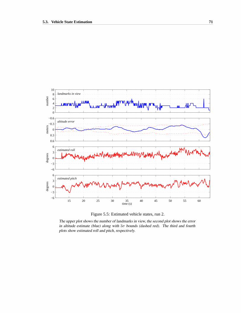
5.3. Vehicle State Estimation 71
0
2
4
6
8
10
num
ber
landmarks in view
−0.6
−0.3
0
0.3
0.6
met
ers
altitude error
−6
−3
0
3
6
degr
ees
estimated roll
15 20 25 30 35 40 45 50 55 60−6
−3
0
3
6estimated pitch
degr
ees
time (s)
Figure 5.5: Estimated vehicle states, run 2.
The upper plot shows the number of landmarks in view, the second plot shows the errorin altitude estimate (blue) along with 3σ bounds (dashed red). The third and fourthplots show estimated roll and pitch, respectively.

5.3. Vehicle State Estimation 72
0
2
4
6
8
10
num
ber
landmarks in view
−0.6
−0.3
0
0.3
0.6
met
ers
altitude error
−6
−3
0
3
6
degr
ees
estimated roll
15 20 25 30 35 40 45 50 55 60 65−6
−3
0
3
6estimated pitch
degr
ees
time (s)
Figure 5.6: Estimated vehicle states, run 3.
The upper plot shows the number of landmarks in view, the second plot shows the errorin altitude estimate (blue) along with 3σ bounds (dashed red). The third and fourthplots show estimated roll and pitch, respectively.

5.4. Obstacle relative position estimation 73
Table 5.2: Results of vehicle state estimation
run nview ‖z − z‖ σz σφ σθm m deg. deg.
1 2.83 0.12 0.063 0.28 0.242 3.03 0.083 0.058 0.29 0.243 2.66 0.15 0.063 0.29 0.24
of landmarks in view (nview) shows that a decrease innview leads to an increase inσz. Conversely
increasingnview leads to a decrease inσz.
The number of landmarks in view is generally very ‘noisy’, jumping rapidly as landmarks on
the edge of the detection envelope enter and leave.
There is a sharp spike in estimated roll as the vehicle starts moving (at approximately 12s in
each run). The vehicle body did in fact roll sharply to the right (positive roll) at the beginning of
motion due to drive train torque. After the initial spike a slight positive roll remained throughout the
run, caused by drive train torque. This can be seen in the estimated roll. The estimated roll angle
is very jagged. This may be partially due to noise in the estimate, but the ground was very bumpy,
leading to significant bumps and jogs in the body orientation throughout each run.
Similar behavior can be seen in the pitch estimate. Again a slight positive pitch was observed in
the vehicle body while it was underway.
Results are tabulated in Table 5.2.
5.4 Obstacle relative position estimation
Relative obstacle position estimation is critical for obstacle avoidance. To illustrate the accuracy of
relative position estimation, Figures 5.7–5.9 show[xi
yi
]−
[xi − x
yi − y
](5.3)
for obstacles in the vicinity of the vehicle. Here[xi yi]T is the true position of theith obstacle,
[xi yi]T is the estimated position of theith obstacle and[x y]T is the estimated vehicle position. In
other words, the plots show the estimated relative vehicle position with respect to the true obstacle
positions. Blue dots show absolute obstacle positions, the open blue circle shows true final vehi-
cle position. The red+ with associated3σ error ellipsoid shows estimated relative position of the
vehicle with respect to an obstacle, where the dotted red line and circle show which obstacle is as-
sociated with a particular relative position estimate. Accurate relative position estimates are shown

5.5. Mapping 74
when the estimates of relative vehicle position with respect to each obstacle agree within estimated
covariance (i.e. when the error ellipsoids overlap).
For each of the three runs the ellipsoids representing3σ uncertainty in the relative position
estimates generally lie on top of one another, indicating that relative position estimation is accurate
within estimated error.
5.5 Mapping
Recall from Chapters 3 and 4 that the lack of absolute position measurements inevitably leads to
drift in the absolute vehicle and landmark position estimates. If there are no unmodeled dynamics or
biases in the system (e.g. an unmodeled offset in camera orientation) the drift can be characterized
as a random walk and will be described by the estimated error covariance. If there are unmodeled
biases they will be reflected by a bias in the vehicle position and obstacle position estimates.
Figures 5.10–5.12 show absolute vehicle position estimates and absolute landmark position es-
timates as a sequence of images over the course of each run. Blue dots show absolute obstacle
positions. The open blue circle shows true final vehicle position. The red+ with associated3σerror ellipsoid shows estimated obstacle position, estimated vehicle position is shown by the red
“wings” and associated3σ error ellipsoid. The estimated vehicle path is shown by the red line.
Early in each run absolute obstacle position estimates are quite good, but a bias builds up in all
obstacle position estimates as the run progresses. This error is also seen in the final vehicle position
estimate, which is offset from the true final vehicle position. The offset is of similar magnitude and
direction in all three runs, indicating that a systemic bias is likely.
Effects of some possible error sources
There are many possible sources of systemic bias. Two are an unmodeled offset in camera orien-
tation and a poor initial estimate of bias. Intuitively, an offset in camera orientation should result
in a biased map because the camera provides information about the surrounding landmarks. Sim-
ilarly, a poor estimate of accelerometer bias will result in an error in the estimate of the baseline
between successive camera images, leading to an error in both landmark relative position estimates
and vehicle position estimates.
To illustrate the effect of these possible error sources simulations of the outdoor tests with
unmodeled errors are presented.
Figure 5.13 shows the effect of an unmodeled1◦ offset in camera pitch. This offset in camera
orientation causes errors in two ways: first, by introducing a bias in the initial landmark position,
and second by introducing a bias in the vehicle position correction.
The map generated with camera pitch offset shows similar behavior as observed in the hardware
tests: initial map accuracy is good, but the vehicle position estimate and mapped landmark positions

5.5. Mapping 75
0 5 10 15 20 25 30
−2.5
0
2.5
5
x (m)
y (
m)
time: 11.2 s
0 5 10 15 20 25 30
−2.5
0
2.5
5
x (m)
y (
m)
time: 30.2 s
0 5 10 15 20 25 30
−2.5
0
2.5
5
x (m)
y (
m)
time: 51.2 s
0 5 10 15 20 25 30
−2.5
0
2.5
5
x (m)
y (
m)
time: 68.8 s
Figure 5.7: Sequence of relative position estimates, run 1
Blue dots show absolute obstacle positions. The open blue circle shows true final ve-hicle position. The red + with associated 3σ error ellipsoid shows estimated relativeposition of the vehicle with respect to an obstacle, where the dotted red line and circleshow which obstacle is associated with a particular relative position estimate.

5.5. Mapping 76
0 5 10 15 20 25 30
−2.5
0
2.5
5
x (m)
y (
m)
time: 11.2 s
0 5 10 15 20 25 30
−2.5
0
2.5
5
x (m)
y (
m)
time: 30.2 s
0 5 10 15 20 25 30
−2.5
0
2.5
5
x (m)
y (
m)
time: 40.2 s
0 5 10 15 20 25 30
−2.5
0
2.5
5
x (m)
y (
m)
time: 63.8 s
Figure 5.8: Sequence of relative position estimates, run 2
Blue dots show absolute obstacle positions. The open blue circle shows true final ve-hicle position. The red + with associated 3σ error ellipsoid shows estimated relativeposition of the vehicle with respect to an obstacle, where the dotted red line and circleshow which obstacle is associated with a particular relative position estimate.

5.5. Mapping 77
0 5 10 15 20 25 30
−2.5
0
2.5
5
x (m)
y (
m)
time: 11.2 s
0 5 10 15 20 25 30
−2.5
0
2.5
5
x (m)
y (
m)
time: 30.2 s
0 5 10 15 20 25 30
−2.5
0
2.5
5
x (m)
y (
m)
time: 47.2 s
0 5 10 15 20 25 30
−2.5
0
2.5
5
x (m)
y (
m)
time: 65.2 s
Figure 5.9: Sequence of relative position estimates, run 3
Blue dots show absolute obstacle positions. The open blue circle shows true final ve-hicle position. The red + with associated 3σ error ellipsoid shows estimated relativeposition of the vehicle with respect to an obstacle, where the dotted red line and circleshow which obstacle is associated with a particular relative position estimate.

5.5. Mapping 78
0 5 10 15 20 25 30
−2.5
0
2.5
5
x (m)
time: 11.2 s
y (
m)
0 5 10 15 20 25 30
−2.5
0
2.5
5
x (m)
time: 30.2 s
y (
m)
0 5 10 15 20 25 30
−2.5
0
2.5
5
x (m)
time: 51.2 s
y (
m)
0 5 10 15 20 25 30
−2.5
0
2.5
5
x (m)
time: 68.8 s
y (
m)
Figure 5.10: Absolute position estimates, run 1
Blue dots show absolute obstacle positions. The open blue circle shows true final ve-hicle position. The red + with associated 3σ error ellipsoid shows estimated obstacleposition, estimated vehicle position is shown by the red “wings” and associated 3σ errorellipsoid. The estimated vehicle path is shown by the red line.

5.5. Mapping 79
0 5 10 15 20 25 30
−2.5
0
2.5
5
x (m)
time: 11.2 s
y (
m)
0 5 10 15 20 25 30
−2.5
0
2.5
5
x (m)
time: 30.2 s
y (
m)
0 5 10 15 20 25 30
−2.5
0
2.5
5
x (m)
time: 40.2 s
y (
m)
0 5 10 15 20 25 30
−2.5
0
2.5
5
x (m)
time: 63.8 s
y (
m)
Figure 5.11: Absolute position estimates, run 2
Blue dots show absolute obstacle positions. The open blue circle shows true final ve-hicle position. The red + with associated 3σ error ellipsoid shows estimated obstacleposition, estimated vehicle position is shown by the red “wings” and associated 3σ errorellipsoid. The estimated vehicle path is shown by the red line.

5.5. Mapping 80
0 5 10 15 20 25 30
−2.5
0
2.5
5
x (m)
time: 11.2 s
y (
m)
0 5 10 15 20 25 30
−2.5
0
2.5
5
x (m)
time: 30.2 s
y (
m)
0 5 10 15 20 25 30
−2.5
0
2.5
5
x (m)
time: 47.2 s
y (
m)
0 5 10 15 20 25 30
−2.5
0
2.5
5
x (m)
time: 65.2 s
y (
m)
Figure 5.12: Absolute position estimates, run 3
Blue dots show absolute obstacle positions. The open blue circle shows true final ve-hicle position. The red + with associated 3σ error ellipsoid shows estimated obstacleposition, estimated vehicle position is shown by the red “wings” and associated 3σ errorellipsoid. The estimated vehicle path is shown by the red line.

5.5. Mapping 81
0 5 10 15 20 25 30
−2.5
0
2.5
5
x (m)
y (
m)
Figure 5.13: Simulation of error due to unmodeled camera pitch offset.
True obstacle locations shown as blue dots. True vehicle path shown as blue line,true final vehicle position shown by blue “wings”. Estimated obstacle positions shownas red + with associated 3σ error ellipsoid. Estimated vehicle path shown as red line,estimated final vehicle position shown as red “wings” with associated 3σ error ellipsoid.
0 5 10 15 20 25 30
−2.5
0
2.5
5
x (m)
y (
m)
Figure 5.14: Simulation of error due to poor initial estimate of accelerometer bias.
True obstacle locations shown as blue dots. True vehicle path shown as blue line,true final vehicle position shown by blue “wings”. Estimated obstacle positions shownas red + with associated 3σ error ellipsoid. Estimated vehicle path shown as red line,estimated final vehicle position shown as red “wings” with associated 3σ error ellipsoid.
drift over the course of the run. It is interesting to note that a1◦ error in camera pitch results in an
error of similar magnitude as was observed in the hardware test.
Figure 5.14 shows the effect of a 0.5m/s2 error in the initial estimate of accelerometer bias in the
bodyx direction. In the current hardware test setup, such an error would occur if the vehicle body
is tilted by3◦ in the pitch axis, as the projection of the acceleration due to gravity into the body axes
would affect the computed bias. Since no effort was made to level the vehicle it is certainly feasible
that it was rolled or pitched by a few degrees duringIMU initialization.
As with the camera pitch offset, the map generated with initial error in accelerometer bias shows
good initial map accuracy with a drift in position estimates that grows with distance traveled. Again
the final vehicle position error is similar to that observed in hardware tests.

5.6. Summary 82
0 5 10 15 20 25 30
−2.5
0
2.5
5
x (m)
y (
m)
Figure 5.15: Map corrected using updated vehicle position.
True obstacle locations shown as blue dots, true final vehicle position shown by blue“wings”. Uncorrected estimated obstacle positions shown as red + with associated3σ error ellipsoid. Corrected estimated obstacle positions shown as magenta + withassociated 3σ error ellipsoid.
5.5.1 Map Correction
Recall from Section 3.4 that the correction step requires the full covariance matrix at the time the
correction is to occur. Hardware constraints precluded saving the full covariance matrix at each
time step (only the diagonal blocks corresponding to state covariances could be saved due to disk
access and real-time constraints) and the full covariance was not saved at the end of the run due
to a programming oversight. Hardware test results can therefore not be used to demonstrate map
correction. However, simulation results can illustrate the map correction step.
Figure 5.15 shows the correction step applied to the map of Figure 5.14. Additional information
about the final vehicle position is used to correct the map, resulting in significantly higher accuracy.
The greatest improvement is obtained in the positions of landmarks that are currently in view of
the vehicle, with less improvement in landmarks that have left the field of view. This suggests that
unless absolute position updates are available at somewhat regular intervals, the system state vector
should be augmented with past estimates of vehicle state. Choosing which past estimates to retain
may depend on the current estimated uncertainty in vehicle position or some heuristic based on the
number and geometry of the landmarks in view.
5.6 Summary
This section has presented results of a proof-of-concept demonstration using a small unmanned
ground vehicle as test bed. The demonstration showed:
• Vehicle state estimation:The estimation of states required for flight control of a smallUAV
(altitude, roll, pitch) appears to be adequate to enable controlled flight.

5.6. Summary 83
• Obstacle relative position estimation:Estimates of obstacle relative position were internally
consistent and adequate for obstacle avoidance.
• Mapping: Unmodeled system parameters (e.g. an offset in camera orientation) or poor initial
estimates of inertial biases can cause significant drift in the mapping solution. This appears
to be especially true of accelerometer bias in thex direction.
The drift in the mapping solution can be corrected by incorporation of additional information
such as loop closure, observing a priori known landmarks or sporadicGPSupdates.

Chapter 6
Conclusion
SAFE, AUTONOMOUS OPERATIONin complex, cluttered environments is a critical challenge fac-
ing autonomous mobile systems. Significant advances in sensing, perception, estimation and
data fusion, control, trajectory generation, and planning are required before truly autonomous sys-
tems can be deployed. This dissertation focused on the problem of state estimation using only an
inertial measurement unit and a monocular camera.
The research in this dissertation was motivated by the problem of flying a small unmanned aerial
vehicle (UAV ) through a previously unsurveyed forest. The focus was on enabling three basic tasks:
maintaining controlled flight while avoiding collisions with obstacles (i.e. theUAV can aviate);
flying from a known start position to a known goal position (i.e. theUAV cannavigate); providing
knowledge of the environment– a map– to a human operator or other robots in the team (i.e. the
UAV cancommunicate). Characteristics of both the environment and of the vehicle complicate these
tasks.
In cluttered environments (such as natural and urban canyons or forests) signals from navigation
beacons such asGPSmay be frequently occluded. Direct measurements of vehicle position (nec-
essary for navigation) are therefore unavailable. Additionally, payload limitations of smallUAVs
restrict both the mass and physical dimensions of sensors that can be carried on board.
Micro electromechanical inertial measurements units (IMUs) are well suited to smallUAV appli-
cations and provide measurements of acceleration and angular rate. However, they do not provide
information about nearby obstacles (needed for collision avoidance) and their noise and bias charac-
teristics lead to unbounded growth in computed position. A monocular camera can provide bearings
to nearby obstacles and landmarks. These bearings can be used both to enable obstacle avoidance
and to aid navigation.
This research has been concerned with the development of a nonlinear recursive estimator which
computes the state of a vehicle (its position, orientation and velocity) and the positions of obstacles
in its environment using only a low-costIMU and a monocular camera. Combined with a trajectory
84

85
planner and a flight control system, the data from the estimator will enable a smallUAV to aviate
(maintain controlled flight while avoiding collisions with obstacles) andnavigate(proceed to a goal)
in an unknown, obstacle-strewn environment. The solution of the estimation problem focused on
three main issues: design of an estimator able to provide consistent estimates of system state; data
association; and landmark initialization.
The state estimation problem was cast in a framework of bearings-only Simultaneous Localiza-
tion and Mapping (SLAM), with inertial measurements providing information about ego motion and
bearings to landmarks (obtained from the vision system) providing information about the surround-
ings. The nonlinearities in system models combined with the likelihood of significant uncertainties
in system states resulted in an estimation problem that could not be solved reliably using standard
techniques. To address the problem of estimation in the face of nonlinearities and significant un-
certainty, a Sigma Point Kalman Filter (SP-KF) was implemented and shown to provide consistent,
reliable estimates of vehicle state and obstacle position, along with the associated covariance.
Landmarks are not uniquely labeled: therefore data association must be computed explicitly. In
typical SLAM implementations data association is computed based on a comparison of the actual
measurements with predictions computed from the current best estimate of vehicle position and
landmark positions. In bearings-onlySLAM applications (such as this one) data association is made
more complex by the lack of full information provided by the measurements: the vision system
projects a 3D world onto a 2D image plane. This measurement to map approach of data association
is especially prone to failure when uncertainty in either vehicle state or landmark position is high,1
and correct data association is a critical component of successful state estimation.
This dissertation has presented a two-step approach to data association. The first step compares
current bearings with those obtained in the previous image frame to check frame to frame corre-
spondence. The second step compares bearings with predictions based on landmarks in the current
map. This approach is better able to perform data association when landmark position uncertainty is
high and it is more robust to dropouts of both individual features (which may occur when a feature
is occluded) and dropouts of an entire frame. Any bearing which is not associated with a mapped
landmark is assumed to come from a new, previously unseen landmark.
When a landmark is seen for the first time, an initial estimate of range must be obtained. Like
data association, this is complicated by the lack of sufficient measurements: a single bearing pro-
vides only enough information to localize a landmark along a ray but gives no information about
distance. In this dissertation landmarks are assumed to lie on the ground plane. Using the estimate
of aircraft position (including altitude) and orientation along with the measured bearing to the new
landmark, an initial position estimate is computed at the intersection of the bearing and the ground
plane.
1A landmark’s position uncertainty is at its greatest when it is seen for the first time.

86
Simulations in 2D showed that theUKF-based estimator can provide consistent, reliable es-
timates of vehicle state and obstacle positions. Furthermore, these estimates can be used by a
trajectory planner to generate safe trajectories through cluttered environments.
3D simulations were focused on error growth characteristics of the vehicle absolute position
estimate. Since bearings only provide relative measurements, drift in estimated vehicle position is
inevitable. In exploration flight this is manifested as an error which is approximately a constant
percentage of distance traveled; in station keeping flight, where the same landmarks may be in con-
tinuous view, this is manifested as an error that varies cyclically with each orbit. Intuition further
suggests that since each landmark provides independent bearing measurements, the estimated posi-
tion error should vary inversely with the square root of the number of features in view. When data
association is known a priori, this was observed in simulation.
When data association must be computed explicitly (which is the case for most real-world appli-
cations), the error in estimated vehicle position is smallest for relatively small numbers of landmarks
in view. Too many landmarks in view increases the likelihood of errors in data association, leading
to diverged estimates. The optimal number of landmarks which should be tracked is implementation
dependent: for the simulations conducted here tracking approximately three landmarks resulted in
the smallest error in vehicle position estimate.
Hardware tests and simulations were conducted for a small unmanned ground vehicle (UGV).
While a UGV is nominally a 3DOF vehicle, estimation was performed for the full 6DOF inherent to
a smallUAV . Hardware tests showed that altitude was estimated with an average accuracy of 12cm,
the estimated1σ uncertainty was approximately 6cm. The estimated1σ uncertainty for pitch and
roll was approximately0.3◦. If similar performance can be achieved on a smallUAV , this is likely
to be adequate for flight control.
Relative obstacle position estimation accuracy was examined by plotting estimated relative ve-
hicle position with respect to true obstacle positions for obstacles near the vehicle. These generally
agreed within estimated3σ bounds, indicating that relative obstacle position estimation was suc-
cessful.
The expected drift in absolute vehicle and landmark position was also observed in hardware
tests. In each of the three runs the drift was of similar magnitude and direction and exceeded
the estimated position uncertainty. This indicates the presence of a systemic bias, which can be
explained by an unmodeled pitch offset in the camera or by poor initial estimates ofIMU biases.
Simulation results showed that the drift in absolute vehicle and obstacle positions can be corrected
by smoothing.

6.1. Summary of Contributions 87
6.1 Summary of Contributions
6.1.1 Framework for Inertial/Visual Control and Navigation
A framework which enables control and navigation of a small autonomous vehicle has been devel-
oped and implemented. This new system fuses data from a low-cost, low powerMEMS inertial mea-
surement unit and a light-weightCCD camera to reduce drift associated with pure inertial navigation
solutions and to address the technical issues associated with monocular vision only navigation so-
lutions.
6.1.2 Estimator Design
An estimator based on the Unscented Kalman Filter was developed in the context of this framework.
Vehicle state (position, orientation, velocity),IMU biases and obstacle positions are estimated. This
information was used by a trajectory planner to compute safe paths through a cluttered environment.
6.1.3 Performance Verification: Simulation
Results of Monte Carlo simulations ofUAV flight in obstacle-strewn environments show that the
UKF-based implementation provides a convergent, consistent solution to the estimation problem.
Mean error is small and the error covariance is accurately predicted. Monte Carlo simulations in-
vestigating error growth characteristics were conducted for two classes of flight: exploration (where
new terrain is being explored) and station keeping (where a set of landmarks may be in continu-
ous view). For exploration flight the estimated vehicle position estimate error is an approximately
constant percentage of distance traveled, for station keeping flight vehicle position estimate error
is approximately constant. For both classes the magnitude of the error varies inversely with square
root of the number of landmarks in view.
6.1.4 Performance Verification: Hardware
Navigation in a cluttered environment by a small Unmanned Ground Vehicle using only a low cost
IMU and vision sensor was demonstrated. This showed successful state estimation on an operational
system, with real sensor measurements and model and calibration errors. In addition, the hardware
tests demonstrated real-time integration of the estimation algorithm with an obstacle avoidance and
navigation algorithm.

6.2. Recommendations for Future Work 88
6.2 Recommendations for Future Work
Research programs tend to generate more questions than answers, and this one was no exception.
What follows is by no means an exhaustive list, and in most cases extensive research is already
underway in the subjects mentioned.
6.2.1 Observability Analysis
Simulations have suggested that observability of inertial biases is strongly coupled with the trans-
lational degrees of freedom. Hence, the unavailability of direct position measurements leads to
position uncertainty being strongly coupled with inertial biases. A careful analysis may provide
insight into methods to improve observability through appropriate choice of landmarks, trajectories
or additional sensors.
6.2.2 Trajectory Generation
Most trajectory generators assume perfect knowledge of the surrounding environment. In this case,
not only is the knowledge imprecise, it is changing with time. The imprecision in knowledge is
represented by the covariance of the state estimate and this can be used to compute a probability
of collision. However, the change in uncertainty with vehicle motion suggests that new trajectories
should be generated periodically. How often trajectories should be generated, and what should
trigger generation of a new trajectory, remains an open question.
Additionally, the choice of trajectory has a strong effect on the accuracy of landmark position
estimation, and this in turn couples with vehicle state estimation. This can be used to generate
trajectories which optimize the accuracy of position estimates.
6.2.3 Alternate State Representations
This dissertation proposed estimating absolute obstacle positions as a means of reducing compu-
tational complexity. It was found that the number of landmarks that should be tracked is actually
quite small (approximately five), and this in itself limits computational complexity. It is worth
investigating the utility of estimating relative obstacle position, which is observable.
A possible approach is to estimate relative position for carefully chosen landmarks. Periodically
these landmarks would be incorporated into a global map and used to aid in vehicle position esti-
mation. How to perform this step is an area for research. Several methods have been proposed for
scalable mapping inSLAM (e.g. [12], [5]), this approach may be applicable. Alternately, variants
of correlation-based approaches as described in [14] or [45] may be suitable.

6.2. Recommendations for Future Work 89
6.2.4 Additional Sensors/Data
In principle it would be straightforward to incorporate additional sensors in the framework and the
estimator: it would only require the addition of measurement models to describe the sensors.
Range sensor
A range sensor such as a laser rangefinder should greatly improve overall estimator performance by
improving data association, landmark initialization and state estimation. A laser rangefinder would
add weight, increase power requirements and make the sensor package non-passive. However, the
improvements may be worth the costs.
Multiple cameras
Adding a second camera (with the two cameras configured as a stereo pair) would give range to
nearby landmarks. Far away landmarks could still be localized using vehicle motion, but the avail-
ability of range to nearby landmarks would greatly improve the estimates of motion between suc-
cessive images, improving overall system observability.
An alternate approach is to mount cameras in such a way that field of view is maximized. This
would still limit measurements to bearings, but the increased field of view will increase the length
of time landmarks are in view. Additionally, bearings from side-pointing cameras will improve
information available for estimating in-track motion. It is interesting to note that many small birds
have eyes that point outwards, giving a wide field of view at the expense of stereo-based depth
information in the forward direction.
Optical flow
There is a significant amount of information available in a stream of images that is not being used
in this research. Optical flow could provide an independent estimate of vehicle velocity.
Air data sensors
Sensors of barometric altitude and airspeed would help with estimating altitude and speed. However,
it is uncertain if the measurements will be accurate at low speed, and the uncertainty in barometric
altitude (typically±15 feet) reduces utility at low altitude.
Compass
A magnetometer provides measurements of heading and pitch, both of which would help the esti-
mation process by fixing the directions of a local coordinate frame. However, measurements can be
corrupted by local anomalies.

6.2. Recommendations for Future Work 90
GPS
Global Positioning System measurements would provide absolute position measurements, removing
the drift in the estimated vehicle and landmark position estimates. Measurements can be either
tightly coupled (where pseudo-ranges are used directly) or loosely coupled, where a separateGPS
positioning system computes position for incorporation as a ‘measurement’ in the state estimator. A
tightly coupled system is more difficult to implement but has the advantage of using pseudo-ranges
even when not enough satellites are visible to permit independent computation of position.
6.2.5 Other Vehicles and Other Environments
Implementation on other classes of vehicle (such as Autonomous Underwater Vehicles) is in princi-
ple straightforward. Issues will arise in the use of additional information that may become available
due to vehicle-specific sensors or models. Two specific examples are navigation for planetary rovers
and sea-floor navigation for Autonomous Underwater Vehicles.
Single-cycle instrument placement for Planetary Rovers
It currently takes three sols (Martian days) and multiple transmission of commands to place a sci-
ence instrument on a rock from a start position 10m away from the target. A typical command
sequence may consist of a command to drive forwards, followed by a turn, followed by a command
to take pictures [9]. This is generated by Earth-based human operators using data transmitted by the
rover. The Mars Exploration Rovers currently use a combination of inertial measurements, wheel
odometry and visual odometry for navigation. This has been highly successful but periodic human
intervention is still required [3].
Desired performance is single command, single sol instrument placement and the capability to
sequence multiple science targets in a single command. An enormous amount of research has been
done and is currently underway to enable this performance [41]. The research presented in this
dissertation adds the capability to map landmarks in the environment. A command consisting of
“Obtain measurements from rocks located at positions(x1 y1 z1) and(x2 y2 z2), return to(x0 y0 z0)and map any interesting features seen along the way” could then be given.
Benthic navigation for Underwater Vehicles
Autonomous underwater vehicles (AUVs) do not have access toGPS signals. Navigation systems
such as arrays of acoustic transducers can be used, but they are expensive to deploy and maintain,
and would require deployment in any area whereAUV operations are required.
A Terrain Aided Approach using inertial measurements aided by multi-beam sonar and a map
of the sea bed has been proposed in [38]. This requires a priori knowledge of the environment, and
thus cannot be used in unsurveyed areas. ASLAM approach using sonar is described in [57].

6.3. Some Very Informal Final Thoughts 91
Approaches using correlation of images from a downward looking camera are described in [14]
and [45]. These methods rely on accurate measurements of vehicle orientation (through tilt sensors
and magnetic compass), depth and altitude above the seafloor, and estimate vehiclexy position.
These methods are not suitable for navigation in areas with significant relief (i.e. canyons, caves or
among thermal vents). An approach using visual features combined with inertial measurements as
described in this dissertation would allow sea floor navigation in areas with significant relief.
6.2.6 Multiple Vehicles
Applying this technology to multiple vehicles (especially a heterogeneous fleet of vehicles) will
require a means to fuse maps. A difficult part of the map fusion problem is data association: which
landmarks in a map correspond to landmarks in another map. A promising technique has been
proposed in [51], but integration into the current system requires investigation.
6.3 Some Very Informal Final Thoughts
The dissertation proper ended with the previous section. This section is like the final scene inFerris
Bueller’s Day Off, where Ferris comes out of the shower after the credits have rolled and says “Why
are you still here? The movie is over. Go home.”2
A common question I’ve been asked is “How did you come up with this topic?” This section at-
tempts to answer the question (very informally) and then discusses a very difficult research problem
which this dissertation did not address, but which must be solved if robots are to interact usefully
with real-world environments.
How did I get started?
When I joined theARL I began working on refurbishing and upgradingOTTER, a small, intervention
capable Autonomous Underwater Vehicle. Aaron Plotnik and Kristof Richmond were also involved
in this effort as we attempted to revive a vehicle that had lain dormant for some time. As part of the
underwater research group I spent two days hanging over the rail of the Monterey Bay Aquarium
Research Institute’s shipR/V Point Lobosfeeling very seasick3 while theROV Ventanawas follow-
ing jellyfish (Jason Rife’s, and now Aaron Plotnik’s thesis research) and making visual mosaics of
the ocean floor (extending the lab’s earlier work and starting Kristof’s thesis research).
I was interested in the problem of performing tasks using teams of cooperating robots, for ex-
ample assembling large, potentially delicate structures, and had thought about usingOTTER as a
2Or it’s like the post-credits scene inCarrie where the hand comes out of the grave for a final shock.3Ginger tea doesn’t really help nausea that much.

6.3. Some Very Informal Final Thoughts 92
demonstration test bed. Earlier in the history of theARL people had worked on cooperative manipu-
lation using teams of free flying robots (see for example William Dickson’s dissertation), and I was
most interested in the problem of having a team of robots cooperatively estimate the position and
orientation of the object so the control techniques developed earlier could be applied. This process
of cooperative estimation would have to be robust to failures in communication between the robots
and would have to be amenable to implementation in cases where significant limits on communi-
cation bandwidth exist (Wi-Fi is not available underwater). Applications of this technology also
existed in construction of outposts on Mars, the Moon or in Earth orbit by teams of robots. Thus a
project on cooperative manipulation slowly morphed into a project on cooperative estimation. Also,
I had seen a few papers on flocking behavior by teams of robots (these all seemed to be strongly
influenced by a paper written by Craig Reynolds and presented at SIGGRAPH in 1987). All these
papers assumed that each robot had knowledge of itself, its flock mates and the environment. In
real life this information would not always be available, further indicating that cooperative estima-
tion was a necessary area of research. I began with cooperative estimation of obstacles by a team
of mobile robots, but before I published anything the robot team turned into a single robot (doing
something with a team before you can do it with a single robot seemed like putting the cart be-
fore the horse, unless I added several assumptions that for æsthetic reasons I didn’t wish to make).
So a team of robots cooperatively estimating the state of a single object turned into a single robot
estimating the positions of many objects... and the forest flying project was born.
A hard problem
A critical and very difficult problem that pervades many aspects of autonomous operations and inter-
action with the environment isperception. By perception I mean the process of interpreting sensor
data and extracting useful information. Just as research in control or planning generally assumes that
knowledge of state is available, most research in estimation assumes that a sensing system provides
a particular measurement without worrying specifically about how this measurement is produced.
At the beginning of my work on forest flight I assumed that it would be rather easy for a machine
vision algorithm to detect tree trunks in an image: it is certainly very easy for a human to see tree
trunks in a picture of a forest like the one in Figure 1.1. Experience proved otherwise, however. Even
performing reliable color segmentation in a natural environment, with its regions of bright sunlight
and dark shadows, proved to be extremely difficult. Algorithms that worked well in uniformly lit
indoor environments failed completely outdoors. Changing color spaces (normalized RGB to HSV)
made a huge difference in performance, but not enough that reliable color segmentation could be
performed outside, in a forest on a sunny day.
Reliable and repeatable feature extraction is thus a key issue with many implications. A useful
landmark is recognizable (and distinguishable) from different points of view, from different dis-
tances and by different autonomous robots. Distinguishable landmarks obviate the need for explicit

6.3. Some Very Informal Final Thoughts 93
data association, both for progress in unexplored areas, realizing when previously explored areas
are entered and for operations in fully mapped environments. Scale Invariant Feature Transform
(SIFT) features show great promise, but do not explicitly connect a visual feature with what a hu-
man would consider a useful landmark. It may be that combining different features (such as a corner
with a SIFT feature) would result in an easily recognizable landmark, one that can be used by dif-
ferent robots operating simultaneously or that can be easily described and recognized for robots
operating in mapped areas.

Appendix A
Information Required for Flight Control
The information required for flight control is well known can can be obtained from any textbook
dealing with flight control systems. This Appendix uses the Stanford DragonFlyUAV [20] as an
illustrative example (see Figure A.1).
For small perturbations about trimmed straight and level flight the equations of motion can
be linearized. Furthermore, for aircraft that are symmetric about thexz plane the longitudinal
and lateral modes are decoupled. For a symmetric aircraft in trimmed straight and level flight the
equations of motion for the longitudinal and lateral dynamics, respectively, can be written in state
space form as: δvT
δα
δθ
q
=
XV Xα −g cos γe 0ZV Zα g sin γe 1 + Zq
0 0 0 1MV Mα 0 Mq
δvT
δα
δθ
q
+
Xδe Xδt cosαeZδe Zδt sinαe0 0Mδe Mδt
[
∆δe∆δt
](A.1)
δβ
p
r
δφ
=
Y ′β Y ′
p 1− Y ′r g cos θe/VT
Lβ Lp Lr 0Nβ Np Nr 00 cos γe sec θe sin γe sec θe 0
δβ
p
r
δφ
94

95
Figure A.1: The Stanford DragonFlyUAV .
+
Y ′δa
Y ′δr
Lδa Lδr
Nδa Nδr
0 0
[
∆δa∆δr
](A.2)
The longitudinal state vector[δvT δα δθ q]T represents small perturbations in airspeed, angle of
attack, pitch angle and pitch rate; the lateral state vector[δβ p r δφ]T represents small perturbations
in sideslip angle, roll rate, yaw rate and roll angle respectively. Control inputs are[∆δe ∆δt]T repre-
senting small perturbations in elevator angle and throttle, respectively and[∆δa ∆δr]T representing
small perturbations in aileron angle and rudder angle, respectively. Terms such asXV represent
stability derivatives, which must be obtained through analysis or flight testing.
The eigenvalues of the state transition matrix represent the poles of the stick-fixed aircraft, i.e.
the natural modes of the aircraft. The corresponding eigenvectors represent the mode shapes, i.e.
the degrees of freedom which are excited by the particular mode. In order to detect (and hence
control) a given mode, a measurement or estimate of highly excited degrees of freedom should be
available. Hence examining the mode shapes gives an idea of the sensors or estimates required to
control the aircraft.
Table A.1 gives longitudinal modes for the Stanford DragonflyUAV (from Jang [20]). The short
period mode occurs at high frequency with fairly low damping and consists primarily of excitation
of the pitch rateq. The phugoid mode occurs at lower frequency with higher damping and consists
primarily of excitation of airspeed.

96
Table A.1: Longitudinal modes for Dragonfly UAV.
Computed from data given in Jang [20]. Mode shape is the magnitude of the complexeigenvector associated with an eigenvalue.
Short Period Phugoid
Pole −2.88± 6.82i −0.15± 0.20iω (rad/s) 7.4 0.25
ζ 0.4 0.6shape [0.314 0.295 0.121 0.895]T [0.999 0.003 0.027 0.007]T
[δvT δα δθ q]T
Table A.2: Lateral modes for Dragonfly UAV
Computed from data given in Jang [20]. Mode shape is the magnitude of the complexeigenvector associated with an eigenvalue.
Dutch Roll Roll Spiral
Pole −1.14± 3.774i -5.36 -0.019ω (rad/s) 3.9
ζ 0.29 τ = 0.19 τ = 52.6shape [0.19 0.64 0.76 0.15]T [0.01 0.98 0.05 0.18]T [0.03 0.02 0.31 0.95]T
[δβ p r δφ]T
Table A.2 gives lateral modes for the Stanford DragonflyUAV (from Jang [20]). Dutch roll
consists primarily of excitation of roll ratep and yaw rater. Roll subsidence is a stable, short time
constant first order mode with primarily roll rate excitation. The spiral mode is a long time constant
first order excitation primarily of roll angleφ. In this case the spiral mode is stable but in many
aircraft the spiral mode is divergent.
Thus for flight control angular ratesp, q, r, airspeed and roll angleφ are required. For more
complex tasks (such as altitude hold or heading hold) more information is required.

Appendix B
Estimator Summary
This appendix summarizes all the equations necessary for the estimator described in Section 3.1 and
provides initialization and noise parameters for the simulations described in Section 4.2.
B.1 Estimator Equations
Given the state vector
x =
[xvxo
](B.1)
where
xv =[x y z φ θ ψ u v w αT bTa bTω
]T(B.2)
and
xo =[
xT1 xT2 · · · xTm]T
(B.3)
The system is described by a kinematic process model
x = f(x,u) (B.4)
(defined in Equations 2.13–2.18) and a measurement model
zimu = g1(x,u) (B.5)
zcam = g2(x) (B.6)
which is defined in Equations 2.24, 2.20, and 2.29.
97

B.1. Estimator Equations 98
B.1.1 Kinematics
Substituting the inertial measurement modelg1 into the process model gives
x =
[xvxo
]=
[fv(xv, zimu)
0
]+
[next0
](B.7)
wherezimu = [zx zy zz zp zq zr]T . Landmarks are assumed to be stationary. Expanding the
vehicle kinematicsxv = fv(xv, zimu) gives
x = cos θ cosψ u+ (sinφ sin θ cosψ − cosφ sinψ) v + (cosφ sin θ cosψ + sinφ sinψ)w (B.8)
y = cos θ sinψ u+ (sinφ sin θ sinψ + cosφ cosψ) v + (cosφ sin θ sinψ − sinφ cosψ)w (B.9)
z = − sin θ u+ sinφ cos θ v + cosφ cos θ w (B.10)
φ = (zp − bp) + tan θsinφ(zq − bq)− tan θcosφ(zr − br) (B.11)
θ = cosφ(zq − bq)− sinφ(zr − br) (B.12)
ψ =sinφcos θ
(zq − bq) +cosφcos θ
(zr − br) (B.13)
u =zxαx
− gsin θ − bx − (zq − bq)w + (zr − br)v − bx(ρ) (B.14)
v =zyαy
+ gcos θsinφ− by − (zr − br)u+ (zp − bp)w − by(ρ) (B.15)
w =zzαz
+ gcos θcosφ− bz − (zp − bp)v + (zq − bq)u− bz(ρ) (B.16)
αx = 0 (B.17)
αy = 0 (B.18)
αz = 0 (B.19)
bx = 0 (B.20)
by = 0 (B.21)
bz = 0 (B.22)
bp = 0 (B.23)
bq = 0 (B.24)
br = 0 (B.25)

B.1. Estimator Equations 99
This is converted to discrete form using a first order Euler integration, i.e.
xk+1 =
[xv,k+1
xo,k+1
]=
[xv,k + δtfv(xv,k, zimu,k)
xo,k
]+
[next0
](B.26)
whereδt is the time step (50Hz in both simulation and hardware tests in this dissertation). The
external noise termnext (whose symbol has been overloaded in the conversion to discrete time)
includes the assumed noise of the random walk model for theIMU scale factor and bias drift. Using
the superscriptd to indicate the discrete process model,[xv,k+1
xo,k+1
]=
[fdv (xv,k, zimu,k)
xo,k
]+
[next0
](B.27)
The process noise is dependent on theIMU measurement noise and on the external noisenext.
Qk =
[FzΣimuFTz + Σext 0
0 0
](B.28)
whereFz = ∇zimu fdv (the Jacobian of the discrete process model with respect to the inertial
measurements),Σimu is the covariance matrix describing theIMU measurement noise, andΣext is
the covariance describing the external noise, including drift of theIMU biases. In this dissertation
no external disturbances was assumed to act on the vehicle, hence
Σext =
[0 00 Σbiases
](B.29)
B.1.2 Vision Measurements
Bearing measurements to theith landmark are
zcam,i =
[arctan si,y
si,x
arctan si,z
si,x
]+ nc (B.30)
The measurement is corrupted by zero-mean Gaussian noisenc ∼ N (0,Rcam). si represents
the vector from the camera to theith tree, expressed in the camera frame:
si = Tcam
T
xi − x
yi − y
zi − z
−4s
(B.31)
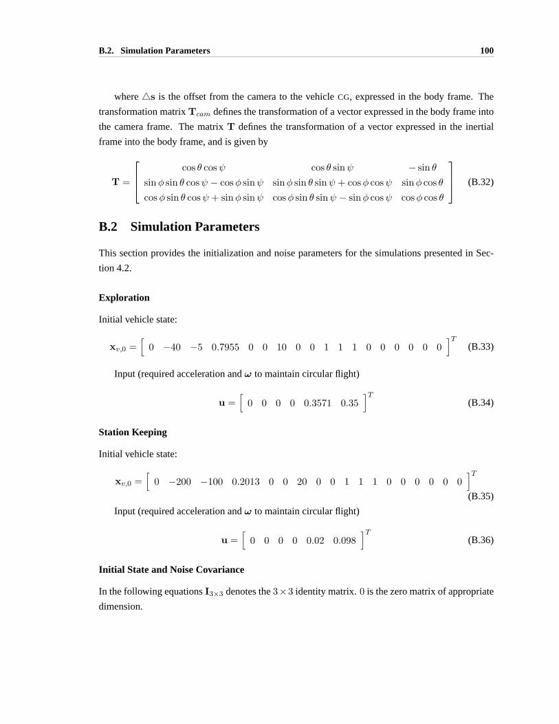
B.2. Simulation Parameters 100
where4s is the offset from the camera to the vehicleCG, expressed in the body frame. The
transformation matrixTcam defines the transformation of a vector expressed in the body frame into
the camera frame. The matrixT defines the transformation of a vector expressed in the inertial
frame into the body frame, and is given by
T =
cos θ cosψ cos θ sinψ − sin θsinφ sin θ cosψ − cosφ sinψ sinφ sin θ sinψ + cosφ cosψ sinφ cos θcosφ sin θ cosψ + sinφ sinψ cosφ sin θ sinψ − sinφ cosψ cosφ cos θ
(B.32)
B.2 Simulation Parameters
This section provides the initialization and noise parameters for the simulations presented in Sec-
tion 4.2.
Exploration
Initial vehicle state:
xv,0 =[
0 −40 −5 0.7955 0 0 10 0 0 1 1 1 0 0 0 0 0 0]T
(B.33)
Input (required acceleration andω to maintain circular flight)
u =[
0 0 0 0 0.3571 0.35]T
(B.34)
Station Keeping
Initial vehicle state:
xv,0 =[
0 −200 −100 0.2013 0 0 20 0 0 1 1 1 0 0 0 0 0 0]T(B.35)
Input (required acceleration andω to maintain circular flight)
u =[
0 0 0 0 0.02 0.098]T
(B.36)
Initial State and Noise Covariance
In the following equationsI3×3 denotes the3×3 identity matrix.0 is the zero matrix of appropriate
dimension.

B.2. Simulation Parameters 101
Initial state covariance:
P0 =
0.012I3×3 0 0 0 0 00 0.0012I3×3 0 0 0 00 0 0.012I3×3 0 0 00 0 0 0.012I3×3 0 00 0 0 0 0.0252I3×3 00 0 0 0 0 0.0012I3×3
(B.37)
IMU bias drift covariance:
Σbiases =
0.0012I3×3 0 00 0.0012I3×3 00 0 0.00012I3×3
(B.38)
IMU measurement noise covariance:
Σimu =
[0.082I3×3 0
0 0.0082I3×3
](B.39)
Vision measurement noise covariance (equivalent to1◦ error in bearing):
Rcam =
[0.01752 0
0 0.01752
](B.40)

Bibliography
[1] Omead Amidi. An Autonomous Vision Guided Helicopter. PhD thesis, Carnegie Mellon
University, Pittsburgh, PA, August 1996.
[2] Tim Bailey. Constrained initialisation for bearing-only SLAM. InIEEE International Confer-
ence on Robotics and Automation (ICRA), Taipei, Taiwan, 2003. IEEE.
[3] J. Biesiadecki, C. Leger, and M. Maimone. Tradeoffs between directed and autonomous
driving on the Mars Exploration Rovers. InInternational Symposium of Robotics Research,
San Francisco, California, October 2005.
[4] John H. Blakelock.Automatic Control of Aircraft and Missiles. Wiley Interscience, New York,
2nd edition, 1991.
[5] M. Bosse, P. Newman, J. Leonard, M. Soika, W. Feiten, and S. Teller. An atlas framework
for scalable mapping. InProceedings of the IEEE International Conference on Robotics and
Automation (ICRA), 2003.
[6] Jean-Yves Bouget. Camera calibration toolbox for matlab. http://www.vision.caltech.edu
/bouguetj/calibdoc/index.html.
[7] Arthur E. Bryson.Control of Spacecraft and Aircraft. Princeton University Press, Princeton,
New Jersey, 1994.
[8] Darius Burschka and Gregory D. Hager. V-GPS(SLAM): Vision based inertial system for
mobile robots. InIEEE International Conference on Robotics and Automation, New Orleans,
LA, April 2004.
[9] Yang Cheng, Mark Maimone, and Larry Matthies. Visual odometry on the Mars Exploration
Rovers. InIEEE Conference on Systems, Man and Cybernetics, The Big Island, Hawaii,
October 2005.
[10] Andrew J. Davison. Real-time simultaneous localisation and mapping with a single camera.
In International Conference on Computer Vision, Nice, France, October 2003.
102
BIBLIOGRAPHY 103
[11] David D. Diel, Paul DeBitetto, and Seth Teller. Epipolar constraints for vision-aided inertial
navigation. InIEEE Workshop on Motion and Video Computing. IEEE, 2005.
[12] Gamini Dissanayake, Stefan B. Williams, Hugh Durrant-Whyte, and Tim Bailey. Map man-
agement for efficient simultaneous localization and mapping (SLAM). InAutonomous Robots
12, pages 267–286, 2002.
[13] Bernard Etkin and Lloyd Duff Reid.Dynamics of Flight: Stability and Control. John Wiley
& Sons, New York, 3rd edition, 1996.
[14] R. Eustice, H. Singh, J. Leonard, M. Walter, and R. Ballard. Visually navigating the RMS
Titanic with SLAM information filters. InProceedings of Robotics: Science and Systems
(RSS), Cambridge, MA, USA, June 2005.
[15] Trevor Fitzgibbons and Eduardo Nebot. Bearing only SLAM using colour-based feature track-
ing. In 2002 Australasian Conference on Robotics and Automation, Auckland, New Zealand,
2002.
[16] Eric Foxlin and Leonid Naimark. Vis-tracker: A wearable vision-inertial self-tracker. InIEEE
VR2003, Los Angeles, California USA, March 2003. IEEE, IEEE.
[17] D. Hsu, R. Kindel, J. C. Latombe, and S. Rock. Randomized kinodynamic motion planning
with moving obstacles.International Journal of Robotics Research, 21(3):233–255, March
2002.
[18] Andreas Huster and Steve Rock. Relative position sensing by fusing monocular vision and
inertial rate sensors. In11th International Conference on Advanced Robotics (ICAR), 2003.
[19] Joam Sola i Ortega, Thomas Lemaire, Michel Decy, Simon Lacroix, and Andre Monin. De-
layed vs undelayed landmark initialization for bearing only SLAM. InWorkshop on Sim-
ulateous Localisation and Mapping, International Conference on Robotics and Automation,
Barcelona, Spain, 2005.
[20] Jung Soon Jang.Nonlinear Control Using Discrete Time Dynamic Inversion Under Input
Saturation: Theory and Experiment on the Stanford Dragonfly UAVs. PhD thesis, Stanford
University, Department of Aeronautics and Astronautics, December 2003.
[21] S. J. Julier and J. K. Uhlmann. A new extension of the Kalman filter to nonlinear systems.
In AeroSense: The 11th Symposium on Aerospace/Defence Sensing, Simulation and Controls,
Orlando, Florida, 1997.

BIBLIOGRAPHY 104
[22] Simon Julier and Jeffrey Uhlmann. Reduced sigma point filters for the propagation of means
and covariances through nonlinear transformations. InAmerican Controls Conference, An-
chorage, Alaska, May 2002.
[23] Simon Julier, Jeffrey Uhlmann, and Hugh F. Durrant-Whyte. A new method for the nonlin-
ear transformation of means and covariances in filters and estimators.IEEE Transactions on
Automatic Control, 45(3):477–482, March 2000.
[24] T. Kailath, A. H. Sayed, and B. Hassibi.Linear Estimation. Prentice-Hall, 1st edition, March
2000.
[25] Jong Hyuk Kim and Salah Sukkarieh. Airborne simultaneous localisation and map building.
In IEEE International Conference on Robotics and Automation (ICRA), Taipei, Taiwan, 2003.
IEEE.
[26] Jong Hyuk Kim and Salah Sukkarieh. Recasting SLAM–towards improving efficiency and
platform independency. In11th International Symposium of Robotics Research (ISRR), Siena,
Italy, 2003.
[27] Jonghyuk Kim and Salah Sukkarieh. Autonomous airborne navigation in unknown environ-
ments.IEEE Transactions on Aerospace and Electronic Systems, 40(3):1031–1045, July 2004.
[28] N. M. Kwok and G. Dissanayake. An efficient multiple hypothesis filter for bearing-only
SLAM. In Interational Conference on Intelligent Robots and Systems, Sendai, Japan, 2004.
[29] K. N. Leabourne, S. M. Rock, S. D. Fleischer, and R. L. Burton. Station keeping of an ROV
using vision technology. InOCEANS 97 Conference, volume 1, pages 634–640, Halifax, Nova
Scotia, October 1997. MTS/IEEE.
[30] Yufeng Liu and Sebastian Thrun. Results for outdoor-SLAM using sparse extended informa-
tion filters. In IEEE International Conference on Robotics and Automation (ICRA), Taipei,
Taiwan, 2003. IEEE.
[31] Jorge Lobo and Jorge Dias. Integration of inertial information with vision. In24th Conference
of IEEE Industrial Electronics Society (IECON), pages 1263–1267, Aachen, Germany, 1998.
IEEE.
[32] Richard L. Marks.Experiments in Visual Sensing for Automatic Control of an Underwater Ro-
bot. Ph.d. thesis, Stanford University, Department of Aeronautics and Astronautics, Stanford
CA 94305, June 1995. Also published as SUDAAR 681.

BIBLIOGRAPHY 105
[33] Marci Meingast, Christopher Geyer, and Shankar Sastry. Vision based terrain recovery for
landing unmanned aerial vehicles. InConference on Decision and Control, Bahamas, Decem-
ber 2005. IEEE.
[34] Luis Montesano, Jose Gaspar, Jose Santos-Victor, and Luis Montano. Fusing vision-based
bearing measurements and motion to localize pairs of robots. InInternational Conference on
Robotics and Automation, Barcelona, Spain, 2005.
[35] Jose Neira, Maria Isabel Ribeiro, and Juan Domingo Tardos. Mobile robot localization and
map building using monocular vision. InFifth International Symposium on Intelligent Robotic
Systems, Stockholm, Sweden, 1997.
[36] Jose Neira and Juan D. Tardos. Data association in stochastic mapping using the joint com-
patibility test. IEEE Transactions on Robotics and Automation, 17(6):890–897, December
2001.
[37] Thomas Netter and Nicolas Franceschini. A robotic aircraft that follows terrain using a neuro-
morphic eye. InIEEE/RSJ International Conference on Intelligent Robots and Systems (IROS),
Lausanne, Switzerland, 2002.
[38] Ingemar Nygren.Terrain Navigation for Underwater Vehicles. Ph.d. thesis, Royal Institute of
Technology (KTH, Stockholm, Sweden, 2005.
[39] O-Navi. http://www.o-navi.com.
[40] O-Navi, LLC, PO Box 27213, San Diego CA 92198-1213.Phoenix/AX 6DOF/GPS Sensor
Module Quick Start Guide, rev. x10 edition, April 2004.
[41] L. Pedersen, M. Bualat, D. Lees, D. Smith, and R. Washington. Integrated demonstration of
instrument placement, robust execution and contingency planning. IniSAIRAS, Nara, Japan,
2003.
[42] M. Pollefeys, L. Van Gool, M. Vergauwen, K. Cornelis, F. Verbiest, and J. Tops. 3D capture
of archaeology and architecture with a hand-held camera. InISPRS workshop on Vision Tech-
niques for Digital Architectural and Archaeological Archives, pages 262–267, Ancona, Italy,
July 2003.
[43] Richard J. Prazenica, Adam Watkins, Andrew J. Kurdila, Qi Fa Ke, and Takeo Kanade. Vision-
based Kalman filtering for aircraft state estimation and structure from motion. InAIAA Guid-
ance, Navigation and Control Conference, San Francisco, California, August 2005. American
Institute of Aeronautics and Astronautics.
BIBLIOGRAPHY 106
[44] Alison Proctor and Eric N. Johnson. Vision-only approach and landing. InAIAA Guidance,
Navigation and Control Conference, San Francisco, California, August 2005. American Insti-
tute of Aeronautics and Astronautics.
[45] Kristof Richmond and Stephen Rock. A real-time visual mosaicking and navigation system.
In Unmanned Untethered Submersible Technology, Durham, New Hampshire, August 2005.
AUSI.
[46] Jonathan M. Roberts, Peter I. Corke, and Gregg Buskey. Low-cost flight control system for a
small autonomous helicopter. In2002 Australasian Conference on Robotics and Automation,
Auckland, New Zealand, November 2002. ARAA.
[47] Stergios I. Roumeliotis, Andrew E. Johnson, and James F. Montgomery. Augmenting iner-
tial navigation with image-based motion estimation. InIEEE International Conference on
Robotics and Automation (ICRA), Washington, DC, 2002. IEEE.
[48] Srikanth Saripalli, James F. Montgomery, and Gaurav S. Sukhatme. Vision-based autonomous
landing of an unmanned aerial vehicle. InInternational Conference on Robotics and Automa-
tion, pages 2799–2804, Washington DC, May 2002. IEEE.
[49] Bruno Sinopoli, Mario Micheli, Gianluca Donato, and T. John Koo. Vision based navigation
for an unmanned aerial vehicle. InIEEE International Conference on Robotics and Automa-
tion (ICRA). IEEE, 2001.
[50] R. C. Smith and P. Cheeseman. On the respresentation and estimation of spatial uncertainty.
International Journal of Robotic Research, 4(5), 1986.
[51] S. Thrun and Y. Liu. Multi-robot SLAM with sparse extended information filers. InProceed-
ings of the 11th International Symposium of Robotics Research (ISRR’03), Sienna, Italy, 2003.
Springer.
[52] Sebastian Thrun, Wolfram Burgard, and Dieter Fox. A real-time algorithm for mobile robot
mapping with applications to multi-robot and 3d mapping. InIEEE International Conference
on Robotics and Automation (ICRA), San Francisco, CA, 2000. IEEE.
[53] Sebastian Thrun, Dieter Fox, and Wolfram Burgard.Probabilistic Robotics. MIT Press, Sep-
tember 2005.
[54] R. van der Merwe and E. Wan. The square-root unscented Kalman filter for state and
parameter-estimation. InIEEE International Conference on Acoustics, Speech and Signal
Processing, Salt Lake City, UT, 2001. IEEE.

BIBLIOGRAPHY 107
[55] Rudolph van der Merwe, Eric Wan, and Simon Julier. Sigma point Kalman filters for nonlin-
ear estimation and sensor fusion: Applications to integrated navigation. InAIAA Guidance,
Navigation and Controls Conference, Providence, RI USA, August 2004. American Institute
of Aeronautics and Astronautics.
[56] Thomas P. Webb, Richard J. Prazenica, Andrew J. Kurdila, and Rick Lind. Vision-based
state estimation for uninhabited aerial vehicles. InAIAA Guidance, Navigation and Control
Conference, San Francisco, California, August 2005. American Institute of Aeronautics and
Astronautics.
[57] Stefan B. Williams, Gamini Dissanayake, and Hugh Durrant-Whyte. Field deployment of the
simultaneous localisation and mapping algorithm. In15th IFAC World Congress on Automatic
Control, Barcelona, Spain, June 2002.
[58] Allen D. Wu, Eric N. Johnson, and Alison A. Proctor. Vision-aided inertial navigation for flight
control. InAIAA Guidance, Navigation and Control Conference, San Francisco, California,
August 2005. American Institute of Aeronautics and Astronautics.